PHYSICAL REVIEW ACCELERATORS AND BEAMS 24, 104801 (2021)

Impedance modeling and its applicationto the analysis of the collective effects

A. Blednykh , G. Bassi, and V. SmalukBrookhaven National Laboratory, Upton, New York 11973, USA

R. LindbergArgonne National Laboratory, Argonne, Illinois 60439, USA

(Received 4 May 2021; accepted 13 September 2021; published 12 October 2021)

Impedance modeling for accelerator applications has improved over the years, largely as a result ofadvances in simulation capabilities. While this modeling has been successful in reproducing certainmeasurements, it is still a significant challenge to predict collective effects in real machines. In this paper,we review our approach to impedance modeling and the subsequent simulations of collective effects. Wediscuss the choice of the electrodynamics codes and the required computer power resources, modeling ofthe geometric, and resistive wall impedances, their comparison with analytical approaches, and theirapplication for simulating of the collective effects with tracking and beam-induced heating.

DOI: 10.1103/PhysRevAccelBeams.24.104801

I. INTRODUCTION

In this paper, we would like to share our experience withimpedance calculation, optimization, and its subsequentapplication to the analysis of collective effects. Our work isbased on several years of research and development forlow-emittance storage rings, and this paper attempts tofocus on those topics that we think may be useful forrecently started upgrade projects and for those that maycome in the future.There are several factors that can limit the performance

of a storage ring, potentially preventing it from achievingits designed for beam parameters. One important targetparameter that can become a limiting factor for low-emittance storage rings as well as for colliders is the beamintensity. For example, the single-bunch and the totalaverage current can be limited by collective instabilitiesand/or beam-induced heating. Localized heating can bemost easily avoided at high-average current if the bunchlength σs is much larger than the radius of the vacuumchamber b, σs ≫ b. Many present facilities such as APS[1], NSLS-II [2], SOLEIL [3], DIAMOND [4], MAX-IV[5], etc., do not satisfy this condition, since their vacuumchamber size b ≥ 11 mm while the bunch length σs ≲ b.Many recent upgrade projects, including the ALS-U [6],

APS-U [7], SIRIUS [8], PETRA-IV [9], SLS-2 [10],

ESRF-EBS [11], and DIAMOND-II [12] do not satisfythis condition on the bunch length either. This is true eventhough the vacuum aperture typically decreases to enablethe stronger magnetic fields required for the multiple bendachromat concept [13], because the natural bunch length inthese rings also decreases. We illustrate this in Table I,where we compare the main parameters of various upgradeprojects from the beam-intensity and heat-load point ofview. We see that while some chamber radii may be assmall as 6 mm, and some projects have high-(∼10 mm) andlow-chamber profiles (∼6 mm), the natural bunch length inall cases is typically two to four times smaller than thechamber radius. Unfortunately, such short and intensebunches typically have large Touschek and intrabeamscattering rates that result in a short lifetime and largeremittance, and furthermore can excite large wakefieldsaround the ring which lead to higher instability growth ratesand beam-induced heating. To mitigate these negativeeffects, all upgrade projects are looking for ways to extendthe bunch length beyond its natural value σs0.The usual way to increase the bunch length employs a

higher harmonic cavity to flatten the accelerating rfpotential and stretch the bunch [14–28]. The total systemis not trivial, and some additional effort is required to tunethe rf systems in such a way that they do not disturboperation of the longitudinal and transverse bunch-by-bunch feedback systems. Furthermore, predicting thelongitudinal dynamics then requires full particle trackinganalysis with all systems involved and including the totalwakefield of the ring. Each project may choose theirpreferred technology for the higher harmonic cavity, andtypically bunch lengthening factors of 2–5 are expected.

Published by the American Physical Society under the terms ofthe Creative Commons Attribution 4.0 International license.Further distribution of this work must maintain attribution tothe author(s) and the published article’s title, journal citation,and DOI.

PHYSICAL REVIEW ACCELERATORS AND BEAMS 24, 104801 (2021)Review Article

2469-9888=21=24(10)=104801(22) 104801-1 Published by the American Physical Society

https://orcid.org/0000-0001-9391-1820

https://crossmark.crossref.org/dialog/?doi=10.1103/PhysRevAccelBeams.24.104801&domain=pdf&date_stamp=2021-10-12

https://doi.org/10.1103/PhysRevAccelBeams.24.104801




https://creativecommons.org/licenses/by/4.0/

https://creativecommons.org/licenses/by/4.0/

Stretching the bunch as much as possible will significantlyreduce image-current heat loads on vacuum components,which is particularly important for in-vacuum undulatorsand cryogenic chambers for superconducting insertiondevices (IDs), since the full gap in these chambers canbe as small as 4–6 mm. In addition, bunch lengthening willresult in smaller wakefield-induced heating in sensitivecomponents such as beam position monitors (BPMs),bellows, gate valves, and stripline kickers, and may reducethe engineering requirements for flexible rf linings and gaptolerances.In addition to the considerations of the bunch length,

smaller chamber sizes make the handling of synchrotronradiation a more challenging issue. In particular, protectingsensitive components requires a variety of absorbers(masks) that may be quite close to the electron beam.Hence, their contribution to the total impedance of the ringneeds to be well analyzed and optimized. In a similarmanner, as the chambers become smaller the impedancecost of any small cavities between the flange joints (Fig. 1)and small bumps caused by the welding process (Fig. 2) canbe significantly enhanced. The former of these can beparticularly important even if the impedance per joint is

small, since impedance effects tend to sum such thathundreds or thousands of such contributions may resultin significant effects.This paper is organized as follows: we begin by

introducing the basic definitions of wakefield and imped-ance, after which we review computer cluster consider-ations and requirements for numerical simulations ofimpedance and collective effects, and then discuss thechoice of the electrodynamics software. Next, we proceedto describe how impedance simulations are done andprovide a few examples illustrating how these simulationsmay be cross-checked with the analytical results, howgeometrical variations in components can lead to importantimpedance consequences, and to what extent each compo-nent can be analyzed individually. These examples aremeant to highlight critical components and show how theirimpedance can be considered. Finally, we describe how touse the computed impedance to make predictions regardingstorage ring performance, including both the beam-inducedheating analysis and its application to tracking studies ofcollective effects and instability thresholds.

FIG. 1. Cross-section view of a flange joint with an rf contactspring between them in the trapezoidal groove. See Fig. 19 formore details.

FIG. 2. Internal view of the attached flange to an Al vacuumchamber by welding. The internal stitch weld was cut out on thetop and the bottom of the vacuum chamber, to minimize itscontribution to the total impedance of the ring.

TABLE I. Parameters of multibend achromat storage rings.

Radius Natural bunch length Number of bunches Revolution period Average current Coefficient

b (mm) σs0ðmmÞ M T0ðμsÞ IaveðmAÞ T0I2ave1012=M

APS-U 11 4.2 48=324 3.68 200 3068=455ESRF-EBS 10=6.5 2.9 192=992 2.8 200 583=112ALS-U 10=6.5 3.5 284 0.66 500 581SLS-2 10 2.7 400 0.97 400 388DIAMOND-II 10 3.2 900 1.87 300 187SIRIUS 12 2.4 863 1.73 500 501PETRA-IV 10 3.3 960=80 7.7 100=80 80=615

BLEDNYKH, BASSI, SMALUK, and LINDBERG PHYS. REV. ACCEL. BEAMS 24, 104801 (2021)

104801-2

II. DEFINITIONS

Wakefields quantify the impulse given by a sourceparticle to another test particle. They are useful to describecollective interactions in an accelerator, since these forcesare typically sufficiently weak and/or localized such thatthe relative positions between particles do not significantlychange during their interaction. Under this assumption thechange in test particle energy is given by integrating thelongitudinal electric field Ek over space, and we can definethe longitudinal wakefield Wkðx; y; sÞ via

Δγ ¼ emc2

Z∞

∞dτEkðx; y; s; τÞ

¼ e2

mc2Wkðx; y; sÞ; ð1Þ

where s is c times the relative arrival time betweenthe source and test particle, τ is the distance along thetrajectory, and c, e, and m are the speed of light, theelectron charge, and its mass, respectively. In the ultra-relativistic limit causality insures that the wakefield van-ishes in front of the source, so thatWkðx; y; s < 0Þ ¼ 0 forultrarelativistic point particles.Wakefields can describe direct space-charge forces and

radiation forces resulting from accelerated charges, but herewe focus on wakefields that arise from the electromagneticinteraction of a particle with the chamber wall. Thesewakefields are typically divided into their resistive andgeometric components: the former arise because the cham-ber walls are not perfect conductors, while the latter aregenerated whenever the boundary conditions at the wallschange due to changes in chamber geometry. We willassume that the chamber dimensions are much largerthan the beam transverse extent, over which distancesWkðx; y; sÞ ≈Wkð0; 0; sÞ ¼ WkðsÞ; Following usual prac-tice, in the following we will refer to WkðsÞ as thelongitudinal wakefield.In analogy with Eq. (1), the transverse wakefield is

defined in terms of the transverse impulse via

Δx0 ¼ eγmc2

Z∞

∞dτ ðEðx; y; s; τÞ þ v × Bðx; y; s; τÞÞ

¼ −e2

γmc2W⊥ðx; y; sÞ: ð2Þ

When the particles are near the reference orbit, we canagain Taylor expand the wakefield. In this case, theexpansion depends upon the transverse offset of boththe source particle xs and the test particle xt, and for thehorizontal plane, we write

Wxðx; y; sÞ ≈WMx ðsÞ þ xsWD

x ðsÞ þ xtWQx ðsÞ; ð3Þ

where WMx is the monopole component, WD

x is the dipolewakefield, and WQ

x is the quadrupolar wakefield—similar

expressions apply along y. If the chamber is left-right andtop-bottom symmetric WM⊥ ¼ 0, while WQ

⊥ vanishes inaxially symmetric structures. Furthermore, since WD⊥ is thedominant driver of transverse instabilities, the dipole wake-field is often simply referred to as the transverse wakefield.The total energy loss (or total kick) is obtained by

summing the contributions from all source particles. Forexample, if the beam has Np particles that are Gaussiandistributed with rms length σs, then the energy loss of aparticle located at position s is

Δγ ¼ e2Ne

mc2

Zds0 Wkðs − s0Þ e

−s02=2σ2sffiffiffiffiffiffi2π

pσs

: ð4Þ

Similar expressions apply for the transverse kick. Hence,the point-particle wakefields Wk and W⊥ serve as Greenfunctions for the longitudinal and transverse impulses.Finally, since the force is in the form of the convolution

(4), it is often useful to consider the Fourier transform of thewakefields, namely, the impedance. Indeed, in Fourierspace Eq. (4) can be interpreted as the familiar relationVðωÞ ¼ ZðωÞIðΩÞ, with the impedances

ZkðωÞ ¼1

c

Zds eiωs=cWkðsÞ; ð5Þ

Zx;yðωÞ ¼ic

Zds eiωs=cWx;yðsÞ: ð6Þ

III. ELECTROMAGNETIC SIMULATIONS

The most comprehensive approach to estimate instabilitythresholds for accelerator projects is to carry out computersimulation studies that track particles through the ring inthe presence of all the relevant wakefields (or, equivalently,the impedances). The wakefields are in turn computed fromeach vacuum component that is seen by the beam. Thesevacuum components may have complex three-dimensional(3D) geometries, and part of the design process shouldinclude minimizing the impedance as much as possiblewhile satisfying other design constraints, e.g., space andcost. Hence, some effort should be spent calculating theimpedance and verifying that it satisfies requirements.There are several two-dimensional (2D) and 3D electro-magnetic codes that can compute wakefields and/or imped-ances by simulating the interaction of a charged particlebeam with the vacuum chamber in the time-domain and/orfrequency-domain. These codes include GdfidL [29], CST

Particle Studio [30], HFSS [31], ECHOz1/z2 [32,33], ECHO 3D

[34], URMEL [35], Vorpal [36], ACE3P [37], ABCI [38], andPoisson/Superfish [39].Each code has its advantages and disadvantages, and

everyone must decide for themself which simulation pack-age to use. Some factors that one may consider for code

IMPEDANCE MODELING AND ITS APPLICATION … PHYS. REV. ACCEL. BEAMS 24, 104801 (2021)

104801-3

selection were presented in Refs. [40,41], where the authorsmade a detailed comparison between several time-domaincodes using an example tapered transition structure that iscommon in accelerators. Part of the selection processshould consider its ability to use parallel computingresources, particularly if one plans to calculate the imped-ance of complex geometries in 3D.Regardless of the code chosen, an important part of

wakefield simulation is determining the accuracy andnumerical resolution required for a particular component.Codes typically calculate the wakefield from a Gaussianbunch of rms length σ̄s, so that the numerical mesh needs tobe small enough to resolve both σ̄s and the geometricalfeatures of the chamber under consideration [42].Furthermore, when the wakefield is to be used as apseudo-Green function in tracking simulations that deter-mine how collective effects impacts the dynamics, onetypically needs to properly identify σ̄s. Simulations designedto calculate rf heating and/or evaluate low-frequency modesmay calculate the wakefield using a source current whoselength equals that of the bunch in the storage ring, σ̄s ¼ σs0.On the other hand, one would like the wakefield to suitablyapproximate that of a point chargewhen predicting collectiveinstabilities using tracking simulations. In this case, deter-mining the appropriate σ̄s is less straightforward. The generalrule of thumb for tracking is that the wakefield should becalculated with a source current whose length is ten timessmaller than that of the equilibrium beam, σ̄s ≈ σs0=10. Inour experience, this guideline gives a reasonable estimate ofthe required σ̄s, although we have concluded that the actualrequirements are set by the impedance under consideration.Specifically, we observe in Sec. VII that σ̄s must be smallenough to fully resolve the frequency of the first large,resonancelike feature of the impedance. Unfortunately, thisrequirement is not fully prescriptive in that it does notprecisely define the resonance. Nevertheless, we have foundit helps explain why values of σ̄s between σs0=10 and σs0=15give convergent predictions in particle tracking.As an example of how mesh size (and, hence, simulation

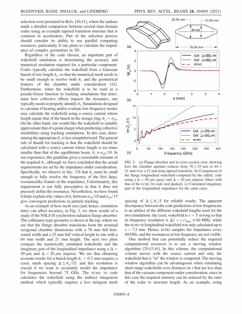
time) can affect accuracy, in Fig. 3, we show results of astudy of the NSLS-II synchrotron radiation flange absorber.The collimator-type geometry is shown at the top, where wesee that the flange absorber transitions from the nominaloctagonal chamber dimensions with a 76 mm full hori-zontal width and a 25 mm full vertical height to one with a64 mm width and 21 mm height. The next two plotscompare the numerically simulated wakefields and theimaginary part of the longitudinal impedance using a Δ ¼50 μm and Δ ¼ 20 μm stepsize. We see that obtainingaccurate results for a bunch length σ̄s ¼ 0.3 mm requires aGdfidL mesh spacing Δ≲ σ̄s=15, and this resolution iscrucial if we want to accurately model the impedancefor frequencies beyond 75 GHz. The ECHO 3D codecalculates the wakefield using the indirect integrationmethod, which typically requires a less stringent mesh

spacing of Δ≲ σ̄s=5 for reliable results. The apparentdiscrepancy between the code predictions at low frequenciesis an artifact of the different wakefield lengths used for thetwo simulations: the GdfidL wakefield is s ¼ 5 m long so thatits frequency resolution is Δf ¼ c=smax ≈ 60 MHz, whilethe ECHO 3D longitudinal wakefieldwas only calculated up tos ¼ 7.5 mm. Hence, ECHO samples the impedance every40 GHz, and the resonances at low frequency are not visible.One method that can potentially reduce the required

computational resources is to use a moving windowalgorithm [29,43,44]. In this scheme, the computationalvolume moves with the source current and only thewakefield that is “in” the window is computed. The movingwindow algorithm can be advantageous when simulatingshort-range wakefields over distances in s that are less thanthat of the vacuum component under consideration, since inthis case the required memory can be reduced by the ratioof the wake to structure length. As an example, using

FIG. 3. (a) Flange absorber and its cross-section view, showinghow the chamber aperture reduces from 76 × 25 mm to 64 ×21 mm over a 12 mm-long tapered transition. (b) Comparison ofthe flange longitudinal wakefield computed by the GdfidL codeusing a Δ ¼ 50 μm (gray) and Δ ¼ 20 μm stepsize (blue) withthat of the ECHO 3D code (red dashed). (c) Calculated imaginarypart of the longitudinal impedance for the same cases.


104801-4

GdfidL to simulate the 150 mm-long NSLS-II rf shieldedbellows with a Δ ¼ 30 μm stepsize and over a wakefieldlength of s ¼ 3 mm requires 218 GB RAM for the“standard” finite-difference time domain algorithm, whilethe moving window needs only 14 GB of RAM. Thismemory difference becomes smaller as the wakefieldlength increases, and whether the moving window providesa memory or computational time advantage depends uponthe code under consideration. We have found that GdfidL’smoving window algorithm (windowwake) is typically notadvantageous for the ≳100 mm wakefield lengths requiredfor most storage ring applications. On the other hand, somecodes (including ECHO) are written to naturally employ amoving window.Finally, a potential shortcoming of finite-difference algo-

rithms is numerical dispersion [42], in which the discretizedmesh modifies the electromagnetic dispersion relation inunphysicalways that depend upon themesh size.Developingalgorithms that are (nearly) dispersion-free over someangular and/or spectral range is not an easy task. It shouldbe noted here that some of the most popular 3D electro-magnetic codes, including GdfidL and CST Particle Studio, arecommercial. Since the GdfidL code has the ability to performparallel computing and has demonstrated reliable results forgeometries with different complexities, both the APS andNSLS-II have used this code as the main tool for thewakefield simulations since the early 2000s.Numerically calculating wakefields and impedances in

complex structures can require significant computationalresources. Hence, the needs of wakefield calculations shouldbe added to those of lattice optimization, beam dynamicssimulations, etc., when obtaining the required computationalresources. If this involves building a dedicated cluster, thefirst step is to consider themaximumplanned capacity so thatspace with enough cooling capacity and power supplies canbe reserved. Two basic models to acquiring the desiredhardware can then be considered: the first option is to attemptto purchase the entire cluster at once as was done forsignificant parts of the APS-U project at ANL; The secondoption is to buy a rack with a couple of nodes and a fastswitch, towhich additional nodes are added as funds becomeavailable over the next several years, as was done for theNSLS-II accelerator physics cluster.Ultimately, the number of multicore processors and the

total RAMmemory drives the cluster cost. For this reason, itis often beneficial to install nodes that have differentcomputing capabilities tailored to differing needs. As anexample, simulations of lattice dynamics do not requiresignificant memory or communication between processors,so that increasing the number of multicore processorsstrongly improves the performance. On the other hand,electromagnetic simulations to obtainwakefields and imped-ances require more communication between nodes and aretypically RAM hungry, particularly when one considershigh-resolution wakefields for complex 3D geometries. In

this case, the minimum amount of required RAM memorycan be estimated as minimum 4 GB per core (task), althoughmore can be quite beneficial.

IV. IMPEDANCE MODELING

We believe that the impedance analysis should begin inthe early stages of any accelerator upgrade project, so that itcan help inform the design of vacuum components. Evenwhen the detailed vacuum system is not known, a prelimi-nary impedance lattice and/or budget can be estimatedusing simplified models of key vacuum chamber compo-nents. Such approximate models can identify the majorsources of impedance early in the design phase, so thatparticular attention can be made to the impedance cost asthe design matures.We have found it useful to summarize the relative

resistive and geometric contributions of the developingimpedance model within a single file that lists all imped-ance elements including its material, length, location in thering, internal dimensions, the computed loss factor, lowfrequency ℑðZkÞ=n, and the betatron function-weightedkick factor. In the early stages of ring design, thesequantities can give rough assessments of rf heating andinstability thresholds. For example, the NSLS-II’s initialestimate for the microwave instability [2] applied Oide andYokoya’s formula [45]

Ithresh ≈ 9.4γmc2ν2s

eαcℑðZk=nÞðω0σs0=cÞ3; ð7Þ

where νs is the synchrotron tune and αc is the momentumcompaction. Equation (7) has the same form as Boussard’sextention [46] to the Keil-Schnell formula but with thefactor 9.4 replacing Boussard’s

ffiffiffiffiffiffi2π

p≈ 2.5. Using Eq. (7)

with a ℑðZk=nÞ ¼ 0.4 Ω that was based upon publishedresults at the APS and ESRF, the first estimate for themicrowave instability threshold was 0.6 mA. This turnedout to be about half of the final measured value of 1.2 mA.Once a more detailed design of the vacuum system

develops, however, the loss factor, ℑðZk=nÞ, and kickfactor are insufficient for detailed predictions of collectiveeffects. Nevertheless, these quantities do provide a quickand easy way to gauge the relative impedance cost ofvarious components and can be particularly useful as ametric for how the impedance contribution of any particularcomponent may change as the design matures.We show an example from the summary that has been

developed at NSLS-II in Fig. 4. The main part describes allthe components in the identical long straight sections ofcells 6, 14, 20, and 26. Various abbreviations have beenused in the table for the names of vacuum components andthe resistive wall surfaces, like bellows (BLW) withstainless steel (SS), silver coated (Ag) and GlidCop


104801-5

(GCu) surfaces, and standard vacuum chamber (CHM)with aluminum (Al).The next two sections further discuss the modeling of

such vacuum components, paying particular attention tofirst the resistive wall contribution that comes about fromlosses in the chamber walls, and then to the geometriccontribution that arises from changes in the chamber crosssection. While some electrodynamics codes can includeboth the geometric and resistive effects in their simulations,we have found that it is often simpler to compute these twosources separately. This approach of separating the twoimpedance contributions has been employed by, e.g., theNSLS-II, APS-U [47], ALS-U, and EIC [48] projects.

A. Resistive wall

Vacuum chamber components with finite conductivityinteract with the beam to produce both longitudinal andtransverse forces. In simple chamber geometries, these forcescan be computed analytically, from which longitudinal andtransverse wakefields and/or impedances may be derived.Our typical approach to computing the resistive wall wake-field is to model each individual component as either acircular chamber or as two parallel plates, and then apply theanalytic wakefields/impedances derived by Piwinski [49],Bane and Sands [50], and Yokoya [51]. The circular modelcan be used when the chamber is approximately azimuthallysymmetric, while the parallel plates model applies when theaspect ratio between the horizontal and vertical dimensionsbecomes large. Calculations for rectangular and ellipticalchambers show that the longitudinal resistive force doesn’tvary much between these two extremes, while the transverseforce is largest for round chambers, and smoothly transitionsto the parallel plate limit as the ratio between the twodimensions becomes larger than 2 to 3.

The longitudinal resistive wall force is the same in bothround and flat chambers. The longitudinal wakefield drivenby a Np particles that are Gaussian distributed with rmswidth σ̄s is

Wrwk ðsÞ ¼ remc2Np

2bffiffiffiffiffiffiffiffiffiffiffiffiffiffiffiffiffiffiffiffi2μrZ0σcon

p�� sσ̄s

��3=2

e−s2=4σ̄2s

× fI1=4ðs2=4σ̄2sÞ − I−3=4ðs2=4σ̄2sÞ− sgnðsÞ½I−1=4ðs2=4σ̄2sÞ − I3=4ðs2=4σ̄2sÞ�g; ð8Þ

where re is the classical electron radius, Z0 ≈ 120π Ω is theimpedance of free space, b is the chamber radius or halfheight, σcon is the chamber’s electrical conductivity, and μris its relative permeability.The vertical resistive wall wakefield was derived ana-

lytically for round and flat vacuum chambers by A.Piwinski [49,52]. Bane and Sands [50] demonstrated thatPiwinski’s result is valid for a long Gaussian bunch whoserms width satisfies σs ≫ s0 ¼ ð2b2=Z0σconÞ1=3, a conditionthat is typically well satisfied in storage rings. Under theseconditions, the radial force generated by a beam that isdisplaced from the axis of a round chamber by an amountro is given by [52]

Wrnd⊥ ðsÞ ¼ 2remc2Np

b3ffiffiffiffiffiffiffiffiffiffiffiffiffiffiffiffiffiffiffiffi2μrZ0σcon

p roe−s2=4σ̄2s

ð1 − r2o=b2Þ2�� sσs

��1=2

× ½I−1=4ðs2=4σ̄2sÞ − sgnðsÞI1=4ðs2=4σ̄2sÞ�: ð9Þ

The force diverges as the beam approaches the wall andro → b, while for small displacements the force scaleslinearly with ro and we can approximate it using the dipolarapproximation W⊥ ≈ roð∂W⊥=∂roÞro¼0 ¼ roW⊥;dip.

FIG. 4. A spreadsheet summary of the impedance contributions with relevant lattice parameters. Component differences amongst thevarious sectors are tracked and updated as changes are made. BLW is the bellows and CHM is the standard vacuum chamber.


104801-6

The transverse force for a beam that is displaced in achamber composed of two flat plates was derived inRef. [49]. The expression for an arbitrary offset is similarin form to that of Eq. (9). Here, we just give the dipolarcomponent of the force along the beam axis that is relevantfor small offsets in a chamber of half height h:

Wflat⊥;dip ¼π2reE0Np

6h3ffiffiffiffiffiffiffiffiffiffiffiffiffiffiffiffiffiffiffiffi2μrZ0σcon

p�� sσ̄s

��1=2

e−s2=4σ̄2s

× ½I−1=4ðs2=4σ̄2sÞ − sgnðsÞI1=4ðs2=4σ̄2sÞ�: ð10Þ

Comparing this to the dipole expression for the roundchamber, we see that the dipole wakefield for round andflat chambers with identical minimum gaps, b ¼ h, arerelated by

Wflat⊥;dipðsÞ ¼π2

12Wrnd⊥;dipðsÞ: ð11Þ

The previous considerations apply to conductive metalsbut modern storage rings often applying thin coatings tocertain chambers to improve their performance. For exam-ple, ceramic chambers used for fast kicker chamberstypically have thin layers of metal applied to improve theirimpedance, while a thin coating of nonevaporable getter(NEG) or similar material has been increasingly employedin small aperture chambers to improve their vacuumperformance. We briefly summarize impedance consider-ations for these chambers below.Highly conductive chambers are inappropriate in areas

where magnetic fields vary rapidly with time, because thetransient eddy currents supported by good conductors willshield part of the magnetic field, resulting in delayed anddistorted magnetic waveforms. Nevertheless, such chambersare often coated with a thin conducting layer to preventdamage and vacuum failure from image currents in the beam.For example, there are five ceramic kicker chambers in theNSLS-II storage ring, all of which are coated with Titanium.However, coating ceramics in complex geometries is adifficult task and verifying the coating thickness and uni-formity is technically challenging. Several light sources,including DIAMOND [53], Pohang Light Source [54], andNSLS-II [55] reported overheating of their ceramics cham-bers, which was believed to have been caused from somecombination of poor coating adhesion and lack of coatinguniformity with appropriate thickness. Predicting the imped-ance of even ideal examples of such layered chambers hashad a complicated past. For example, themultilayer approachfirst derived by Piwinski [56] provides an analytic solution tothe problem, but this solution does not apply in the limit ofvery thin coatings, since his power loss formula, Eq. (18) inRef. [56], incorrectly vanishes in the limit that the coatingthickness goes to zero. Hence, to determine the performanceof the thin coatings that are typically required for acceleratorapplications, one must turn to numerical field matching

techniques as is done in, for example, the ImpedanceWake2Dcode [57] developed at CERN.Finally, there is also a long history that has applied field

matching techniques to compute the impedance in a varietyof other multilayered chambers with linear permeabilities(see, e.g., [58]). Relatively simple analytic expressions fortwo-layered chambers that apply to storage ring parametersare available in, e.g., Ref. [59], while more complicatedcases can again be numerically evaluated using theImpedanceWake2D code [57]. The essential physics canbe estimated by comparing the coating thickness to the skindepth

ffiffiffiffiffiffiffiffiffiffiffiffiffiffiffiffiffiffiffiffiffiffiffiffiffiffi2c=jωjσconZ0

pat the frequency of interest: if the

coating is much thicker than the skin depth, the behavior isdominated by the coating material, while in the oppositelimit the fields predominantly see the inner layer. While thephysics is fairly well understood, characterizing the elec-trical parameters of complex, multimaterial coatings can bequite challenging. For example, while recent measurementsof NEG coatings have significantly improved our under-standing of NEG conductivity [60], there are also indica-tions that the impedance may depend upon the coatinguniformity and deposition technique.

B. Geometric impedance

Strong interaction with other physicists, engineers, andtechnicians in the vacuum, diagnostic, and rf groups is keyto successfully integrating impedance considerations invacuum component design. It may take several iterationswith these groups before all requirements are met and thedesign is finalized. As part of this process, the couplingimpedance is calculated for each individual vacuum com-ponent assuming that there is no cross talk between theneighbor components. In this case, the total wakefield/impedance for the ring is a sum of the individual con-tributions. Here, we describe several examples of wakefieldand impedance analysis for individual components. Webegin with two preliminary examples where analytic resultsare used to verify the code predictions, then continue bydescribing how variations in geometry can affect thegenerated wakefields, and finally conclude by showingtwo contrasting examples when interference/cross talk canbe an issue with when it is not.

1. Verifying code predictions with theory

There are many analytic impedance results for idealizedgeometries that can be used to both estimate the impedanceand to cross-check numerical simulations of various com-ponents. These results are typically restricted to either highor low frequencies, and may be summarized in terms of theloss factor kkðσsÞ or the kick factor k⊥ðσsÞ [61–64]. In thissection, we illustrate the utility of such analytic expressionsusing two examples: the first is a simple step collimator,while the second is for a stripline kicker used in theNSLS-II.


104801-7

One test structure that we have found may be useful tonumerically verify an electromagnetic code is that of anaxially symmetric step collimator. Furthermore, this simplestructure can also give a reasonable first estimate to thewakefields resulting from particle collimators or scrapersthat are used in a real machine. For a cylindrical pipe thatmakes a sudden transition from its nominal radius d to asmaller radius b and then back again, the analyticalexpression for the high-frequency impedance derived byKheifets [58] is

Zstepk ðk ≫ 1=bÞ ¼ ðZ0=πÞ lnðd=bÞ; ð12Þ

assuming that kb < γ. Later, Stupakov, Bane, andZagorodnov showed [65] that the high-frequency limitwhere Eq. (12) applies corresponds to the optical regime, inwhich the field propagation can be approximated alongstraight lines in analogy with ray optics.Figure 5 shows the real and imaginary parts of the

impedance calculated by GdfidL for a step collimator withb ¼ 5 mm and d ¼ 25 mm. The longitudinal wakefield wasdetermined using a 0.3 mm bunch length, and we find thatthe impedance is approximately equal to its theoretical valueZstepk ¼ 193 Ω for frequencies f > 50 GHz ≈ 5c=2πb.Our next example of code verification uses a more

realistic geometry, namely, a stripline kicker that has twoelectrodes spanning 90° each; this geometry was analyzedin more detail in Ref. [66]. While the impedance over thefull frequency range must be numerically calculated, at low

frequencies we can compare numerical predictions totheory. Following Lambertson’s formalism [67], the stri-pline longitudinal beam impedance at low frequency is

ZkðkÞ ¼ g2kZch;k½sin2ðkLÞ − i sinðkLÞ cosðkLÞ�; ð13Þ

where gk is the longitudinal geometric factor, Zch;k is thelongitudinal characteristic impedance, k is the wave num-ber, and L is the electrode length. The geometric factor canbe estimated using the Ng approximation [68]

gk ¼ ϕ=π; ð14Þ

while Zch;k can be approximated by

Zch;k ¼ Zcxl=ffiffiffiffiffigk

p ¼ Z0

2π

lnðd=bÞffiffiffiffiffigkp ; ð15Þ

where b is the radius up to the electrode edge while d is thevacuum chamber radius. Using the data from Ref. [69], theangle ϕ ¼ 90° implies that the longitudinal geometricfactor is gk ¼ 1=2, while b ¼ 27.2 mm, d ¼ 39.6 mm,and L ¼ 310 mm gives a characteristic impedanceZch;k ¼ 31.87 Ω. It should be noted that the gk computedusing this simple approximation is somewhat less than thegk ¼ 0.77 obtained numerically in Ref. [66] using thePoisson code.We use the more accurate result to evaluate the product

g2kZch;k ¼ 18.4 Ω for Eq. (13), and compare the theoreti-cally computed longitudinal impedance to that obtainednumerically for the stripline kicker in Fig. 6. The real 3Dstripline structure has been numerically computed by theGdfidL code (Fig. 6, blue traces), while the red traces are thedata obtained using the analytical approach of Eqs. (13),(14), and (15). We see that the analytic formula provides avery good prediction at low frequencies, and the differencebetween it and the simulation results increase as fincreases. The theory become qualitatively incorrect whenf ≳ 3 GHz, in which case the frequency is larger than thecutoff frequency of the first fundamental longitudinal E01-mode and Eq. (13) no longer applies.

2. Effects of tolerance and variations in geometry

Wakefield analysis typically starts with idealized ver-sion of components and then is refined to the point ofsimulatingwakefields directly fromComputer AidedDesign(CAD)-rendered drawings. Nevertheless, installed compo-nents may be somewhat different from the designs due tomanufacturing tolerances or installation precision, and mayeven differ in unexpectedways.Here, we illustrate how theseissuesmay affect the impedance using two examples: the firstuses an example from the APS to show how small geometrychanges can have a big impact on the impedance if it is closeto the particle beam. The second illustrates how installation

FIG. 5. Real (top) and imaginary (bottom) part of the longi-tudinal impedance for the step transition.


104801-8

variations may affect wakefield performance. In an idealworld, one would identify and analyze all such effects andtake them into account during design, but this is, in ouropinion, unrealistic. Nevertheless, we think that these exam-ples show that one should be particularly careful in the designof components that are close to the beam and expected togenerate fairly large wakefields, and furthermore that sometolerance studies of critical components should be done toanticipate how installation variations may affect rf heating.Transitions to and from narrow gap IDs can be a

significant source of transverse impedance at storage ringlight sources. At the APS, the vertical gap of the vacuumchamber reduces from its nominal 42 mm to a minimumbetween 5 and 8 mm depending upon the ID, such thatapproximately one-third of the vertical impedance is due toID transitions themselves, while nearly another third is dueto the resistive wall in the narrow gap ID chamber. Toreduce the impedance of the transitions, Y.-C. Chaenumerically optimized a two-taper scheme, with the result-ing geometry shown in Fig. 7(a). This design reduces theimpedance partly because of its larger slope at largeraperture, and partly by asymmetrically reducing the largewidth, as was subsequently explained by Stupakov [61].The optimized ID transition was installed in the APS

storage ring and its impedance was measured by the localbump method [70,71], with the expectation that themeasured vertical kick factor would be reduced by ∼30.Unfortunately, it was observed that the “optimized” kickfactor was about 20% larger than that of the usualtransition. Additionally, the aperture as measured by the

electron beam was 1 to 2 mm smaller than expected. Forthis reason, the chamber was replaced.After the optimized ID chamber was removed, subsequent

measurements revealed an unusually large weld bead at bothends. The weld bead was located where the transition joinedthe narrow gap ID straight, andmeasured to protrude into thechamber by an average height∼0.8 mm.This discovery bothexplained the measured reduction in the aperture and wouldalso lead to additional wakefields that were not accounted forin the initial analysis. To determine whether the weld beadscould account for our wakefield measurements, we usedGdfidL to compute the kick factor of the new transitionincluding obstacles (weld beads) of varying heights. Theresults are plotted in Fig. 7(b), where we see that smallobstacleswhoseheight is∼0.6 mmeliminate any impedanceadvantage of the optimized transition. Furthermore, weexpect that the measured 0.8 mm weld beads will actuallyincrease impedance. For comparison, Fig. 7(b) also includesthe theory of small obstacles from Refs. [72–74], while weexpect the predicted quadratic increase of the kick factor onheight, the quantitative agreement is somewhat surprisingsince the theory is idealized.The simulation results in Fig. 7(b) are for the transition

alone, but comparisons to the experiment must also includethe contribution due to the resistive wall of the 5 m long IDchamber. We plot the total change in the kick factor as afunction of the obstacle height in Fig. 7(c), with theory inred and the measurement labeled by the blue arrow.Figure 7(c) shows that the best estimate of the measuredweld bead height eliminates nearly all the discrepancybetween the ideal optimal and the measurement, but a smalldifference remains. Regardless, these results show howsignificant imperfections and unintentional obstacles canbe, particularly when they occur at narrow apertures.Indeed, for this reason the transitions to and from theIDs in the APS-U have been designed to be cut directlyfrom the ID straight extrusion, thereby ensuring a smoothsurface at the small gap.The second example is based upon numerical simula-

tions of possible bellows designs for the electron-ioncollider (EIC) project [75]. The EIC will have a high-intensity electron beam of 2.5 A with a ∼7 mm bunchlength [76], and one considered bellows solution adapts thecomb-type bellows that was originally developed in theHigh Energy Accelerator Research Organization (KEK) forhigh-current accelerators [77,78]. We chose to start with thedesign optimized by the Sirius project [79] shown in Fig. 8(a), in which a flexible rf contact spring (circled in red) wasintroduced to eliminate higher order modes below 1 GHzby eliminating the capacitive gap between adjacent fingers.This design was then modified to fit the EIC’s 80 mm by36 mm full-gap elliptical chamber, with the result shown inFig. 8(b).The impedance of the comb-type bellows will depend in

part upon the length L that the fingers overlap and the gap g

FIG. 6. Real (top) and imaginary (bottom) part of the longi-tudinal impedance for two 90° electrode angle. The blue trace isthe GdfidL numerically simulated result. The red trace is theanalytical approximation of Eq. (13).


104801-9

between the finger tip and the bellows body [see Fig. 8(c)],and these dimensions will change as the bellows is com-pressed or decompressed. Since the level of compressionwill vary around the ring depending upon available spaceand tolerances, we performed electromagnetic simulationsto determine how the impedance varies with g and L. Weshow in Figs. 9(a) and (b) that stretching the bellows 4 mmfrom its nominal dimensions of g ¼ 20 and L ¼ 8 mm(orange lines) to g ¼ 24 and L ¼ 4 mm (green lines)significantly changes the real part of the longitudinalimpedance below 20 GHz. The appearance of the promi-nent mode near 13 GHz in the stretched bellows (green)results in nearly three times the loss factor when the bunchlength σs < 6 mm. Hence, the level of rf heating can beexpected to vary by a similar amount as the bellowsgeometry changes.We also compare these two results with a different comb

design that has the gap g reduced to 6 mm. Figure 9(c)shows that loss factor for this design is very similar to thatwith the same finger overlap length L ¼ 8 mm when thebunch length is less than the gap length. For longer bunchlengths σs > g the electromagnetic fields are effectivelyshielded such that they cannot penetrate through the slot.

The variations of the impedance shown here can potentiallybe eliminated by adapting a more conventional bellowsdesign with rf fingers. Such a design can also reduce theimpedance by nearly a factor of two, and therefore looksquite promising from an impedance perspective if a suitablewater-cooling solution can be found.

3. Interference effects between components

The assumption that the wakefields from each compo-nent can be separately calculated applies when the geo-metric changes are small or the components are spaced farapart. These conditions typically apply in the arcs of mostrings, typically fail for a series of rf cavities right next toeach other, and may need to be carefully considered inother cases. Here, we contrast the situation of two tran-sitions close together where interference effects can beimportant with that of a BPM-bellows assembly, wherethey can be safely ignored.The NSLS-II has one straight section populated by two

in-vacuum undulators (IVUs) that are close enough suchthat wakefield interference effects can be observed. Wehave found that this interference can lead to significantimpedance contributions above the cutoff frequency.Unfortunately, detailed simulations of these 6–9 m longstructures is computationally demanding, and in 3D mayexceed what one can reasonably achieve. Here, we willillustrate the interference effect using a simplified 2Dcollimator geometry that can be simulated fairly quicklywith the ECHO code [32].Our simplified model of two back-to-back IVU’s assumes

axial symmetry and is sketched inFig. 10. The basic structureinvolves a tapered transition from the maximum radius ofbmax ¼ 12.5 mm to the minimum radius bmin ¼ 2.5 mmover a distance of LTap ¼ 180 mm. The length at theminimum aperture g ¼ 500 mm is six times shorter thanthe real, 3 m magnet length of each IVU; this was chosen toease the computational requirements but does not have a bigimpact on results. We will compare the impedance predic-tions when the transitions are 500 mm apart as shown in

FIG. 7. (a) Geometry of the optimized transition. (b) Simulated change in the kick factor of the optimized transitions from that of theoriginal. The solid blue line is from the theory of small obstacles. (c) Simulated change in the kick factor of the optimized ID includingthe resistive wall as a function of the weld beam height. The beam-based measurement is indicated by the blue arrow.

FIG. 8. (a) Sirius design of the comb-type bellows. (b) Comb-type bellows as adapted for the EIC project with (c) thedimensions of the finger overlap L and gap g.


104801-10

Fig. 10 with the case wherewe simulate a single transitionedstructure and multiply by two.The results for the computed longitudinal impedance are

presented in Fig. 11, where the red trace uses a singletapered collimator, the cyan trace multiplies the singletapered collimator result by 2, and the dark purple trace isfor two back-to-back tapered collimators. The averageimpedance behavior of the back-to-back collimators isvery close to that of twice the single collimator. Inparticular, the two have essentially identical ℑðZk=nÞ ¼ℑðZkÞ=ðω=ω0Þ ≈ 0.28 mΩ for ω → 0, and both agreereasonably well with Yokoya’s analytic result for an axiallysymmetric taper [80],

ℑðZkÞ=n ¼ ω0Z0

4πcðbmax − bminÞ2

LTap; ð16Þ

Using the NSLS-II’s ω0 ¼ 2π × 378.5 kHz and multiply-ing by two yields a theoretical prediction of ℑðZkÞ=n≈0.265 mΩ.While the general behavior of the impedance is similar,

having two back-to-back collimators creates a cavitylikestructure between them. This in turn results in the appear-ance of many higher order modes above the cutofffrequency of fc ≈ 2.4c=2πbmax ¼ 9.2 GHz for the lowestlongitudinal E01-mode like in a circular waveguide. Theforest of modes above 9 GHz can be clearly seen by thepurple lines of Fig. 11.

Figure 12 compares the transverse impedance for thesame three cases. In this case, the cutoff frequency isdefined by the lowest vertical H11-mode, which hasfc ≈ 1.84c=2πbmax ≈ 7 GHz. While again the back-to-back case has a very different higher order mode structure,at frequencies below 7 GHz its impedance is indistinguish-able from that of a single collimator multiplied by two. Thesimulated Z⊥ðω → 0Þ ≈ 4.2i kΩ=m for two back-to-backcollimators is twice that of a single collimator, andfurthermore agrees reasonably well with Yokoya’s calcu-lation for the low-frequency transverse impedance [80,81]:

Z⊥ðω → 0Þ ¼ iZ0

4π

ðbmax − bminÞ2LTapb2min

≈ 2.7i kΩ=m ð17Þ

for our geometry.

FIG. 9. (a) Real part of the impedance for three different sets of finger dimensions for the comb-type bellows. (b) Real part of theimpedance below 20 GHz. (c) Loss factor as a function of bunch length.

FIG. 10. Two back-to-back axially symmetric collimatorsseparated by a 500 mm distance.

FIG. 11. The real (top) and imaginary (bottom) part of thelongitudinal impedance up to 32 GHz frequency range for theaxially symmetric collimators.


104801-11

The previous example showed that the introduction of acavitylike structure between components can lead to animpedance that is not simply the sum of the two contri-butions. In a similar manner, structures that are closelyspaced and periodic may have important interferenceeffects. Extreme examples of such situations includesequences of rf cavities or specially designed corrugatedstructures. Nevertheless, we have found that the wakefieldinterference effects are negligible for most situations thatarise in storage ring.As an extreme example of a situation where interference

effects are small, we consider the APS-U bellows/BPMassembly that will be discussed further in Sec. V and isshown in Fig. 15. Here, we first separately simulated thegreen, central region to assess the impedance characteristicof the BPM buttons shown in gray. We then eliminated thebuttons from the model, and added the rf contact fingersand compression springs to verify that the fingers providedgood rf shielding and that the small cavity formed by thebellows was acceptable. The resulting wakefields areshown in Fig. 13(a). In Fig. 13(b), we compare thewakefield sum of the two contributions from (a) toWjjðsÞ from the full bellows/BPM assembly, showing thatthe two predictions agree quite well.Figure 13(b) indicates that there are cases where the

interference effects within even a single component aresmall. For the bellows/BPM assembly here the twosolutions with different boundary conditions approximatelysum because each is a small perturbation of the other.

Similarly, we have found that interference effects betweendifferent components can be neglected if each structurerepresents a small perturbation (meaning that its impedanceis small), and furthermore that the structures do not form aperiodic array with strong resonantlike effects. Hence, theusual procedure to individually analyze components istypically valid.

V. DATA POST-PROCESSING

Electromagnetic codes typically output the wakefield asa function of distance s behind the peak of a Gaussianelectron bunch. Once this has been computed for variouscomponents, the data can be analyzed and processed forsubsequent simulations. This analysis can be done with anumber of tools including MATLAB, Mathematica, orPython scripts, and usually includes plots of the longi-tudinal and transverse wakefields Wk;⊥ðsÞ, the real andimaginary parts of the associated impedances Zk;⊥ðkÞ,and several other processed quantities. For example, thewakefield for the circulating bunch length σs0 can be found

FIG. 12. The real (top) and imaginary (bottom) part of thetransverse impedance up to 300 GHz frequency range for theaxially symmetric collimators. ImZ⊥ðω → 0Þ ¼ 2.1 kΩ=m percollimator.

FIG. 13. (a) Wakefields from simulations that separatelyfocused on the APS-U bellows and BPM buttons shown inFig. 15. (b) Comparison of the sum between the two contributionsfrom (a) to that of the entire structure.


104801-12

by the following convolution with the pseudo-Green’sfunction:

Wðs; σs0Þ ¼Z

ds0 W̄ðs − s0; σ̄sÞexp

h− ðs−s0Þ2

2ðσ2s0−σ̄2sÞi

ffiffiffiffiffiffiffiffiffiffiffiffiffiffiffiffiffiffiffiffiffiffiffiffiffi2πðσ2s0 − σ̄2sÞ

p : ð18Þ

Figure 14 plots the wakefields computed for the NSLS-IIflange absorber presented in Fig. 3. The dashed dark-cyantrace is the pseudo-Green’s function computed for a σ̄s ∼0.3 mm bunch length and convolved with a 3 mmGaussianbunch. The resulting wakefield agrees perfectly with thepink trace, which is the simulated wakefield from a 3 mmbunch with a stepsize 100 μm.For the beam-induced heating and coupled bunch insta-

bility analysis, the wakefield can be computed using a testbunch whose length equals that circulating in the ring. Inthis case, WkðsÞ can be computed with an increasedstepsize (Δ ∼ 100 μm), which allows for wakefields com-puted over a much longer distance s. Since these long-rangewakefields result in high-resolution impedances, they canbe used to compute electrodynamics parameters such as theshunt impedance ðRshÞ and the quality factor (Q) that arerequired for coupled-bunch instability analysis. In addition,the loss factor and the kick factors that are used for beam-induced heating and for the transverse instability thresholdestimations can also be computed from wakefields obtainedfrom the natural bunch length. We will discuss the lossfactor further in Sec. VI.As an example, we now discuss how such analysis was

applied to the APS-U bellows/BPM assembly shown at thetop of Fig. 15. For this geometry, the radius of the standardvacuum chamber aperture is 11 mm, the BPM buttondiameter is 8 mm, and the downstream and upstream rfcontact fingers are compressed against the central BPMbodypipe that is green in Fig. 15. The simulated real part of theimpedance ℜZkðfÞ is shown in the middle plot. Theimpedance is derived from the longitudinal wakefield of a5mmbunch length usingZkðkÞ ¼ FT½WkðzÞ�=FT½−cQðzÞ�,

where, e.g., FT½QðzÞ� is the Fourier transform of the chargeprofile. The first resonance is observed at ≈11 GHz, whichcould result in significant heating if the bunch length was5 mm (spectrum in red). The APS-U, however, plans tolengthen the bunch to 30 mm to increase lifetime, and weshow that even a 12 mm bunch has a small spectral overlapwith the impedance, and correspondingly small heating. Thisdependence is then summarized at the bottom of Fig. 15,where we plot the loss factor as a function of bunch length.Once the wakefields for each individual component have

been calculated, separate scripts can be used to combine

FIG. 14. Wakefield comparison for the NSLS-II flangeabsorber. The pink trace is the longitudinal wakefield simulateddirectly for a 3 mm bunch length. The dashed dark-cyan trace is apseudo-Green’s function computed for a σ̄s ∼ 0.3 mm bunchlength and then convolved with a 3 mm Gaussian bunch, whichagrees with the direct calculation.

FIG. 15. Top: internal view of the APS-U Bellows/BPMassembly. Middle: plot of the real part of the longitudinalimpedance (blue trace), the Gaussian spectrum for the 5 mmbunch length used to computeWk (red), and the spectrum from a12 mm bunch (purple). Bottom: The loss factor vs the bunchlength for the APS-U bellows/BPM assembly.


104801-13

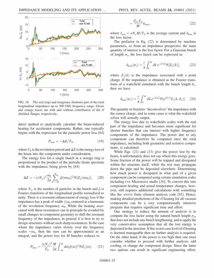
them into a total wakefield that can be used for furthertracking simulations of collective effects. Figure 16 showsall the geometric contributions to the longitudinal wake-field of the NSLS-II [82], which are summed into the totalwakefield plotted in Fig. 17. The first largest sourcescontributing to the longitudinal wakefields are the 739 rfshielded flanges, more than 100 flange absorbers, and ninesmall gap IVUs. Finally, the Fourier transform of the total,ring-averaged wakefield yields the total impedance shownin Fig. 18. Here, we also show how different the predictedimpedance can be if one misses an important component.While the impedance of any single rf-shield flange isrelatively small, the large number of such flanges leads to acritical contribution to the total impedance.The simulation and modeling techniques described here

that compute wakefields and their effects on the beamtypically agree quite well with experiments measuringsingle components. Nevertheless, the predictions madefor an entire facility are often less accurate. Many groups,including SOLEIL, RHIC, Super-KEKB, DIAMOND, andthe NSLS-II have observed discrepancies by a factor of 2 ormore between numerical predictions and experimentalmeasurements in terms of instability thresholds and othercollective effects [83]. There has been much discussion totry to understand why predictions based upon the entireimpedance model often underestimate collective effects.One possible explanation is that the interference effectsdescribed earlier play an important role; another is that theimpedance model has either neglected relevant sources ofimpedance, or simulated idealized models that differ

somewhat from the installed components. Adding up evensmall differences over an entire ring may lead to quitedifferent predictions. Better understanding of the source(s)of the observed discrepancies would be a significantachievement, since it will help improve predictions forfuture upgrade projects and reduce the risk that ringperformance will be unexpectedly limited by collectiveeffects.

VI. BEAM-INDUCED HEATING

The beam-induced heating is of significant concern atmany high-current accelerator facilities. Localized overheat-ing of vacuum components can limit both the single-bunchcurrent and the total average current during the commission-ing phase and regular beam operation. To avoid the disasterof vacuum component deformation, damage and/or failuredue to the image-current heating, temperature transferanalysis should be performed for sensitive vacuum compo-nents before their installation into the ring. While equationsfor purely resistive heating are available, there is at present no

FIG. 16. The NSLS-II longitudinal short-range wakefieldscalculated for a 0.3 mm bunch length for each individualcomponent.

FIG. 17. The total longitudinal wakefield of the NSLS-IIstorage ring (blue trace) as a sum of the resistive wall contribution(green trace) calculated analytically and the geometric wakefields(orange trace).


104801-14

direct method to analytically calculate the beam-inducedheating for accelerator components. Rather, one typicallybegins with the expression for the parasitic power loss [84]

Ploss ¼ −ΔE=T0; ð19Þ

whereT0 is the revolution period andΔE is the energy loss ofthe beam into the component under consideration.The energy loss for a single bunch in a storage ring is

proportional to the product of the periodic beam spectrumwith the impedance, being given by [84]

ΔE ¼ −ðeNpÞ2ω0

2π

X∞n¼−∞

jρ̃ðnω0Þj2ℜ½Zkðnω0Þ�; ð20Þ

where Np is the number of particles in the bunch and ρ̃ isFourier transform of the longitudinal profile normalized tounity. There is a resonant enhancement of energy loss if theimpedance has a peak of width ≲ω0 centered at a harmonicof the revolution frequency ω0. While the heating asso-ciated with these resonances can in principle be avoided bysmall changes in component geometry to shift the resonantfrequency of the impedance, in general it is best to try todesign structures without such sharp resonances. In the casewhere the impedance varies slowly over the frequencyscales ∼ω0, then the sum can be approximated as anintegral, and the power loss for M bunches reduces to

Ploss ¼ðeNeÞ2T0

M2π

Z∞

−∞dωjρ̃ðωÞj2ℜZkðωÞ; ð21Þ

¼ I2aveT0

Mkloss; ð22Þ

where Iave ¼ eNeM=T0 is the average current and kloss isthe loss factor.The prefactor in Eq. (22) is determined by machine

parameters, so from an impedance prespective the mainquantity of interest is the loss factor. For a Gaussian bunchof length σs, the loss factor can be expressed as

klossðσsÞ ¼cπ

Z∞

0

dk e−k2σ2sℜ½ZkðkÞ�; ð23Þ

where ZkðkÞ is the impedance associated with a pointcharge. If the impedance is obtained as the Fourier trans-form of a wakefield simulated with the bunch length σ̄s,then we have

klossðσsÞ ¼cπ

Z∞

0

dk e−k2σ2sℜ½eσ̄2s=2Zkðk; σ̄sÞ�: ð24Þ

The quantity in brackets “deconvolves” the impedance withthe source charge, and in some cases is what the wakefieldsolver will actually output.The energy loss due to wakefields scales with the real

part of the impedance and becomes more significant forshorter bunches that can interact with higher frequencycomponents of the impedance. The power due to anycomponent can therefore be computed once the totalimpedance, including both geometric and resistive compo-nents, is calculated.While Eqs. (22) and (23) give the power lost by the

beam, it unfortunately does not say where this energy goes.Some fraction of the power will be trapped and dissipatedwithin the structure itself, while the rest may propagatedown the pipe and be deposited elsewhere. Determininghow much power is dissipated in what part of a givencomponent can be computed using certain simulation codesincluding CST Microwave studio [30]. To convert this intocomponent heating and actual temperature changes, how-ever, still requires additional calculations with somethinglike the ANSYS finite element analysis code [85]. Hence,making detailed predictions of the rf heating for all vacuumcomponents can be a very computationally intensiveprogram that requires significant time and effort.One strategy to reduce the amount of analysis is to

compute the loss factor using the natural bunch length σs0that does not include any bunch lengthening, and to apply thevery conservative assumption that all the lost energy isdeposited in the structure. If thisworst-case level of rf heatingis deemed manageable then no further analysis is required.On the other hand, if the power is too high then one mustconsider whether to proceed with further analysis, addcooling, or change the component design. Since the lattertwo options can result in significant engineering effort,

FIG. 18. The real (top) and imaginary (bottom) part of the totallongitudinal impedance up to 300 GHz frequency range. Greenand orange traces are with and without contribution of the rfshielded flanges respectively.


104801-15

design complexity, and/or cost, ideally some combination ofanalysis and component design should be used to balanceheatingmarginwith the costs of over-designing components.Even after careful design, it is a good idea to monitor the

temperature of sensitive components during operation. Forexample, the NSLS-II has continually monitored thetemperature of various vacuum components using resis-tance temperature detectors. Temperature monitoring sig-nificantly reduced the risk of unexpected component failureand major vacuum leaks throughout the commissioning andoperating phase as the NSLS-II sought to achieve its targetIave ¼ 500 mA average current.If local heating is observed on an resistance temperature

detectors one can then employ Infrared cameras to moreclearly identify where the temperatures are highest. Weshow a thermal image from an IR camera in Fig. 19(a),which clearly indicates an elevated temperature in theflange joint on the right-hand side of the bellows. Thisjoint was opened during a subsequent maintenance period,and it was found that the spring designed to ensure good rfcontact was not properly installed. Figure 19(b) shows thatthe imprint of the spring contact on the adjoining flangeonly covered part of its surface, indicating poor rf contactbetween the spring and the flange. As shown in Fig. 19(c),this was because the spring was not properly set in itsgroove. The damage to the spring was from synchrotronradiation as it hung into the chamber.

VII. SIMULATING COLLECTIVEEFFECTS WITH TRACKING

It is important to recognize that any attempt to modelcollective effects will only be as good as its ability toproperly identify and model the various sources of imped-ance in the ring [86]. Since any change in the vacuumchamber geometry is a potential source of wakefields,identifying the “important” and/or “relevant” componentsis an art that relies on experience. Previously in the paper,

we have mentioned components that typically must beaccounted for, including BPMs, bellows, ID and rf tran-sitions, flanges, gate valves, rf cavities, photon absorbers,collimators, scrapers, and stripline kickers. Once thecomponents have been identified, electromagnetic solverscan be used to compute the associated wakefield andimpedance of each component as we discussed earlier.Here, we will show how the fidelity of these simulationscan impact tracking predictions of collective effects.Once the impedance elements have been identified and

simulated, they can be used to build an impedance modelfor tracking. The simplest such model lumps all sources ofimpedance into a single “impedance element” that is thenapplied once per turn. The longitudinal impedance withinthis model is determined by summing the impedancecontribution from all components in the ring, Ztot

k ðωÞ ¼Pj Zk;jðωÞ for each component j, while the total transverse

impedance of the ring is found by weighting the individualgeometric contributions by their respective local latticefunctions and summing. More precisely, the total geometricimpedances along x and y are given by

Ztotx ðωÞ ¼ 1

βx

Xelements j

βx;jZx;jðωÞ; ð25Þ

Ztoty ðωÞ ¼ 1

βy

Xelements j

βy;jZy;jðωÞ; ð26Þ

where the lattice functions at element j are denoted by βx;jand βy;j, while βx and βy are the lattice functions at thelocation in the simulated ring where the impedance elementis applied. The influence of collective effects can then becomputed with tracking by inserting the lumped (total)impedance at a single location within a code.The lumped impedance model has proven to be quite

accurate when the collective response is built up over manyturns, as is the case for the longitudinal dynamics and most

FIG. 19. (a) Thermal view of the NSLS-II Bellows with improperly installed the rf contact spring. (b) The SS flange surface has ascratch where the rf spring has good contact, but at least 50% of the area shows little evidence of this contact. (c) Image of the flexible rfspring which was displaced from the trapezoidal grove during installation, and as a result was damaged by synchrotron radiation.


104801-16

transverse instabilities. On the other hand, it is not alwayssufficient to simulate nonequilibrium effects that mightoccur during the transients of particle injection or right aftera kicker has fired [87]. Nevertheless, these cases cantypically be treated using similar techniques if one dividesthe impedance into multiple impedance elements that arethen distributed around the ring.The particle tracking itself can use several models,

ranging from linear maps that include synchrotron emissionto full element-by-element tracking. The former are suffi-cient to model longitudinal collective effects, while addingchromatic variations and lowest-order nonlinearities istypically sufficient to predict transverse stability at equi-librium. Again, predicting transient effects when the beamis potentially far from the nominal orbit presents the mostdemanding simulations, often requiring high-order maps orfull element-by-element tracking.Having outlined the basic methodology, we would like to

discuss some specific details that are important to considerto obtain reliable predictions. We will illustrate these pointswith the impedance model developed for the APS-U. Thefirst thing to recognize is that the most important part of anyimpedance model is identifying all the relevant impedancecontributions. While perhaps obvious, it bears repeatingsince accounting for all of the necessary components isperhaps the least systematic step in the process. Weillustrate this in Fig. 20, where we show what happens ifwe were to forget or miss the contributions of the flangegaps, kicker chambers, and the SS chambers. In this case,the ℑðZkÞ=n decreases by about 25%, and the predictedlevel of bunch lengthening due to the impedance decreasesby a similar amount. Interestingly, the observed microwaveinstability threshold is essentially unchanged. We willexplain the reason for this shortly.In addition to identifying all the components, one must

also decide how to use the simulated wakefields in thetracking. This is complicated by the fact that the wakefieldcalculated from a finite difference solver is computed froma (typically Gaussian) charge distribution with finite extent,while the wakefield from an ultrarelativistic particle is

causal in the sense that it only acts on trailing particles.Several methods have been developed to deal with thismismatch. For example, one can deconvolve the impedancewith the source Gaussian, but this is in general numericallyunstable and therefore only works over a limited frequencyrange. Alternatively, one can “reconstruct” the point-chargewakefield as described in Ref. [88]. This can be quite usefulfor short bunches whose length ≲0.1 mm, but is numeri-cally costly for the bunch lengths typically found storagerings. Another method involves fitting the impedance to anumber of broadband resonators [89], but we have foundthis challenging to do in a general fashion since it requiresspecifying the unknown high-frequency behavior.Furthermore, any similar method leads to fine-structuredwakefields (high-frequency impedance components) thatrequire an extremely large number of particles to reliablysimulate.Since we do not expect that the collective behavior will

depend on the behavior of the wakefield/impedance at verysmall length scales/very high frequencies, our approach hasbeen to simply accept the wakefields as simulated. Then, ifour electromagnetic code derived the wakefield using abunch of length σ̄s, the numerical wakefields used intracking are understood to be the point-charge wakefieldthat has been smoothed by a Gaussian filter of frequencywidth c=σ̄s. The only remaining item is to determinethe required length σ̄s, which effectively means findingthe frequency range over which the impedance affects thedynamics.We have found that obtaining consistent predictions

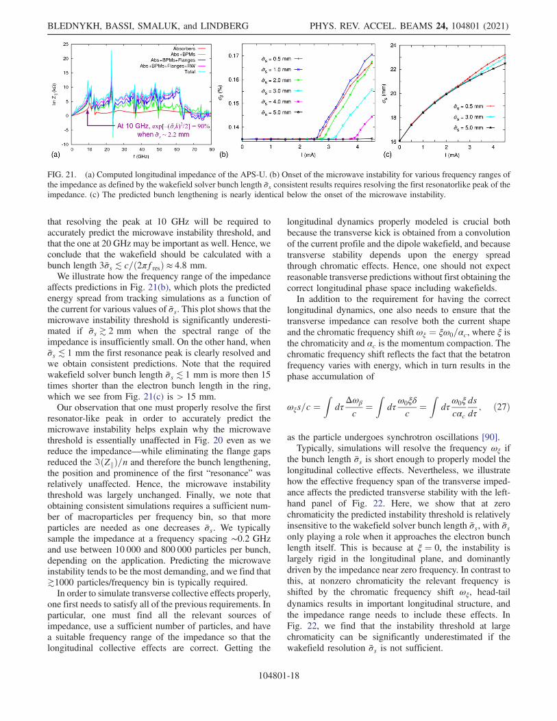
regarding the microwave instability require the bunch lengthσ̄s to be sufficiently short such that it fully resolves the firstlarge resonator-like peak of the impedance. We admit thatthis requirement is only loosely defined, and so we illustrateits use with an example. The APS-U longitudinal impedanceshown in Fig. 21(a) has its first prominent resonance locatednear the cutoff frequency of the 11 mm radius beam pipe.This “resonance” is quite broad and due to several compo-nents including theBPMs and the in-line absorbers,while thesharper resonance near 20GHz is from the BPMs.We expect

FIG. 20. (a) Imaginary longitudinal impedance from the full model (red) and where the flanges, kickers, and SS chambers have beenmissed (blue). (b) shows that the bunch lengthening changes by ∼20%–30%, while (c) indicates that the microwave instability thresholdis approximately unchanged.


104801-17

that resolving the peak at 10 GHz will be required toaccurately predict the microwave instability threshold, andthat the one at 20 GHz may be important as well. Hence, weconclude that the wakefield should be calculated with abunch length 3σ̄s ≲ c=ð2πfresÞ ≈ 4.8 mm.We illustrate how the frequency range of the impedance

affects predictions in Fig. 21(b), which plots the predictedenergy spread from tracking simulations as a function ofthe current for various values of σ̄s. This plot shows that themicrowave instability threshold is significantly underesti-mated if σ̄s ≳ 2 mm when the spectral range of theimpedance is insufficiently small. On the other hand, whenσ̄s ≲ 1 mm the first resonance peak is clearly resolved andwe obtain consistent predictions. Note that the requiredwakefield solver bunch length σ̄s ≲ 1 mm is more then 15times shorter than the electron bunch length in the ring,which we see from Fig. 21(c) is > 15 mm.Our observation that one must properly resolve the first

resonator-like peak in order to accurately predict themicrowave instability helps explain why the microwavethreshold is essentially unaffected in Fig. 20 even as wereduce the impedance—while eliminating the flange gapsreduced the ℑðZkÞ=n and therefore the bunch lengthening,the position and prominence of the first “resonance” wasrelatively unaffected. Hence, the microwave instabilitythreshold was largely unchanged. Finally, we note thatobtaining consistent simulations requires a sufficient num-ber of macroparticles per frequency bin, so that moreparticles are needed as one decreases σ̄s. We typicallysample the impedance at a frequency spacing ∼0.2 GHzand use between 10 000 and 800 000 particles per bunch,depending on the application. Predicting the microwaveinstability tends to be the most demanding, and we find that≳1000 particles/frequency bin is typically required.In order to simulate transverse collective effects properly,

one first needs to satisfy all of the previous requirements. Inparticular, one must find all the relevant sources ofimpedance, use a sufficient number of particles, and havea suitable frequency range of the impedance so that thelongitudinal collective effects are correct. Getting the

longitudinal dynamics properly modeled is crucial bothbecause the transverse kick is obtained from a convolutionof the current profile and the dipole wakefield, and becausetransverse stability depends upon the energy spreadthrough chromatic effects. Hence, one should not expectreasonable transverse predictions without first obtaining thecorrect longitudinal phase space including wakefields.In addition to the requirement for having the correct

longitudinal dynamics, one also needs to ensure that thetransverse impedance can resolve both the current shapeand the chromatic frequency shift ωξ ¼ ξω0=αc, where ξ isthe chromaticity and αc is the momentum compaction. Thechromatic frequency shift reflects the fact that the betatronfrequency varies with energy, which in turn results in thephase accumulation of

ωξs=c ¼Z

dτΔωβ

c¼

Zdτ

ω0ξδ

c¼

Zdτ

ω0ξ

cαc

dsdτ

; ð27Þ

as the particle undergoes synchrotron oscillations [90].Typically, simulations will resolve the frequency ωξ if

the bunch length σ̄s is short enough to properly model thelongitudinal collective effects. Nevertheless, we illustratehow the effective frequency span of the transverse imped-ance affects the predicted transverse stability with the left-hand panel of Fig. 22. Here, we show that at zerochromaticity the predicted instability threshold is relativelyinsensitive to the wakefield solver bunch length σ̄s, with σ̄sonly playing a role when it approaches the electron bunchlength itself. This is because at ξ ¼ 0, the instability islargely rigid in the longitudinal plane, and dominantlydriven by the impedance near zero frequency. In contrast tothis, at nonzero chromaticity the relevant frequency isshifted by the chromatic frequency shift ωξ, head-taildynamics results in important longitudinal structure, andthe impedance range needs to include these effects. InFig. 22, we find that the instability threshold at largechromaticity can be significantly underestimated if thewakefield resolution σ̄s is not sufficient.

FIG. 21. (a) Computed longitudinal impedance of the APS-U. (b) Onset of the microwave instability for various frequency ranges ofthe impedance as defined by the wakefield solver bunch length σ̄s consistent results requires resolving the first resonatorlike peak of theimpedance. (c) The predicted bunch lengthening is nearly identical below the onset of the microwave instability.


104801-18

Finally, the simulations should include both the dipolarwakefield (in which the kick is proportional to the displace-ment of the source particle) and quadrupolar wakefield(where the kick scales with the displacement of the testparticle). Note that this is true even though only the dipolewakefield directly drives the instability, since the quadrupo-lar wakefield results in a tune shift that can indirectly affectstability [91]. We illustrate this in the right-hand panel ofFig. 22, where we have (somewhat artificially) scaled thepredicted APS-U quadrupolar impedance while keeping thedipole impedance fixed. The scaling factor 1 corresponds tothat predicted for the APS-U, while setting the quadrupolarimpedance to zero assumes round chambers everywhere.Since the APS-U has mostly round chambers the limit ofentirely flat chambers leads to increasing the quadrupolarimpedance by a factor of 3.5. Figure 22 shows that thesevariations can lead to significantly different conclusionsregarding transverse stability. Although this example issomewhat contrived, it does illustrate the fact that thequadrupolar impedance can play an important role inpredicting transverse stability.

VIII. CONCLUSIONS

In this paper, we discussed the methods we have used toquantify collective effects in a storage ring. These methodswere used during the design and operating phases of theaccelerator facility, and involved close coordination ofmany groups including those covering accelerator physics,vacuum design, diagnostics, rf, and IDs. A well-estimatedimpedance budget is an important part of predicting theperformance of facilities with intense beams, and suchpredictions should be based on vacuum component designsas installed in the ring. This is particularly important duringthe final stages of component design, manufacture, andinstallation, when seemingly small changes can be intro-duced that may alter the associated impedance.

Once the impedance has been computed, we have shownhow to include collective effects in simulations, payingparticular attention to practical considerations that canaffect the simulations fidelity. We have indicated thataccurate modeling of the longitudinal dynamics is aprerequisite for obtaining reliable transverse calculations,and indicated how we have developed consistent trackingresults. In addition to instability calculations, we havediscussed rf heating as another issue that may limit beamintensity, and discussed methods to predict such heating.We hope that such descriptions will prove useful to othergroups who want to understand collective behavior as partof accelerator and ring design.

ACKNOWLEDGMENTS

This work was supported by Brookhaven ScienceAssociates, LLC under Contract No. DE-SC0012704 withthe U.S. Department of Energy. The work by R. Lindbergwas supported by Department of Energy Contract No. DE-AC02-06CH11357. We would like to thank G. Wang(RHIC) for his help with the ECHO 3D simulation for theNSLS-II flange absorber and K. Shibata (SKEKB) and H.O. Duarte (Sirius) for providing the geometric dimensionsof the comb-type bellows and cross-checking the numeri-cally simulated results. We thank C. Hetzel (EIC) for hisnumerous vacuum system related support. Finally, wewould like to acknowledge M. Borland for help withelegant and a fruitful discussion, L. Emery, Y.-C. Chae,and V. Sajaev for sharing APS data.

[1] P. Den Hartog, J. Gagliano, G. Goeppner, J. Noonan, E.Trakhtenberg, and G. Wiemerslage, Vacuum system of theAPS: Operation experience and status report, in Proceed-

FIG. 22. Dependence of the predicted transverse instability threshold as a function of the transverse impedance extent as characterizedby the wakefield solver bunch length σ̄s. Predicted instability threshold as a function of the strength of the quadrupolar wakefield for theAPS-U, which has most round chambers.


104801-19

ings of the 2001 Particle Accelerator Conference,Chicago, 2001 (JACoW, Geneva, 2001).

[2] Brookhaven National Laboratory, NSLS-II ConceptualDesign Report, 2006, https://www.bnl.gov/nsls2/project/CDR/.

[3] R. Nagaoka, Fast beam-ion instability arising from localoutgassing, in Proceedings of the Topical Workshop onInstabilities, Impedance and Collective Effects 2014(TWIICE 2014) (Synchrotron SOLEIL, 2014).

[4] R. P. Walker, Commissioning and status of the DIAMONDstorage ring, Raja Ramanna Centre for Advanced Tech-nology(RRCAT), Indore, India, TUYMA03, TechnicalReport No. APAC 2007.

[5] MAX-IV Detailed Design Report, available at http://www.maxiv.lu.se/publications.

[6] C. Steier et al., Status of the conceptual design of ALS-U,in Proceedings of IPAC2017, WEPAB104, Copenhagen,Denmark, 2017.

[7] J. Carter, B. Billett, B. Brajuskovic, M. Lale, A. McElderry,J. Noonan, M. O’Neill, K. Wakefield, D. Walters, G.Wiemerslage, and J. Zientek, in MEDSI2018 Proceedingsof the 10th Mechanical Engineering Design of SynchrotronRadiation Equipment and Instrumentation (JACoW,Geneva, 2018), https://doi.org/10.18429/JACoW-MEDSI2018-TUPH04.

[8] R. M. Seraphim, O. R. Bagnato, R. O. Ferraz, H. G. Filho,G. R. Gomes, M. Nardin, R. F. Oliveira, B. M. Ramos,T. M. Rocha, A. R. D. Rodrigues, and M. B. Silva, Vacuumsystem design for the Sirius storage ring, in Proceedings ofIPAC2015, WEPMA003, Richmond, VA, USA, 2015 (JA-CoW, Geneva, 2015).

[9] PETRA-IV Conceptual Design Report, https://bib-pubdb1.desy.de/record/426140/files/DESY-PETRAIV-Conceptual-Design-Report.pdf.

[10] SLS-2 Conceptual Design Report, 2017, https://www.dora.lib4ri.ch/psi/islandora/object/psi%3A34977/datastream/PDF/Streun-2017-SLS-2._Conceptual_design_report-%28published_version%29.pdf.

[11] EBS Storage Ring Technical Report, 2018, https://www.esrf.fr/files/live/sites/www/files/about/upgrade/documentation/Design%20Report-reduced-jan19.pdf.

[12] M. P. Cox, C. W. Burrows, A. G. Day, J. A. Dymoke-Bradshaw, R. K. Grant, N. P. Hammond, X. Liu, A. G.Miller, H. S. Shiers, and N. R. Warner, Conceptual designof the DIAMOND-II vacuum system, in Proceedings ofIPAC2019, TUPMP050, Melbourne, Australia, 2019 (JA-CoW, Geneva, 2019).

[13] D. Einfeld et al., Design of a diffraction limited light source(DIFL), in Proceedings of PAC’95, Dallas, 1995 (JACoW,Geneva, 1995), p. 177.

[14] M. Borland, T. Berenc, R. Lindberg, and A. Xiao, Trackingstudies of a higher-harmonic bunch-lengthening cavityfor the APS Upgrade, in Proceedings of IPAC2015,MOPMA007, Richmond, VA, USA, 2015 (JACoW, Geneva,2015).

[15] R. Lindberg, Theory of coupled-bunch longitudinal insta-bilities in a storage ring for arbitrary RF potentials, Phys.Rev. Accel. Beams 21, 124402 (2018).

[16] R. Warnock and M. Venturini, Equilibrium of an arbitrarybunch train in presence of a passive harmonic cavity:

Solution through coupled Haissinski equations, arXiv:2003.09959.

[17] M. Venturini, Passive higher-harmonic RF cavities withgeneral settings and multibunch instabilities in electronstorage rings, Phys. Rev. Accel. Beams 21, 114404 (2018).

[18] N. Towne and J. Rose, Bunch lengthening harmonicsystem for NSLS-II, in Proceedings of EPAC08, Genoa,Italy, 2008 (JACoW, Geneva, 2008), paper MOPP152.

[19] M. Georgsson, A. Andersson, and M. Eriksson, Landaucavities at MAX-II, Nucl. Instrum. Methods Phys. Res.,Sect. A 416, 465 (1998).

[20] J. M. Byrd, S. De Santis, M. Georgsson, G. Stover, J. D.Fox, and D. Teytelman, Commissioning of a higherharmonic RF system for the Advanced Light Source, Nucl.Instrum. Methods Phys. Res., Sect. A 455, 271 (2000).

[21] M. Pedrozzi et al., SLS operational performance with thirdharmonic superconducting system, in Proceedings of 11thWorkshop on RF superconductivity, Lubeck, Germany.

[22] M. Svandrlik et al., Performance of the 3rd harmonicsuperconducting cavity at ELLETRA, in Proceedings of11thWorkshop on RF superconductivity, Lubeck, Germany.

[23] W. Anders and P. Kuske, HOM damped NC passiveharmonic cavities at BESSY, in Proceedings of 2003Particle Accelerator Conference (JACoW, Geneva,2003), p. 1186.

[24] D. Alesini et al., The DAFNE 3rd harmonic cavity, inProceedings of 2001 Particle Accelerator Conference,Chicago (JACoW, Geneva, 2001), p. 885.

[25] A. Blednykh et al., Harmonic cavity performance forNSLS-II, in Proceedings of 2005 Particle AcceleratorConference, Knoxville, Tennessee, p. 2544 (JACoW,Geneva, 2005).

[26] G. Bassi and Juri Tagger, Longitudinal beam dynamicswith a higher harmonic cavity for bunch lengthening, Int. J.Mod. Phys. A 34, 1942040 (2019).

[27] G. Skripka et al., Commissioning of the harmonic cavitiesin the MAX IV 3 GeV storagering, in Proceedings ofIPAC2016, Busan, Korea, 2016 (JACoW, Geneva, 2016),WEPOW035.

[28] H. Feng et al., Design study on higher harmonic cavity forALS-U, in Proceedings of IPAC2019, Melbourne, Aus-tralia, 2019 (JACoW, Geneva, 2019), WEPRB081.

[29] W. Bruns, http://www.gdfidl.de.[30] CST Particle Studio, http://www.3ds.com.[31] ANSYS HFSS, https://www.ansys.com.[32] I. Zagorodnov and T. Weiland, TE/TM field solver for

particle beam simulations without numerical Cherenkovradiation, Phys. Rev. ST Accel. Beams 8, 042001 (2005).

[33] I. Zagorodnov, Indirect methods for wake potential inte-gration, Phys. Rev. ST Accel. Beams 9, 102002 (2006).

[34] I. Zagorodnov, https://echo4d.de/.[35] U. Laustroer, U van Rienen, and T. Weiland, URMEL and

URMEL-T user guide, DESY, Report No. M-87-03, 1987.[36] VORPAL, https://ice.txcorp.com.[37] ACE3P, https://conf.slac.stanford.edu/cw18/sites/cw18.conf

.slac.stanford.edu/files/broc-ace3p.pdf.[38] Yong Ho Chin, http://abci.kek.jp/abci.htm.[39] SuperFish, https://laacg.lanl.gov/laacg/services/.[40] H. O. C. Duarte, Impedance optimization and wakefield

codes comparison for the Brazilian Light Laboratory, in


104801-20

https://www.bnl.gov/nsls2/project/CDR/




http://www.maxiv.lu.se/publications




https://doi.org/10.18429/JACoW-MEDSI2018-TUPH04




pubdb1.desy.de/record/426140/files/DESY-PETRAIV-Conceptual-Design-Report.pdf





https://www.dora.lib4ri.ch/psi/islandora/object/psi%3A34977/datastream/PDF/Streun-2017-SLS-2._Conceptual_design_report-%28published_version%29.pdf








https://www.esrf.fr/files/live/sites/www/files/about/upgrade/documentation/Design%20Report-reduced-jan19.pdf







https://arXiv.org/abs/2003.09959

https://arXiv.org/abs/2003.09959


https://doi.org/10.1016/S0168-9002(98)00667-6

https://doi.org/10.1016/S0168-9002(98)00667-6

https://doi.org/10.1016/S0168-9002(00)00504-0

https://doi.org/10.1016/S0168-9002(00)00504-0

https://doi.org/10.1142/S0217751X19420405

https://doi.org/10.1142/S0217751X19420405

http://www.gdfidl.de



http://www.3ds.com

http://www.3ds.com

http://www.3ds.com

https://www.ansys.com



https://doi.org/10.1103/PhysRevSTAB.8.042001


https://echo4d.de/

https://echo4d.de/

https://ice.txcorp.com



https://conf.slac.stanford.edu/cw18/sites/cw18.conf.slac.stanford.edu/files/broc-ace3p.pdf









http://abci.kek.jp/abci.htm




https://laacg.lanl.gov/laacg/services/



Proceedings of Topical Workshop on Instabilities, Imped-ance and Collective Effects 2014, TWIICE2014.

[41] V. Smaluk, R. Fielder, A. Blednykh, G. Rehm, and R.Bartolini, Coupling impedance of an in-vacuum undulator:Measurement, simulation, and analytical estimation, Phys.Rev. ST Accel. Beams 17, 074402 (2014).

[42] Handbook of Accelerator Physics and Engineering, editedby A.W. Chao and Maury Tigner (World ScientificPublishing Co., Singapore, 2013), 2nd ed., Chap. 3.

[43] L.-Q. Lee, A. Candel, C. Ng, and K. Ko, A movingwindow technique in parallel finite element time domainelectromagnetic simulation, Technical Report No. SLAC-PUB-14099, 2010.

[44] I. Zagorodnov, Wakefield code ECHO, algorithms and appli-cations, in Proceedings of workshop on Instabilities, Imped-ance and Collective Effects, Abingdon, Oxfordshire, 2016.

[45] K. Oide and K. Yokoya, Longitudinal single-bunch Insta-bility in electron storage ring, KEK Preprint 90-10, 1990.

[46] D. Boussard, Observation of microwave longitudinal in-stabilities in the CPS, CERN, Technical Report no. LabII/RF/INT/75-2, 1975.

[47] R. Lindberg and A. Blednykh, Instability thresholds for theadvanced photon source multi-bend achromat upgrade, inProceedings of the 6th International Particle AcceleratorConference IPAC2015, TUPJE077, Richmond, VA, USA,2015 (JACoW, Geneva, 2015).

[48] A. Blednykh, G. Bassi, M. Blaskiewicz, C. Hetzel, V.Ptitsyn, V. Smalyuk, and F. Willeke, Impedance modelingfor eRHIC, in Proceedings of the 9th InternationalParticle Accelerator Conference IPAC2018, TUPMF027,Vancouver, BC, Canada, 2018 (JACoW, Geneva, 2018).

[49] A. Piwinsky, Wakefields and Ohmic losses in flat vacuumchambers, Deutsches Elektronen-Synchrotron DESY, Tech-nical Report No. DESY-HERA-92-04, 1992.

[50] K. Bane and M. Sands, The short-range resistive wallwakefields, Stanford University, Technical ReportNo. SLAC-PUB-95-7074, 1995.

[51] K. Yokoya, Resistive wall impedance of beam pipes ofgeneral cross section, Part. Accel. 41, 221 (1993).

[52] A. Piwinsky, Wakefields and Ohmic losses in roundvacuum chambers, Deutsches Elektronen-SynchrotronDESY, Technical Report No. DESY-HERA-92-11, 1992.

[53] R. Bartolini (private communication).[54] T. Ha (private communication).[55] A. Blednykh, B. Bacha, G. Bassi, G. Ganetis, C. Hetzel,

H.-C. Hseuh, T. Shaftan, V. Smaluk, and G. Wang, Beam-induced heating of the kicker ceramics chambers atNSLS-II,in Proceedings of NAPAC2016, Chicago, IL, USA, 2016(JACoW, Geneva, 2016).

[56] A. Piwinski, Penetration of the field of a bunched beamthrough a ceramic vacuum chamber with metallic coating,IEEE Trans. Nucl. Sci. 24, 3 (1977).

[57] ImpedanceWake2D, https://twiki.cern.ch/bin/view/ABPComputing/ImpedanceWake2D.

[58] B. W. Zotter and S. A. Kheifets, Impedance and Wakes inHigh-Energy Particle Accelerators (World Scientific,Singapore, 1997).

[59] A. Burov and V. Lebedev, Transverse resistive wallimpedance for multi-layer round chambers, in Proceedingsof EPAC 2002 (JACoW, Geneva, 2002), pp. 1452–1455.

[60] E. Koukovini-Platia, G. Rumolo, and C. Zannini, Electro-magnetic characterization of nonevaporable getterproperties between 220–330 and 500–750 GHz for theCompact Linear Collider damping rings, Phys. Rev. Accel.Beams 20, 011002 (2017).

[61] G. Stupakov, Low frequency impedance of tapered tran-sitions with arbitrary cross sections, Phys. Rev. ST Accel.Beams 10, 094401 (2007).

[62] R. L. Gluckstern, Coupling impedance of a single hole in athick-wall beam pipe, Phys. Rev. A 46, 1106 (1992).

[63] J. J. Bisognano, S. A. Heifets, and B. C. Yunn, Lossparameters for very short bunches, in Proceedings ofEPAC 1988, Rome, Italy, 1988 (JACoW, Geneva, 1988),Vol. 88, p. 708.

[64] G. Stupakov, K. L. F. Bane, and I. Zagorodnov, Impedancescaling for small angle transitions, Phys. Rev. ST Accel.Beams 14, 014402 (2011).

[65] G. Stupakov, K. L. F. Bane, and I. Zagorodnov, Opticalapproximation in the theory of geometric impedance, Phys.Rev. ST Accel. Beams 10, 054401 (2007).

[66] A. Blednykh, B. Bacha, G. Bassi, C. Hetzel, B. Kosciuk, D.Padrazo, T. Shaftan, V. Smaluk, and T. Ha, Beam imped-ance and heating analysis of the diagnostic stripline, Nucl.Instrum. Methods Phys. Res., Sect. A 963, 163729 (2020).

[67] G. R. Lambertson, Dynamic devices-pickups and kickers,in Physics of Accelerators, edited by M. Month and M.Dienes [AIP Conf. Proc. 153, 1413 (1987)].

[68] K.-Y. Ng, Impedances of stripline beam-position monitors,Part. Accel. 23, 93 (1988).

[69] A.Blednykh,G.Bassi, C.Hetzel, B.Kosciuk,D. Padrazo,V.Smaluk, T. Shaftan, and G. Wang, Temperature measure-ments of the NSLS-II vacuum components, in Proceedingsof North American Particle Accelerator Conference, NA-PAC2019, TUPLM36, Lansing, Michigan, 2019 (JACoW,Geneva, 2019).

[70] V. Kiselev and V. Smalyuk, Experimental study of imped-ances and instabilities at the VEPP-4M storage ring, inProceedings of the 1999 DIPAC, Chester, United King-dom, 1999 (JACoW, Geneva, 1999), pp. 1005.

[71] Emery, G. Decker, and J. Galayda, Local bump method formeasurement of transverse impedance of narrow-gap IDchambers in storage rings, in Proceedings of the 2001 PAC,Chicago, USA, 2001 (JACoW, Geneva, 2001), pp. 1823.

[72] S. S. Kurennoy, Beam coupling impedances of obstaclesprotruding into a beam pipe, Phys. Rev. E 55, 3529 (1997).

[73] S. S. Kurennoy and R. L. Gluckstern, Impedances ofazimuthally symmetric irises and cavities with semi-elliptical profile in a beam pipe, Phys. Rev. E 55, 3533(1997).

[74] G. V. Stupakov, Impedance of small obstacles and roughsurfaces, Phys. Rev. ST Accel. Beams 1, 064401 (1998).

[75] Brookhaven National Laboratory, EIC ConceptualDesign Report 2021, https://www.bnl.gov/ec/files/EIC_CDR_Final.pdf.

[76] A. Blednykh, M. Blaskiewicz, D. Gassner, C. Hetzel, B.Lepore, B. Podobedov, V. Ranjbar, M. Sangroula, P. Thie-berger,S.Verdu-Andres,G.Wang, andQ.Wu,Anoverviewofthe collective effects and impedance calculation for theEIC, inProceedingsofIPAC2021,THPAB238,Campinas,SP,Brazil,2021 (JACoW, Geneva, 2021).


104801-21



https://twiki.cern.ch/bin/view/ABPComputing/ImpedanceWake2D








https://doi.org/10.1103/PhysRevA.46.1106





https://doi.org/10.1016/j.nima.2020.163729


https://doi.org/10.1063/1.36380

https://doi.org/10.1103/PhysRevE.55.3529




https://www.bnl.gov/ec/files/EIC_CDR_Final.pdf





[77] Y. Suetsugu, M. Shirai, and K. Shibata, Possibilityof comb-type RF shield structure for high-currentaccelerators, Phys. Rev. ST Accel. Beams 6, 103201(2003).

[78] Y. Suetsugu, K. Kanazawa, N. Ohuchi, K. Shibata, and M.Shirai, Application of comb-type RF shield to bellowschambers and gate valves, in Proceedings of 2005 ParticleAccelerator Conference, Knoxville, Tennessee, 2005 (JA-CoW, Geneva, 2005).

[79] H. O. C. Duarte, R. M. Seraphim, T. M. Rocha, A. R. D.Rodrigues, and P. P. S. Freitas, Design review of bellowsRF-shielding types and new concepts for Sirius, in Pro-ceedings of IPAC2019, Melbourne, Australia, doi: https://doi.org/10.18429/JACoW-IPAC2019-MOPGW001.

[80] K. Yokoya, Impedance of slowly tapered structures,CERN, Geneva, Technical Report No. CERN-SL-90-88-AP, 1990.

[81] G. V. Stupakov, Geometrical wake of a smooth taper, Part.Accel. 56, 83 (1996).

[82] A. Blednykh, G. Bassi, C. Hetzel, B. Kosciuk, andV. Smaluk, NSLS-II longitudinal impedance budget, Nucl.Instrum. Methods Phys. Res., Sect. A 1005, 165349(2021).

[83] V. Smaluk, Impedance computations and beam-basedmeasurements: A problem of discrepancy, Nucl. Instrum.Methods Phys. Res., Sect. A 888, 22 (2018).

[84] A. W. Chao, Physics of Collective Beam Instabilities inHigh Energy Accelerators (Wiley, New York, 1993).

[85] ANSYS Academic Research Mechanical, Release 18.1.[86] A. Blednykh, B. Bacha, G. Bassi, W. Cheng, O. Chubar, A.

Derbenev, R. Lindberg, M. Rakitin, V. Smaluk, M.Zhernenkov, Yu-Chen Karen Chen-Wiegart, and L.Wiegart, New aspects of longitudinal instabilities inelectron storage rings, Sci. Rep. 8, 11918 (2018).

[87] V. Sajaev, R. Lindberg, M. Borland, and S. Shin, Simu-lations and measurements of the impact of collectiveeffects on dynamic aperture, Phys. Rev. Accel. Beams22, 032802 (2019).

[88] B. Podobedov and G. Stupakov, Point-charge wakefieldcalculations from finite length bunch wake potentials,Phys. Rev. ST Accel. Beams 16, 024401 (2013).

[89] R. Nagaoka, Instability studies using evaluated wake fieldsand comparison with observations at SOLEIL, Proc. EPAC2006, 2847 (2006).

[90] B. Zotter and F. Sacherer, Instabilities of relativistic particlebeams in accelerators and storage rings, in Proceedings ofFirst Course of International School of Particle Acceler-ator of the ‘Ettore Majorana’ (JACoW, Geneva, 1976),CERN 77-13, p. 175.

[91] A. Burov and V. Danilov, Suppression of Transverse BunchInstabilities by Asymmetries in the Chamber Geometry,Phys. Rev. Lett. 82, 2286 (1999).


104801-22



https://doi.org/10.18429/JACoW-IPAC2019-MOPGW001

https://doi.org/10.18429/JACoW-IPAC2019-MOPGW001




https://doi.org/10.1016/j.nima.2018.01.047

https://doi.org/10.1016/j.nima.2018.01.047

https://doi.org/10.1038/s41598-018-30306-y




https://doi.org/10.1103/PhysRevLett.82.2286

Date post:	29-Mar-2022
Category:	Documents
Upload:	others
View:	3 times
Download:	0 times

PHYSICAL REVIEW ACCELERATORS AND BEAMS 24, 104801 (2021)

Documents