Constraining temperature distribution inside LIGO test masses fromfrequencies of their vibrational modes

Carl Blair ,1,2,* Yuri Levin,3,4,5,† and Eric Thrane5,‡1Laser Interferometer Gravitational-Wave Observatory (LIGO), Livingston, Louisiana 70754, USA

2OzGrav, University of Western Australia, Crawey, Western Australia 6009, Australia3Center for Theoretical Physics, Department of Physics, Columbia University,

New York, New York 10027, USA4Center for Computational Astrophysics, Flatiron Institute, New York, New York 10010, USA

5OzGrav, School of Physics and Astronomy, Monash University, Clayton, Victoria 3800, Australia

(Received 5 November 2020; accepted 23 December 2020; published 22 January 2021)

Thermal distortion of test masses, as well as thermal drift of their vibrational mode frequencies, present amajor challenge for operation of the Advanced LIGO and Advanced VIRGO interferometers, reducingoptical efficiency, which limits sensitivity and potentially causing instabilities which reduce duty-cycle. Inthis paper, we demonstrate that test-mass vibrational mode frequency data can be used to overcome some ofthese difficulties. First, we derive a general expression for the change in a mode frequency as a function oftemperature distribution inside the test mass. Then we show how the mode frequency dependence ontemperature distribution can be used to identify the wave function of observed vibrational modes. We thenshow how monitoring the frequencies of multiple vibrational modes allows the temperature distributioninside the test mass to be strongly constrained. Finally, we demonstrate using simulations, the potential toimprove the thermal model of the test mass, providing independent and improved estimates of importantparameters such as the coating absorption coefficient and the location of point absorbers.

DOI: 10.1103/PhysRevD.103.022003

I. INTRODUCTION

During Advanced LIGO’s [1] first and second observingruns, about 100 kW of optical laser power circulated inthe Fabry Perot arm cavities of the interferometers [2].During observation run 3, 200–250 kW circulated in thearm cavities [3]. It is planned that this power will increaseto 0.5–1 MW [4]. The heating of mirror surfaces of the testmasses associated with this circulating power presents asignificant technical challenge, since the thermal deforma-tion of mirror leads to the loss of optical efficiency. Opticalefficiency is reduced by increased scattered light lossesfrom nonuniform absorption on the mirrored surfacesthermally deforming the surface and by reduced opticalcoupling between cavities as the beam is altered by thermallensing. The reduced optical efficiency ultimately leadsto a loss of interferometer sensitivity [5]. To address thisproblem, extra heating is applied to the test masses using

specially positioned ring heaters and compensation plates.This is done in such a way that the thermal distortioncaused by the ring heaters and compensation platespartially compensates that caused by the laser beam [6,7].The test masses support a large and complex spectrum of

vibrational modes in the frequency range 5–100 kHz. Thefrequency of these modes depends on the temperaturedistribution inside the test mass. Some of these modes arethe drivers of parametric instability [8,9], the control ofwhich was limited by thermal transients [10,11]. Thereforeit is useful to monitor the three-dimensional temperaturefield inside each test mass for optical efficiency andparametric instability control.In this paper we show that components of this temper-

ature field can be measured in real time by monitoring thefrequencies of multiple vibrational modes of the testmasses. Some effort has already been spent designingand implementing a system that monitors small changes inmode frequencies [12,13]. It was shown that hundreds ofvibrational modes are visible at the interferometer output atquiescent amplitudes.These measurements can by extension allow estimates

of the thermal distortion of the test-mass mirror surfacesand distortion in thermo-optic lens in transmission of thetest mass. Hartmann wave front sensors [14] are currentlyused to monitor wave front distortion in the test masses.

*carl.blair@ligo.org†yl3470@columbia.edu‡eric.thrane@monash.edu

Published by the American Physical Society under the terms ofthe Creative Commons Attribution 4.0 International license.Further distribution of this work must maintain attribution tothe author(s) and the published article’s title, journal citation,and DOI.

PHYSICAL REVIEW D 103, 022003 (2021)

2470-0010=2021=103(2)=022003(13) 022003-1 Published by the American Physical Society

The method proposed here compliments wave front sen-sors, providing independent parameter estimates and infor-mation from the temperature field dimension along theoptic axis.The plan of the paper is as follows. In the next section we

develop the mathematical formalism for computing thechanges in mode frequencies. In Sec. III the formalism istested against a COMSOL [15] eigenfrequency analysis. InSec. IV we show how to use the frequency changes to makeinferences about the temperature distribution inside the testmasses, and we discuss limitations of these inferences dueto symmetries of the test masses. In Sec. V the estimatedtemperature distribution from a realistic scenario is exam-ined, and in Sec. VI a Bayesian method for refining test-mass thermal model parameters is described.

II. GENERAL FORMALISM

A. The preamble: Linearity

The changes in the mode frequencies δωi are linearfunctions of the changes in the temperature inside the testmass, δTðrÞ (here and onwards bold-faced letters denotethree-dimensional vectors). Mathematically this can beexpressed as follows:

δωi ¼Z

ρðrÞfiðrÞδTðrÞd3r; ð2:1Þ

where ρðrÞ is the density, and functions fiðrÞ are formfactors that will be discussed in the next subsection. Itis convenient to introduce an inner product betweenfunctions,

hf; gi≡Z

ρðrÞfðrÞgðrÞd3r; ð2:2Þ

and similarly between vector fields,

ha;bi≡Z

ρðrÞaðrÞ · bðrÞd3r: ð2:3Þ

The factor ρðrÞ ensures that the integral is restricted tothe test-mass volume, and as will be seen below, is usefulfor expressing orthogonality relations between the test-mass mode displacements. Equation (2.1) can be writtensimply as

δωi ¼ hfi; δTi: ð2:4Þ

We show in the next subsection how to compute the formfactors.

B. Computation of the form factors f iðrÞConsider a vector Lagrangian displacement ξðr; tÞ of the

test mass from its position of rest. In the linear approxi-mation, the elastodynamic equations of motion are

ρðrÞ ∂2ξ

∂t2 ¼ L̂ðξÞ; ð2:5Þ

where L̂ is the operator representing the elastic restoringforce and given by

L̂ðξÞm ≡ ∂σmn

∂xn ¼ ∂½cmnklϵkl�∂xn ; ð2:6Þ

where

ϵkl ¼ ðξk;l þ ξl;kÞ=2 ð2:7Þ

is the shear tensor, cmnkl is the elasticity tensor, and

σmn ¼ cmnklϵkl ð2:8Þ

is the elastic stress tensor. Here the Einstein convention ofsumming over the repeating tensorial indices is assumed.A normal mode with angular frequency ωi is characterizedby the wave function ξðiÞðrÞ that satisfies the followingeigenequation:

L̂ðξðiÞÞ ¼ −ω2i ρðrÞξðiÞ: ð2:9Þ

Importantly, the normal modes satisfy orthogonalityrelation,

hξðiÞ; ξðjÞi ¼ hξðiÞ; ξðiÞiδij: ð2:10Þ

Consider now a perturbation δL̂ due to the change intemperature of the test mass,

δL̂ðξÞm ¼ ∂∂xn

�δTðrÞ ∂cmnkl

∂T ϵkl

�: ð2:11Þ

Here we take into account the fact that the elasticitytensor is temperature-dependent. Strictly speaking, thereis another contribution to the change in L̂ that is due tothermal expansion of the test mass. However, the thermalexpansion coefficient LIGO test-mass substrate is verysmall. Numerically, it is about 0.003 × dE=dT, where E isthe Young modulus of the fused silica test-mass substrate.Therefore we safely neglect the thermal expansion effect assubdominant.Consider now the first order perturbation theory for

Eq. (2.9), with the perturbed elasticity operator L̂þ δL̂and perturbed normal-mode wave functions ξðiÞ þ δξðiÞ.This gives

δL̂ðξðiÞÞ þ L̂ðδξðiÞÞ ¼ −ω2i ρðrÞδξðiÞ − 2ωiδωiρðrÞξðiÞ:

ð2:12Þ

By requiring that the perturbed eigenfunction has thesame norm as the unperturbed one, we impose an extraconstraint,

CARL BLAIR, YURI LEVIN, and ERIC THRANE PHYS. REV. D 103, 022003 (2021)

022003-2

hξðiÞ; δξðiÞi ¼ 0: ð2:13Þ

We now multiply Eq. (2.12) by ξðiÞ, and integrate over thevolume. Using the orthogonality relations Eqs (2.10) and(2.13), and the self-adjointness of ½1=ρðrÞ�L̂, we get

�ξðiÞ;

1

ρðrÞ δL̂ðξðiÞÞ

�¼ −2ωiδωihξðiÞ; ξðiÞi: ð2:14Þ

Therefore, the change of the mode’s angular frequency isgiven by

δωi ¼ −1

2ωi

hξðiÞ; ½1=ρðrÞ�δL̂ðξðiÞÞihξðiÞ; ξðiÞi : ð2:15Þ

We are now ready to determine the form factor fiðrÞ. Toachieve this, we write down the numerator of the aboveequation explicitly as an integral over volume,

hξðiÞ; ½1=ρðrÞ�δL̂ðξðiÞÞi ¼Z

ξðiÞm δL̂ðξðiÞÞmd3r

¼Z

ξðiÞm∂∂xn

�δTðrÞ ∂cmnkl

∂T ϵðiÞkl

�d3r

¼ −Z

δTðrÞ ∂cmnkl

∂T ϵðiÞmnϵðiÞkl d

3r:

The last step is obtained by integrating by parts, usingGauss’ theorem, recalling that σmn ¼ δσmn ¼ 0 at the sur-face of the test mass, and using the symmetry of theelasticity tensor with respect to the indices m and n (thelatter insures that the stress tensor is symmetric). From thisexpression, we conclude that the form factor is given by

fiðrÞ ¼1

NiρðrÞ∂cmnklðrÞ

∂T ϵðiÞmnðrÞϵðiÞkl ðrÞ; ð2:16Þ

where the normalization factor is given by

Ni ¼ 2ωi

ZρðrÞjξðiÞðrÞj2d3r ¼ 4Ei

ωi; ð2:17Þ

where Ei is the total energy of the mode. It is worth notingthat

cmnklϵmnϵkl ¼ 2UðrÞ; ð2:18Þ

where UðrÞ is the energy density of elastic deformation.For an isotropic medium such as fused silica glass,

cmnklϵmnϵkl ¼ 2UðrÞ ¼ YðϵllÞ2 þ 2μϵsikϵsik; ð2:19Þ

where Y is the Young modulus, μ is the shear modulus, andϵsik is the incompressible part of the shear,

ϵsik ¼ ϵik −1

3ϵllδik: ð2:20Þ

A simple way of rewriting the form factor in Eq. (2.16), thatmay be handy in the context of using materials engineeringpackages like COMSOL or ANSYS, is as follows:

fiðrÞ ¼ωi

2EiρðrÞ�∂UðiÞðrÞ

∂T�ξðiÞ; ð2:21Þ

where the notation implies that the partial derivative withrespect to temperature is evaluated with the mode displace-ment ξðiÞðrÞ being held constant. This completes ourcomputation of the form factors.

III. NUMERICAL TEST AND A PROPOSAL FORPRACTICAL MODE IDENTIFICATION

To validate the form factor solution of Eq. (2.21) it iscompared to a finite element eigenfrequency analysisperformed with COMSOL [15]. The model used is thatof the Advanced LIGO test mass. Model parameters aregiven in Table I and the model geometry is displayedin Fig. 1,The form factors are calculated based on the strain

distribution UðiÞ and total energy Ei of a COMSOLeigenfrequency analysis of the test mass in the ambient(291 K) temperature thermal state. Form factors andthe total mode displacement are shown in Fig. 15 inAppendix A for a selection of modes.An analytically described change in temperature

distribution is defined for the purpose of this test. Thechange in temperature distribution is defined by Zernikepolynominal Z3

1 across the circular surface of the testmass and a uniform distribution through the depth (z) of thetest mass. Two eigenfrequency analyses are run inCOMSOL, one at an ambient temperature of 291 K andthe second with the additional change in temperaturedistribution to produce a two sets of eigenfrequencies.In conjunction, Eqs. (2.4) and (2.21) are used to calculatethe expected change in eigenfrequency for that same

TABLE I. Parameters for the COMSOL model.

Parameter Value Description

Diameter 340.13 mm DiameterDepth 199.59 mm Depthρ 2203 kg=m3 Density (mass 39564g)Wedge 0.07 deg Optic wedgeE 72.7 GPa Young’s modulusσ 0.164 Poisson ratio∂E∂T 11.5 MPa=K Thermal dependence

of Young’s modulus∂σ∂T 1.55 × 10−5=K Thermal dependence

of Poisson ratio

CONSTRAINING TEMPERATURE DISTRIBUTION INSIDE LIGO … PHYS. REV. D 103, 022003 (2021)

022003-3

temperature distribution. The results in Fig. 2 show verygood agreement between the analytical expression and theCOMSOL simulation.The identification of the mode shape of observed

resonances presents a challenge. Parametric instabilities[8] of vibrational modes with frequencies as high as47.5 kHz have been observed at LIGO [13]. At thisfrequency the mode density is high, resulting in severalcandidate modes that could potentially be causing theinstability. Furthermore, theoretical calculations show

that with increased circulating power there might beinstabilities caused by modes with frequencies as high as90 kHz [16]. (The recent installation of acoustic modedampers [17] makes high frequency instabilities a lot lesslikely.) Knowledge of the mode shape is required to designactive control schemes that apply forces to the test masses[10] or optical feedback [18,19]. Currently modes areidentified by comparing observed resonant frequencieswith those computed using finite element modeling.Confident mode identification is currently limited to17 kHz. At higher frequencies, imprecise knowledge ofthe elasticity parameters of fused silica produce largeenough errors such that confusion between modes is aserious issue. The analytical expression for change of modefrequencies as a function of temperature presented herepresents a new tool for mode identification. This couldwork as follows: 1. a well-controlled thermal transientperturbation is applied to the test mass, and the internaltemperature distribution is computed as a function of timeusing finite element modeling. 2. The transient change inmode frequencies can be calculated as a function of timeusing the formalism presented above or finite elementmodeling. 3. These are compared and matched to themeasured transient frequency changes in the monitoredmodes. By following this procedure, mode identificationscan be confirmed. A simulated example of such a con-firmation is shown in Fig. 3 where three modes (coloredgreen) have been deliberately misidentified by switchingtheir indices. Simulated mode frequencies on the verticalaxis are compared with mode frequencies calculated withthe analytical expression of Eq. (2.1). In this case the

FIG. 2. Comparison between the frequency shift predicted by aCOMSOL eigenfrequency simulation and the frequency shiftpredicted by the analytic expression for 225 eigenmodes influ-enced by an arbitrary thermal disturbance. Excellent agreement isobserved.

FIG. 3. The frequency shift predicted by the analytic expressionfor 225 eigenmodes influenced by 1 W of ring heater powerplotted against a simulated measurement including 0.1 mHz noiseand three modes misidentified (green) compared to the expect-ation (red).

FIG. 1. The geometry used for the COMSOL simulation.

CARL BLAIR, YURI LEVIN, and ERIC THRANE PHYS. REV. D 103, 022003 (2021)

022003-4

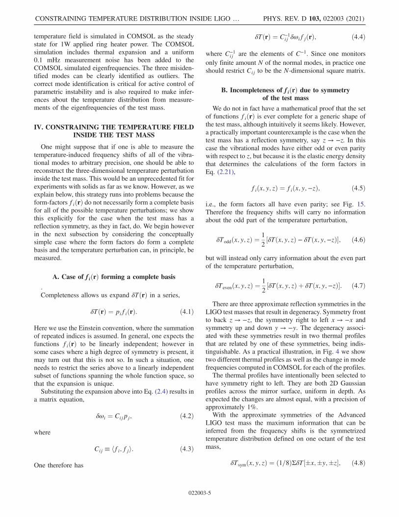
temperature field is simulated in COMSOL as the steadystate for 1W applied ring heater power. The COMSOLsimulation includes thermal expansion and a uniform0.1 mHz measurement noise has been added to theCOMSOL simulated eigenfrequencies. The three misiden-tified modes can be clearly identified as outliers. Thecorrect mode identification is critical for active control ofparametric instability and is also required to make infer-ences about the temperature distribution from measure-ments of the eigenfrequencies of the test mass.

IV. CONSTRAINING THE TEMPERATURE FIELDINSIDE THE TEST MASS

One might suppose that if one is able to measure thetemperature-induced frequency shifts of all of the vibra-tional modes to arbitrary precision, one should be able toreconstruct the three-dimensional temperature perturbationinside the test mass. This would be an unprecedented fit forexperiments with solids as far as we know. However, as weexplain below, this strategy runs into problems because theform-factors fiðrÞ do not necessarily form a complete basisfor all of the possible temperature perturbations; we showthis explicitly for the case when the test mass has areflection symmetry, as they in fact, do. We begin howeverin the next subsection by considering the conceptuallysimple case where the form factors do form a completebasis and the temperature perturbation can, in principle, bemeasured.

A. Case of f iðrÞ forming a complete basis

.Completeness allows us expand δTðrÞ in a series,

δTðrÞ ¼ pifiðrÞ: ð4:1Þ

Here we use the Einstein convention, where the summationof repeated indices is assumed. In general, one expects thefunctions fiðrÞ to be linearly independent; however insome cases where a high degree of symmetry is present, itmay turn out that this is not so. In such a situation, oneneeds to restrict the series above to a linearly independentsubset of functions spanning the whole function space, sothat the expansion is unique.Substituting the expansion above into Eq. (2.4) results in

a matrix equation,

δωi ¼ Cijpj; ð4:2Þ

where

Cij ≡ hfi; fji: ð4:3Þ

One therefore has

δTðrÞ ¼ C−1ij δωifjðrÞ; ð4:4Þ

where C−1ij are the elements of C−1. Since one monitors

only finite amount N of the normal modes, in practice oneshould restrict Cij to be the N-dimensional square matrix.

B. Incompleteness of f iðrÞ due to symmetryof the test mass

We do not in fact have a mathematical proof that the setof functions fiðrÞ is ever complete for a generic shape ofthe test mass, although intuitively it seems likely. However,a practically important counterexample is the case when thetest mass has a reflection symmetry, say z → −z. In thiscase the vibrational modes have either odd or even paritywith respect to z, but because it is the elastic energy densitythat determines the calculations of the form factors inEq. (2.21),

fiðx; y; zÞ ¼ fiðx; y;−zÞ; ð4:5Þ

i.e., the form factors all have even parity; see Fig. 15.Therefore the frequency shifts will carry no informationabout the odd part of the temperature perturbation,

δToddðx; y; zÞ ¼1

2½δTðx; y; zÞ − δTðx; y;−zÞ�; ð4:6Þ

but will instead only carry information about the even partof the temperature perturbation,

δTevenðx; y; zÞ ¼1

2½δTðx; y; zÞ þ δTðx; y;−zÞ�: ð4:7Þ

There are three approximate reflection symmetries in theLIGO test masses that result in degeneracy. Symmetry frontto back z → −z, the symmetry right to left x → −x andsymmetry up and down y → −y. The degeneracy associ-ated with these symmetries result in two thermal profilesthat are related by one of these symmetries, being indis-tinguishable. As a practical illustration, in Fig. 4 we showtwo different thermal profiles as well as the change in modefrequencies computed in COMSOL for each of the profiles.The thermal profiles have intentionally been selected to

have symmetry right to left. They are both 2D Gaussianprofiles across the mirror surface, uniform in depth. Asexpected the changes are almost equal, with a precision ofapproximately 1%.With the approximate symmetries of the Advanced

LIGO test mass the maximum information that can beinferred from the frequency shifts is the symmetrizedtemperature distribution defined on one octant of the testmass,

δTsymðx; y; zÞ ¼ ð1=8ÞΣδT½�x;�y;�z�; ð4:8Þ

CONSTRAINING TEMPERATURE DISTRIBUTION INSIDE LIGO … PHYS. REV. D 103, 022003 (2021)

022003-5

for x, y, z > 0; here Σ denotes the summation over allpossible combination of signs of x, y, z and the origin isassumed to be located at the center of mass of the test mass.There may be a way of breaking some of the degeneracy

by measuring other temperature-sensitive observables suchas the distortion of the mirror’s surface, or the thermallensing of light passing through the test mass, for examplewith the Hartmann sensor. However, we do not considerthese possibilities any further and leave their considerationfor future work.

C. Three-dimensional temperature reconstructionusing singular value decomposition

Suppose now that we are considering properly sym-metrized temperature fields so that fiðrÞ do form acomplete basis. We should still exercise caution usingEq. (4.4) for the temperature field reconstruction. Similaritybetween some form factors fiðrÞ means the C matrix is ill-conditioned (one or more eigenvalues are close to zero),the inversion becomes numerically unstable, leading tounreliable results. A common way of dealing with ill-conditioned matrices is to regularize the matrix by singular-value decomposition (SVD). The conversion matrix isdecomposed into orthogonal matrix U, diagonal matrixC0 and another orthogonal matrix V,

C ¼ UC0V�: ð4:9Þ

We adopt the convention that C0 is defined with valuessorted from largest to smallest along the diagonal. Since Cis real, the Hermitian transpose can be replaced by a regular

transpose V� ¼ VT . By removing eigenmodes associatedwith small eigenvalues, we reduce the dimensionality of C0to N − α by removing the α smallest elements of thecomplete diagonal matrix C0 and the α associate eigen-vectors in U and V. If α is suitably chosen, the resulting“regularized” matrix is numerically invertible. In whatfollows an example of singular value decompositionapplied to simulated eigenfrequency data is demonstrated.The form factors for the first 225 eigenmodes of the test

mass are calculated in COMSOL; each form factor isdefined by the 60000 vertex elements existing in the three-dimensional domain of the test mass. The inner productdefined in Eq. (2.2) is performed to determine the con-version matrix C. Then the singular value decomposition isperformed with Eq. (4.9). The relative numerical value ofthe eigenvalues (diagonal elements of C0) provides ameasure of the additional information that can be recoveredby adding each new element in the SVD. These values areplotted in Fig. 5. From the figure it can be seen that usingmore than 100 SVD elements does not provide a significantincrease in information. It is also interesting to considerthe shape of the largest elements in C0 as these representthe temperature distribution components that will be mosteasily recovered. A selection of C0 eigenfunctions areshown in Appendix B.To demonstrate the usefulness of SVD, we consider a

temperature distribution with rotational symmetry,

T ¼ T0 þ dT ¼ T0 þ ð1=12Þr2; ð4:10Þ

where r is the radial cylindrical coordinate and T0 is aconstant, and compute using Eqs. (2.1) and (2.21) thechanges in the 225 test-mass eigenfreqencies. The temper-ature distribution possesses all the required symmetries andcan thus be recovered by inverting the conversion matrix,with or without using the SVD. The corresponding temper-ature profiles are shown in Figs. 6(a) and 6(b), without anysignificant difference in quality. However if we now

FIG. 4. Comparison of the mode frequency shift betweentwo thermal profiles (inset) that are symmetric left to right.The mode frequencies of the case where the heating is to the leftof the optic axis (vertical axis) are indistinguishable from themode frequencies where the heating is to the right of the opticaxis (horizontal axis).

FIG. 5. Eigenvalues of the SVD matrix C’.

CARL BLAIR, YURI LEVIN, and ERIC THRANE PHYS. REV. D 103, 022003 (2021)

022003-6

assume that the eigenfrequency measurements are notperfect and contain errors, we note a marked differencein the quality of reconstructed temperature fields. As anexample, we add a random frequency error drawn from anormal distribution with width 0.1 mHz to each analyticallycomputed eigenfrequency change and then compute thetemperature fields from this erroneous data set.We observe that the truncated SVD inversion in

Fig. 6(d) produces a significantly better result comparedto the inversion that uses matrix C directly in Fig. 6(c). Thelatter is distorted due to errors in poorly resolvedeignmodes.

The optimal choice for α, the number of excludedeigenvectors, can be estimated for any particular temper-ature distribution, with a particular noise distribution bycomparing the rms error of the temperature estimate,

brms ¼IVjdT − δTjdr: ð4:11Þ

In Fig. 7, the example plot of rms error as a function of thenumber of SVD elements used is shown. This example usesthe same data as Fig. 6. The optimal number of SVDelements is 86. The reconstructed temperature field with 86elements is shown in Fig. 6(d).

V. REALISTIC TEMPERATUREDISTRIBUTIONS

It is useful to reconstruct a temperature field that does notpossesses all the symmetries of the test mass in order to seehow our analysis works in real-world conditions. In thissection we demonstrate that the recovery of symmetrizedtemperature distribution is indeed possible, circumventingthe completeness problem due to test-mass symmetries. Ifthe temperature distribution is not symmetric in the samemanner as the test-mass symmetry the resulting rms error ofthe temperature distribution is large. In Fig. 9 this isdemonstrated. In this case a 100 kW beam on an opticwith a uniform 1 ppm coating absorption is simulatedresulting in a temperature distribution that is relativelyhigher on the high reflectivity surface and relatively cooler

(c)

(a) (b)

(d)

FIG. 6. Profile of estimated temperature distribution inferredfrom changes in eigenfrequecy (a) Inverting Cij directly, (b) SVDinversion using all 225 eigenfrequencies, (c) SVD inversion usingall 225 with 0.1 mHz noise, (d) SVD inversion using 86components with 0.1 mHz noise.

FIG. 7. rms error of estimated temperature as a function of thenumber of singular value decomposition elements used in thetemperature reconstruction. The minimum error occurs with 86elements for this particular temperature distribution.

(a) In Back (b) In Front

(c) Out Back (d) Out Front

FIG. 8. Temperature distribution of (a) back surface and(b) front surface and reconstructed temperature distributionsfrom (c) back surface and (d) front surface of the optic.Reconstruction is done using singular value decomposition using81 elements and negligible (1 nHz) measurement noise.

CONSTRAINING TEMPERATURE DISTRIBUTION INSIDE LIGO … PHYS. REV. D 103, 022003 (2021)

022003-7

on the opposing surface (Fig. 8 top left and right panelsrespectively).The estimated temperature distribution from the change

in eigenfrequencies has roughly the same temperaturedistribution on the high reflectivity surface and theopposing surface (Fig. 8 bottom left and right panelsrespectively). However, the average of the front and backsurfaces of the estimated temperature distribution isapproximately equal to the average of the front and backsurfaces of the input temperature distribution.This can be appreciated by comparing the rms error of

the total test-mass temperature distribution (blue) and therms error of a model that uses half the test mass averagedwith a reflection symmetry in the z-axis in (red) Fig. 9, i.e.,

δTsymðx; y; zÞ ¼ ð1=2ÞΣδT½x; y;�z�; ð5:1Þ

where z > 0. More generally the average temperaturedistribution over one octant of the test mass may becomputed when considering an arbitrary temperature dis-tribution. While some information is lost, the symmetrizedtemperature distribution still provides useful information.One potentially useful example is the measurement of theradial position of a beam on a test mass.

VI. PARAMETER ESTIMATION USING THE 3DTEMPERATURE FIELD

In the previous sections it was demonstrated measure-ments of a set of eigenfrequencies can be used to measuretemperature distribution. The temperature distribution inthe optic at LIGO may be defined by a relatively smallnumber of parameters [12] of a thermal model. This limitedmodel is described in Table II.

In this section we show that the measurements ofeigenfrequecnies can be used to measure specific thermalmodel parameters. We demonstrate how this can be donewith Advanced LIGO data using a Bayesian approach.Eigenfrequency information can be collected during nor-mal Advanced LIGO operation. We note that thermalconductivity affects the time evolution of the temperatureinside the test mass. Therefore rather than using eigenfre-quency measurements at one point in time we should usemeasurements over a time span δωiðtjÞ.Some parameters such as laser power absorbed in the

mirror coating (from the previous section) affect thetemperature distribution in a linear fashion,

TðPabsÞ ∝ Pabs × TðPabs ¼ 1Þ: ð6:1Þ

In this case, the power absorbed in the coating Pabs may beinferred by linear regression,

P̂abs ¼Xi

δωiðtjÞδωiðtjjPabsÞ2σ2i

�Xi

ðδωiðtjjPabsÞÞ22σ2i

ð6:2Þ

Previously, a single eigenmode has been used in such ananalysis [12] at LIGO and multiple eigenmodes have beenused as independent witnesses to temperature perturbations[20,21] at VIRGO. Linear regression using many eigenm-odes benefits from more data and therefore less suscep-tibility to noise. Using more than one eigenmode alsoprovides additional robustness against errors in differentthermal model parameters. As errors produce temperaturedistributions with components orthogonal to the temper-ature distribution of interest, only the temperature distri-bution component common to both model parameters willaffect the result. For a concrete example, consider anumerical experiment with Pabs ¼ 0.2 ppm. Consider thatthere is a 10% error in thermal conductivity such thatk ¼ 1.38 for the calculation of δωiðtjÞ and k ¼ 1.52 for thecalculation of δωiðtjjPabsÞ. We then compare ˆPabs calcu-lated with Eq. (6.2) with one eigenfrequency (the sixth

FIG. 9. Comparison of rms error of asymmetric temperaturedistributions assuming a symmetric (tan) and standard (blue)model. This is compared to the rms of the temperature distribu-tion decomposed into singular value decomposition elements(red), and the rms of the temperature distribution (green dot).

TABLE II. LIGO test-mass thermal model parameters.

Parameter Value Description

w 51.0� 0.1 mm Beam radiusY 11� 1 mm Beam height ref centerX 8� 1 mm Beam pos ref centerPabs 0.2� 0.1 W Power absorbed in coatingk 1.38� 0.01 W=m:K Thermal conductivityα ð0.52� 0.01Þ E−6=K Thermal expansionCV 703� 10 J=Kg:K Specific heatρ 2203� 1 Kg=m3 Densityϵfs 0.9� 0.05 J=Kg:K Emissivity SiO2

ϵcoat 0.9� 0.1 J=Kg:K Emissivity coatings

CARL BLAIR, YURI LEVIN, and ERIC THRANE PHYS. REV. D 103, 022003 (2021)

022003-8

mode at 9330 Hz) and 100 eigenfreuencies (ranging from5740 to 24888 Hz). With one eigenfrequency, the estimateis biased and inaccurate ˆPabs ¼ −0.162� 1.5 ppm. Using100 eigenfrequencies, the estimate is precise and accurateˆPabs ¼ 0.199� 0.005 ppm. This demonstrates the signifi-

cant improvement in accuracy and robustness achieved byusing a large number of eigenfrequencies.More generally a set of thermal model parameters Γ may

be estimated by locating the peak in the likelihood function,

logLðδωjΓÞ ¼XNi

XMj

−1

2σ2iðδωi

mðtjÞ − δωiðtjjΓÞÞ2:

ð6:3Þ

In this paper we explore the likelihood function overvarious parameter spaces to determine what informationis most easily recovered using this technique.Transients in temperature are caused by laser light being

absorbed in the test-mass mirror coating, changes in ringheater power and changes in ambient temperature. In thissection, we focus on transients caused by laser lightabsorbed in the mirror coating as this is the most commonthermal transient in LIGO optics. The thermal model forsuch a transient in its simplest form is defined by the opticgeometry, the material properties of fused silica, and theproperties of heat sources defined in Tables I and II. Laserlight is absorbed in the mirror surface. Thermal equilibriumis attained when the radiative cooling to the thermal bathbalances the heat load on the mirror surface.Information recovered from multiple eigenfrequencies

represent temperature gradients in the optic. Thermalgradients dissipate on a time scale proportional to thethermal gradient length scale. Therefore, the timescale ofinterest depends on characteristic length scale of theexpected temperature field. For illustrative examples, andto keep computational costs low, we assume the eigen-frequencies are measured 10 times, with ti logarithmicallyspaced between 3 sec and 10 h.A simulated example transient of a selection of

eigenfrequencies is shown in Fig. 10 for two differentvalues of thermal conductivity k; the difference betweenthe eigenfrequencies evaluated with different thermalconductivity is shown as a dot-dash line. Note that mostof the action, where mode frequencies change relativeto each other, happens between a few hundred and afew thousand seconds. This is therefore the region wewould expect to get most information regarding dif-ferences in temperature distribution for different thermalconductivity.The log likelihood function is calculated for a simulated

measurement point of k ¼ 1.381 and is plotted in Fig. 11.The log likelihood function peaks at the simulated meas-urement point, showing that this method can be used to

infer properties like the thermal conductivity. This exampleassumes no uncertainty on any other parameters.As apparent from Table II there are many model

parameters that are subject to significant uncertainties.To get a sense of what parameters may be constrainedusing the method defined in this paper we investigatedparameters in pairs. In Fig. 12, the likelihood function isplotted over the parameter space of absorbed power PAbsand thermal conductivity k. The injected point is markedred. It can be seen that with small additional noise(1 nHz) other than quantization noise of the finiteelement simulation, both parameters are well constrained(colored contour lines). However with 0.1 mHz meas-urement noise, the absorbed power is well constrained

FIG. 10. Time evolution of a selection of eigenfrequencies forthermal conductivity of k ¼ 1.37 (dashed) and k ¼ 1.39 (solid)and the difference (dash dot).

FIG. 11. Log likelihood function example to thermal conduc-tivity. Using the data like that in Fig. 10, including 100 modesand minimal (1 nHz) measurement noise on the simulatedmeasurement of a test mass with k ¼ 1.381 W=ðm:KÞ thermalconductivity.

CONSTRAINING TEMPERATURE DISTRIBUTION INSIDE LIGO … PHYS. REV. D 103, 022003 (2021)

022003-9

while the thermal conductivity can not be well con-strained (grey lines with values indicated).These simulations were done for many pairs of param-

eters in Table II. Generally the absorbed power and thebeam radial position are reasonably well constrainedwhile the X and Y position estimates are less well con-strained. Emissivity can be constrained in a similar mannerto thermal conductivity. Other parameters are less wellconstrained.Finally, in this section we show how this technique

can be used to estimate thermal model parameters thatare not accessible with Hartmann wave front sensors.

The thermal model of Table II assumes uniformabsorption in the mirror high reflectivity coating. Thismodel has recently been shown to be inadequate [3].Point absorbers on the high reflectively surface of thetest mass produce significant heating. The position ofsuch a point absorber can be recovered well with themethods presented here. However this information isalso accessible with the Hartmann wave front sensor. Inthe following simulation we imagine a situation whereinstead of coating point absorbers there is a pointabsorber in the bulk of the test mass. The point absorberis a 30 um, 10% absorption feature. Figure 13 shows thelikelihood function for the data given the point absorberlocation along with the true value of the point absorberlocation in red. While the distribution is bimodal, in thisparticular case, the absorber position is recovered as themaximum in the likelihood function; however withrealistic measurement noise a bias is introduced.The thermal transient due to change in laser power

is a common occurrence happening about once per day.Therefore a multiparameter estimation may be arbitrarilyrefined using a Bayesian approach where the posteriordistribution of the thermal model parameters inferred fromone transient in laser power is used as the prior distributionfor the subsequent measurement.

VII. CONCLUSION

Establishing robust thermal control of the test massesis one of the important tasks that will allow LIGO andVirgo to attain design goals. In this paper we provided anefficient method of computation of the vibrational modefrequency response to a temperature perturbation in the testmass. We demonstrated that the method may be inverted,enabling the conversion of vibrational mode frequencymeasurements into temperature distribution information.Finally, it was demonstrated that parameters of the test-mass thermal model may be estimated with improvedprecision using this temperature distribution information.Symmetries of the test mass prevent the recovery ofcomplete 3D temperature distribution information; onlysymmetric components of the temperature distribution maybe recovered. In principle, information from the Hartmannsensor could be used to break degeneracy between thesesymmetries and provide more information on the 3Dtemperature distribution. The framework described in thispaper is demonstrated to provide useful coating absorptionestimates and may allow estimates of several other thermalmodel parameters. However, this is dependent the nature ofthe measurement noise. Further experimental work and onsite measurements are needed to determine how thetechniques proposed in this paper will be helpful forthermal control of the test masses.

FIG. 13. Likelihood function of point absorber location inradial position and depth with 5 nHz measurement noise (incolor). With 0.1 mHz measurement noise (gray contour lines) aposition bias is introduced.

FIG. 12. Likelihood function of point absorber power andthermal conductivity with minimal measurement noise (1 nHz)(colored contour lines) and with 0.1 mHz measurement noise(gray contour lines). It can be seen that with measurement noisethe absorbed power may be constrained while the thermalconductivity may only be minimally constrained.

CARL BLAIR, YURI LEVIN, and ERIC THRANE PHYS. REV. D 103, 022003 (2021)

022003-10

ACKNOWLEDGMENTS

The initial stages of this research were supported byY. L.’s Australian Research Council (ARC) FutureFellowship and C. B.’s PhD scholarship. Later workwas supported by C. B.’s Caltech PostoctoralFellowship and subsequently ARC Discovery EarlyCareer Award DE190100437. Y. L. is supported by theFlatiron Institute funded by the Simons Foundation. E. T.is supported through ARC Future Fellowship GrantNo. FT150100281 and ARC Centre of ExcellenceGrant No. CE170100004.

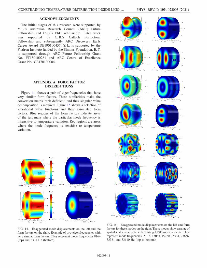
APPENDIX A: FORM FACTORDISTRIBUTIONS

Figure 14 shows a pair of eigenfrequencies that havevery similar form factors. These similarities make theconversion matrix rank deficient, and thus singular valuedecomposition is required. Figure 15 shows a selection ofvibrational wave functions and their associated formfactors. Blue regions of the form factors indicate areasof the test mass where the particular mode frequency isinsensitive to temperature variation. Red regions are areaswhere the mode frequency is sensitive to temperaturevariation.

FIG. 15. Exaggerated mode displacements on the left and formfactors for these modes on the right. These modes show a range ofspatial scales attainable with existing LIGO measurements. Theyrepresent mode frequencies 15016, 15083, 15220, 15534, 23656,33381 and 33610 Hz (top to bottom).

FIG. 14. Exaggerated mode displacements on the left and theform factors on the right. Example of two eigenfrequencies withvery similar form factors. They represent mode frequencies 8164(top) and 8331 Hz (bottom).

CONSTRAINING TEMPERATURE DISTRIBUTION INSIDE LIGO … PHYS. REV. D 103, 022003 (2021)

022003-11

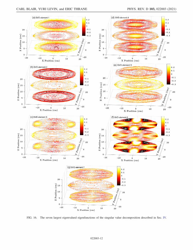
FIG. 16. The seven largest eigenvalued eigenfunctions of the singular value decomposition described in Sec. IV.

CARL BLAIR, YURI LEVIN, and ERIC THRANE PHYS. REV. D 103, 022003 (2021)

022003-12

APPENDIX B: SINGULAR VALUEDECOMPOSITION EIGENFUNCTIONS

Figure 16 shows the first seven singular value decom-position element eigenfunctions for the example give in

Sec. IV. These are the elements with the largest eigen-values and indicate the shapes of temperature distribu-tions most easily recovered from eigenfrequencymeasurements.

[1] J. Aasi et al. (LIGO Scientific Collaboration), ClassicalQuantum Gravity 32, 074001 (2015).

[2] D. V. Martynov, E. D. Hall, B. P. Abbott, R. Abbott,T. D. Abbott, C. Adams, R. X. Adhikari, R. A. Anderson,S. B. Anderson, K. Arai et al., Phys. Rev. D 93, 112004(2016).

[3] A. Buikema, C. Cahillane, G. L. Mansell, C. D. Blair, R.Abbott, C. Adams, R. X. Adhikari, A. Ananyeva, S. Appert,K. Arai et al., Phys. Rev. D 102, 062003 (2020).

[4] G. M. Harry et al. (LIGO Scientific Collaboration),Classical Quantum Gravity 27, 084006 (2010).

[5] A. F. Brooks, B. Abbott, M. A. Arain, G. Ciani, A. Cole, G.Grabeel, E. Gustafson, C. Guido, M. Heintze, A. Hepton-stall et al., Appl. Opt. 55, 8256 (2016).

[6] C. Zhao, J. Degallaix, L. Ju, Y. Fan, D. G. Blair, B. J. J.Slagmolen,M. B.Gray, C.M.MowLowry,D. E.McClelland,D. J. Hosken et al., Phys. Rev. Lett. 96, 231101 (2006).

[7] A. F. Brooks, B. Abbott, M. A. Arain, G. Ciani, A. Cole,G. Grabeel, E. Gustafson, C. Guido, M. Heintze, A.Heptonstall et al., Appl. Opt. 55, 8256 (2016).

[8] V. Braginsky, S. Strigin, and S. Vyatchanin, Phys. Lett. A287, 331 (2001).

[9] C. Zhao, L. Ju, J. Degallaix, S. Gras, and D. G. Blair, Phys.Rev. Lett. 94, 121102 (2005).

[10] C. Blair, S. Gras, R. Abbott, S. Aston, J. Betzwieser, D.Blair, R. DeRosa, M. Evans, V. Frolov, P. Fritschel et al.(LSC Instrument Authors), Phys. Rev. Lett. 118, 151102(2017).

[11] T. Hardwick, V. J. Hamedan, C. Blair, A. C. Green, and D.Vander-Hyde, Classical QuantumGravity 37, 205021 (2020).

[12] H. Wang, C. Blair, M. D. Álvarez, A. Brooks, M. F.Kasprzack, J. Ramette, P. M. Meyers, S. Kaufer, B.O’Reilly, C. M. Mow-Lowry et al., Classical QuantumGravity 34, 115001 (2017).

[13] C. Blair, Ph.D. thesis, University of Western Australia, 35Stirling Hwy, Crawley 6009, Western Australia, 2017,https://doi.org/10.4225/23/59dd76f7f0758.

[14] A. F. Brooks, T.-l. Kelly, P. J. Veitch, and J. Munch, Opt.Express 15, 10370 (2007).

[15] COMSOL, COMSOL Multiphysics version 4.4 (COMSOLInc., BMassachusetts, USA, 2013).

[16] S. Gras, C. Zhao, D. G. Blair, and L. Ju, Classical QuantumGravity 27, 205019 (2010).

[17] S. Biscans, S. Gras, C. D. Blair, J. Driggers, M. Evans, P.Fritschel, T. Hardwick, and G. Mansell, Phys. Rev. D 100,122003 (2019).

[18] Y. Fan, L. Merrill, C. Zhao, L. Ju, D. Blair, B. Slagmolen, D.Hosken, A. Brooks, P. Veitch, and J. Munch, ClassicalQuantum Gravity 27, 084028 (2010).

[19] B. Vladamir, J. Liu, B. Carl, and E. A. Chunnong Zhao (tobe published).

[20] M. Punturo, Technical Report No. VIR-0001A-07 (2007),https://tds.virgo-gw.eu/?content=3&r=1832.

[21] R. Day, V. Fafone, J. Marque, M. Pichot, M. Punturo, and A.Rocchi, Technical Report No. VIR-0191A-10 (2010),https://tds.virgo-gw.eu/?content=3&r=7500.

CONSTRAINING TEMPERATURE DISTRIBUTION INSIDE LIGO … PHYS. REV. D 103, 022003 (2021)

022003-13