102
Physics I experiments By: Atheer Dawood Mahir 2008© 00971503916861 [email protected] POBox 346 , Ajman, UAE
| Date post: | 27-Dec-2015 |
| Category: |
Documents |
| Upload: | edwin-tan-pei-ming |
| View: | 308 times |
| Download: | 11 times |
Physics I experiments
By: Atheer Dawood Mahir
2008© 00971503916861 [email protected]
POBox 346 , Ajman, UAE

Preface II
Preface
Recent welcome changes in practical physics taught in the
University stage have been of two kinds:
(1) the incorporation of new experiments with modern apparatus,
and (2) Computer analysis of experimental data
For the lab course in physics, this text focuses on the useful, hands-
on computer-based skills used day-to-day in implementing an actual
research project. Provides laboratory students with comprehensive
training in data acquisition and analysis by Microsoft excel as
computerized method and by traditional old methods.
Laboratory sessions are designed with a number of outcomes in
mind. We certainly want to investigate many of the concepts and
phenomena that you meet in the lecture part of the course. We also want
you to become proficient in the use of the computer to take and analyze
data and to report the results of your investigations. Learning experimental
techniques and working with each other as you investigate these
phenomena shows you how researchers work together and share ideas.
Thus we will do a variety of things in the lab, which may or may not be
exactly in synch with your class schedule. We want you to act and feel like
researchers - who need to know a variety of skills and information in order
to investigate the world in which they live.
Preface
III
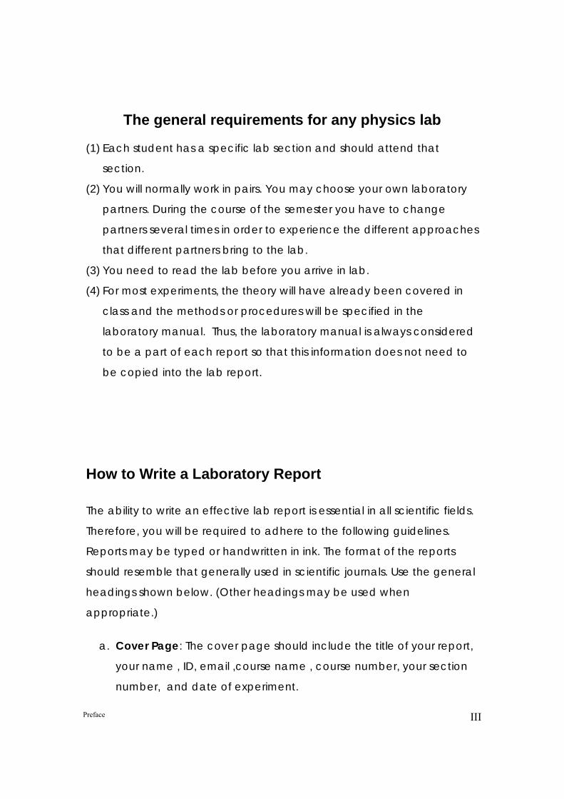
The general requirements for any physics lab
(1) Each student has a specific lab section and should attend that
section.
(2) You will normally work in pairs. You may choose your own laboratory
partners. During the course of the semester you have to change
partners several times in order to experience the different approaches
that different partners bring to the lab.
(3) You need to read the lab before you arrive in lab.
(4) For most experiments, the theory will have already been covered in
class and the methods or procedures will be specified in the
laboratory manual. Thus, the laboratory manual is always considered
to be a part of each report so that this information does not need to
be copied into the lab report.
How to Write a Laboratory Report
The ability to write an effective lab report is essential in all scientific fields.
Therefore, you will be required to adhere to the following guidelines.
Reports may be typed or handwritten in ink. The format of the reports
should resemble that generally used in scientific journals. Use the general
headings shown below. (Other headings may be used when
appropriate.)
a. Cover Page: The cover page should include the title of your report,
your name , ID, email ,course name , course number, your section
number, and date of experiment.
Preface
IV
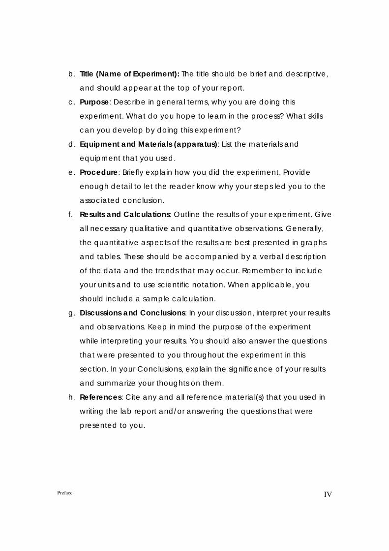
b. Title (Name of Experiment): The title should be brief and descriptive,
and should appear at the top of your report.
c. Purpose: Describe in general terms, why you are doing this
experiment. What do you hope to learn in the process? What skills
can you develop by doing this experiment?
d. Equipment and Materials (apparatus): List the materials and
equipment that you used.
e. Procedure: Briefly explain how you did the experiment. Provide
enough detail to let the reader know why your steps led you to the
associated conclusion.
f. Results and Calculations: Outline the results of your experiment. Give
all necessary qualitative and quantitative observations. Generally,
the quantitative aspects of the results are best presented in graphs
and tables. These should be accompanied by a verbal description
of the data and the trends that may occur. Remember to include
your units and to use scientific notation. When applicable, you
should include a sample calculation.
g. Discussions and Conclusions: In your discussion, interpret your results
and observations. Keep in mind the purpose of the experiment
while interpreting your results. You should also answer the questions
that were presented to you throughout the experiment in this
section. In your Conclusions, explain the significance of your results
and summarize your thoughts on them.
h. References: Cite any and all reference material(s) that you used in
writing the lab report and/or answering the questions that were
presented to you.
Preface
V
Ten laboratory reports in this text are designed with the same divisions
above with some updated requests like links to web, Java, animations,
and photos related to these reports.
As you will see in each practical report, you need to study carefully the
theory and steps of procedure to fill out the Result and Discussion sections.
You need also to prepare graph papers and excel graphs for different
experiment to attach it with result and discussion sections and submit it to
your instructor. You do not need to submit all sections of your report to
correct; just the last two sections (results and discussions) with related
graphs and excel sheets. After correction return it to suitable place to
have a complete report for that experiment.
Atheer Dawood Mahir
Aug.22, 2008, Ajman , UAE
Preface
VI
The contents Preface.................................................................................II
The general requirements for any physics lab .................. III
How to Write a Laboratory Report ................................... III
The contents ...................................................................... III
Significant Digits ............................................................... 3
Graphing Lab and excel ...................................................... 3
Density using different tools............................................... 3
Vectors (free body diagram) ............................................... 3
Motion Along Straight line and Newton's laws .................. 3
Friction................................................................................ 3
Spiral Spring – Hooks Law................................................. 3
Simple Pendulum................................................................ 3
Angular simple harmonic motion ....................................... 3
Moment of inertia ............................................................... 3

Physics Lab AUST
Significant Digits Page 7/102
Experiment 01:
Significant Digits Purpose:
This experiment will demonstrate how to determine the significant digits of a number like(52, 502, 5020, 0.05020, 1.05020) and perform calculations with the correct significant digits:
• The purpose of significant digits. • Determining significant digits • Addition and subtraction • Multiplication and division.
Apparatus : • A support stand with a string
clamp, • Measuring tape, • a stop Watch, • a small spherical ball, • string and scissor, • Transparent ruler , 2 Pencil
(HB) and Eraser • Scientific calculator.
Web:
Significant Figures:
New Theory:
http://www2.wwnorton.com/college/physics/om/_content/_ind
ex/tutorials.shtml (Click on Significant Digits)
http://homepage.mac.com/dtrapp/experiments/SignificantFigur
es.html
http://phoenix.phys.clemson.edu/tutorials/sf/index.html
http://ostermiller.org/calc/sigfig.html
Old Theory:
http://www.ausetute.com.au/sigfig.html
http://www.hazelwood.k12.mo.us/~grichert/sciweb/phys8.htm http://www.chem4free.info/calculators/signdig.htm
Physics Lab AUST
Significant Digits Page 8/102
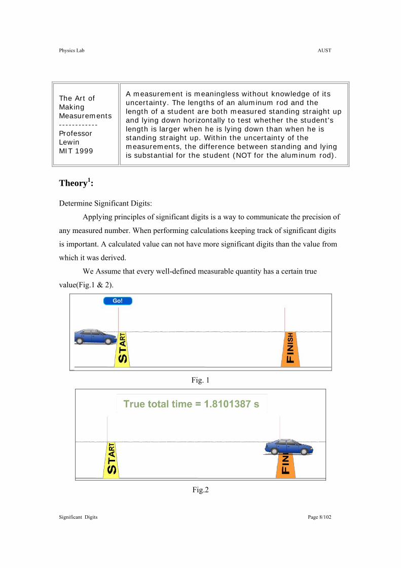
The Art of Making Measurements ------------ Professor Lewin MIT 1999
A measurement is meaningless without knowledge of its uncertainty. The lengths of an aluminum rod and the length of a student are both measured standing straight up and lying down horizontally to test whether the student's length is larger when he is lying down than when he is standing straight up. Within the uncertainty of the measurements, the difference between standing and lying is substantial for the student (NOT for the aluminum rod).
Theory1: Determine Significant Digits:
Applying principles of significant digits is a way to communicate the precision of
any measured number. When performing calculations keeping track of significant digits
is important. A calculated value can not have more significant digits than the value from
which it was derived.
We Assume that every well-defined measurable quantity has a certain true
value(Fig.1 & 2).
Fig. 1
Fig.2
Physics Lab AUST
Significant Digits Page 9/102
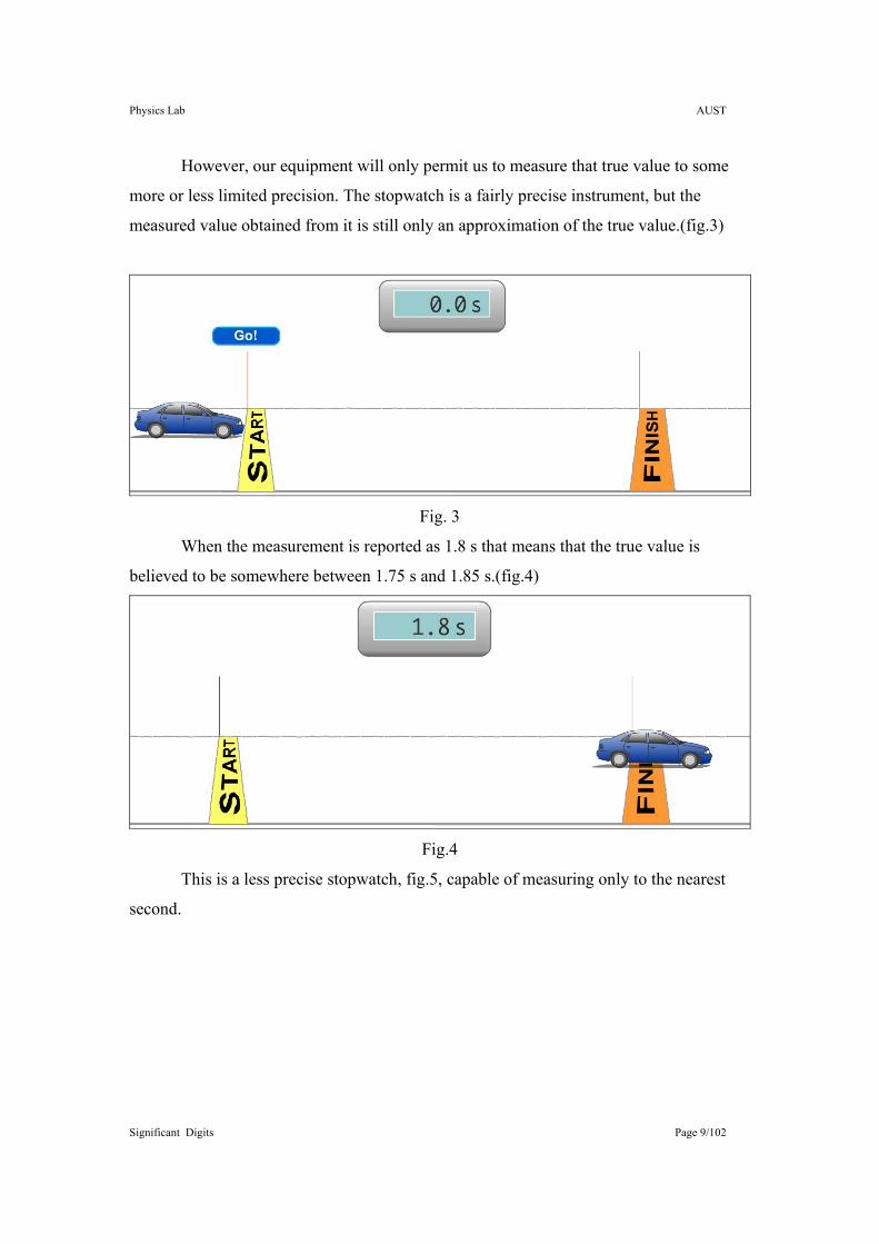
However, our equipment will only permit us to measure that true value to some
more or less limited precision. The stopwatch is a fairly precise instrument, but the
measured value obtained from it is still only an approximation of the true value.(fig.3)
Fig. 3
When the measurement is reported as 1.8 s that means that the true value is
believed to be somewhere between 1.75 s and 1.85 s.(fig.4)
Fig.4
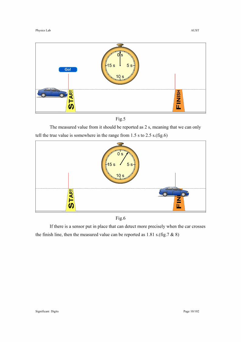
This is a less precise stopwatch, fig.5, capable of measuring only to the nearest
second.
Physics Lab AUST
Significant Digits Page 10/102
Fig.5
The measured value from it should be reported as 2 s, meaning that we can only
tell the true value is somewhere in the range from 1.5 s to 2.5 s.(fig.6)
Fig.6
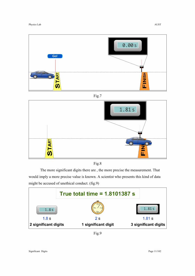
If there is a sensor put in place that can detect more precisely when the car crosses
the finish line, then the measured value can be reported as 1.81 s.(fig.7 & 8)
Physics Lab AUST
Significant Digits Page 11/102
Fig.7
Fig.8
The more significant digits there are , the more precise the measurement. That
would imply a more precise value is known. A scientist who presents this kind of data
might be accused of unethical conduct. (fig.9)
Fig.9
Physics Lab AUST
Significant Digits Page 12/102
When you see a number, it is important to be able to tell how many significant
digits are in it, so that you can tell how much precision is being implied. Numbers can be
written to include non-significant digits as well as significant digits. The following rules
will enable you to tell which digits are the significant ones.
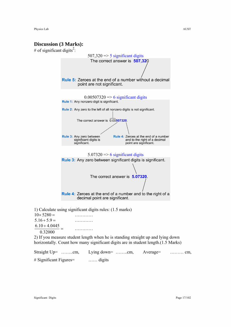
Rule 1: Any nonzero digit is significant.
Rule 2: Any zero to the left of all nonzero digits is not significant.
Rule 3: Any zero between significant digits is significant.
Rule 4: Zeroes at the end of a number and to the right of a decimal point are
significant.
Rule 5: Zeroes at the end of a number without a decimal point are not significant.
Example Significant Digits Rules
52 2 Rule 1
5.03 3 Rule 1,3
5.20 3 Rule 1,4
0.2000 4 Rule 1,2,4
0.0020 2 Rule 1,2,4
52000 2 Rule 1,5
52000.0 6 Rule 1,3,4
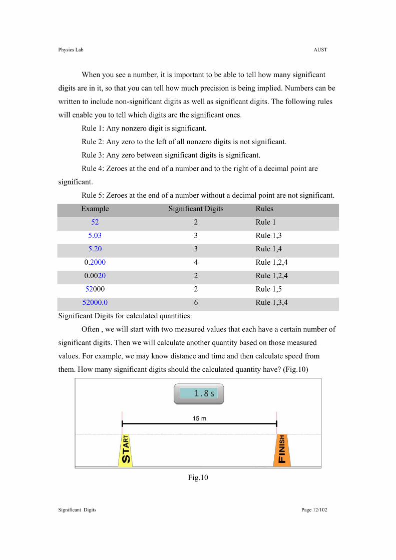
Significant Digits for calculated quantities:
Often , we will start with two measured values that each have a certain number of
significant digits. Then we will calculate another quantity based on those measured
values. For example, we may know distance and time and then calculate speed from
them. How many significant digits should the calculated quantity have? (Fig.10)
Fig.10
Physics Lab AUST
Significant Digits Page 13/102
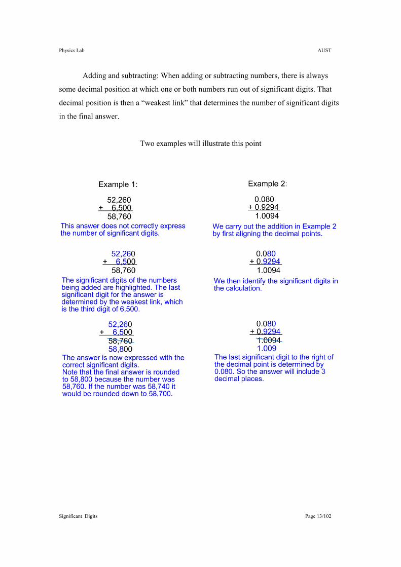
Adding and subtracting: When adding or subtracting numbers, there is always
some decimal position at which one or both numbers run out of significant digits. That
decimal position is then a “weakest link” that determines the number of significant digits
in the final answer.
Two examples will illustrate this point
Physics Lab AUST
Significant Digits Page 14/102
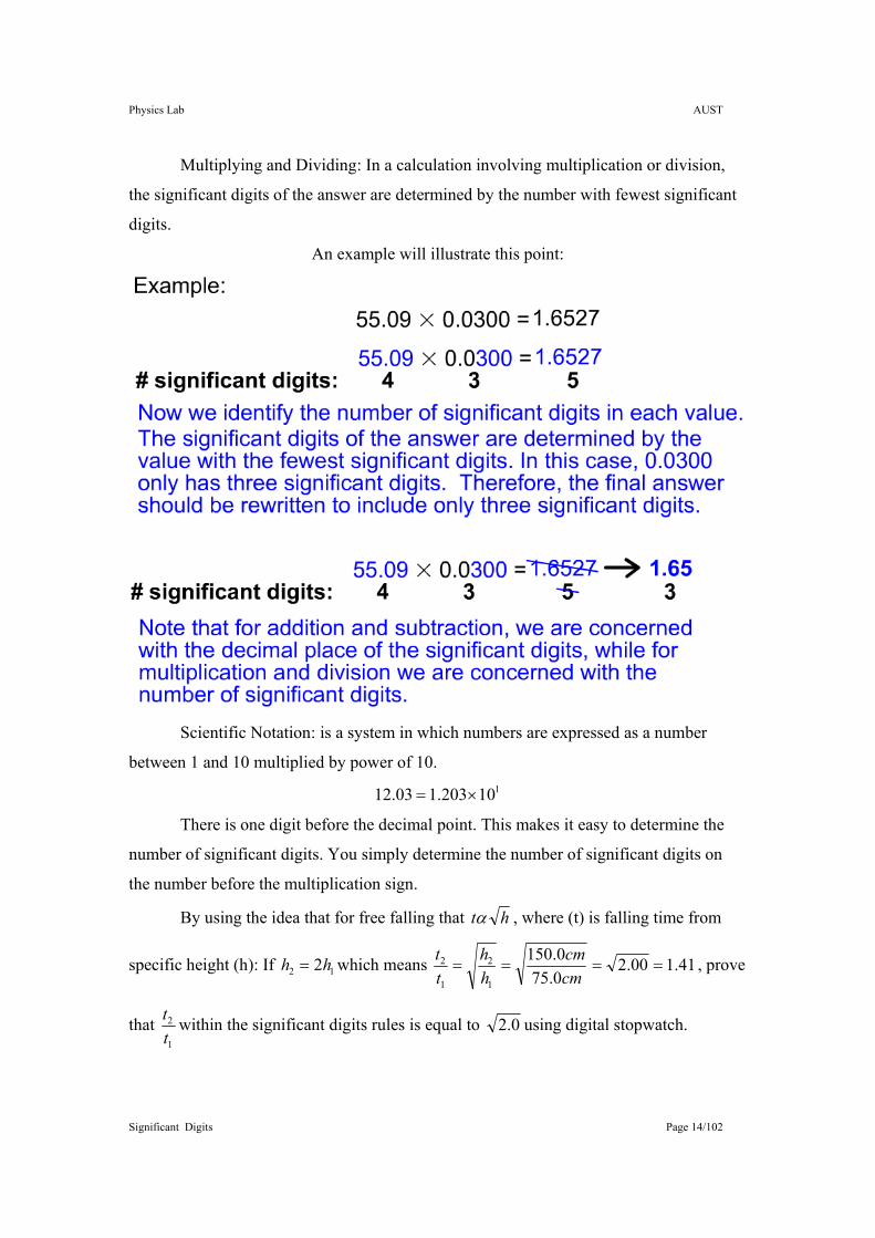
Multiplying and Dividing: In a calculation involving multiplication or division,
the significant digits of the answer are determined by the number with fewest significant
digits.
An example will illustrate this point:
Scientific Notation: is a system in which numbers are expressed as a number
between 1 and 10 multiplied by power of 10. 110203.103.12 ×=
There is one digit before the decimal point. This makes it easy to determine the
number of significant digits. You simply determine the number of significant digits on
the number before the multiplication sign.
By using the idea that for free falling that htα , where (t) is falling time from
specific height (h): If 12 2hh = which means 41.100.20.750.150
1
2
1
2 ====cmcm
hh
tt , prove
that 1
2
tt within the significant digits rules is equal to 0.2 using digital stopwatch.

Physics Lab AUST
Significant Digits Page 15/102
Procedure: 1. Pick small spherical ball suspended by a light string which is attached to a support
stand by a string clamp.
2. Adjust the height of the spherical ball bottom to about 150.0 cm from the ground.
3. Prepare stopwatch and scissor, cut the string and measure falling time using
stopwatch.
4. Repeat previous step for 5 times.
5. Adjust the height of the spherical ball bottom to about 75.0 cm from the ground.
6. Repeat steps 3 & 4.
7. Tabulate your results.
8. Get the significant digits for each measurement.
9. Compare between theoretical result and practical result.
Physics Lab AUST
Significant Digits Page 16/102
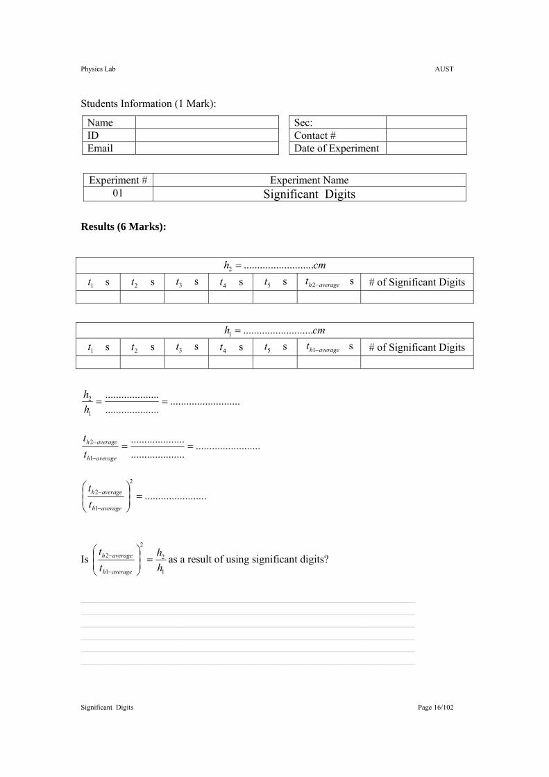
Students Information (1 Mark):
Name Sec: ID Contact # Email Date of Experiment
Experiment # Experiment Name 01 Significant Digits
Results (6 Marks):
cmh ..........................2 =
1t s 2t s 3t s 4t s 5t s averageht −2 s # of Significant Digits
cmh ..........................1 =
1t s 2t s 3t s 4t s 5t s averageht −1 s # of Significant Digits
..................................................................
1
2 ==hh
................................................................
1
2 ==−
−
averageh
averageh
tt
.......................2
1
2 =⎟⎟⎠
⎞⎜⎜⎝
⎛
−
−
averageh
averageh
tt
Is 1
2
2
1
2
hh
tt
averageh
averageh =⎟⎟⎠
⎞⎜⎜⎝
⎛
−
− as a result of using significant digits?
______________________________________________________________ ______________________________________________________________ ______________________________________________________________ ______________________________________________________________ ______________________________________________________________ ______________________________________________________________
Physics Lab AUST
Significant Digits Page 17/102
Discussion (3 Marks): # of significant digits2:
507,320 => 5 significant digits
0.00507320 => 6 significant digits
5.07320 => 6 significant digits
1) Calculate using significant digits rules: (1.5 marks)
=×528010 ………… =+ 9.516.5 …………
=+32000.0
0445.410.6 …………
2) If you measure student length when he is standing straight up and lying down horizontally. Count how many significant digits are in student length.(1.5 Marks) Straight Up= ……..cm, Lying down= ……..cm, Average= ……… cm,
# Significant Figures= …… digits
Physics Lab AUST
Graphing Lab and excel Page 18/102
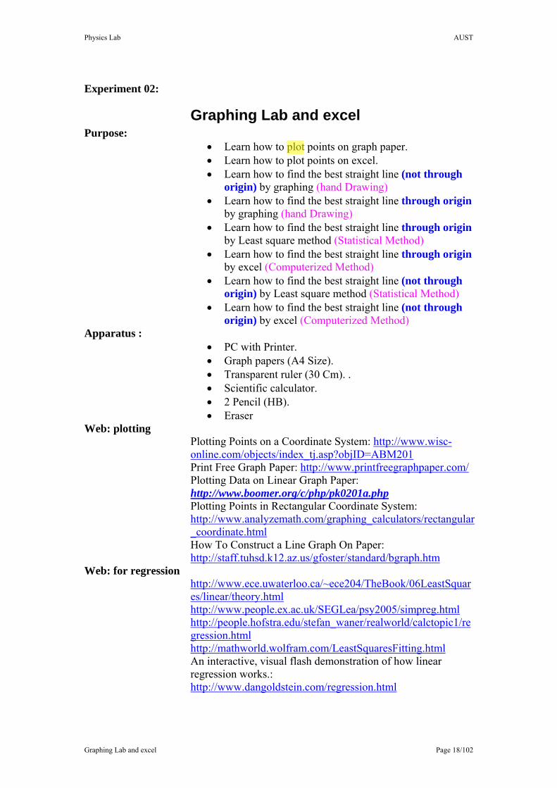
Experiment 02:
Graphing Lab and excel Purpose:
• Learn how to plot points on graph paper. • Learn how to plot points on excel. • Learn how to find the best straight line (not through
origin) by graphing (hand Drawing) • Learn how to find the best straight line through origin
by graphing (hand Drawing) • Learn how to find the best straight line through origin
by Least square method (Statistical Method) • Learn how to find the best straight line through origin
by excel (Computerized Method) • Learn how to find the best straight line (not through
origin) by Least square method (Statistical Method) • Learn how to find the best straight line (not through
origin) by excel (Computerized Method) Apparatus :
• PC with Printer. • Graph papers (A4 Size). • Transparent ruler (30 Cm). . • Scientific calculator. • 2 Pencil (HB). • Eraser
Web: plotting Plotting Points on a Coordinate System: http://www.wisc-online.com/objects/index_tj.asp?objID=ABM201 Print Free Graph Paper: http://www.printfreegraphpaper.com/ Plotting Data on Linear Graph Paper: http://www.boomer.org/c/php/pk0201a.php Plotting Points in Rectangular Coordinate System: http://www.analyzemath.com/graphing_calculators/rectangular_coordinate.html How To Construct a Line Graph On Paper: http://staff.tuhsd.k12.az.us/gfoster/standard/bgraph.htm
Web: for regression http://www.ece.uwaterloo.ca/~ece204/TheBook/06LeastSquares/linear/theory.html http://www.people.ex.ac.uk/SEGLea/psy2005/simpreg.html http://people.hofstra.edu/stefan_waner/realworld/calctopic1/regression.html http://mathworld.wolfram.com/LeastSquaresFitting.html An interactive, visual flash demonstration of how linear regression works.: http://www.dangoldstein.com/regression.html
Physics Lab AUST
Graphing Lab and excel Page 19/102
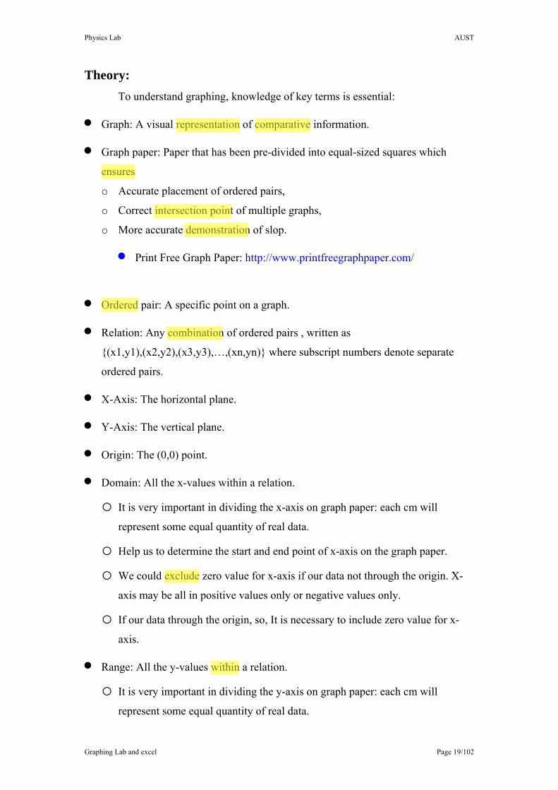
Theory: To understand graphing, knowledge of key terms is essential:
• Graph: A visual representation of comparative information.
• Graph paper: Paper that has been pre-divided into equal-sized squares which
ensures
o Accurate placement of ordered pairs,
o Correct intersection point of multiple graphs,
o More accurate demonstration of slop.
• Print Free Graph Paper: http://www.printfreegraphpaper.com/
• Ordered pair: A specific point on a graph.
• Relation: Any combination of ordered pairs , written as
{(x1,y1),(x2,y2),(x3,y3),…,(xn,yn)} where subscript numbers denote separate
ordered pairs.
• X-Axis: The horizontal plane.
• Y-Axis: The vertical plane.
• Origin: The (0,0) point.
• Domain: All the x-values within a relation.
o It is very important in dividing the x-axis on graph paper: each cm will
represent some equal quantity of real data.
o Help us to determine the start and end point of x-axis on the graph paper.
o We could exclude zero value for x-axis if our data not through the origin. X-
axis may be all in positive values only or negative values only.
o If our data through the origin, so, It is necessary to include zero value for x-
axis.
• Range: All the y-values within a relation.
o It is very important in dividing the y-axis on graph paper: each cm will
represent some equal quantity of real data.
Physics Lab AUST
Graphing Lab and excel Page 20/102
o Help us to determine the start and end point of y-axis on the graph paper.
o We could exclude zero value for y-axis if our data not through the origin. Y-
axis may be all in positive values only or negative values only.
o If our data through the origin, so, It is necessary to include zero value for y-
axis.
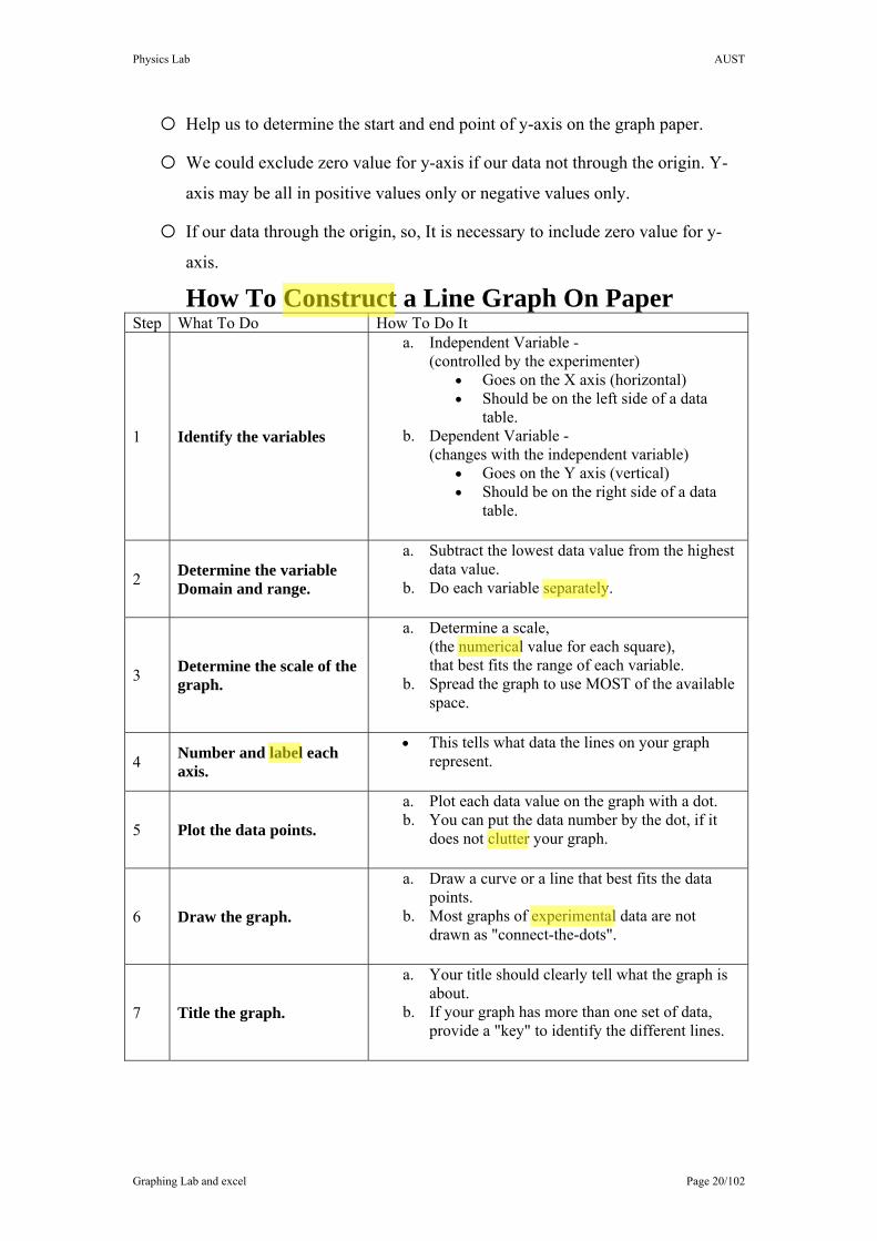
How To Construct a Line Graph On Paper Step What To Do How To Do It
1 Identify the variables
a. Independent Variable - (controlled by the experimenter)
• Goes on the X axis (horizontal) • Should be on the left side of a data
table. b. Dependent Variable -
(changes with the independent variable) • Goes on the Y axis (vertical) • Should be on the right side of a data
table.
2 Determine the variable Domain and range.
a. Subtract the lowest data value from the highest data value.
b. Do each variable separately.
3 Determine the scale of the graph.
a. Determine a scale, (the numerical value for each square), that best fits the range of each variable.
b. Spread the graph to use MOST of the available space.
4 Number and label each axis.
• This tells what data the lines on your graph represent.
5 Plot the data points.
a. Plot each data value on the graph with a dot. b. You can put the data number by the dot, if it
does not clutter your graph.
6 Draw the graph.
a. Draw a curve or a line that best fits the data points.
b. Most graphs of experimental data are not drawn as "connect-the-dots".
7 Title the graph.
a. Your title should clearly tell what the graph is about.
b. If your graph has more than one set of data, provide a "key" to identify the different lines.
Physics Lab AUST
Graphing Lab and excel Page 21/102
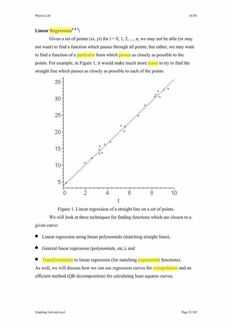
Linear Regression3 4 5:
Given a set of points (xi, yi) for i = 0, 1, 2, ..., n, we may not be able (or may
not want) to find a function which passes through all points, but rather, we may want
to find a function of a particular form which passes as closely as possible to the
points. For example, in Figure 1, it would make much more sense to try to find the
straight line which passes as closely as possible to each of the points.
Figure 1. Linear regression of a straight line on a set of points.
We will look at three techniques for finding functions which are closest to a
given curve:
• Linear regression using linear polynomials (matching straight lines),
• General linear regression (polynomials, etc.), and
• Transformations to linear regression (for matching exponential functions).
As well, we will discuss how we can use regression curves for extrapolation and an
efficient method (QR decomposition) for calculating least squares curves.
Physics Lab AUST
Graphing Lab and excel Page 22/102
Terminology:
This processes is called regression because the y values are regressing (or
moving towards) the value on the curve which we find.
The term linear in linear regression refers to the coefficients of the matching
function. As a special case, we begin by looking at linear regression using linear
polynomials (i.e., y = ax + b).
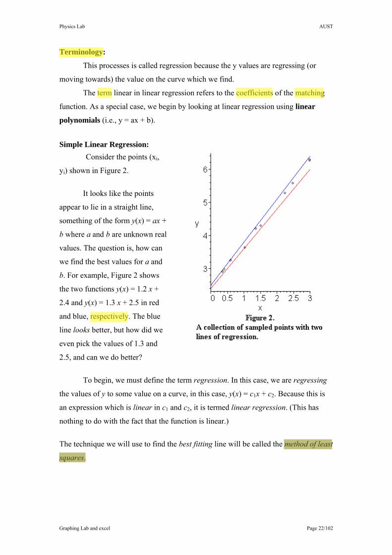
Simple Linear Regression:
Consider the points (xi,
yi) shown in Figure 2.
It looks like the points
appear to lie in a straight line,
something of the form y(x) = ax +
b where a and b are unknown real
values. The question is, how can
we find the best values for a and
b. For example, Figure 2 shows
the two functions y(x) = 1.2 x +
2.4 and y(x) = 1.3 x + 2.5 in red
and blue, respectively. The blue
line looks better, but how did we
even pick the values of 1.3 and
2.5, and can we do better?
To begin, we must define the term regression. In this case, we are regressing
the values of y to some value on a curve, in this case, y(x) = c1x + c2. Because this is
an expression which is linear in c1 and c2, it is termed linear regression. (This has
nothing to do with the fact that the function is linear.)
The technique we will use to find the best fitting line will be called the method of least
squares.
Physics Lab AUST
Graphing Lab and excel Page 23/102
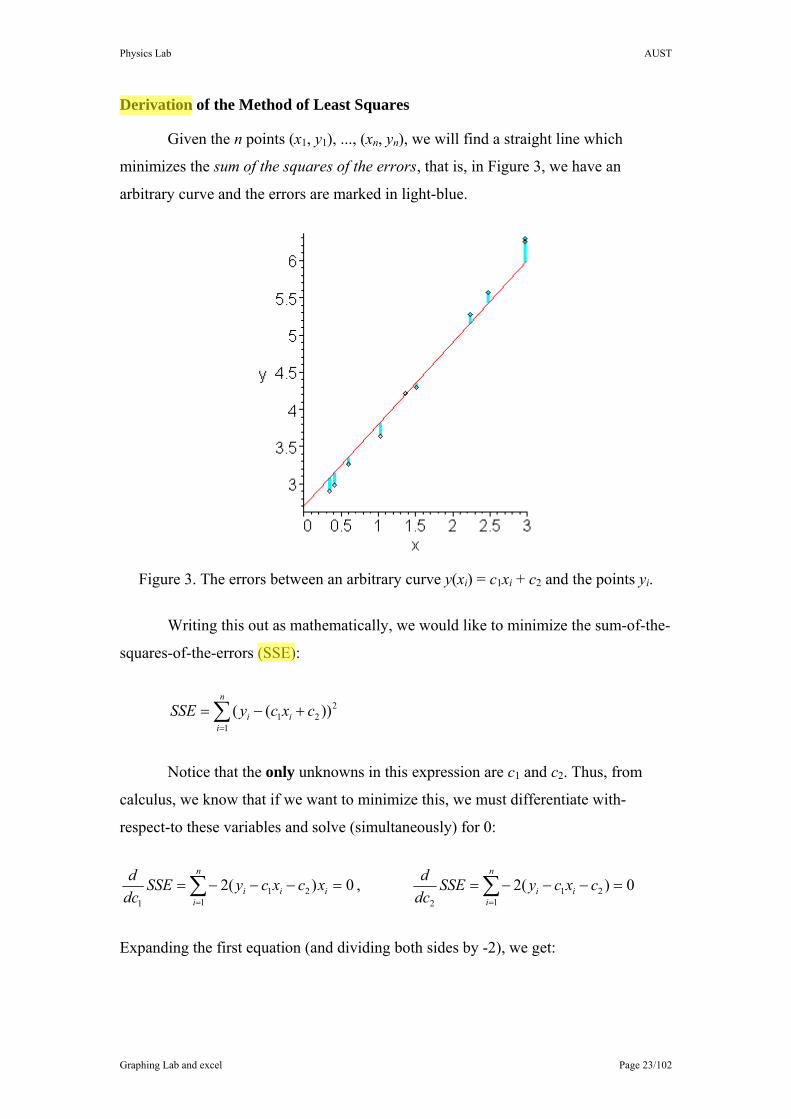
Derivation of the Method of Least Squares
Given the n points (x1, y1), ..., (xn, yn), we will find a straight line which
minimizes the sum of the squares of the errors, that is, in Figure 3, we have an
arbitrary curve and the errors are marked in light-blue.
Figure 3. The errors between an arbitrary curve y(xi) = c1xi + c2 and the points yi.
Writing this out as mathematically, we would like to minimize the sum-of-the-
squares-of-the-errors (SSE):
∑=
+−=n
iii cxcySSE
1
221 ))((
Notice that the only unknowns in this expression are c1 and c2. Thus, from
calculus, we know that if we want to minimize this, we must differentiate with-
respect-to these variables and solve (simultaneously) for 0:
0)(21
211
=−−−= ∑=
n
iiii xcxcySSE
dcd , 0)(2
121
2
=−−−= ∑=
n
iii cxcySSE
dcd
Expanding the first equation (and dividing both sides by -2), we get:

Physics Lab AUST
Graphing Lab and excel Page 24/102
01
21
21
1=−− ∑∑∑
===
n
ii
n
ii
n
iii xcxcyx
If we, with some foresight, define the following, the sum of the x's (Sx), the sum of the
y's (Sy), the sum of the squares of the x's (SSy), and the sum of the products of the x's
and y's (SPx, y), that is,
∑∑∑∑====
====n
iiiyx
n
iix
n
iiy
n
iix yxSPxSSySxS
1,
1
2
11
,,,
the we get the linear equation:
yxxx SPcScSS ,21 =+
Expanding the second equation (and dividing both sides by -2), we get:
011
21
11
=−− ∑∑∑===
n
i
n
ii
n
ii cxcy
By calculating the third sum and rearranging, we get the linear equation:
yx SnccS =+ 21
We could solve these the long way (as you probably did in high school), however, we
note that this describes the system of equations:
⎟⎟⎠
⎞⎜⎜⎝
⎛=⎟⎟
⎠
⎞⎜⎜⎝
⎛⎟⎟⎠
⎞⎜⎜⎝
⎛
y
yx
x
xx
SSP
cc
nSSSS ,
2
1 , this is a system of linear equations which we can, quite
easily, solve.
⎪⎪⎪⎪⎪⎪
⎭
⎪⎪⎪⎪⎪⎪
⎬
⎫
⎪⎪⎪⎪⎪⎪
⎩
⎪⎪⎪⎪⎪⎪
⎨
⎧
⎟⎠
⎞⎜⎝
⎛−⎟
⎠
⎞⎜⎝
⎛
==
⎟⎠
⎞⎜⎝
⎛−⎟⎠
⎞⎜⎝
⎛
⎟⎠
⎞⎜⎝
⎛⎟⎠
⎞⎜⎝
⎛−⎟
⎠
⎞⎜⎝
⎛
==
⎪⎭
⎪⎬
⎫
+=
==
∑∑
∑∑
∑∑∑
==
==
===
n
xayb
xxn
yxyx
baxy
cbcaFitBest
n
ii
n
ii
n
ii
n
ii
n
ii
n
ii
n
iii
11
2
11
2
111
21
intercept
nslopea
where So
,, :
…..(1)
Physics Lab AUST
Graphing Lab and excel Page 25/102
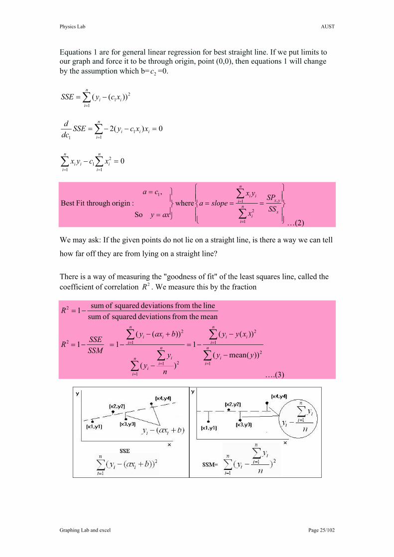
Equations 1 are for general linear regression for best straight line. If we put limits to our graph and force it to be through origin, point (0,0), then equations 1 will change by the assumption which b= 2c =0.
∑=
−=n
iii xcySSE
1
21 ))((
0)(21
11
=−−= ∑=
n
iiii xxcySSE
dcd
01
21
1=− ∑∑
==
n
ii
n
iii xcyx
⎪⎪⎭
⎪⎪⎬
⎫
⎪⎪⎩
⎪⎪⎨
⎧
===⎪⎭
⎪⎬
⎫
=
=
∑
∑
=
=
x
yxn
ii
n
iii
SSSP
x
yxslopea
axy
ca,
1
2
11
where So
, :originh Fit througBest
…(2)
We may ask: If the given points do not lie on a straight line, is there a way we can tell
how far off they are from lying on a straight line?
There is a way of measuring the "goodness of fit" of the least squares line, called the coefficient of correlation 2R . We measure this by the fraction
∑
∑
∑∑
∑
=
=
=
=
=
−
−−=
−
+−−=−=
−=
n
ii
n
iii
n
i
n
ii
i
n
iii
yy
xyy
n
yy
baxy
SSMSSER
R
1
2
1
2
1
21
1
2
2
2
))(mean(
))((1
)(
))((1 1
mean thefrom deviations squared of sumline thefrom deviations squared of sum1
….(3)
Physics Lab AUST
Graphing Lab and excel Page 26/102
Procedure: A. These are readings of some experiments, please use your hand to plot these points on two separated graph paper , then , draw the best straight line (not through the origin) for the first graph and best straight line through origin for the next graph.
According to How To Construct a Line Graph On Paper o Independent Variable is X , Dependent Variable is V o Variable Domain=10-2=8 m, Range=23.5-7.1=16.4~17 m/s o Scales :
o X-scale: (1 m) for each (2cm) on the graph paper ~ need at least 8*2cm=16 cm x-axis.
o Y-scale: (1 m/s) for each (1cm) on the graph paper~ need at least 17*1cm=17 cm y-axis.
o Number and label each axis, Plot the data points and Draw a line that best fits the data points.
o Title the graph.
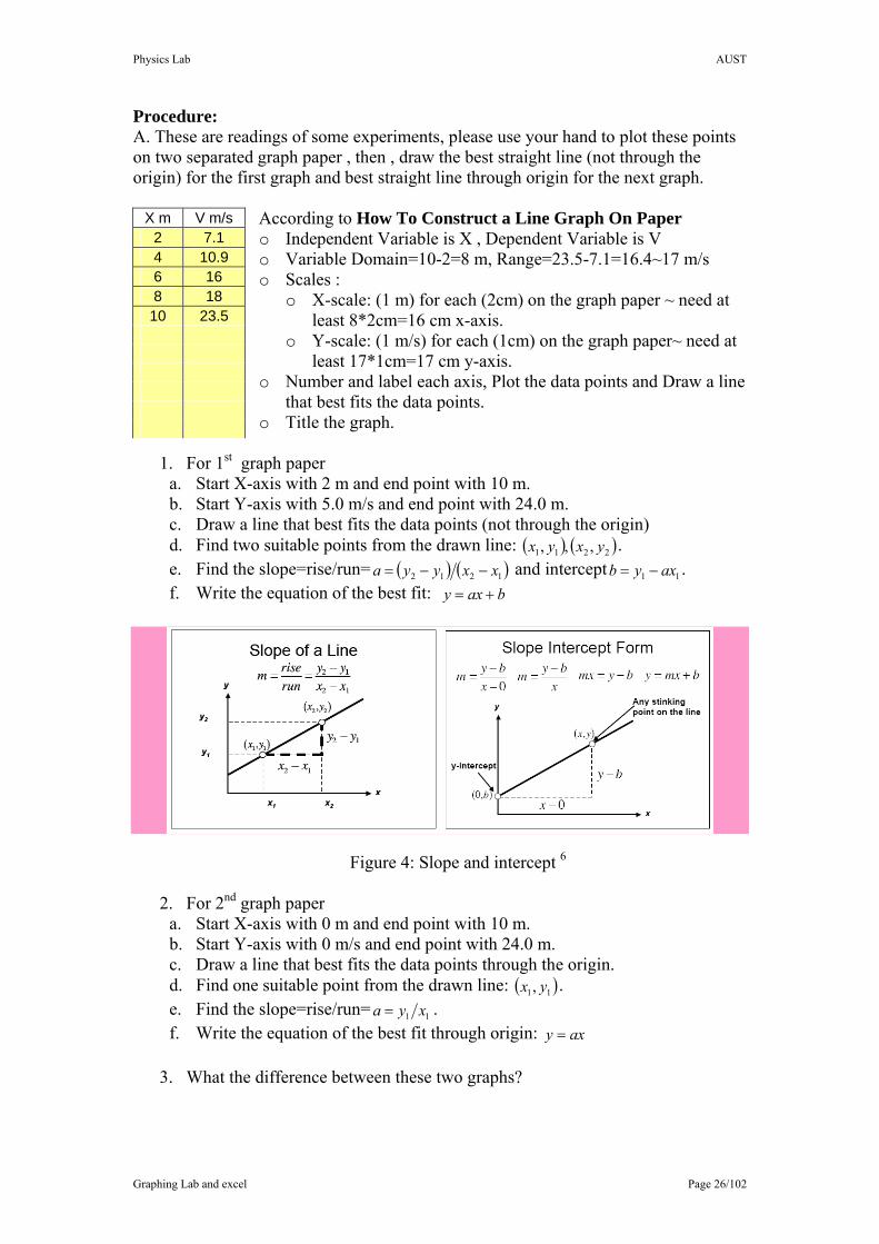
1. For 1st graph paper a. Start X-axis with 2 m and end point with 10 m. b. Start Y-axis with 5.0 m/s and end point with 24.0 m. c. Draw a line that best fits the data points (not through the origin) d. Find two suitable points from the drawn line: ( ) ( )2211 , ,, yxyx . e. Find the slope=rise/run= ( ) ( )1212 xxyya −−= and intercept 11 axyb −= . f. Write the equation of the best fit: baxy +=
Figure 4: Slope and intercept 6
2. For 2nd graph paper a. Start X-axis with 0 m and end point with 10 m. b. Start Y-axis with 0 m/s and end point with 24.0 m. c. Draw a line that best fits the data points through the origin. d. Find one suitable point from the drawn line: ( )11, yx . e. Find the slope=rise/run= 11 xya = . f. Write the equation of the best fit through origin: axy =
3. What the difference between these two graphs?
X m V m/s 2 7.1 4 10.9 6 16 8 18
10 23.5
Physics Lab AUST
Graphing Lab and excel Page 27/102
B. Make the graph papers, but now use the statistical equations 1, 2, 3 1. For 3rd graph paper
a. Start X-axis with 2.0 m and end point with 10 m. b. Start Y-axis with 5.0 m/s and end point with 24.0 m. c. Use equations 1 to find the equation for the best fitting line. d. Draw a line that best fits the data points by selecting two values of x from x-
axis values. Let 9 ,3 21 == xx and find ? ?, 21 == yy . e. Draw these two points ( ) ( )2211 , ,, yxyx on the graph paper to draw the line
through them which is representing the equation of best fit. f. Compare it with 1st graph of section A. g. Find the coefficient of correlation 2R .
2. For 4th graph paper
a. Start X-axis with 0 m and end point with 10 m. b. Start Y-axis with 0 m/s and end point with 24.0 m. c. Use equation 2 to find the equation for the best fitting line through origin. d. Draw a line that best fits the data points by selecting one value of x from x-
axis values. Let 71 =x and find ?1 =y . e. Draw these two points ( ) ( )11, ,0,0 yx on the graph paper to draw the line
through them which is representing the equation of best fit through origin. f. Compare it with 2nd graph of section A. g. Find the coefficient of correlation 2R .
3. What the difference between these two graphs (3rd and 4th) according to
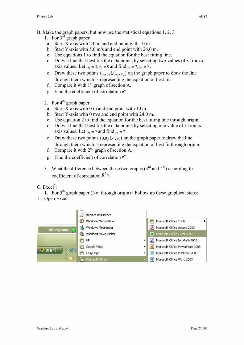
coefficient of correlation 2R ? C. Excel7:
1. For 5th graph paper (Not through origin) : Follow up these graphical steps: 1. Open Excel:
Physics Lab AUST
Graphing Lab and excel Page 28/102
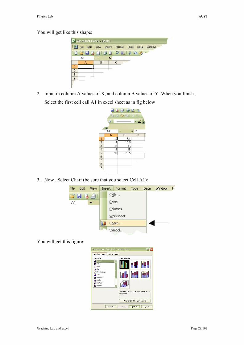
You will get like this shape:
2. Input in column A values of X, and column B values of Y. When you finish ,
Select the first cell call A1 in excel sheet as in fig below
3. Now , Select Chart (be sure that you select Cell A1):
You will get this figure:
Physics Lab AUST
Graphing Lab and excel Page 29/102
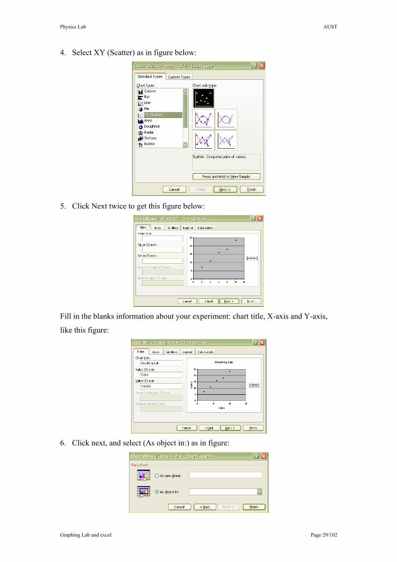
4. Select XY (Scatter) as in figure below:
5. Click Next twice to get this figure below:
Fill in the blanks information about your experiment: chart title, X-axis and Y-axis,
like this figure:
6. Click next, and select (As object in:) as in figure:
Physics Lab AUST
Graphing Lab and excel Page 30/102
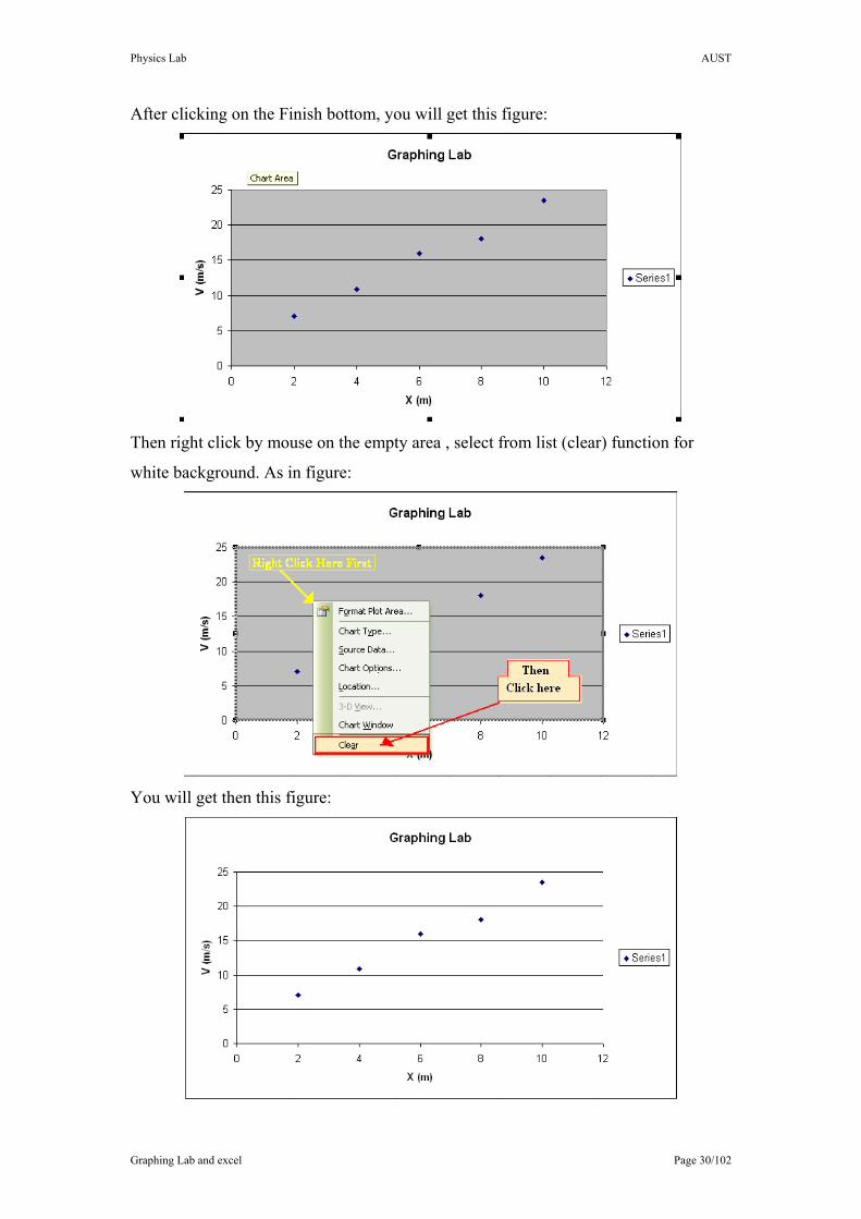
After clicking on the Finish bottom, you will get this figure:
Then right click by mouse on the empty area , select from list (clear) function for
white background. As in figure:
You will get then this figure:
Physics Lab AUST
Graphing Lab and excel Page 31/102
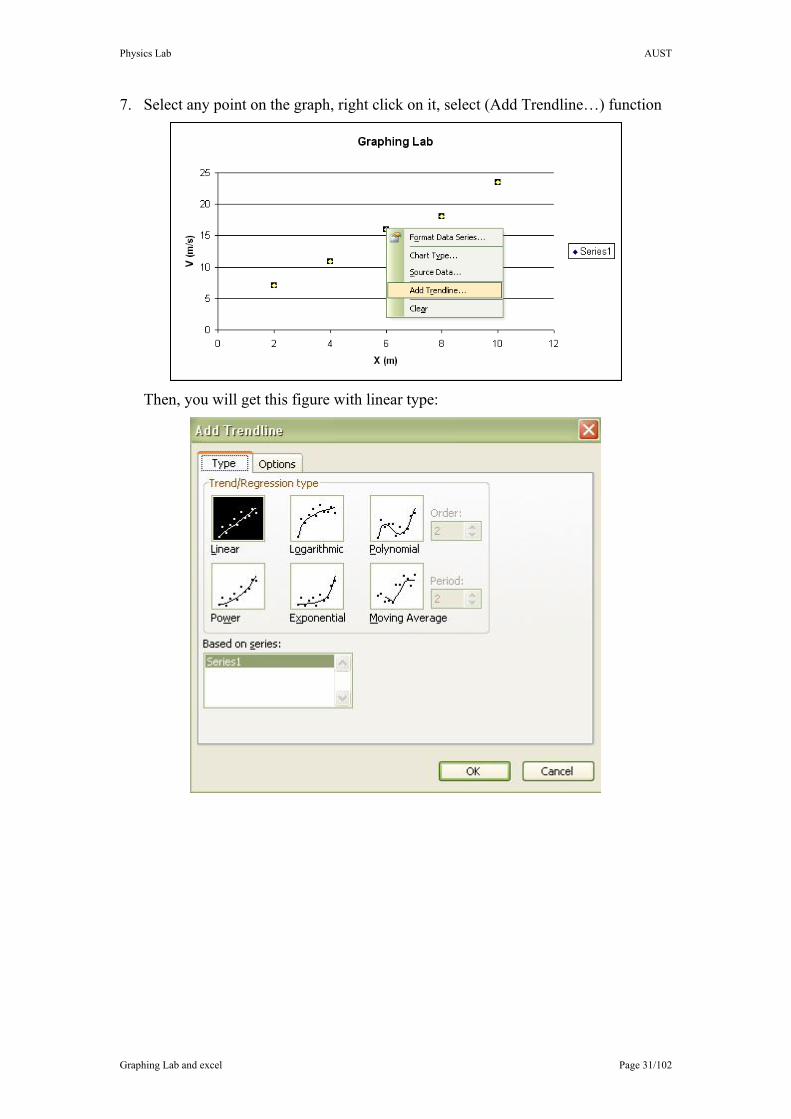
7. Select any point on the graph, right click on it, select (Add Trendline…) function
Then, you will get this figure with linear type:
Physics Lab AUST
Graphing Lab and excel Page 32/102
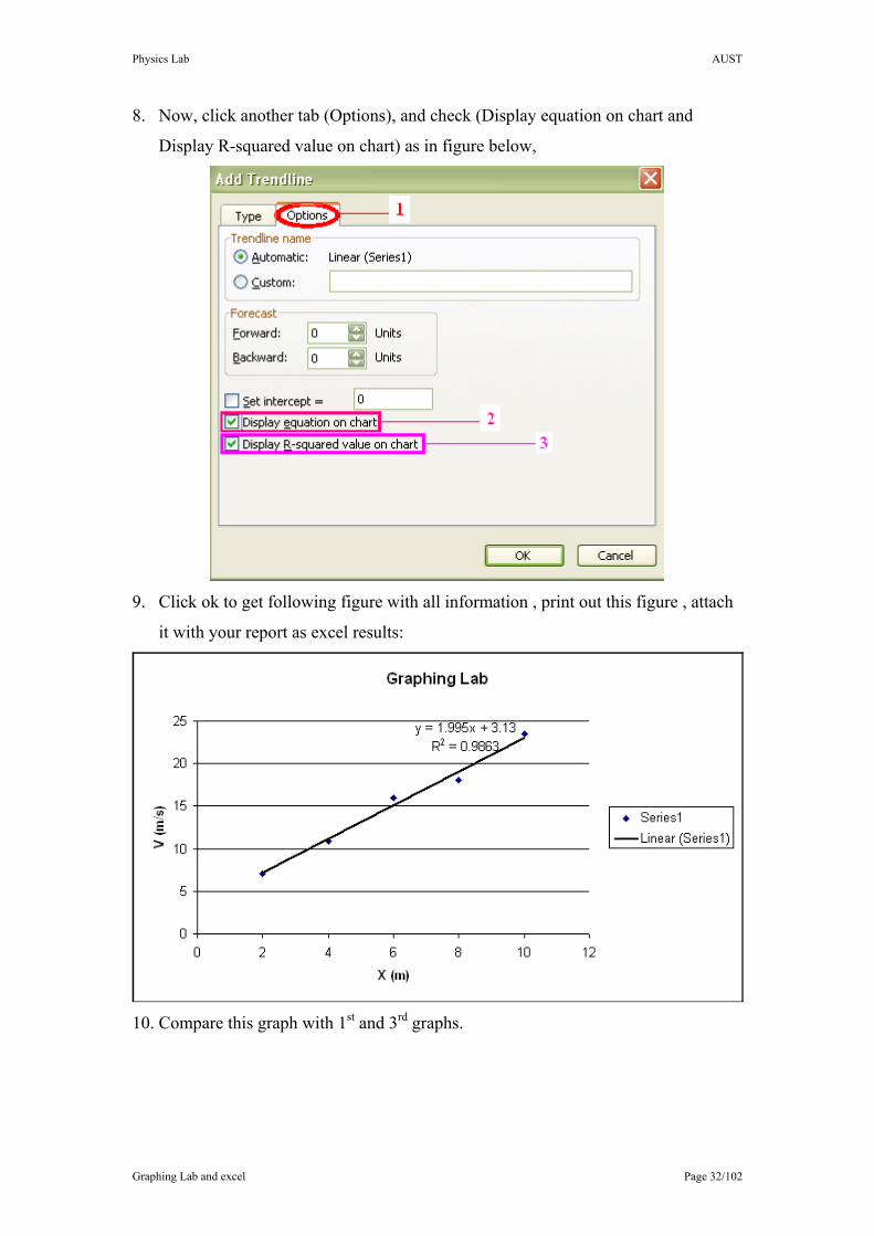
8. Now, click another tab (Options), and check (Display equation on chart and
Display R-squared value on chart) as in figure below,
9. Click ok to get following figure with all information , print out this figure , attach
it with your report as excel results:
10. Compare this graph with 1st and 3rd graphs.
Physics Lab AUST
Graphing Lab and excel Page 33/102
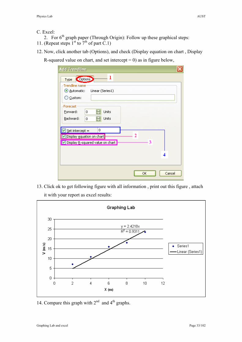
C. Excel: 2. For 6th graph paper (Through Origin): Follow up these graphical steps:
11. (Repeat steps 1st to 7th of part C.1)
12. Now, click another tab (Options), and check (Display equation on chart , Display
R-squared value on chart, and set intercept = 0) as in figure below,
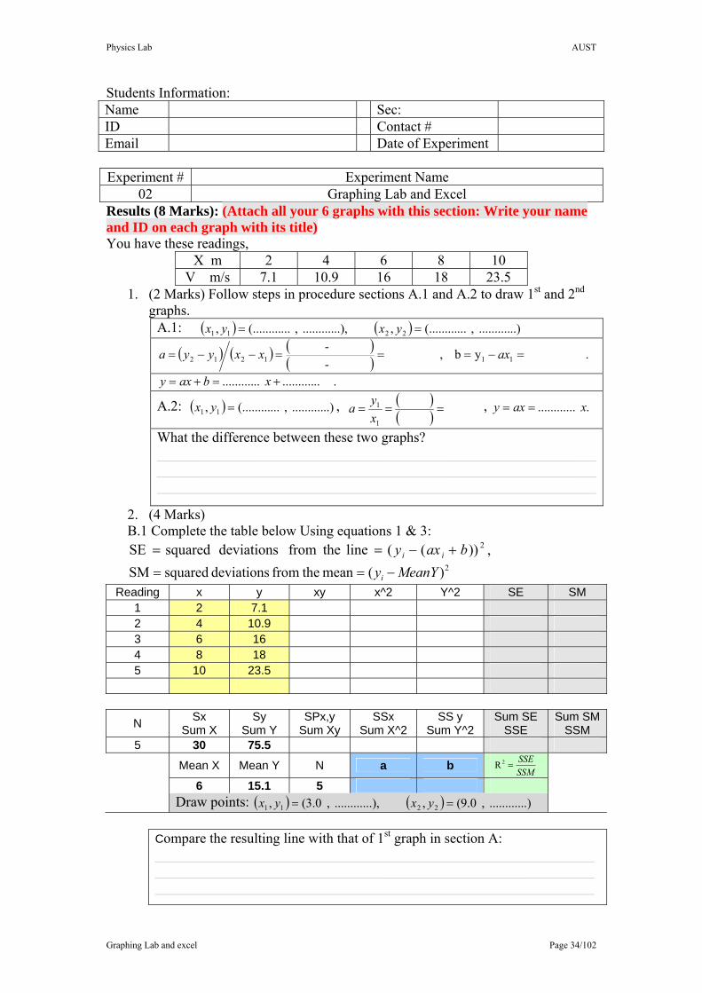
13. Click ok to get following figure with all information , print out this figure , attach
it with your report as excel results:
14. Compare this graph with 2nd and 4th graphs.
Physics Lab AUST
Graphing Lab and excel Page 34/102
Students Information: Name Sec: ID Contact # Email Date of Experiment Experiment # Experiment Name
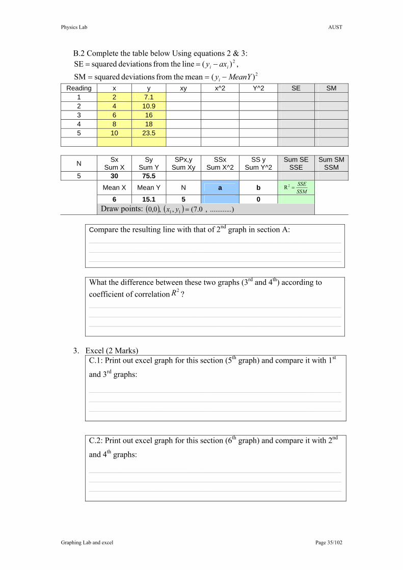
02 Graphing Lab and Excel Results (8 Marks): (Attach all your 6 graphs with this section: Write your name and ID on each graph with its title) You have these readings,
X m 2 4 6 8 10 V m/s 7.1 10.9 16 18 23.5
1. (2 Marks) Follow steps in procedure sections A.1 and A.2 to draw 1st and 2nd graphs.
A.1: ( ) ( ) ..).......... , ...(........., ..),.......... , ...(........., 2211 == yxyx
( ) ( ) ( )( ) . yb ,
- -
111212 =−===−−= axxxyya
. ............ ............ +=+= xbaxy
A.2: ( ) ..).......... , ...(........., 11 =yx , ( )( )
1
1 ===xya , . ............ xaxy ==
What the difference between these two graphs? ______________________________________________________________ ______________________________________________________________ ______________________________________________________________
2. (4 Marks) B.1 Complete the table below Using equations 1 & 3:
2))((line thefrom deviations squaredSE baxy ii +−== , 2)(mean thefrom deviations squaredSM MeanYyi −==
Reading x y xy x^2 Y^2 SE SM 1 2 7.1 2 4 10.9 3 6 16 4 8 18 5 10 23.5
N Sx Sum X
Sy Sum Y
SPx,y Sum Xy
SSx Sum X^2
SS y Sum Y^2
Sum SE SSE
Sum SM SSM
5 30 75.5 Mean X Mean Y N a b SSM
SSE=2R
6 15.1 5 Draw points: ( ) ( ) ..).......... , 0.9(, ..),.......... , 0.3(, 2211 == yxyx
Compare the resulting line with that of 1st graph in section A: ______________________________________________________________ ______________________________________________________________ ______________________________________________________________
Physics Lab AUST
Graphing Lab and excel Page 35/102
B.2 Complete the table below Using equations 2 & 3: 2)(line thefrom deviations squaredSE ii axy −== ,
2)(mean thefrom deviations squaredSM MeanYyi −== Reading x y xy x^2 Y^2 SE SM
1 2 7.1 2 4 10.9 3 6 16 4 8 18 5 10 23.5
N Sx Sum X
Sy Sum Y
SPx,y Sum Xy
SSx Sum X^2
SS y Sum Y^2
Sum SE SSE
Sum SM SSM
5 30 75.5 Mean X Mean Y N a b SSM
SSE=2R
6 15.1 5 0 Draw points: ( ) ( ) ..).......... , 0.7(, ,0,0 11 =yx
Compare the resulting line with that of 2nd graph in section A: __________________________________________________________________________________________________________________________________________________________________________________________
What the difference between these two graphs (3rd and 4th) according to coefficient of correlation 2R ? __________________________________________________________________________________________________________________________________________________________________________________________
3. Excel (2 Marks)
C.1: Print out excel graph for this section (5th graph) and compare it with 1st
and 3rd graphs:
______________________________________________________________ ______________________________________________________________ ______________________________________________________________
C.2: Print out excel graph for this section (6th graph) and compare it with 2nd
and 4th graphs:
______________________________________________________________ ______________________________________________________________ ______________________________________________________________

Physics Lab AUST
Graphing Lab and excel Page 36/102
Discussion (2 Marks):
1. What you learn from this lab:
______________________________________________________________ ______________________________________________________________ ______________________________________________________________ ______________________________________________________________ ______________________________________________________________ ______________________________________________________________ ______________________________________________________________ ______________________________________________________________ ______________________________________________________________ ______________________________________________________________ ______________________________________________________________ ______________________________________________________________ ______________________________________________________________ ______________________________________________________________
2. What are you prefer, excel or statistical or hand drawing? why?
______________________________________________________________ ______________________________________________________________ ______________________________________________________________ ______________________________________________________________ ______________________________________________________________ ______________________________________________________________ ______________________________________________________________ ______________________________________________________________ ______________________________________________________________
Physics Lab AUST
Density using different tools Page 37/102
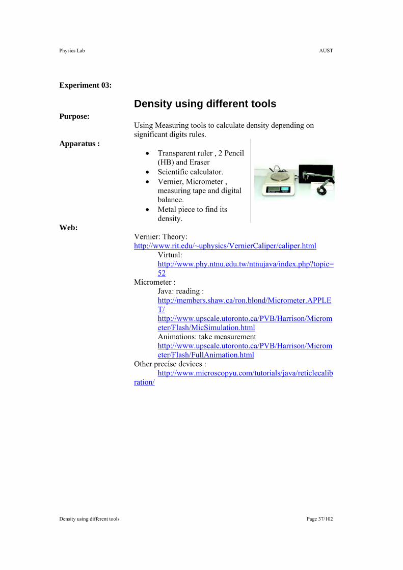
Experiment 03:
Density using different tools Purpose:
Using Measuring tools to calculate density depending on significant digits rules.
Apparatus : • Transparent ruler , 2 Pencil
(HB) and Eraser • Scientific calculator. • Vernier, Micrometer ,
measuring tape and digital balance.
• Metal piece to find its density.
Web: Vernier: Theory: http://www.rit.edu/~uphysics/VernierCaliper/caliper.html
Virtual: http://www.phy.ntnu.edu.tw/ntnujava/index.php?topic=52
Micrometer : Java: reading : http://members.shaw.ca/ron.blond/Micrometer.APPLET/ http://www.upscale.utoronto.ca/PVB/Harrison/Micrometer/Flash/MicSimulation.html Animations: take measurement http://www.upscale.utoronto.ca/PVB/Harrison/Micrometer/Flash/FullAnimation.html
Other precise devices : http://www.microscopyu.com/tutorials/java/reticlecalibration/
Physics Lab AUST
Density using different tools Page 38/102
Theory8:
Accuracies of measuring tools are 0.1 cm , 0.01 cm, 0.001 cm for ruler , vernier
and micrometer, respectively.
In a engineering laboratory it is often necessary to determine the length and
masses of objects. Sometime it is necessary to do this with some degree of precision.
Various measuring tools exist for performing such measurements, such as vernier
callipers, micrometers, dial gauges. These instruments are capable of giving very precise
answers, provided the instruments are used with some degree of care.
In this experiment, you will be given a metal sample. You will then take readings
of its spatial dimensions. From these reading you will then determine a value of the mass
of the sample which you will confirm using an electronic balance.
We will describe the operation of a vernier calliper, a micrometer and a dial gauge
(Optional Device). Once you have read the section, the specific experiments that you
perform will be described.
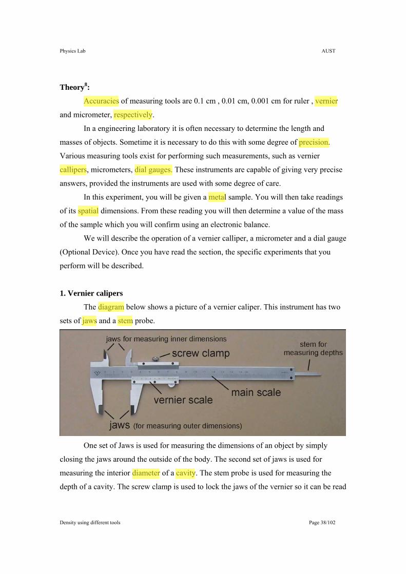
1. Vernier calipers
The diagram below shows a picture of a vernier caliper. This instrument has two
sets of jaws and a stem probe.
One set of Jaws is used for measuring the dimensions of an object by simply
closing the jaws around the outside of the body. The second set of jaws is used for
measuring the interior diameter of a cavity. The stem probe is used for measuring the
depth of a cavity. The screw clamp is used to lock the jaws of the vernier so it can be read
Physics Lab AUST
Density using different tools Page 39/102
without modifying the position of the sliding scale. The precision of length measurements
may be increased by using a device that uses a sliding vernier scale. This instrument has a
main scale (in millimetres) and a sliding vernier scale. In figure 1 below, the vernier scale
(below) is divided into 10 equal divisions and thus the highest precision of the instrument
is 0.1 mm (note, some calipers have a scales giving a precision of 0.02 mm). Both the
main scale and the vernier scale readings are taken into account while making a
measurement. The main scale reading is given by the position of the zero mark on the
sliding vernier.
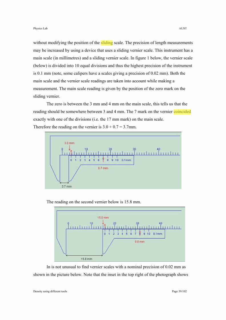
The zero is between the 3 mm and 4 mm on the main scale, this tells us that the
reading should be somewhere between 3 and 4 mm. The 7 mark on the vernier coincided
exactly with one of the divisions (i.e. the 17 mm mark) on the main scale.
Therefore the reading on the vernier is 3.0 + 0.7 = 3.7mm.
The reading on the second vernier below is 15.8 mm.
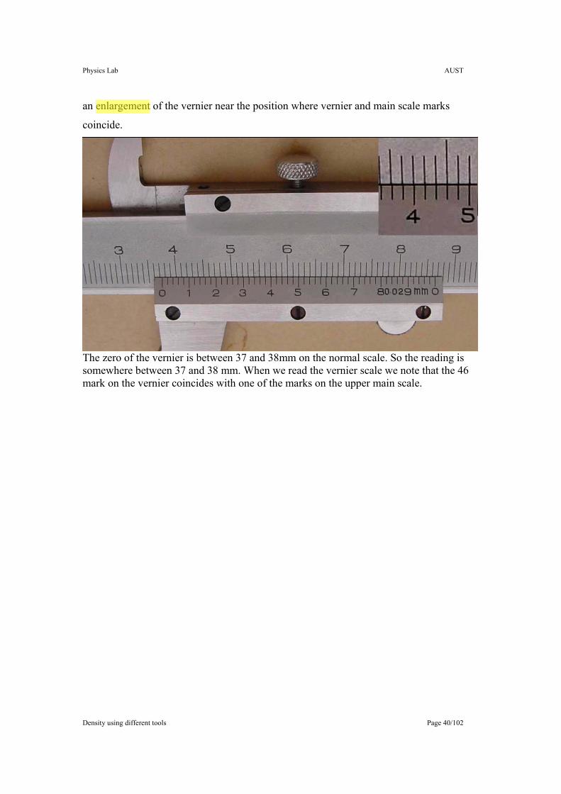
In is not unusual to find vernier scales with a nominal precision of 0.02 mm as
shown in the picture below. Note that the inset in the top right of the photograph shows
Physics Lab AUST
Density using different tools Page 40/102
an enlargement of the vernier near the position where vernier and main scale marks
coincide.
The zero of the vernier is between 37 and 38mm on the normal scale. So the reading is somewhere between 37 and 38 mm. When we read the vernier scale we note that the 46 mark on the vernier coincides with one of the marks on the upper main scale.
Physics Lab AUST
Density using different tools Page 41/102
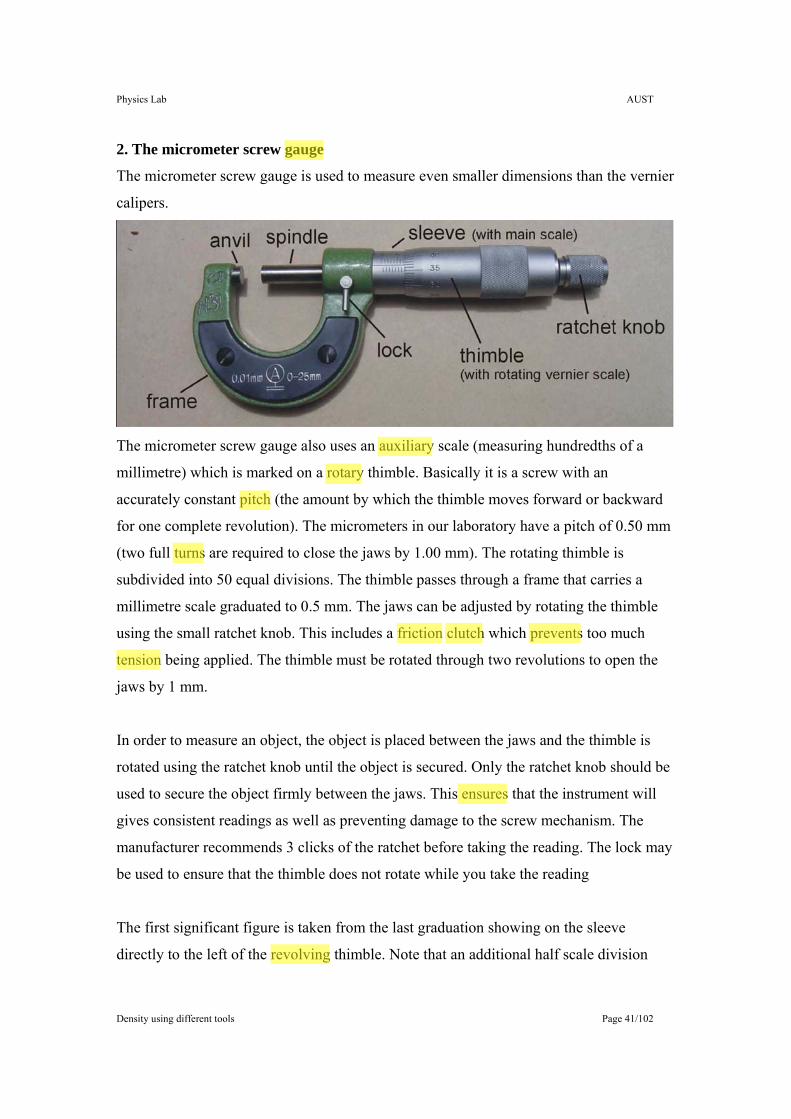
2. The micrometer screw gauge
The micrometer screw gauge is used to measure even smaller dimensions than the vernier
calipers.
The micrometer screw gauge also uses an auxiliary scale (measuring hundredths of a
millimetre) which is marked on a rotary thimble. Basically it is a screw with an
accurately constant pitch (the amount by which the thimble moves forward or backward
for one complete revolution). The micrometers in our laboratory have a pitch of 0.50 mm
(two full turns are required to close the jaws by 1.00 mm). The rotating thimble is
subdivided into 50 equal divisions. The thimble passes through a frame that carries a
millimetre scale graduated to 0.5 mm. The jaws can be adjusted by rotating the thimble
using the small ratchet knob. This includes a friction clutch which prevents too much
tension being applied. The thimble must be rotated through two revolutions to open the
jaws by 1 mm.
In order to measure an object, the object is placed between the jaws and the thimble is
rotated using the ratchet knob until the object is secured. Only the ratchet knob should be
used to secure the object firmly between the jaws. This ensures that the instrument will
gives consistent readings as well as preventing damage to the screw mechanism. The
manufacturer recommends 3 clicks of the ratchet before taking the reading. The lock may
be used to ensure that the thimble does not rotate while you take the reading
The first significant figure is taken from the last graduation showing on the sleeve
directly to the left of the revolving thimble. Note that an additional half scale division
Physics Lab AUST
Density using different tools Page 42/102
(0.5 mm) must be included if the mark below the main scale is visible between the
thimble and the main scale division on the sleeve. The remaining two significant figures
(hundredths of a millimetre) are taken directly from the thimble opposite the main scale.
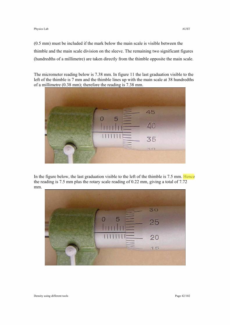
The micrometer reading below is 7.38 mm. In figure 11 the last graduation visible to the left of the thimble is 7 mm and the thimble lines up with the main scale at 38 hundredths of a millimetre (0.38 mm); therefore the reading is 7.38 mm.
In the figure below, the last graduation visible to the left of the thimble is 7.5 mm. Hence the reading is 7.5 mm plus the rotary scale reading of 0.22 mm, giving a total of 7.72 mm.

Physics Lab AUST
Density using different tools Page 43/102
Procedure:
To train on the internet about using these devices , please, work with these websites:
http://members.shaw.ca/ron.blond/Vern.APPLET/index.html
http://members.shaw.ca/ron.blond/Micrometer.APPLET/
After training, Follow these steps:
10. Pick metal piece (Cylindrical Piece like Dirham).
11. Get the diameter and thickness by ruler, vernier, and micrometer, be careful about
significant digits.
12. Get mass using digital Balance.
13. Get volume and density.
14. Tabulate your results.
Physics Lab AUST
Density using different tools Page 44/102
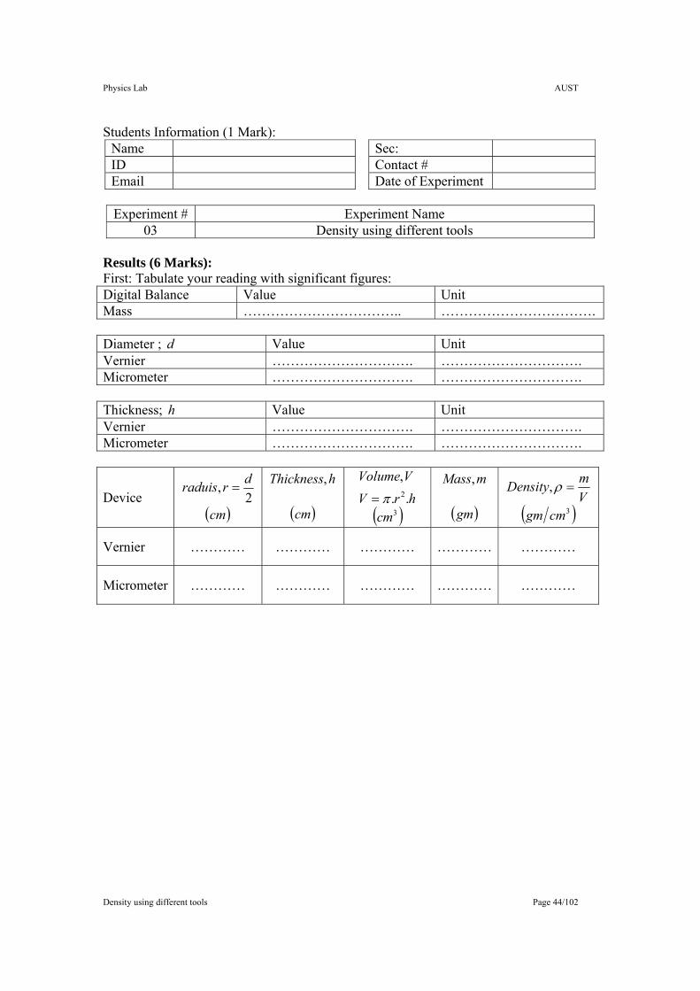
Students Information (1 Mark): Name Sec: ID Contact # Email Date of Experiment
Experiment # Experiment Name
03 Density using different tools Results (6 Marks): First: Tabulate your reading with significant figures: Digital Balance Value Unit Mass …………………………….. ……………………………. Diameter ; d Value Unit Vernier …………………………. …………………………. Micrometer …………………………. …………………………. Thickness; h Value Unit Vernier …………………………. …………………………. Micrometer …………………………. ………………………….
Device 2, drraduis =
( )cm
hThickness,
( )cm hrV
VVolume..
,2π=
( )3cm
mMass,
( )gm VmDensity =ρ,
( )3cmgm
Vernier ………… ………… ………… ………… …………
Micrometer ………… ………… ………… ………… …………
Physics Lab AUST
Density using different tools Page 45/102
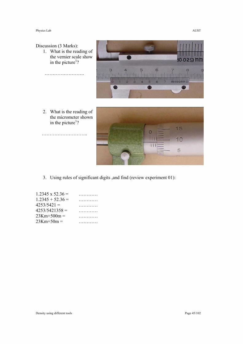
Discussion (3 Marks): 1. What is the reading of
the vernier scale show in the picture1?
…………………….
2. What is the reading of the micrometer shown in the picture1?
………………………..
3. Using rules of significant digits ,and find (review experiment 01): 1.2345 x 52.36 = ………… 1.2345 + 52.36 = ………… 4253/5421 = ………… 4253/5421358 = ………… 23Km+500m = ………… 23Km+50m = …………
Physics Lab AUST
Vectors (free body diagram) Page 46/102
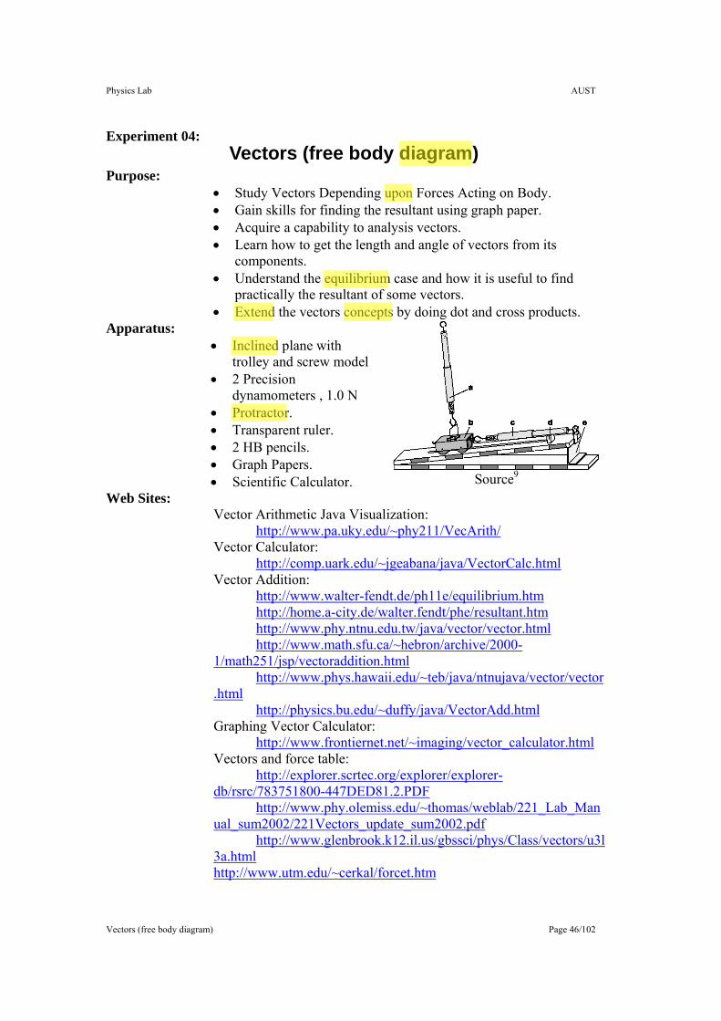
Experiment 04: Vectors (free body diagram)
Purpose: • Study Vectors Depending upon Forces Acting on Body. • Gain skills for finding the resultant using graph paper. • Acquire a capability to analysis vectors. • Learn how to get the length and angle of vectors from its
components. • Understand the equilibrium case and how it is useful to find
practically the resultant of some vectors. • Extend the vectors concepts by doing dot and cross products.
Apparatus: • Inclined plane with
trolley and screw model • 2 Precision
dynamometers , 1.0 N • Protractor. • Transparent ruler. • 2 HB pencils. • Graph Papers. • Scientific Calculator.
Source9
Web Sites: Vector Arithmetic Java Visualization:
http://www.pa.uky.edu/~phy211/VecArith/ Vector Calculator:
http://comp.uark.edu/~jgeabana/java/VectorCalc.html Vector Addition:
http://www.walter-fendt.de/ph11e/equilibrium.htm http://home.a-city.de/walter.fendt/phe/resultant.htm http://www.phy.ntnu.edu.tw/java/vector/vector.html http://www.math.sfu.ca/~hebron/archive/2000-
1/math251/jsp/vectoraddition.html http://www.phys.hawaii.edu/~teb/java/ntnujava/vector/vector
.html http://physics.bu.edu/~duffy/java/VectorAdd.html
Graphing Vector Calculator: http://www.frontiernet.net/~imaging/vector_calculator.html
Vectors and force table: http://explorer.scrtec.org/explorer/explorer-
db/rsrc/783751800-447DED81.2.PDF http://www.phy.olemiss.edu/~thomas/weblab/221_Lab_Man
ual_sum2002/221Vectors_update_sum2002.pdf http://www.glenbrook.k12.il.us/gbssci/phys/Class/vectors/u3l
3a.html http://www.utm.edu/~cerkal/forcet.htm
Physics Lab AUST
Vectors (free body diagram) Page 47/102
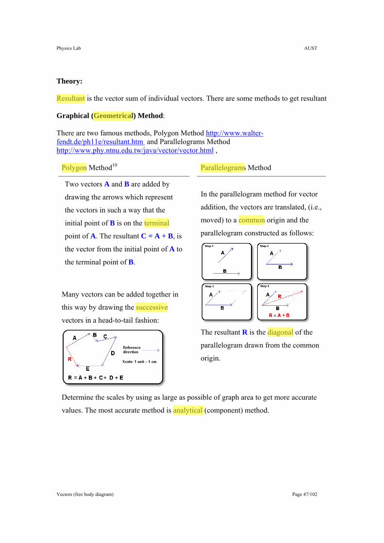
Theory: Resultant is the vector sum of individual vectors. There are some methods to get resultant Graphical (Geometrical) Method: There are two famous methods, Polygon Method http://www.walter-fendt.de/ph11e/resultant.htm and Parallelograms Method http://www.phy.ntnu.edu.tw/java/vector/vector.html ,
Polygon Method10 Parallelograms Method
Two vectors A and B are added by
drawing the arrows which represent
the vectors in such a way that the
initial point of B is on the terminal
point of A. The resultant C = A + B, is
the vector from the initial point of A to
the terminal point of B.
Many vectors can be added together in
this way by drawing the successive
vectors in a head-to-tail fashion:
In the parallelogram method for vector
addition, the vectors are translated, (i.e.,
moved) to a common origin and the
parallelogram constructed as follows:
The resultant R is the diagonal of the
parallelogram drawn from the common
origin.
Determine the scales by using as large as possible of graph area to get more accurate
values. The most accurate method is analytical (component) method.
Physics Lab AUST
Vectors (free body diagram) Page 48/102
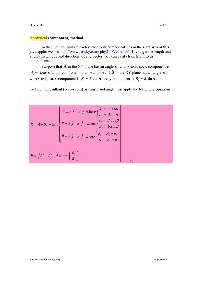
Analytical (component) method:
In this method, analyze each vector to its components, as in the right area of this java applet web sit http://www.pa.uky.edu/~phy211/VecArith/ . If you get the length and angle (magnitude and direction) of any vector, you can easily translate it to its components.
Suppose that Av
in the XY plane has an angle α with x-axis, so, x-component is αcos.AAx = and y-component is αsin.AAy = . If B
v in the XY plane has an angle β
with x-axis, so, x-component is βcos.BBx = and y-component is βsin.BBy = . To find the resultant (vector sum) as length and angle, just apply the following equations:
tan ,
where, ˆˆ
sin.cos.
where, ˆˆ
sin.cos.
where, ˆˆ
where,
22⎟⎟⎠
⎞⎜⎜⎝
⎛=+=
⎪⎪⎪⎪
⎩
⎪⎪⎪⎪
⎨
⎧
⎩⎨⎧
+=+=
+=
⎩⎨⎧
==
+=
⎩⎨⎧
==
+=
+=
−
x
yyx
yyy
xxxyx
y
xyx
y
xyx
RR
RRR
BARBAR
jRiRR
BBBB
jBiBB
AAAA
jAiAA
BAR
θ
ββαα
r
r
r
rrr
……(1)
Physics Lab AUST
Vectors (free body diagram) Page 49/102
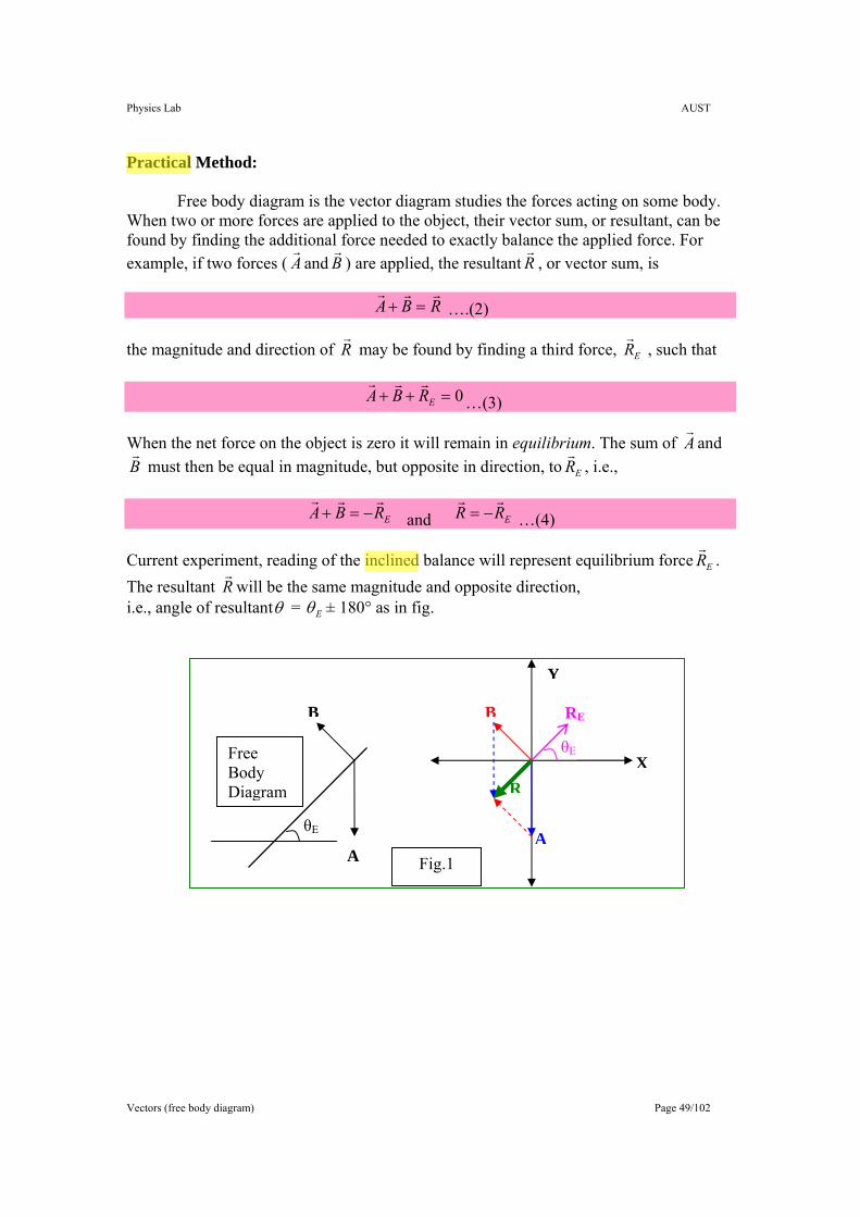
Practical Method:
Free body diagram is the vector diagram studies the forces acting on some body. When two or more forces are applied to the object, their vector sum, or resultant, can be found by finding the additional force needed to exactly balance the applied force. For example, if two forces ( A
rand B
r) are applied, the resultant R
r, or vector sum, is
RBArrr
=+ ….(2)
the magnitude and direction of Rr
may be found by finding a third force, ERr
, such that
0=++ ERBArrr
…(3)
When the net force on the object is zero it will remain in equilibrium. The sum of Ar
and Br
must then be equal in magnitude, but opposite in direction, to ERr
, i.e.,
ERBArrr
−=+ and ERRrr
−= …(4)
Current experiment, reading of the inclined balance will represent equilibrium force ERr
. The resultant R
rwill be the same magnitude and opposite direction,
i.e., angle of resultantθ = Eθ ± 180° as in fig.
θE
θE
RE
A
R
B
A
B
Y
X
Fig.1
Free Body Diagram
Physics Lab AUST
Vectors (free body diagram) Page 50/102
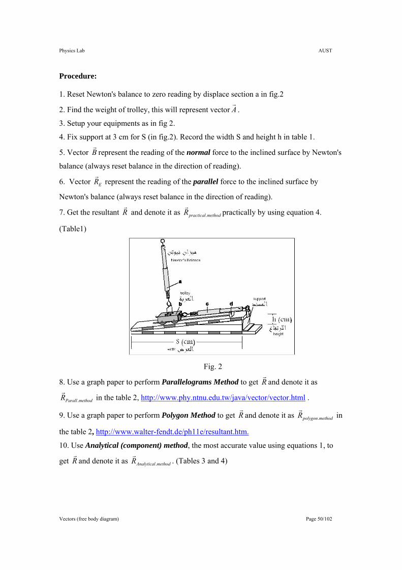
Procedure: 1. Reset Newton's balance to zero reading by displace section a in fig.2
2. Find the weight of trolley, this will represent vector Ar
.
3. Setup your equipments as in fig 2.
4. Fix support at 3 cm for S (in fig.2). Record the width S and height h in table 1.
5. Vector Br
represent the reading of the normal force to the inclined surface by Newton's
balance (always reset balance in the direction of reading).
6. Vector ERr
represent the reading of the parallel force to the inclined surface by
Newton's balance (always reset balance in the direction of reading).
7. Get the resultant Rr
and denote it as methodpracticalR .
rpractically by using equation 4.
(Table1)
Fig. 2
8. Use a graph paper to perform Parallelograms Method to get Rr
and denote it as
methodParallR .
r in the table 2, http://www.phy.ntnu.edu.tw/java/vector/vector.html .
9. Use a graph paper to perform Polygon Method to get Rr
and denote it as methodpolygonR .
r in
the table 2, http://www.walter-fendt.de/ph11e/resultant.htm.
10. Use Analytical (component) method, the most accurate value using equations 1, to
get Rr
and denote it as methodAnalyticalR .
r. (Tables 3 and 4)
Physics Lab AUST
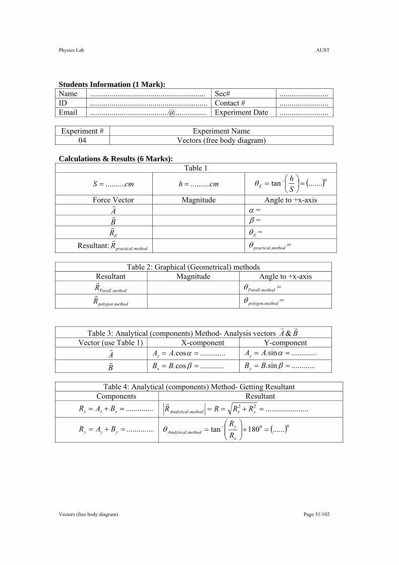
Vectors (free body diagram) Page 51/102
Students Information (1 Mark): Name ........................................................... Sec# ......................... ID ............................................................ Contact # ......................... Email ........................................@................ Experiment Date ......................... Experiment # Experiment Name
04 Vectors (free body diagram) Calculations & Results (6 Marks):
Table 1
cmS ..........= cmh ..........= ( )0.......tan =⎟⎠⎞
⎜⎝⎛= −
Sh
Eθ
Force Vector Magnitude Angle to +x-axis Ar
α = Br
β =
ERr
Eθ =
Resultant: methodpracticalR .
r methodpractical.θ =
Table 2: Graphical (Geometrical) methods
Resultant Magnitude Angle to +x-axis
methodParallR .
r methodParall .θ =
methodpolygonR .
r methodpolygon.θ =
Table 3: Analytical (components) Method- Analysis vectors Ar
& Br
Vector (use Table 1) X-component Y-component
Ar
.............cos. == αAAx .............sin. == αAAy
Br
............cos. == βBBx ............sin. == βBBy
Table 4: Analytical (components) Method- Getting Resultant Components Resultant
..............=+= xxx BAR ......................22. =+== yxmethodAnalytical RRRR
r
..............=+= yyy BAR ( )00. ......180tan =+⎟⎟
⎠
⎞⎜⎜⎝
⎛= −
x
ymethodAnalytical R
Rθ
Physics Lab AUST
Vectors (free body diagram) Page 52/102
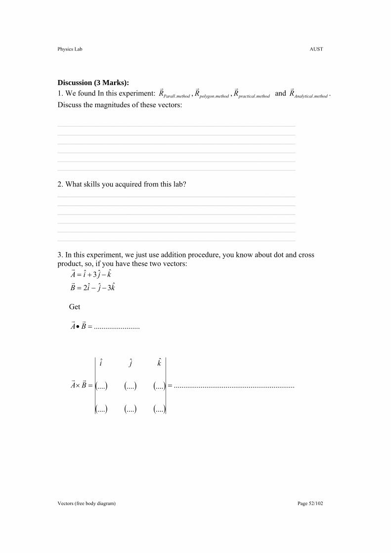
Discussion (3 Marks): 1. We found In this experiment: methodParallR .
r, methodpolygonR .
r, methodpracticalR .
r and methodAnalyticalR .
r.
Discuss the magnitudes of these vectors:
______________________________________________________________ ______________________________________________________________ ______________________________________________________________ ______________________________________________________________ ______________________________________________________________ ______________________________________________________________
2. What skills you acquired from this lab? ______________________________________________________________ ______________________________________________________________ ______________________________________________________________ ______________________________________________________________ ______________________________________________________________ ______________________________________________________________ 3. In this experiment, we just use addition procedure, you know about dot and cross product, so, if you have these two vectors:
kjiB
kjiAˆ3ˆˆ2
ˆˆ3ˆ
−−=
−+=r
r
Get
( ) ( ) ( )
( ) ( ) ( )
...............................................................
............
............
ˆˆˆ
........................
==×
=•
kji
BA
BA
rr
rr
Physics Lab AUST
Motion Along Straight line and Newton's laws Page 53/102
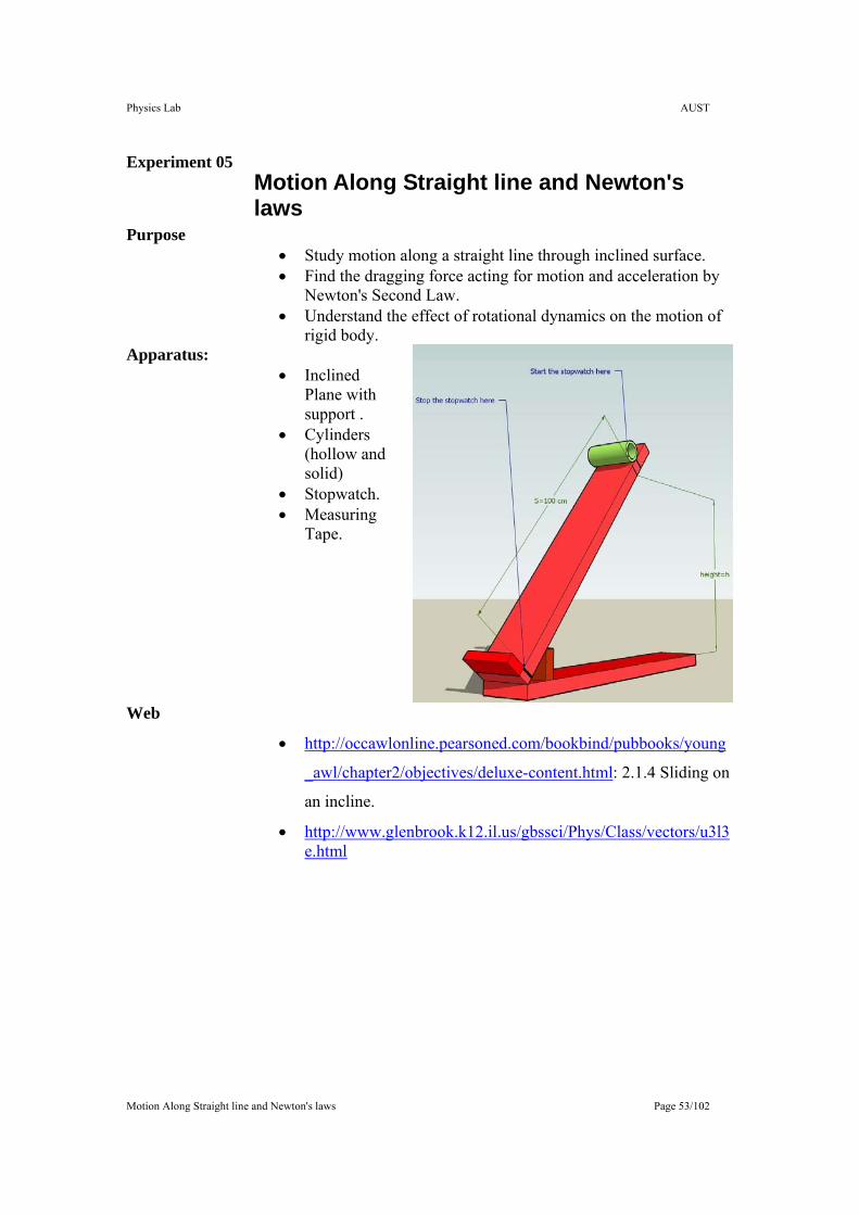
Motion Along Straight line and Newton's laws
Experiment 05
• Study motion along a straight line through inclined surface. • Find the dragging force acting for motion and acceleration by
Newton's Second Law. • Understand the effect of rotational dynamics on the motion of
rigid body.
Purpose
• Inclined
Plane with support .
• Cylinders (hollow and solid)
• Stopwatch. • Measuring
Tape.
Apparatus:
• http://occawlonline.pearsoned.com/bookbind/pubbooks/young
_awl/chapter2/objectives/deluxe-content.html: 2.1.4 Sliding on
an incline.
• http://www.glenbrook.k12.il.us/gbssci/Phys/Class/vectors/u3l3e.html
Web
Physics Lab AUST
Motion Along Straight line and Newton's laws Page 54/102
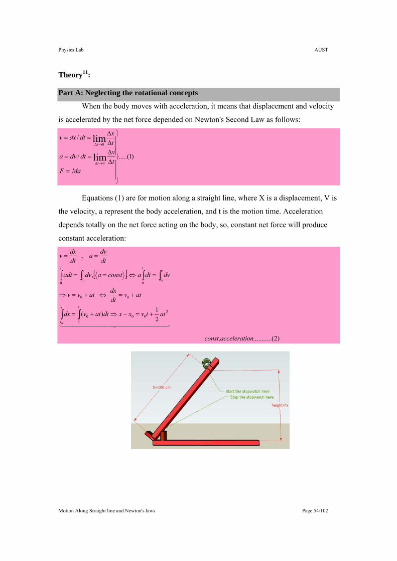
Theory11: Part A: Neglecting the rotational concepts
When the body moves with acceleration, it means that displacement and velocity
is accelerated by the net force depended on Newton's Second Law as follows:
)1.....(/
/
lim
lim
0
0
⎪⎪⎪
⎭
⎪⎪⎪
⎬
⎫
=∆∆
==
∆∆
==
→∆
→∆
MaFtvdtdva
txdtdxv
t
t
Equations (1) are for motion along a straight line, where X is a displacement, V is
the velocity, a represent the body acceleration, and t is the motion time. Acceleration
depends totally on the net force acting on the body, so, constant net force will produce
constant acceleration:
[ ]
)2.(...........
21)(
.,
,
200
00
00
00
0
00
onacceleraticonst
attvxxdtatvdx
atvdtdxatvv
dvdtaconstadvadt
dtdva
dtdxv
tx
x
v
v
tv
v
t
4444444 34444444 21
+=−⇒+=
+=⇔+=⇒
=⇔==
==
∫∫
∫∫∫∫
Physics Lab AUST
Motion Along Straight line and Newton's laws Page 55/102
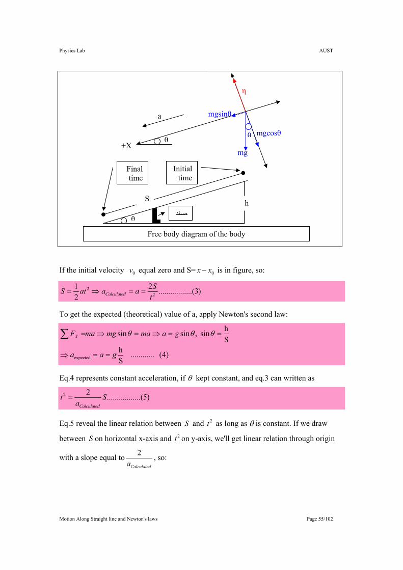
If the initial velocity 0v equal zero and S= 0xx − is in figure, so:
)3.......(..........221
22
tSaaatS Calculated ==⇒=
To get the expected (theoretical) value of a, apply Newton's second law:
)4( ............ Sh
Shsin ,sinsin
expected gaa
gamamgmaFX
==⇒
==⇒=⇒=∑ θθθ
Eq.4 represents constant acceleration, if θ kept constant, and eq.3 can written as
)5.......(..........22 Sa
tCalculated
=
Eq.5 reveal the linear relation between S and 2t as long as θ is constant. If we draw
between S on horizontal x-axis and 2t on y-axis, we'll get linear relation through origin
with a slope equal toCalculateda
2 , so:
η
θmgcosθ θ
mgsinθ a
X+ mg
θ
S hمسند
Free body diagram of the body
Initial time
Final time
Physics Lab AUST
Motion Along Straight line and Newton's laws Page 56/102
(6) ........ 2slope
aCalculated = . And,
...(7) %100%expected
expected ×−
=a
aaError Calculated
Part B: Considering rotational concepts into calculations.
As you see here, we have a rigid body rotates about its axis. We have to include
the rotational concepts to minimize the error above because some of the kinetic energy
will convert to rotational energy. That’s why expected acceleration is substantially
greater than calculated in part A.
Now, we are considering the rotational concepts, the kinetic energy K and
potential energyU :
22 .
21.
21 wIvMK CMCM += , MghU = where
o M : Mass of rigid body,
o CMv : Center of Mass velocity,
o ∑= 2iiCM rmI : Moment of inertia and 2cMRICM = for symmetric bodies of
radius R , c is numerical constant depends on the distribution of mass around axis
of rotation.
• Moment of inertia for hollow cylinder is 2MRICM = gave me 1=c for it.
• Moment of inertia for solid cylinder is 2
21 MRICM = gave me 5.0=c for it.
• Moment of inertia for solid sphere is 2
52 MRICM = gave me 4.0=c for it.
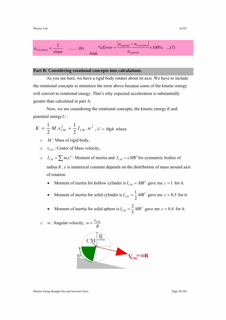
o w : Angular velocity, R
vw CM=
Physics Lab AUST
Motion Along Straight line and Newton's laws Page 57/102
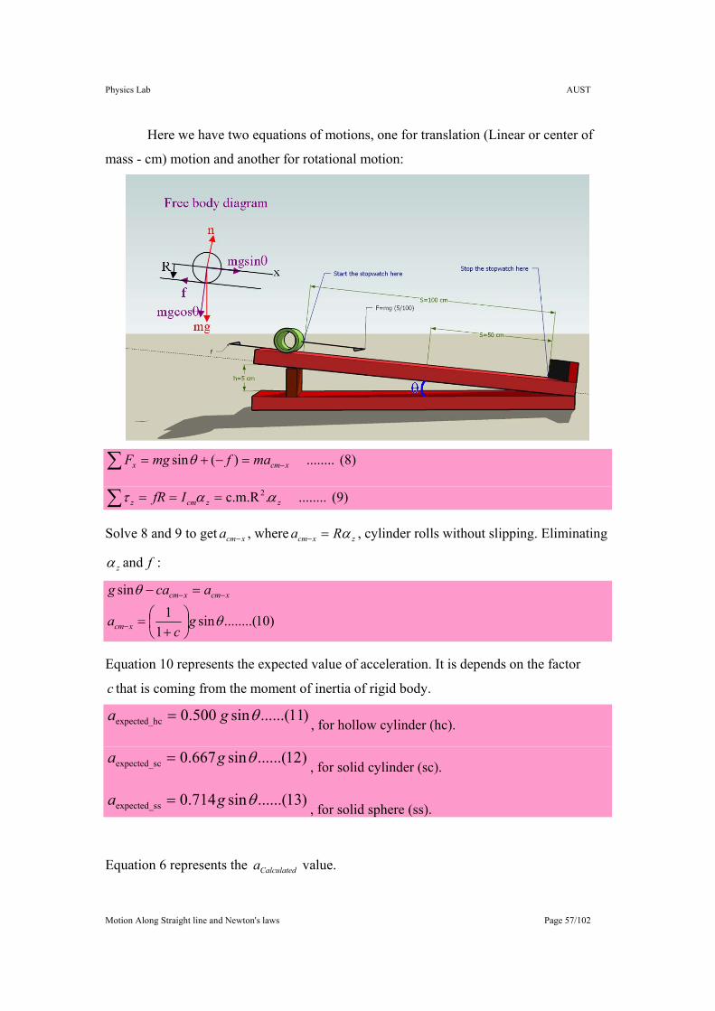
Here we have two equations of motions, one for translation (Linear or center of
mass - cm) motion and another for rotational motion:
(8) ........ )(sin xcmx mafmgF −=−+=∑ θ
(9) ........ .c.m.R2zzcmz IfR αατ ===∑
Solve 8 and 9 to get xcma − , where zxcm Ra α=− , cylinder rolls without slipping. Eliminating
zα and f :
)10........(sin1
1sin
θ
θ
gc
a
acag
xcm
xcmxcm
⎟⎠⎞
⎜⎝⎛+
=
=−
−
−−
Equation 10 represents the expected value of acceleration. It is depends on the factor
c that is coming from the moment of inertia of rigid body.
)11......(sin 500.0cexpected_h θga =, for hollow cylinder (hc).
)12......(sin667.0cexpected_s θga =, for solid cylinder (sc).
)13......(sin714.0sexpected_s θga =, for solid sphere (ss).
Equation 6 represents the Calculateda value.
Physics Lab AUST
Motion Along Straight line and Newton's laws Page 58/102
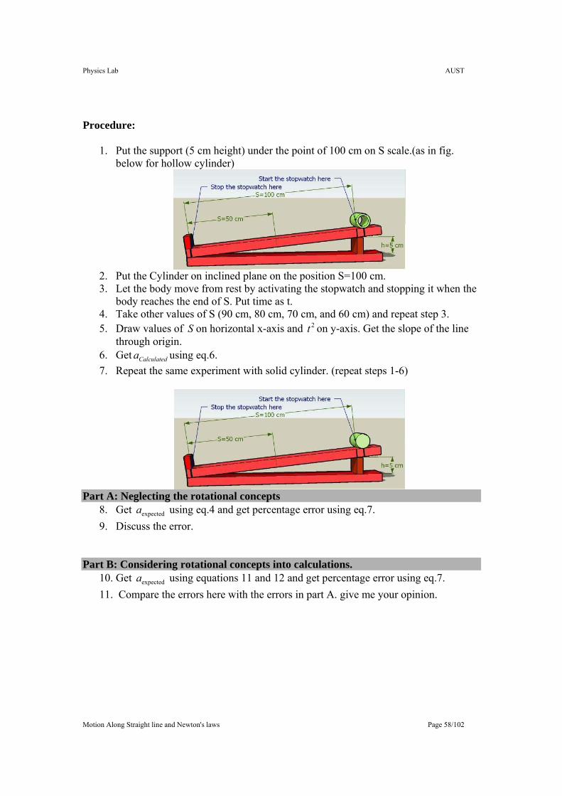
Procedure:
1. Put the support (5 cm height) under the point of 100 cm on S scale.(as in fig. below for hollow cylinder)
2. Put the Cylinder on inclined plane on the position S=100 cm. 3. Let the body move from rest by activating the stopwatch and stopping it when the
body reaches the end of S. Put time as t. 4. Take other values of S (90 cm, 80 cm, 70 cm, and 60 cm) and repeat step 3. 5. Draw values of S on horizontal x-axis and 2t on y-axis. Get the slope of the line
through origin. 6. Get Calculateda using eq.6. 7. Repeat the same experiment with solid cylinder. (repeat steps 1-6)
Part A: Neglecting the rotational concepts
8. Get expecteda using eq.4 and get percentage error using eq.7. 9. Discuss the error.
Part B: Considering rotational concepts into calculations.
10. Get expecteda using equations 11 and 12 and get percentage error using eq.7. 11. Compare the errors here with the errors in part A. give me your opinion.
Physics Lab AUST
Motion Along Straight line and Newton's laws Page 59/102
Student Details(1 Mark): Name ........................................................... Sec# ......................... ID ............................................................ Contact # ......................... Email ........................................@................ Experiment Date ......................... Experiment # Experiment Name
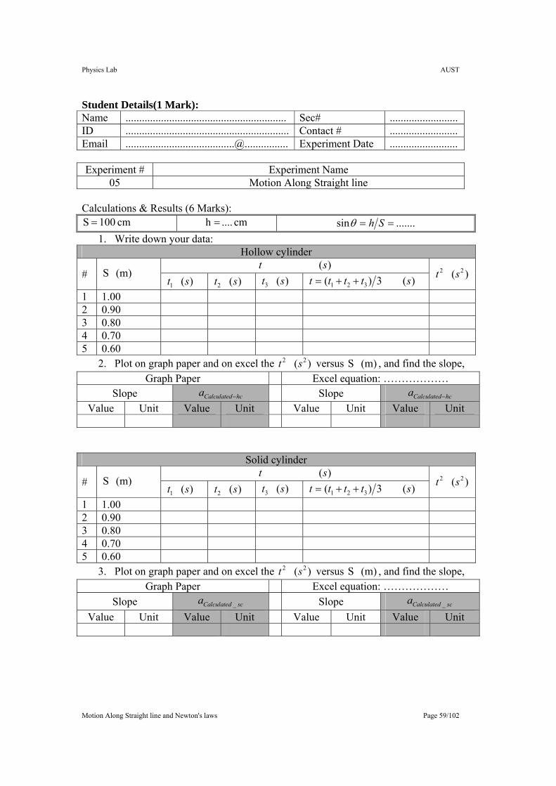
05 Motion Along Straight line Calculations & Results (6 Marks):
cm 100S = cm .... h = .......sin == Shθ 1. Write down your data:
Hollow cylinder )( st
# (m) S )( 1 st )( 2 st )( 3 st )( 3)( 321 stttt ++= )( 22 st
1 1.00 2 0.90 3 0.80 4 0.70 5 0.60
2. Plot on graph paper and on excel the )( 22 st versus (m) S , and find the slope, Graph Paper Excel equation: ………………
Slope hcCalculateda − Slope hcCalculateda − Value Unit Value Unit Value Unit Value Unit
Solid cylinder )( st
# (m) S )( 1 st )( 2 st )( 3 st )( 3)( 321 stttt ++= )( 22 st
1 1.00 2 0.90 3 0.80 4 0.70 5 0.60
3. Plot on graph paper and on excel the )( 22 st versus (m) S , and find the slope, Graph Paper Excel equation: ………………
Slope scCalculateda _ Slope scCalculateda _ Value Unit Value Unit Value Unit Value Unit
Physics Lab AUST
Motion Along Straight line and Newton's laws Page 60/102
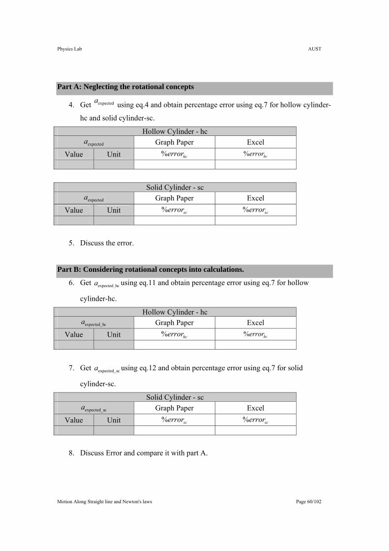
Part A: Neglecting the rotational concepts
4. Get expecteda using eq.4 and obtain percentage error using eq.7 for hollow cylinder-
hc and solid cylinder-sc.
Hollow Cylinder - hc expecteda Graph Paper Excel
Value Unit hcerror% hcerror%
Solid Cylinder - sc expecteda Graph Paper Excel
Value Unit scerror% scerror%
5. Discuss the error.
Part B: Considering rotational concepts into calculations.
6. Get cexpected_ha using eq.11 and obtain percentage error using eq.7 for hollow
cylinder-hc.
Hollow Cylinder - hc cexpected_ha Graph Paper Excel
Value Unit hcerror% hcerror%
7. Get cexpected_sa using eq.12 and obtain percentage error using eq.7 for solid
cylinder-sc.
Solid Cylinder - sc cexpected_sa Graph Paper Excel
Value Unit scerror% scerror%
8. Discuss Error and compare it with part A.
Physics Lab AUST
Motion Along Straight line and Newton's laws Page 61/102
Discussion (3 Marks):
1. Discuss the percentage errors in parts A and B:
______________________________________________________________
______________________________________________________________
______________________________________________________________
2. If S=10.0 m and angle of inclined surface is 30°,
• Get the acceleration for:
slipping object (no friction): _______________
Solid sphere without slipping: _______________
slipping Solid cylinder (no rotation): _______________
• Is there any change to the acceleration if S=20.0 m? Why?
______________________________________________________________
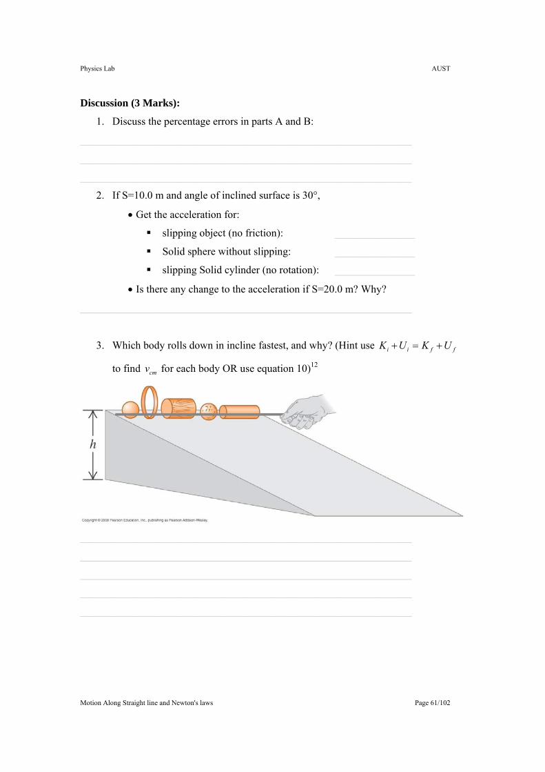
3. Which body rolls down in incline fastest, and why? (Hint use ffii UKUK +=+
to find cmv for each body OR use equation 10)12
______________________________________________________________
______________________________________________________________
______________________________________________________________
______________________________________________________________
______________________________________________________________
Physics Lab AUST
Friction Page 62/102
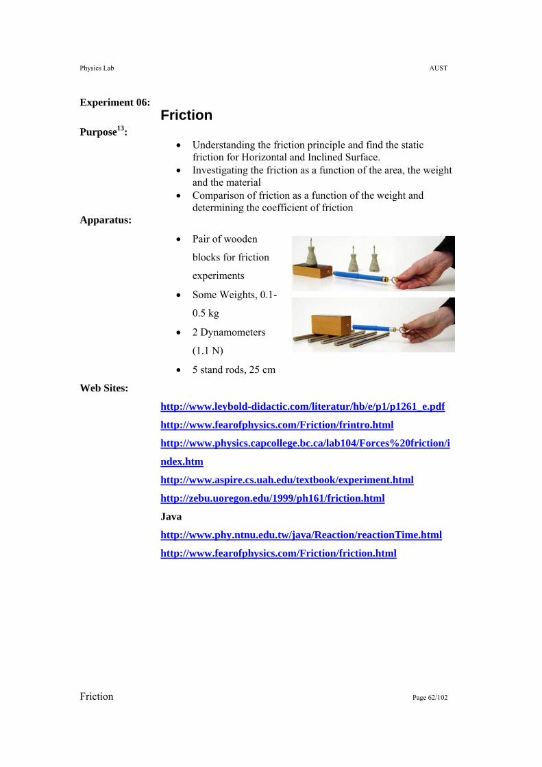
Experiment 06: Friction
Purpose13: • Understanding the friction principle and find the static
friction for Horizontal and Inclined Surface. • Investigating the friction as a function of the area, the weight
and the material • Comparison of friction as a function of the weight and
determining the coefficient of friction Apparatus:
• Pair of wooden
blocks for friction
experiments
• Some Weights, 0.1-
0.5 kg
• 2 Dynamometers
(1.1 N)
• 5 stand rods, 25 cm
Web Sites:
http://www.leybold-didactic.com/literatur/hb/e/p1/p1261_e.pdf
http://www.fearofphysics.com/Friction/frintro.html
http://www.physics.capcollege.bc.ca/lab104/Forces%20friction/i
ndex.htm
http://www.aspire.cs.uah.edu/textbook/experiment.html
http://zebu.uoregon.edu/1999/ph161/friction.html
Java
http://www.phy.ntnu.edu.tw/java/Reaction/reactionTime.html
http://www.fearofphysics.com/Friction/friction.html
Physics Lab AUST
Friction Page 63/102
Theory14:
Frictional Forces: We have seen several problems where a body rests or slides
on a surface that exerts forces on the body. Whenever two bodies interact by direct
contact (touching) of their surfaces, we describe the interaction in terms of contact forces.
The normal force is one example of a contact force: we’ll look in detail at another contact
force, the force of friction.
Kinetic and Static Friction When you try to slide a heavy box of books across
the floor, the box doesn’t move at all unless you push with a certain minimum force.
Then the box starts moving, and you can usually keep it moving with less force than you
needed to get it started. If you take some of the books out, you need less force than before
to get it started or keep it moving. What general statements can we make about this
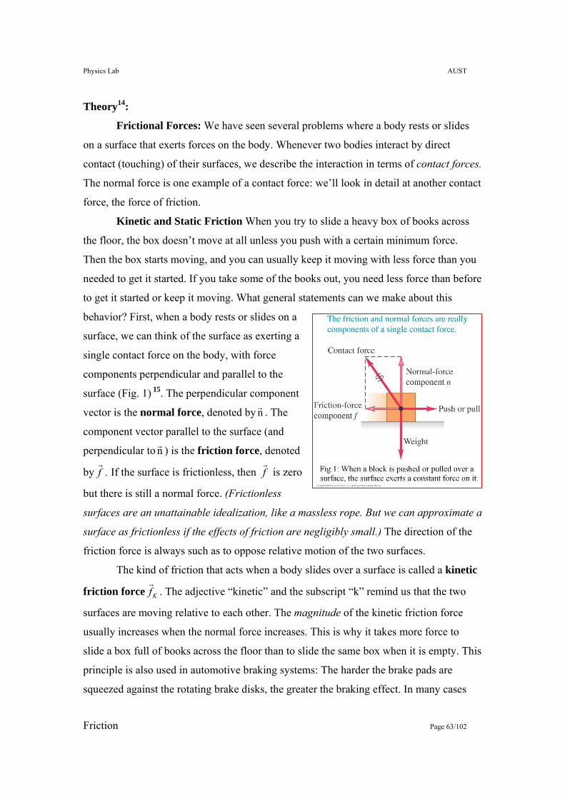
behavior? First, when a body rests or slides on a
surface, we can think of the surface as exerting a
single contact force on the body, with force
components perpendicular and parallel to the
surface (Fig. 1) 15. The perpendicular component
vector is the normal force, denoted by nr . The
component vector parallel to the surface (and
perpendicular to nr ) is the friction force, denoted
by fr
. If the surface is frictionless, then fr
is zero
but there is still a normal force. (Frictionless
surfaces are an unattainable idealization, like a massless rope. But we can approximate a
surface as frictionless if the effects of friction are negligibly small.) The direction of the
friction force is always such as to oppose relative motion of the two surfaces.
The kind of friction that acts when a body slides over a surface is called a kinetic
friction force Kfr
. The adjective “kinetic” and the subscript “k” remind us that the two
surfaces are moving relative to each other. The magnitude of the kinetic friction force
usually increases when the normal force increases. This is why it takes more force to
slide a box full of books across the floor than to slide the same box when it is empty. This
principle is also used in automotive braking systems: The harder the brake pads are
squeezed against the rotating brake disks, the greater the braking effect. In many cases
Physics Lab AUST
Friction Page 64/102
the magnitude of the kinetic friction force Kfr
is found experimentally to be
approximately proportional to the magnitude n of the normal force. In such cases we
represent the relationship by the equation
force)friction kinetic of (Magnitude nf KK µ= (1) where Kµ (pronounced “mu-sub-k”) is a constant called the coefficient of kinetic
friction. The more slippery the surface, the smaller the coefficient of friction. Because it
is a quotient of two force magnitudes, Kµ is a pure number, without units.
CAUTION Friction and normal forces are always perpendicular Remember that Eq. (1) is not a vector equation because Kfr
and n are always perpendicular. Rather it is a scalar relationship between the magnitudes of the two forces.
Friction forces may also act when there is no relative motion. If you try to slide a
box across the floor, the box may not move at all because the floor exerts an equal and
opposite friction force on the box. This is called a static friction force Sf . In Fig.216a, the
box is at rest, in equilibrium, under the action of its weight wr and the upward normal
force nr . The normal force is equal in magnitude to the weight ( wn = ) and is exerted on
the box by the floor. Now we tie a rope to the box (Fig.2b) and gradually increase the
Physics Lab AUST
Friction Page 65/102
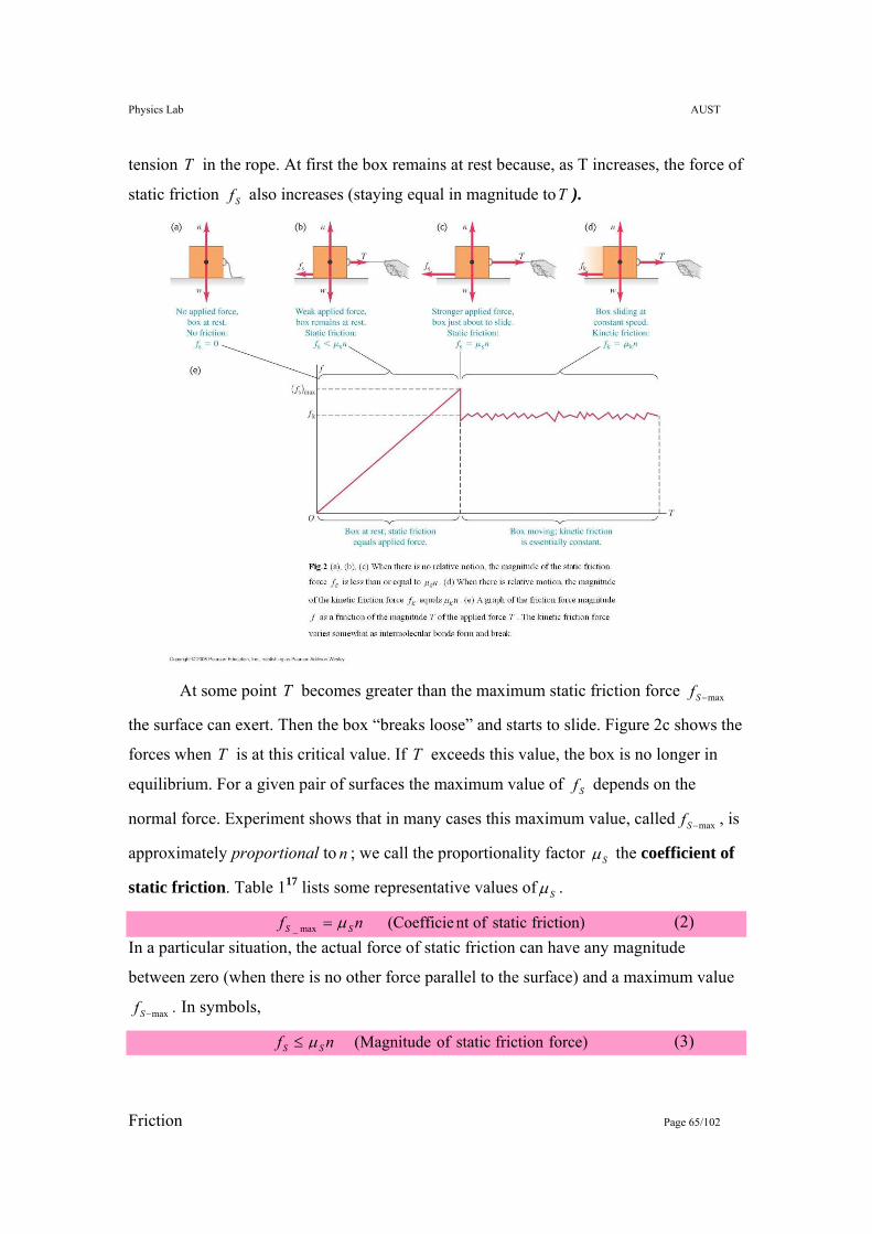
tension T in the rope. At first the box remains at rest because, as T increases, the force of
static friction Sf also increases (staying equal in magnitude toT ).
At some point T becomes greater than the maximum static friction force max−Sf
the surface can exert. Then the box “breaks loose” and starts to slide. Figure 2c shows the
forces when T is at this critical value. If T exceeds this value, the box is no longer in
equilibrium. For a given pair of surfaces the maximum value of Sf depends on the
normal force. Experiment shows that in many cases this maximum value, called max−Sf , is
approximately proportional to n ; we call the proportionality factor Sµ the coefficient of
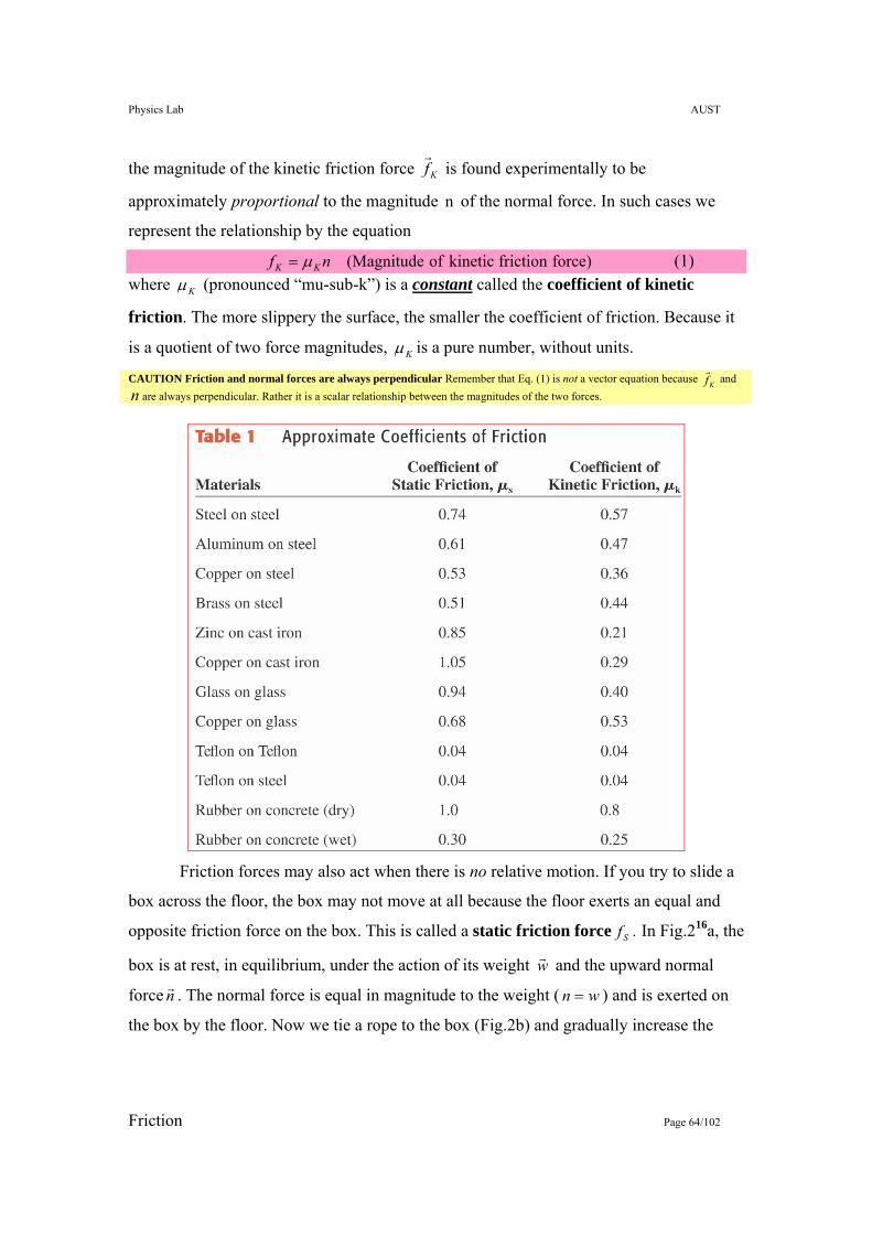
static friction. Table 117 lists some representative values of Sµ .
friction) static ofnt (Coefficie max_ nf SS µ= (2) In a particular situation, the actual force of static friction can have any magnitude
between zero (when there is no other force parallel to the surface) and a maximum value
max−Sf . In symbols,
force)friction static of (Magnitude nf SS µ≤ (3)
Physics Lab AUST
Friction Page 66/102
Like Eq. (1), this is a relationship between magnitudes, not a vector relationship. The
equality sign holds only when the applied force T has reached the critical value at which
motion is about to start (Fig.2c). When T is less than this value (Fig.2b), the inequality
sign holds. In that case we have to use the equilibrium conditions (∑ = 0Fr
) to find Sf .
If there is no applied force ( 0=T ) as in Fig.2a, then there is no static friction force either
( 0=Sf ).
As soon as the box starts to slide (Fig.2d), the friction force usually decreases; it’s
easier to keep the box moving than to start it moving. Hence the coefficient of kinetic
friction is usually less than the coefficient of static friction for any given pair of surfaces,
as Table 1 shows. If we start with no applied force ( 0=T ) and gradually increase the
force, the friction force varies somewhat, as shown in Fig.2e.
Rolling Friction: It’s a lot easier to move a loaded filing cabinet across a
horizontal floor using a cart with wheels than to slide it. How much easier? We can
define a coefficient of rolling friction rµ , which is the horizontal force needed for
constant speed on a flat surface divided by the upward normal force exerted by the
surface. Transportation engineers call rµ the tractive resistance. Typical values of rµ
are 0.002 to 0.003 for steel wheels on steel rails and 0.01 to 0.02 for rubber tires on
concrete. These values show one reason railroad trains are generally much more fuel
efficient than highway trucks.
force)friction rolling of (Magnitude nf rr µ= (4)
This experiment verifies that the static friction force and the kinetic friction force
are independent of the size of the contact surface and proportional to the normal force.
The coefficients of friction depend on the material of the contact surfaces. As the static
friction force is always greater than the kinetic friction force, we can always say
kS µµ > (5) To distinguish between Kinetic and rolling friction, the friction block is placed on
top of multiple stand rods laid parallel to each other. The rolling friction force
Physics Lab AUST
Friction Page 67/102
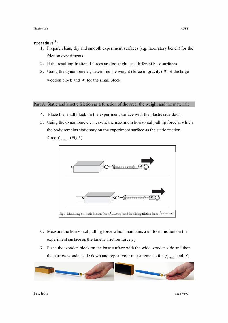
Procedure18: 1. Prepare clean, dry and smooth experiment surfaces (e.g. laboratory bench) for the
friction experiments.
2. If the resulting frictional forces are too slight, use different base surfaces.
3. Using the dynamometer, determine the weight (force of gravity) 1W of the large
wooden block and 2W for the small block.
Part A. Static and kinetic friction as a function of the area, the weight and the material:
4. Place the small block on the experiment surface with the plastic side down.
5. Using the dynamometer, measure the maximum horizontal pulling force at which
the body remains stationary on the experiment surface as the static friction
force max−Sf . (Fig.3)
6. Measure the horizontal pulling force which maintains a uniform motion on the
experiment surface as the kinetic friction force Kf .
7. Place the wooden block on the base surface with the wide wooden side and then
the narrow wooden side down and repeat your measurements for max−Sf and Kf .
Physics Lab AUST
Friction Page 68/102
8. Repeat the measurements with the large block for friction experiments.
9. Repeat the measurement on other surfaces as desired.
10. Tabulate your results in Table A and answer the questions related to the obtained
data.
Part B. Static and kinetic friction as a function of the force of gravity:
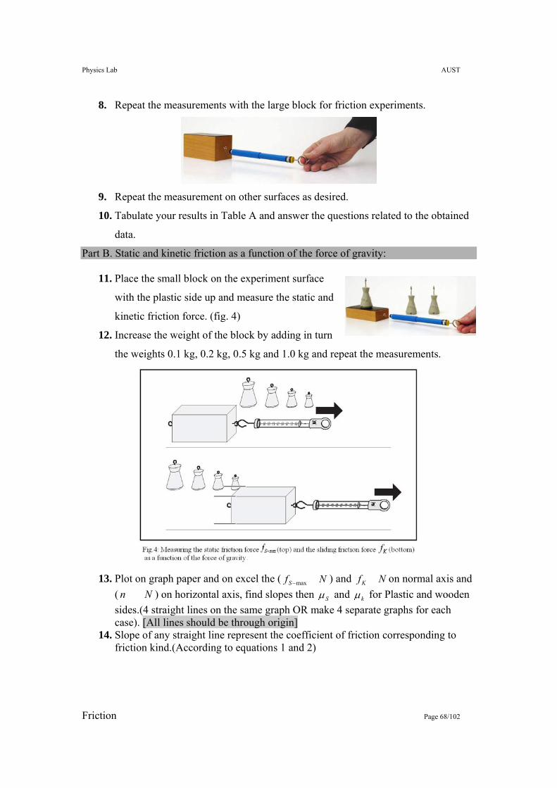
11. Place the small block on the experiment surface
with the plastic side up and measure the static and
kinetic friction force. (fig. 4)
12. Increase the weight of the block by adding in turn
the weights 0.1 kg, 0.2 kg, 0.5 kg and 1.0 kg and repeat the measurements.
13. Plot on graph paper and on excel the ( NfS max− ) and NfK on normal axis and
( Nn ) on horizontal axis, find slopes then Sµ and kµ for Plastic and wooden sides.(4 straight lines on the same graph OR make 4 separate graphs for each case). [All lines should be through origin]
14. Slope of any straight line represent the coefficient of friction corresponding to friction kind.(According to equations 1 and 2)
Physics Lab AUST
Friction Page 69/102
Part C. Rolling and kinetic friction as a function of the area, the weight and the material:
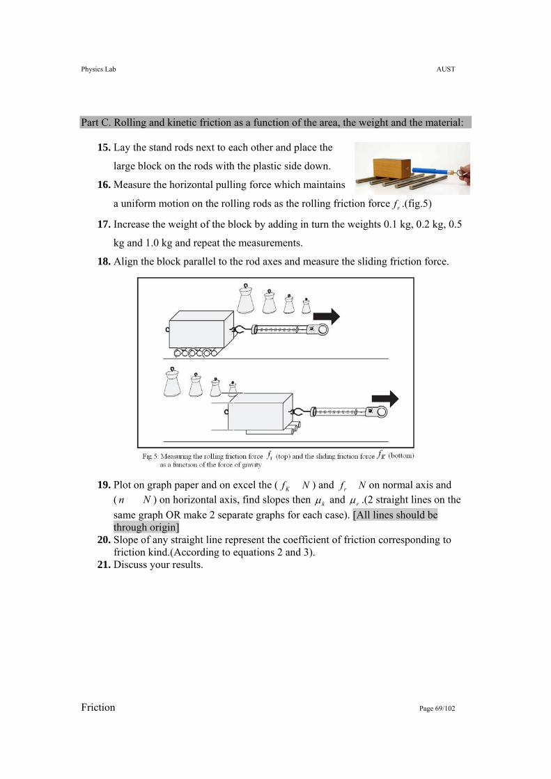
15. Lay the stand rods next to each other and place the
large block on the rods with the plastic side down.
16. Measure the horizontal pulling force which maintains
a uniform motion on the rolling rods as the rolling friction force rf .(fig.5)
17. Increase the weight of the block by adding in turn the weights 0.1 kg, 0.2 kg, 0.5
kg and 1.0 kg and repeat the measurements.
18. Align the block parallel to the rod axes and measure the sliding friction force.
19. Plot on graph paper and on excel the ( NfK ) and Nfr on normal axis and
( Nn ) on horizontal axis, find slopes then kµ and rµ .(2 straight lines on the same graph OR make 2 separate graphs for each case). [All lines should be through origin]
20. Slope of any straight line represent the coefficient of friction corresponding to friction kind.(According to equations 2 and 3).
21. Discuss your results.
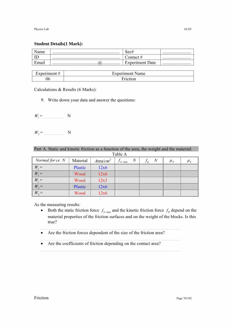
Physics Lab AUST
Friction Page 70/102
Student Details(1 Mark):
Name ........................................................... Sec# ......................... ID ............................................................ Contact # ......................... Email ........................................@................ Experiment Date ......................... Experiment # Experiment Name
06 Friction Calculations & Results (6 Marks):
9. Write down your data and answer the questions:
1W = _________ N
2W = _________ N
Part A. Static and kinetic friction as a function of the area, the weight and the material: Table A
NceNormal for Material 2rea/cmA NfS max− NfK Sµ kµ
1W = Plastic 12x6
1W = Wood 12x6
1W = Wood 12x3
2W = Plastic 12x6
2W = Wood 12x6 As the measuring results:
• Both the static friction force max−Sf and the kinetic friction force Kf depend on the material properties of the friction surfaces and on the weight of the blocks. Is this true?
______________________________________________________________ • Are the friction forces dependent of the size of the friction area?
______________________________________________________________ • Are the coefficients of friction depending on the contact area?
______________________________________________________________
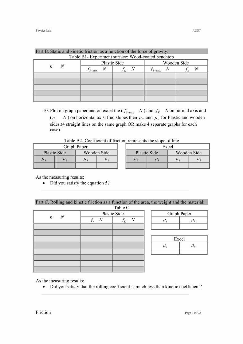
Physics Lab AUST
Friction Page 71/102
Part B. Static and kinetic friction as a function of the force of gravity:
Table B1- Experiment surface: Wood-coated benchtop Plastic Side Wooden Side
Nn NfS max− NfK NfS max− NfK
10. Plot on graph paper and on excel the ( NfS max− ) and NfK on normal axis and ( Nn ) on horizontal axis, find slopes then Sµ and kµ for Plastic and wooden sides.(4 straight lines on the same graph OR make 4 separate graphs for each case).
Table B2- Coefficient of friction represents the slope of line Graph Paper Excel
Plastic Side Wooden Side Plastic Side Wooden Side Sµ kµ Sµ kµ Sµ kµ Sµ kµ
As the measuring results:
• Did you satisfy the equation 5? ______________________________________________________________
Part C. Rolling and kinetic friction as a function of the area, the weight and the material: Table C
Plastic Side Graph Paper Nn Nfr NfK rµ kµ
Excel rµ kµ
As the measuring results:
• Did you satisfy that the rolling coefficient is much less than kinetic coefficient? ______________________________________________________________
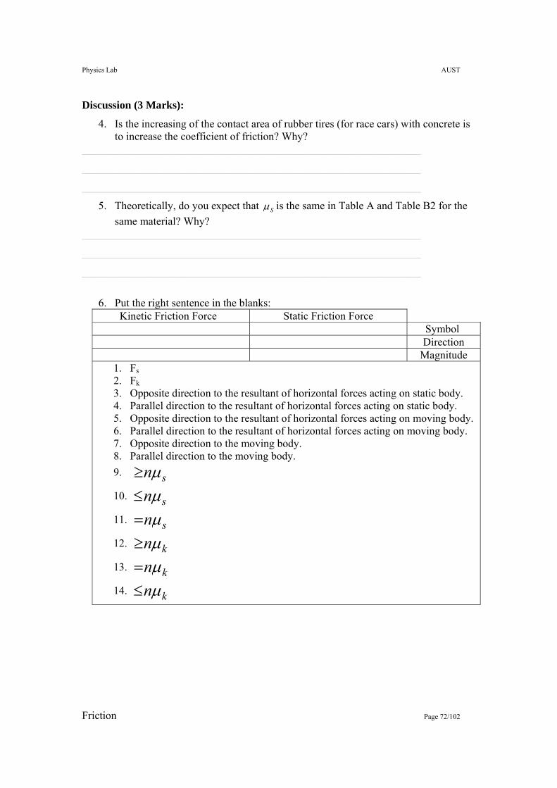
Physics Lab AUST
Friction Page 72/102
Discussion (3 Marks):
4. Is the increasing of the contact area of rubber tires (for race cars) with concrete is to increase the coefficient of friction? Why?
______________________________________________________________
______________________________________________________________
______________________________________________________________
5. Theoretically, do you expect that Sµ is the same in Table A and Table B2 for the same material? Why?
______________________________________________________________
______________________________________________________________
______________________________________________________________
6. Put the right sentence in the blanks:
Static Friction Force Kinetic Friction Force Symbol Direction
Magnitude 1. Fs 2. Fk 3. Opposite direction to the resultant of horizontal forces acting on static body. 4. Parallel direction to the resultant of horizontal forces acting on static body. 5. Opposite direction to the resultant of horizontal forces acting on moving body. 6. Parallel direction to the resultant of horizontal forces acting on moving body. 7. Opposite direction to the moving body. 8. Parallel direction to the moving body. 9. snµ≥
10. snµ≤
11. snµ=
12. knµ≥
13. knµ=
14. knµ≤
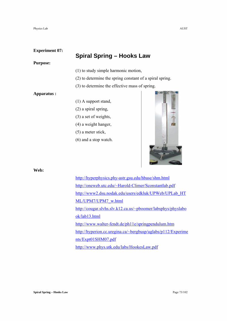
Physics Lab AUST
Spiral Spring – Hooks Law Page 73/102
Experiment 07: Spiral Spring – Hooks Law
Purpose:
(1) to study simple harmonic motion,
(2) to determine the spring constant of a spiral spring.
(3) to determine the effective mass of spring.
Apparatus :
(1) A support stand,
(2) a spiral spring,
(3) a set of weights,
(4) a weight hanger,
(5) a meter stick,
(6) and a stop watch.
Web:
http://hyperphysics.phy-astr.gsu.edu/hbase/shm.html
http://oneweb.utc.edu/~Harold-Climer/Sconstantlab.pdf
http://www2.dsu.nodak.edu/users/edkluk/UPWeb/UPLab_HT
ML/UPM7/UPM7_w.html
http://cougar.slvhs.slv.k12.ca.us/~pboomer/labsphys/physlabo
ok/lab13.html
http://www.walter-fendt.de/ph11e/springpendulum.htm
http://hyperion.cc.uregina.ca/~bergbusp/uglabs/p112/Experime
nts/Expt01SHM07.pdf
http://www.phys.utk.edu/labs/HookesLaw.pdf
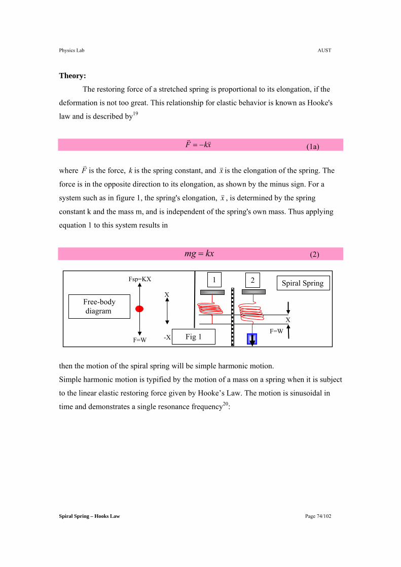
Physics Lab AUST
Spiral Spring – Hooks Law Page 74/102
Theory:
The restoring force of a stretched spring is proportional to its elongation, if the
deformation is not too great. This relationship for elastic behavior is known as Hooke's
law and is described by19
xkF vv−= (1a)
where Fv
is the force, k is the spring constant, and xv is the elongation of the spring. The
force is in the opposite direction to its elongation, as shown by the minus sign. For a
system such as in figure 1, the spring's elongation, xv , is determined by the spring
constant k and the mass m, and is independent of the spring's own mass. Thus applying
equation 1 to this system results in
kxmg = (2)
then the motion of the spiral spring will be simple harmonic motion.
Simple harmonic motion is typified by the motion of a mass on a spring when it is subject
to the linear elastic restoring force given by Hooke’s Law. The motion is sinusoidal in
time and demonstrates a single resonance frequency20:
X
Fig 1 F=W
1 2 Spiral Spring
F=W
Fsp=KX
X
-X
Free-body diagram
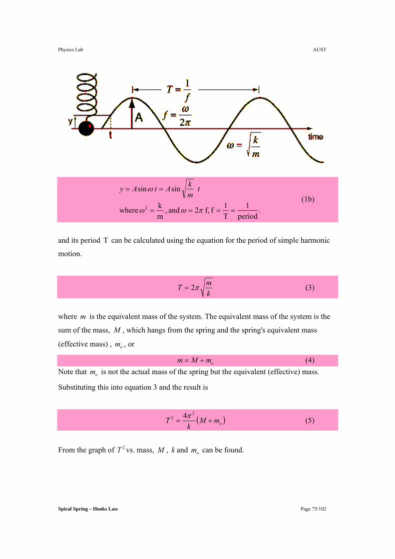
Physics Lab AUST
Spiral Spring – Hooks Law Page 75/102
.
period1
T1f f, 2 and ,
mk where
sin sin
2 ====
==
πωω
ω tmkAtAy
(1b)
and its period T can be calculated using the equation for the period of simple harmonic
motion.
kmT π2= (3)
where m is the equivalent mass of the system. The equivalent mass of the system is the
sum of the mass, M , which hangs from the spring and the spring's equivalent mass
(effective mass) , om , or
omMm += (4) Note that om is not the actual mass of the spring but the equivalent (effective) mass.
Substituting this into equation 3 and the result is
( )omMk
T +=2
2 4π (5)
From the graph of 2T vs. mass, M , k and om can be found.
Physics Lab AUST
Spiral Spring – Hooks Law Page 76/102
Procedure21:
1. Hang a 0.100 kg mass to the spiral spring, start the oscillation in a vertical
direction, and measure the time required for twenty complete oscillations. The
time for twenty oscillations should be repeated at least 3 times. [The small
amplitude is required in the oscillation. (2 or 3 cm will provide better result.)]
2. Calculate T, the system's period of oscillation.
3. Repeat step 2 for the masses 0.002 kg, 0.300 kg, 0.400 kg and 0.500 kg.
4. On Graph paper: Plot a graph of 2T vs. mass, M , and determine the spring
constant k from the relationship of slopek /4 2π= of this line.
5. On Graph paper: Determine om the equivalent (effective) mass of the spring by
extending the line down to cross the x-axis and figure the intercept on the x-axis.
6. On Excel: Graph the period T as a function of mass, M , using the chart feature
of Excel. The mass is the independent variable and should be plotted on the
horizontal axis or abscissa (x axis). The period is the dependent variable and
should be plotted on the vertical axis or ordinate (y axis).
7. On Excel: Use the trendline feature to draw a smooth curve that best fits your
data. To do this, from the main menu, choose Chart and then Add Trendline . . .
from the dropdown menu. This will bring up a Add Trendline dialog window.
From the Trend tab, choose Power from the Trend/Regression type selections.
Then click on the Options tab and select Display equations on chart and Display
R-squared value on chart options.
8. Examine the power function equation that is associated with the trendline. Does it
suggest the relationship between period and mass given by Equation (3)?
9. Examine your graph and notice that the change in the period per unit mass, the
slope of the curve, decreases as the mass increases. This indicates that the period
increases with the length at a rate less than a linear rate. The theory and Equation
(3) predict that the period depends on the square root of the mass. A graph of 2T versus M should result in a straight line.
10. Square the values of the period measured for each mass and record your results in
the table.
Physics Lab AUST
Spiral Spring – Hooks Law Page 77/102
11. On Excel: Use the chart feature again to graph the period squared, T2, as a
function of the mass. The period squared is the dependent variable and should be
plotted on the y axis. The mass is the independent variable and should be plotted
on the x axis.
12. Examine your graph of 2T versus M and check to see if there is a linear
relationship between 2T and M so that the data points lie along a line.
13. On Excel: Use the trendline feature to perform a linear regression to find a
straight line that best fits your data points. This time from the Add Trendline
dialog window. Choose Linear from the Trend/Regression type selections. Click
on the Options tab and once again select the Display equations on chart and
Display R-squared value on chart options. This should draw a straight line (not
through origin) that best fits the data and should display the equation for this
straight line.
14. On Excel: Equation (5) is of the form baxy += where 2Ty = and ka /4 2π= ,
oamb = , Mx = . A graph of 2T versus M should therefore result in a straight line
whose slope, a, is equal to k/4 2π . From the equation for the trendline, record the
value for the slope, a, the interception, b. From the equation ka /4 2π= find k , the
spring constant, and from the equation oamb = find om , the spring equivalent
(effective) mass.
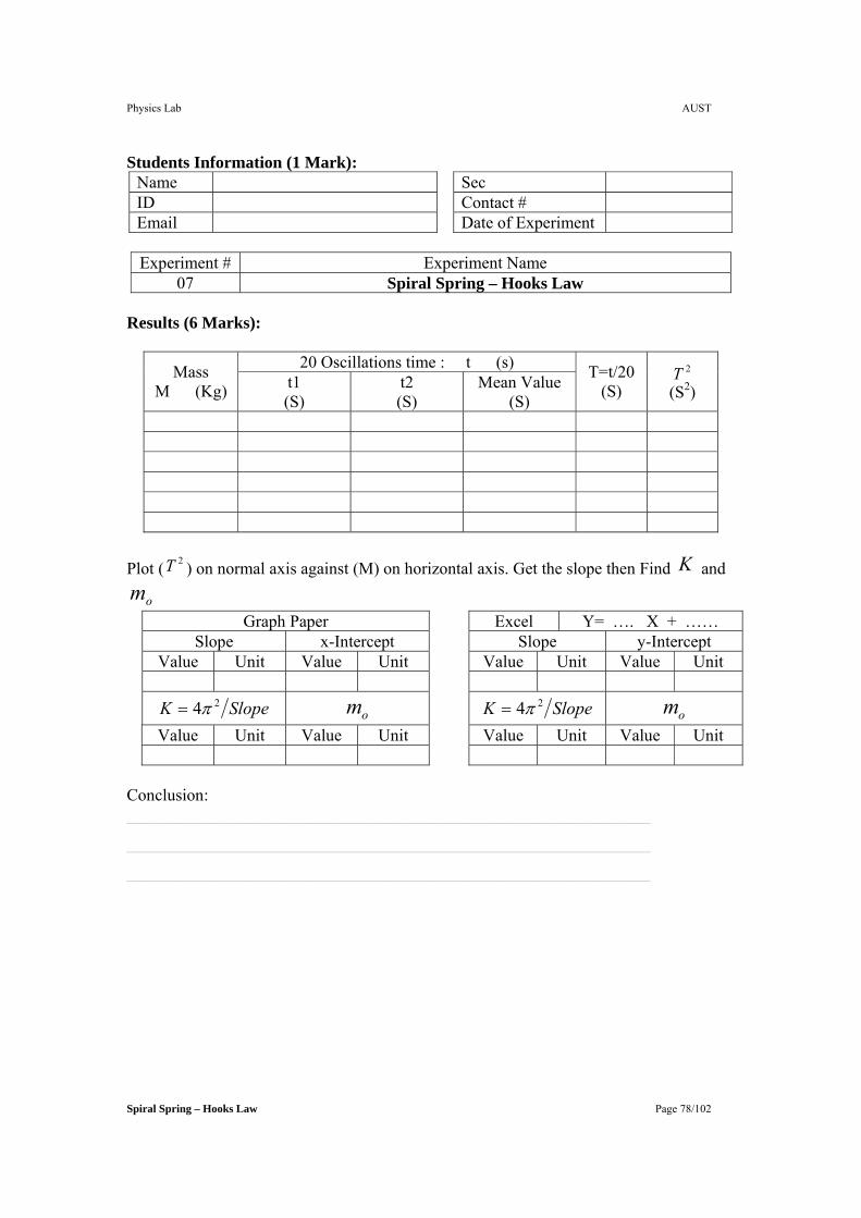
Physics Lab AUST
Spiral Spring – Hooks Law Page 78/102
Students Information (1 Mark): Name Sec ID Contact # Email Date of Experiment
Experiment # Experiment Name
07 Spiral Spring – Hooks Law Results (6 Marks):
20 Oscillations time : t (s) Mass M (Kg) t1
(S) t2 (S)
Mean Value (S)
T=t/20 (S)
2T (S2)
Plot ( 2T ) on normal axis against (M) on horizontal axis. Get the slope then Find K and
om Y= …. X + …… Excel Graph Paper
y-Intercept Slope x-Intercept Slope Unit Value Unit Value Unit Value Unit Value
om SlopeK 24π= om SlopeK 24π= Unit Value Unit Value Unit Value Unit Value
Conclusion: ______________________________________________________________
______________________________________________________________
______________________________________________________________
Physics Lab AUST
Spiral Spring – Hooks Law Page 79/102
Discussion (3 Marks): Q1: If the amplitude of the vibration for a spring is doubled, what happens to the period?
Answer this question by measuring the period of an oscillating 250 gram mass whose
amplitudes of vibration are 2 cm, 4 cm, and 8 cm.
______________________________________________________________
______________________________________________________________
______________________________________________________________
______________________________________________________________
______________________________________________________________
______________________________________________________________
Q2: Choose End points or Equilibrium point for each question.
Question End points
Equilibrium point
At which point(s) does the mass on a vibrating spring have the greatest acceleration?
At which point(s) does it have the least acceleration? At which point(s) does the mass have the largest force exerted on it?
At which point(s) does the mass have the smallest force exerted on it?
At which point(s) does the mass on a vibrating spring have its largest velocity?
At which point(s) does the mass have its smallest velocity?
Q3: You will do this experiment on the moon. What is the result of spring constant K in
this case? Why?
______________________________________________________________
______________________________________________________________
______________________________________________________________
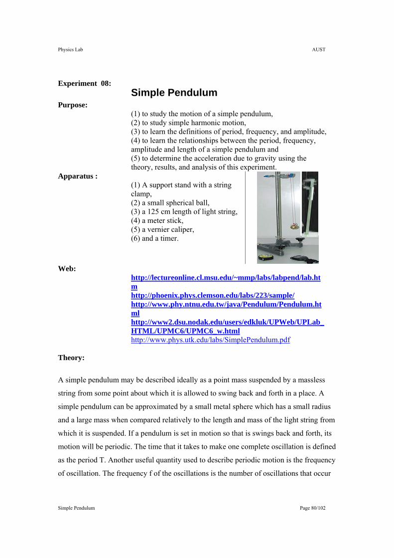
Physics Lab AUST
Simple Pendulum Page 80/102
Experiment 08:
Simple Pendulum Purpose:
(1) to study the motion of a simple pendulum, (2) to study simple harmonic motion, (3) to learn the definitions of period, frequency, and amplitude, (4) to learn the relationships between the period, frequency, amplitude and length of a simple pendulum and (5) to determine the acceleration due to gravity using the theory, results, and analysis of this experiment.
Apparatus : (1) A support stand with a string clamp, (2) a small spherical ball, (3) a 125 cm length of light string, (4) a meter stick, (5) a vernier caliper, (6) and a timer.
Web:
http://lectureonline.cl.msu.edu/~mmp/labs/labpend/lab.htm http://phoenix.phys.clemson.edu/labs/223/sample/ http://www.phy.ntnu.edu.tw/java/Pendulum/Pendulum.html http://www2.dsu.nodak.edu/users/edkluk/UPWeb/UPLab_HTML/UPMC6/UPMC6_w.html http://www.phys.utk.edu/labs/SimplePendulum.pdf
Theory:
A simple pendulum may be described ideally as a point mass suspended by a massless
string from some point about which it is allowed to swing back and forth in a place. A
simple pendulum can be approximated by a small metal sphere which has a small radius
and a large mass when compared relatively to the length and mass of the light string from
which it is suspended. If a pendulum is set in motion so that is swings back and forth, its
motion will be periodic. The time that it takes to make one complete oscillation is defined
as the period T. Another useful quantity used to describe periodic motion is the frequency
of oscillation. The frequency f of the oscillations is the number of oscillations that occur
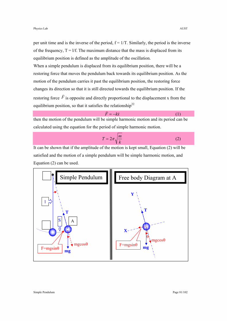
Physics Lab AUST
Simple Pendulum Page 81/102
per unit time and is the inverse of the period, f = 1/T. Similarly, the period is the inverse
of the frequency, T = l/f. The maximum distance that the mass is displaced from its
equilibrium position is defined as the amplitude of the oscillation.
When a simple pendulum is displaced from its equilibrium position, there will be a
restoring force that moves the pendulum back towards its equilibrium position. As the
motion of the pendulum carries it past the equilibrium position, the restoring force
changes its direction so that it is still directed towards the equilibrium position. If the
restoring force Fv
is opposite and directly proportional to the displacement x from the
equilibrium position, so that it satisfies the relationship22
xkF vv−= (1)
then the motion of the pendulum will be simple harmonic motion and its period can be
calculated using the equation for the period of simple harmonic motion.
kmT π2= (2)
It can be shown that if the amplitude of the motion is kept small, Equation (2) will be
satisfied and the motion of a simple pendulum will be simple harmonic motion, and
Equation (2) can be used.
A
l
S
F=mgsinθ mgcosθ
mg
Simple Pendulum
T
Free body Diagram at A
θ
Y
F=mgsinθ mgcosθ
mg
X
T
Physics Lab AUST
Simple Pendulum Page 82/102
The restoring force for a simple pendulum is supplied by the vector sum of the
gravitational force on the mass. mg, and the tension in the string, T. The magnitude of the
restoring force depends on the gravitational force and the displacement of the mass from
the equilibrium position. Where a mass m is suspended by a string of length l and is
displaced from its equilibrium position O by an angle θ and a distance x along the arc OA
through which the mass moves. The gravitational force can be resolved into two
components, one along the radial direction, away from the point of suspension, and one
along the arc in the direction that the mass moves. The component of the gravitational
force along the arc AO provides the restoring force F and is given by
θsinmgF −=v
(3) where g is the acceleration of gravity, θ is the angle the pendulum is displaced, and the
minus sign indicates that the force is opposite to the displacement. For small amplitudes
where θ is small, sinθ can be approximated by θ measured in radians so that Equation (3)
can be written as
θmgF −=v
(4)
The angle θ in radians is lx the arc length divided by the length of the pendulum or the
radius of the circle in which the mass moves. The restoring force is then given by
lxmgF −=
v (5)
and is directly proportional to the displacement x and is in the form of Equation (1) where
k =l
mg . Substituting this value of k into Equation (2), the period of a simple pendulum
can be found by
⎟⎠⎞
⎜⎝⎛
=
lmgmT π2 (6)
and
glT π2= (7)
Therefore, for small amplitudes the period of a simple pendulum depends only on its
length and the value of the acceleration due to gravity.
Physics Lab AUST
Simple Pendulum Page 83/102
Procedure23:
15. The simple pendulum is composed of a small spherical ball suspended by a long,
light string which is attached to a support stand by a string clamp. The string
should be approximately 125 cm long and should be clamped by the string clamp
between the two flat pieces of metal so that the string always pivots about the
same point.
16. Use a vernier caliper to measure the diameter d of the spherical ball and from this
calculate its radius r. Record the values of the diameter and radius in meters.
17. Adjust the length of the pendulum to about 50 cm. The length of the simple
pendulum is the distance from the point of suspension to the center of the ball.
Measure the length of the string ls from the point of suspension to the top of the
ball using a meter stick. Add the radius of the ball to the string length ls and
record that value as the length of the pendulum L=ls +r.
18. Displace the pendulum about 5º from its equilibrium position and let it swing
back and forth. Measure twice the total time that it takes to make 20 complete
oscillations. Record that time in your table.
19. Increase the length of the pendulum by about 0.20 m and repeat the measurements
made in the previous steps until the length increases to approximately 1.5 m.
20. Calculate the period of the oscillations for each length by dividing the total mean
time value by the number of oscillations, 20. Record the values in the appropriate
column of your data table.
21. On Excel: Graph the period of the pendulum as a function of its length using the
chart feature of Excel. The length of the pendulum is the independent variable and
should be plotted on the horizontal axis or abscissa (x axis). The period is the
dependent variable and should be plotted on the vertical axis or ordinate (y axis).
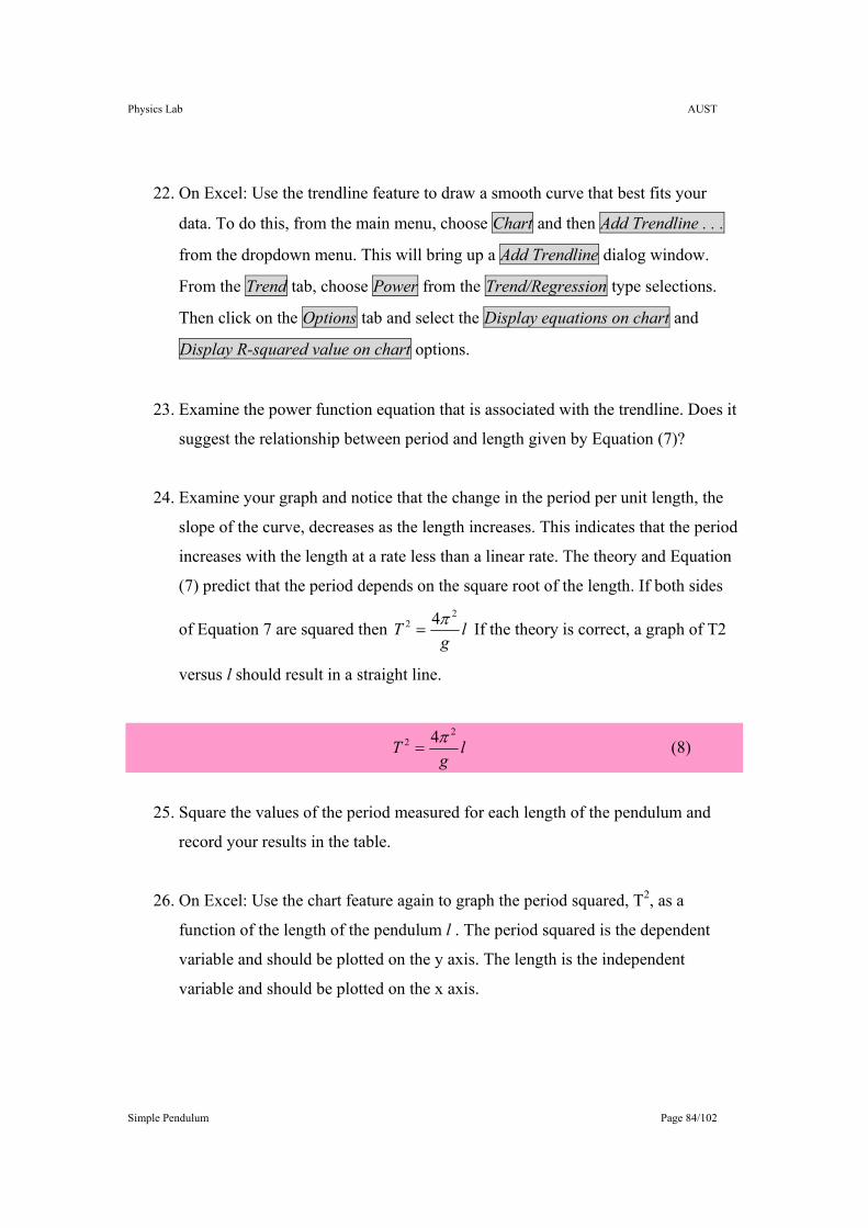
Physics Lab AUST
Simple Pendulum Page 84/102
22. On Excel: Use the trendline feature to draw a smooth curve that best fits your
data. To do this, from the main menu, choose Chart and then Add Trendline . . .
from the dropdown menu. This will bring up a Add Trendline dialog window.
From the Trend tab, choose Power from the Trend/Regression type selections.
Then click on the Options tab and select the Display equations on chart and
Display R-squared value on chart options.
23. Examine the power function equation that is associated with the trendline. Does it
suggest the relationship between period and length given by Equation (7)?
24. Examine your graph and notice that the change in the period per unit length, the
slope of the curve, decreases as the length increases. This indicates that the period
increases with the length at a rate less than a linear rate. The theory and Equation
(7) predict that the period depends on the square root of the length. If both sides
of Equation 7 are squared then lg
T2
2 4π= If the theory is correct, a graph of T2
versus l should result in a straight line.
lg
T2
2 4π= (8)
25. Square the values of the period measured for each length of the pendulum and
record your results in the table.
26. On Excel: Use the chart feature again to graph the period squared, T2, as a
function of the length of the pendulum l . The period squared is the dependent
variable and should be plotted on the y axis. The length is the independent
variable and should be plotted on the x axis.
Physics Lab AUST
Simple Pendulum Page 85/102
27. Examine your graph of T2 versus l and check to see if there is a linear relationship
between T2 and l so that the data points lie along a line.
28. On Excel: Use the trendline feature to perform a linear regression to find a
straight line that best fits your data points. This time from the Add Trendline
dialog window. Choose Linear from the Trend/Regression type selections. Click
on the Options tab and once again select the Display equations on chart , Display
R-squared value on chart and set intercept =0 options. This should draw a
straight line through origin that best fits the data and should display the equation
for this straight line.
29. On Excel: Equation (8) , lg
T2
2 4π= , is of the form y=ax where y= T2 and a=
g
24π , x= l . A graph of T2 versus l should therefore result in a straight line whose
slope, a, is equal to g
24π . From the equation for the trendline, record the value
for the slope, a, and from the equation a= g
24π find g, the acceleration due to
gravity, which represent calculated value practicalg .
30. On Graph Paper: Plot ( 2T )on normal axis against (L) on horizontal axis. Get the
slope then Find practicalg .
31. Compare your result with the expected value of the acceleration due to gravity 9.8
m/ s2. Calculate the Percent Error in your result and the accepted result.
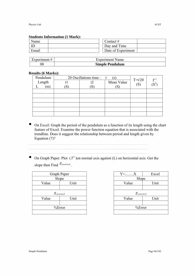
Physics Lab AUST
Simple Pendulum Page 86/102
Students Information (1 Mark): Name Contact # ID Day and Time Email Date of Experiment
Experiment # Experiment Name
08 Simple Pendulum Results (6 Marks):
20 Oscillations time : t (s) Pendulum Length
L (m) t1 (S)
t2 (S)
Mean Value (S)
T=t/20 (S)
2T (S2)
On Excel: Graph the period of the pendulum as a function of its length using the chart feature of Excel. Examine the power function equation that is associated with the trendline. Does it suggest the relationship between period and length given by Equation (7)?
______________________________________________________________ ______________________________________________________________ ______________________________________________________________
On Graph Paper: Plot ( 2T )on normal axis against (L) on horizontal axis. Get the
slope then Find practicalg .
Excel Y=…….X Graph Paper Slope Slope
Unit Value Unit Value
practicalg practicalg Unit Value Unit Value
%Error %Error
Physics Lab AUST
Simple Pendulum Page 87/102
Discussion (3 Marks): Q1: Discuss your errors: ______________________________________________________________
______________________________________________________________
______________________________________________________________
Q2: At °20 angle, I can not apply the same formula. Why? ______________________________________________________________
______________________________________________________________
______________________________________________________________
Q3: Use three different weights of pendulum, and measure the oscillation time. From your results, is oscillation time increase or decrease (support your answer with expected result and calculated result). A. Discuss theoretical (Expected) Result: ______________________________________________________________
______________________________________________________________
______________________________________________________________
B. Discuss practical results: ______________________________________________________________
______________________________________________________________
______________________________________________________________
______________________________________________________________
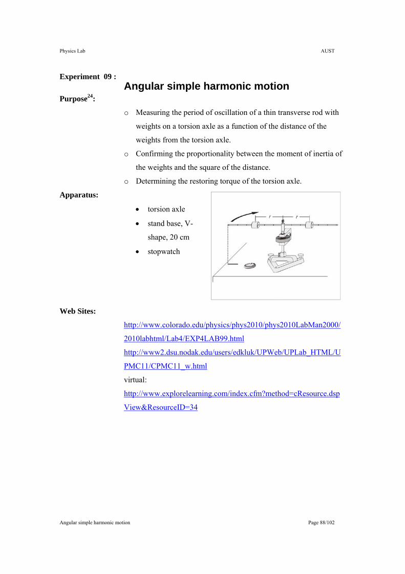
Physics Lab AUST
Angular simple harmonic motion Page 88/102
Experiment 09 : Angular simple harmonic motion
Purpose24:
o Measuring the period of oscillation of a thin transverse rod with
weights on a torsion axle as a function of the distance of the
weights from the torsion axle.
o Confirming the proportionality between the moment of inertia of
the weights and the square of the distance.
o Determining the restoring torque of the torsion axle.
Apparatus:
• torsion axle
• stand base, V-
shape, 20 cm
• stopwatch
Web Sites:
http://www.colorado.edu/physics/phys2010/phys2010LabMan2000/
2010labhtml/Lab4/EXP4LAB99.html
http://www2.dsu.nodak.edu/users/edkluk/UPWeb/UPLab_HTML/U
PMC11/CPMC11_w.html
virtual:
http://www.explorelearning.com/index.cfm?method=cResource.dsp
View&ResourceID=34
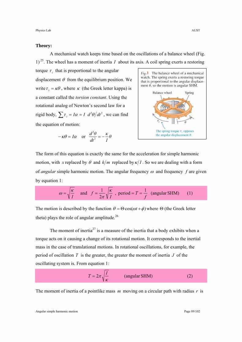
Physics Lab AUST
Angular simple harmonic motion Page 89/102
Theory:
A mechanical watch keeps time based on the oscillations of a balance wheel (Fig.
1) 25. The wheel has a moment of inertia I about its axis. A coil spring exerts a restoring
torque zτ that is proportional to the angular
displacement θ from the equilibrium position. We
write κθτ =z , where κ (the Greek letter kappa) is
a constant called the torsion constant. Using the
rotational analog of Newton’s second law for a
rigid body, 22 dtdIIz θατ ==∑ , we can find
the equation of motion:
θIκ
dtθdI −==− 2
2
or ακθ
The form of this equation is exactly the same for the acceleration for simple harmonic
motion, with x replaced by θ and mk replaced by Iκ . So we are dealing with a form
of angular simple harmonic motion. The angular frequency ω and frequency f are given
by equation 1:
SHM)(angular 1period , 21 and
fT
If
I====
κπ
κω (1)
The motion is described by the function )cos( φωθ +Θ= t where Θ (the Greek letter
theta) plays the role of angular amplitude.26
The moment of inertia27 is a measure of the inertia that a body exhibits when a
torque acts on it causing a change of its rotational motion. It corresponds to the inertial
mass in the case of translational motions. In rotational oscillations, for example, the
period of oscillation T is the greater, the greater the moment of inertia J of the
oscillating system is. From equation 1:
SHM)(angular 2 κ
π IT = (2)
The moment of inertia of a pointlike mass m moving on a circular path with radius r is
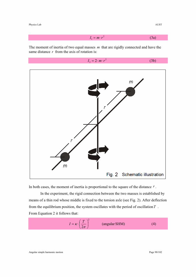
Physics Lab AUST
Angular simple harmonic motion Page 90/102
21 rmI ⋅= (3a)
The moment of inertia of two equal masses m that are rigidly connected and have the same distance r from the axis of rotation is:
22 2 rmI ⋅⋅= (3b)
In both cases, the moment of inertia is proportional to the square of the distance r .
In the experiment, the rigid connection between the two masses is established by
means of a thin rod whose middle is fixed to the torsion axle (see Fig. 2). After deflection
from the equilibrium position, the system oscillates with the period of oscillationT .
From Equation 2 it follows that:
SHM)(angular 2
2
⎟⎠⎞
⎜⎝⎛⋅=π
κ TI (4)
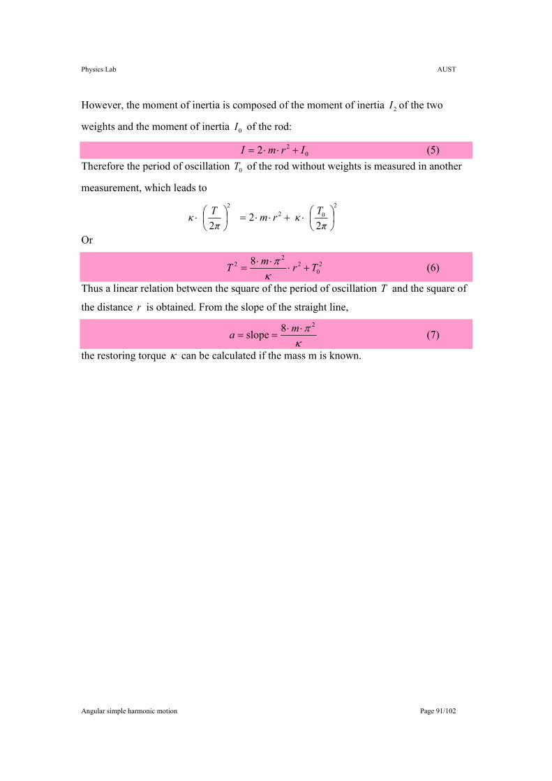
Physics Lab AUST
Angular simple harmonic motion Page 91/102
However, the moment of inertia is composed of the moment of inertia 2I of the two
weights and the moment of inertia 0I of the rod:
022 IrmI +⋅⋅= (5)
Therefore the period of oscillation 0T of the rod without weights is measured in another
measurement, which leads to
π
T κrm π
T κ2
022
22
2⎟⎠⎞
⎜⎝⎛⋅+⋅⋅=⎟
⎠⎞
⎜⎝⎛⋅
Or
20
22
2 8 TrmT +⋅⋅⋅
=κπ (6)
Thus a linear relation between the square of the period of oscillation T and the square of
the distance r is obtained. From the slope of the straight line,
8slope 2
κπ⋅⋅
==ma (7)
the restoring torque κ can be calculated if the mass m is known.
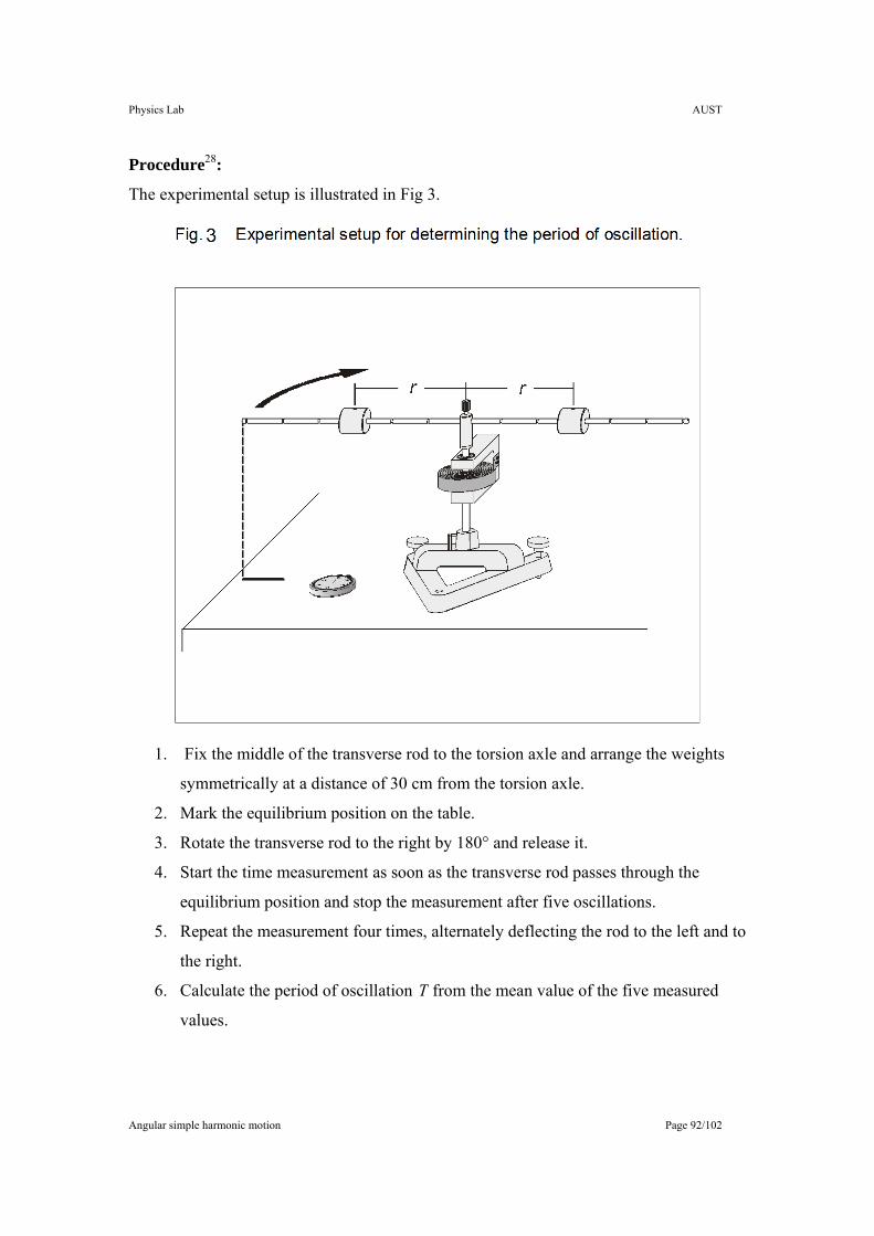
Physics Lab AUST
Angular simple harmonic motion Page 92/102
Procedure28:
The experimental setup is illustrated in Fig 3.
1. Fix the middle of the transverse rod to the torsion axle and arrange the weights
symmetrically at a distance of 30 cm from the torsion axle.
2. Mark the equilibrium position on the table.
3. Rotate the transverse rod to the right by 180° and release it.
4. Start the time measurement as soon as the transverse rod passes through the
equilibrium position and stop the measurement after five oscillations.
5. Repeat the measurement four times, alternately deflecting the rod to the left and to
the right.
6. Calculate the period of oscillation T from the mean value of the five measured
values.
Physics Lab AUST
Angular simple harmonic motion Page 93/102
7. One after another reduce the distance to 25 cm, 20 cm, 15 cm, 10 cm and 5 cm,
each time repeating the measurement.
8. Remove the weights, and repeat the measurement.
9. Calculate 2r and 2T for each r . Record the values in the appropriate column of
your data table.
10. On Graph paper: Plot a graph of 2T vs. 2r , and determine the torsion constant κ
from the relationship of ( ) slope8 2πκ ⋅⋅= m of this line.
11. On Excel: Use the chart feature to graph the period squared, 2T , as a function of
the square of the distance 2r . The period squared is the dependent variable and
should be plotted on the y axis. The square of the distance is the independent
variable and should be plotted on the x axis.
12. On Excel: Examine your graph of 2T versus 2r and check to see if there is a linear
relationship between 2T and 2r so that the data points lie along a line. Use the
trendline feature to perform a linear regression to find a straight line that best fits
your data points. From the Add Trendline dialog window. Choose Linear from
the Trend/Regression type selections. Click on the Options tab and once again
select the Display equations on chart and Display R-squared value on chart
options. This should draw a straight line (not through origin) that best fits the data
and should display the equation for this straight line.
13. On Excel: Equation (6) is of the form baxy += where 2Ty = and
( ) 8 2 κπ⋅⋅= ma , 20aTb = , 2rx = . A graph of 2T versus 2r should therefore
result in a straight line whose slope, a, is equal to ( ) 8 2 κπ⋅⋅m . From the
equation for the trendline, record the value for the slope, a, the interception, b.
From the equation ( ) 8 2 κπ⋅⋅= ma findκ , the torsion constant.
14. Get the percentage errors for each shape, if you know that Nm023.0expected =κ
where ( )[ ] %100% ⋅−= ExpectedCalcultedExpectederror .
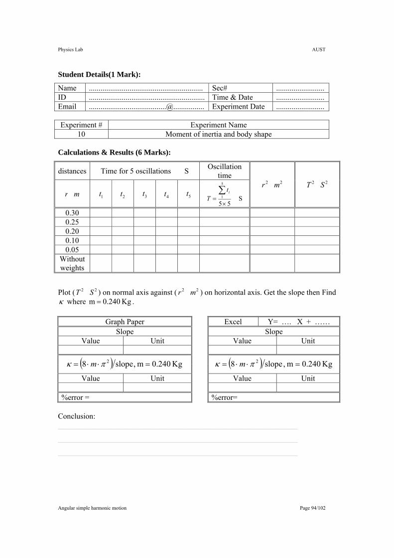
Physics Lab AUST
Angular simple harmonic motion Page 94/102
Student Details(1 Mark):
Name ........................................................... Sec# ......................... ID ............................................................ Time & Date ......................... Email ........................................@................ Experiment Date ......................... Experiment # Experiment Name
10 Moment of inertia and body shape Calculations & Results (6 Marks):
distances Time for 5 oscillations S Oscillation time
mr 1t 2t 3t 4t 5t S
55
5
1
×=∑ it
T
22 mr 22 ST
0.30 0.25 0.20 0.10 0.05
Without weights
Plot ( 22 ST ) on normal axis against ( 22 mr ) on horizontal axis. Get the slope then Find κ where Kg 0.240m = .
Graph Paper Excel Y= …. X + …… Slope Slope
Value Unit Value Unit
( ) Kg 0.240m ,slope8 2 =⋅⋅= πκ m ( ) Kg 0.240m ,slope8 2 =⋅⋅= πκ m
Value Unit Value Unit
%error = %error= Conclusion: ______________________________________________________________
______________________________________________________________
______________________________________________________________
Physics Lab AUST
Angular simple harmonic motion Page 95/102
Discussion (3 Marks):
1. Discuss the %error of each item:
______________________________________________________________
______________________________________________________________
______________________________________________________________
______________________________________________________________
______________________________________________________________
______________________________________________________________
2. Using same setup: Can I use equation 4 to find the mass of solid sphere on some
spaceship where there is no gravity? How?( mRRmI esolidspher 145.02 ,..52 2 == )
______________________________________________________________
______________________________________________________________
=m __________________________________________________________
3. Did A hollow body and a solid body with same mass make the same T. Why?
______________________________________________________________
______________________________________________________________
______________________________________________________________
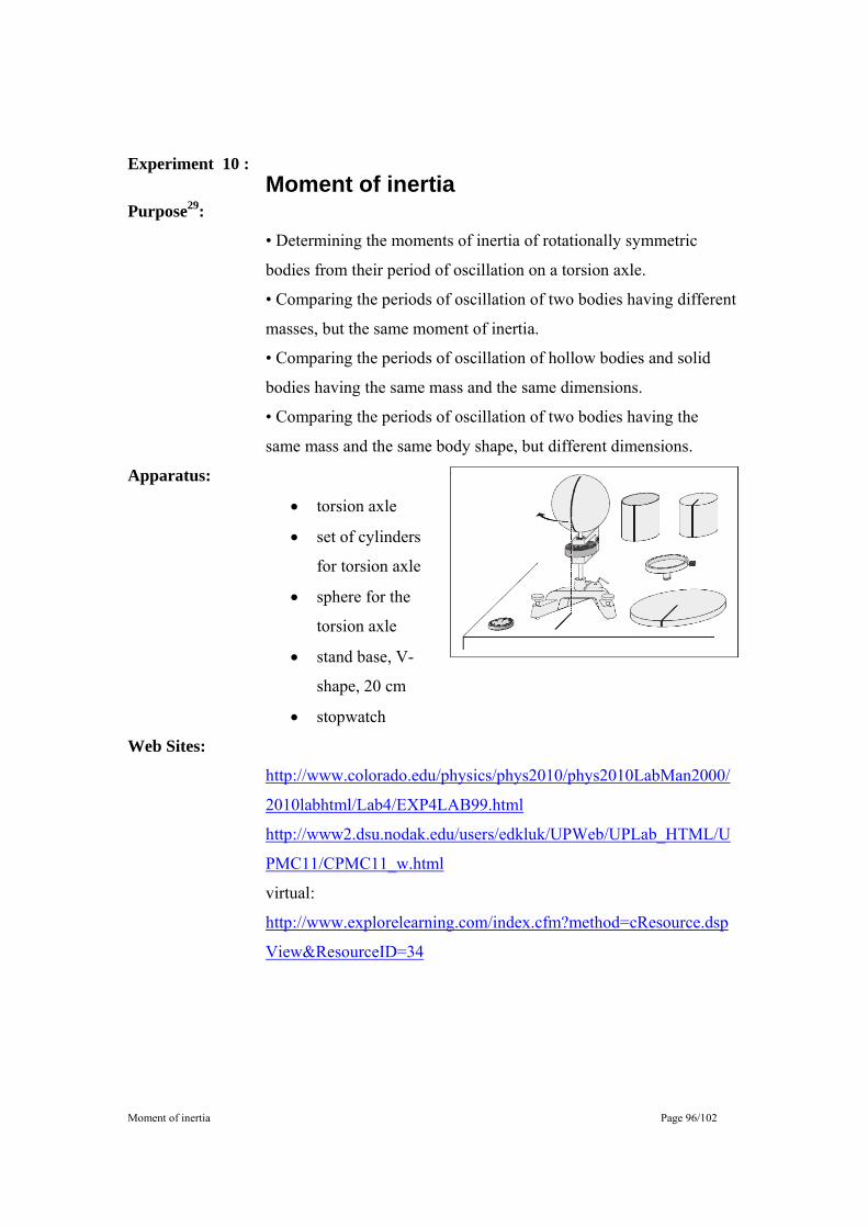
Moment of inertia Page 96/102
Experiment 10 : Moment of inertia
Purpose29:
• Determining the moments of inertia of rotationally symmetric
bodies from their period of oscillation on a torsion axle.
• Comparing the periods of oscillation of two bodies having different
masses, but the same moment of inertia.
• Comparing the periods of oscillation of hollow bodies and solid
bodies having the same mass and the same dimensions.
• Comparing the periods of oscillation of two bodies having the
same mass and the same body shape, but different dimensions.
Apparatus:
• torsion axle
• set of cylinders
for torsion axle
• sphere for the
torsion axle
• stand base, V-
shape, 20 cm
• stopwatch
Web Sites:
http://www.colorado.edu/physics/phys2010/phys2010LabMan2000/
2010labhtml/Lab4/EXP4LAB99.html
http://www2.dsu.nodak.edu/users/edkluk/UPWeb/UPLab_HTML/U
PMC11/CPMC11_w.html
virtual:
http://www.explorelearning.com/index.cfm?method=cResource.dsp
View&ResourceID=34
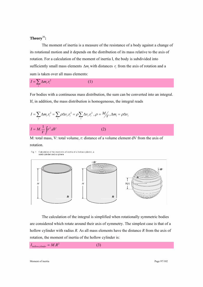
Moment of inertia Page 97/102
Theory30:
The moment of inertia is a measure of the resistance of a body against a change of
its rotational motion and it depends on the distribution of its mass relative to the axis of
rotation. For a calculation of the moment of inertia I, the body is subdivided into
sufficiently small mass elements im∆ with distances ir from the axis of rotation and a
sum is taken over all mass elements:
(1) . 2∑∆=i
ii rmI
For bodies with a continuous mass distribution, the sum can be converted into an integral.
If, in addition, the mass distribution is homogeneous, the integral reads
iii
iiiii
ii vmVMrvrvrmI ∆=∆=∆=∆=∆= ∑∑∑ ρρρρ , , ... 2
i
22
(2) .1. 2∫=V
dVrV
MI
M: total mass, V: total volume, r: distance of a volume element dV from the axis of
rotation.
The calculation of the integral is simplified when rotationally symmetric bodies
are considered which rotate around their axis of symmetry. The simplest case is that of a
hollow cylinder with radius R. As all mass elements have the distance R from the axis of
rotation, the moment of inertia of the hollow cylinder is:
(3) . 2RMI nderhollowcyli =
Moment of inertia Page 98/102
In the case of a solid cylinder with equal mass M and equal radius R, Eq. (2) leads
to the formula:
.Hπ.RVdrHrrV
MIR
dersolidcylin2
0
2 with ...2.1. == ∫ π and the result is:
(4) ..21 2RMI dersolidcylin =
That means, the moment of inertia of a solid cylinder is smaller than that of the
hollow cylinder as the distances of the mass elements from the axis of rotation are
between 0 and R.
An even smaller value is expected for the moment of inertia of a solid sphere with
radius R (see Fig. 1). In this case, Eq. (2) leads to the formula:
3
0
222
34 with ...2.1. π.RVdrrRrr
VMI
R
esolidspher =−= ∫ π
(5) ..52 2RMI esolidspher =
Thus, apart form the mass M and the radius R of the bodies under consideration a
dimensionless factor enters the calculation of the moment of inertia, which depends on
the shape of the respective body.
The moment of inertia is determined from the period of oscillation of a torsion
axle, on which the test body is fixed and which is connected elastically to the stand via a
helical spring. The system is excited to perform harmonic oscillations. If the restoring
torque κ is known, the moment of inertia of the test body is calculated from the period
of oscillation T according to:
(6) 2
.2
⎟⎠⎞
⎜⎝⎛=π
κ TI
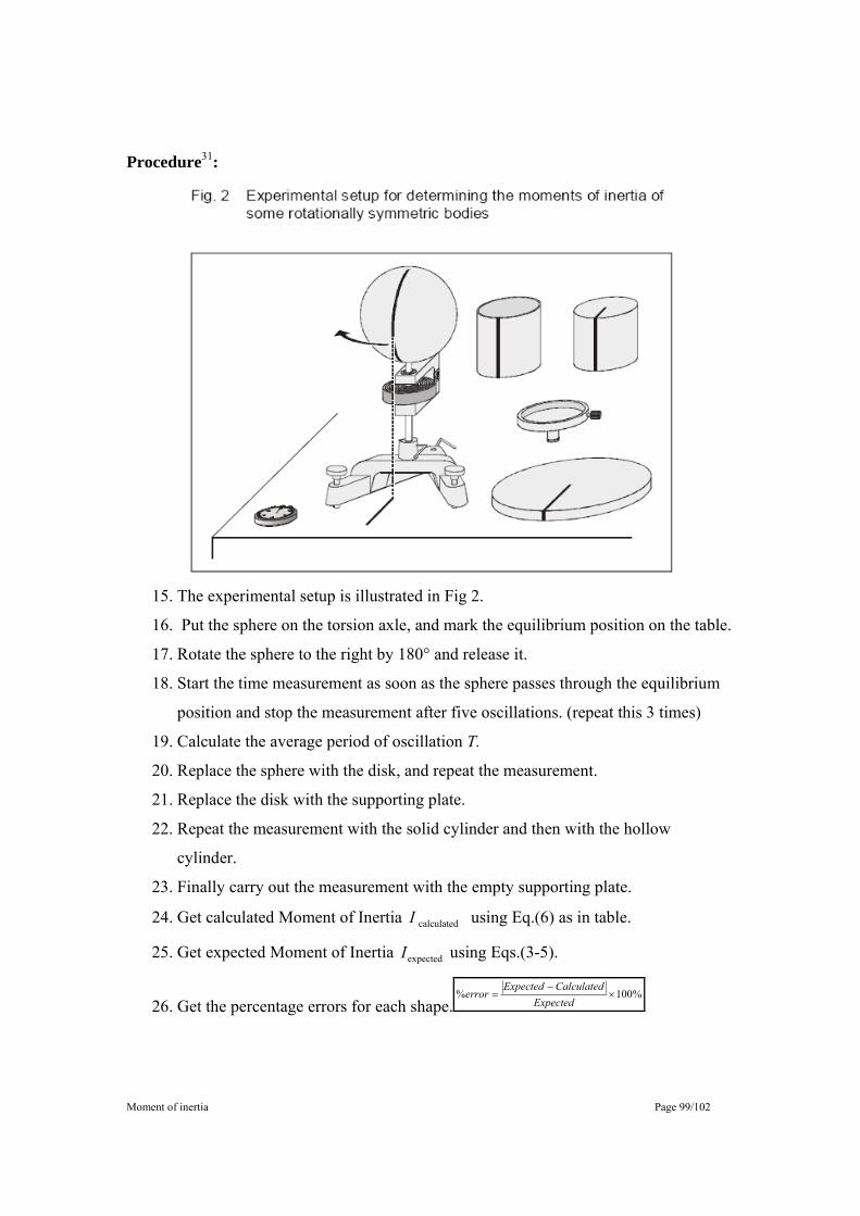
Moment of inertia Page 99/102
Procedure31:
15. The experimental setup is illustrated in Fig 2.
16. Put the sphere on the torsion axle, and mark the equilibrium position on the table.
17. Rotate the sphere to the right by 180° and release it.
18. Start the time measurement as soon as the sphere passes through the equilibrium
position and stop the measurement after five oscillations. (repeat this 3 times)
19. Calculate the average period of oscillation T.
20. Replace the sphere with the disk, and repeat the measurement.
21. Replace the disk with the supporting plate.
22. Repeat the measurement with the solid cylinder and then with the hollow
cylinder.
23. Finally carry out the measurement with the empty supporting plate.
24. Get calculated Moment of Inertia calculated I using Eq.(6) as in table.
25. Get expected Moment of Inertia expectedI using Eqs.(3-5).
26. Get the percentage errors for each shape.%100% ×
−=
ExpectedCalculatedExpected
error
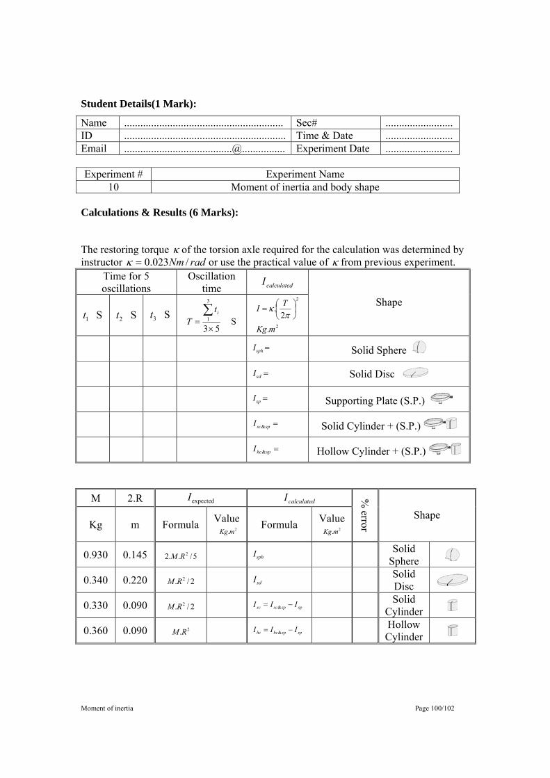
Moment of inertia Page 100/102
Student Details(1 Mark):
Name ........................................................... Sec# ......................... ID ............................................................ Time & Date ......................... Email ........................................@................ Experiment Date ......................... Experiment # Experiment Name
10 Moment of inertia and body shape Calculations & Results (6 Marks):
The restoring torque κ of the torsion axle required for the calculation was determined by instructor radNm /023.0=κ or use the practical value of κ from previous experiment.
Time for 5 oscillations
Oscillation time calculatedI
S 1t S 2t S 3t S
53
3
1
×=∑ it
T 2
2
.2
.
mKg
TI ⎟⎠⎞
⎜⎝⎛=π
κ Shape
=sphI Solid Sphere =sdI Solid Disc
=spI Supporting Plate (S.P.) & =spscI Solid Cylinder + (S.P.) & =sphcI Hollow Cylinder + (S.P.)
M 2.R expectedI calculatedI
Kg m Formula Value 2.mKg Formula Value
2.mKg
% error
Shape
0.930 0.145 5/..2 2RM sphI Solid Sphere
0.340 0.220 2/. 2RM sdI Solid Disc
0.330 0.090 2/. 2RM spspscsc III −= & Solid
Cylinder
0.360 0.090 2.RM spsphchc III −= & Hollow
Cylinder
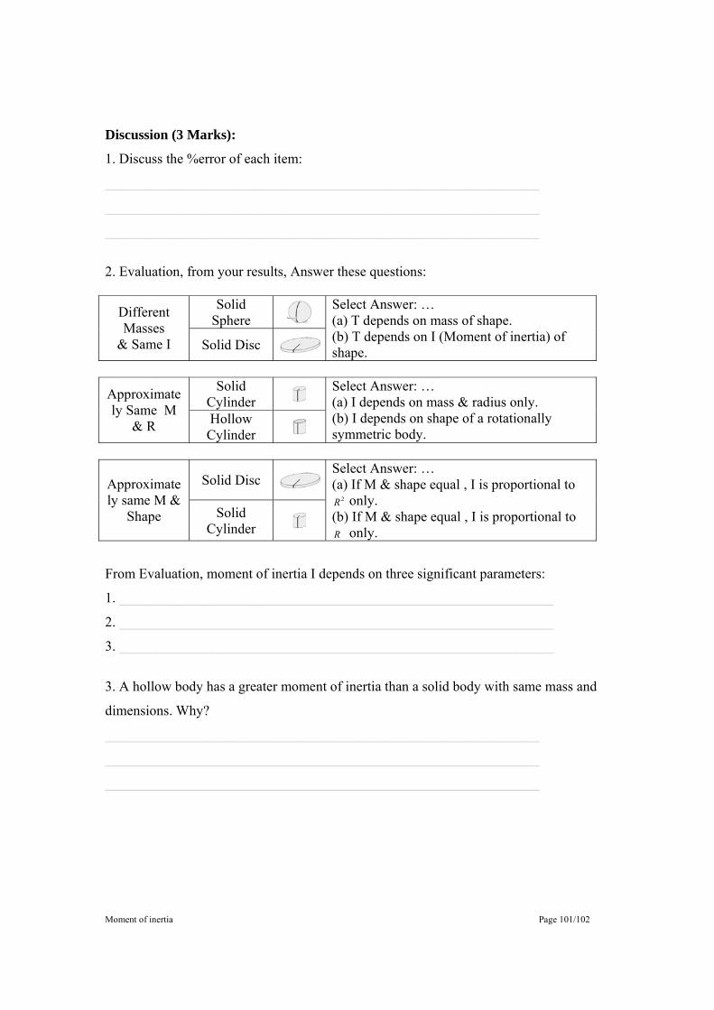
Moment of inertia Page 101/102
Discussion (3 Marks):
1. Discuss the %error of each item:
______________________________________________________________
______________________________________________________________
______________________________________________________________
2. Evaluation, from your results, Answer these questions:
Solid Sphere Different
Masses & Same I Solid Disc
Select Answer: … (a) T depends on mass of shape. (b) T depends on I (Moment of inertia) of shape.
Solid
Cylinder Approximately Same M
& R Hollow Cylinder
Select Answer: … (a) I depends on mass & radius only. (b) I depends on shape of a rotationally symmetric body.
Solid Disc Approximately same M &
Shape Solid Cylinder
Select Answer: … (a) If M & shape equal , I is proportional to
2R only. (b) If M & shape equal , I is proportional to R only.
From Evaluation, moment of inertia I depends on three significant parameters:
1. ______________________________________________________________
2. ______________________________________________________________
3. ______________________________________________________________
3. A hollow body has a greater moment of inertia than a solid body with same mass and
dimensions. Why?
______________________________________________________________
______________________________________________________________
______________________________________________________________

References page 102/102
1 According the web site of the book: H.C. Ohanian and J.T.Markert, “Physics for engineers and scientists” , 3rd edition, W. W. NORTON & COMPANY STUDYSPACE. Website is : http://www.wwnorton.com/college/physics/om/_content/_index/tutorials.shtml 2 According the web site of the book: H.C. Ohanian and J.T.Markert, “Physics for engineers and scientists” , 3rd edition, W. W. NORTON & COMPANY STUDYSPACE. Website is : http://www.wwnorton.com/college/physics/om/_content/_index/tutorials.shtml 3 http://www.ece.uwaterloo.ca/~ece204/TheBook/06LeastSquares/ 4 http://www.people.ex.ac.uk/SEGLea/psy2005/simpreg.html 5 http://people.hofstra.edu/stefan_waner/realworld/calctopic1/regression.html 6 http://online.redwoods.cc.ca.us/instruct/mbutler/BUTLER/math99/ppt/graphs.pdf 7 Photos here (graphing Lab) are a screen snapshot from Microsoft office excel 2003 8 All photos here (Graphing Lab) From website http://www.phy.uct.ac.za/courses/c1lab/vernier1.html 9 From http://www.leybold-didactic.com/literatur/hb/e/p1/p1251_e.pdf 10 These figures (vectors exp.) are from http://www.physchem.co.za/Vectors/Addition.htm 11 The colored 3d-inclined plane (Motion Along Straight line exp.) was designed by A.D.Mahir using Google sketch up software. 12 Young & Freedman , “University physics with modern physics”, 12th ed., Pearson/Addison Wesley, 2008, p326 13 From http://www.leybold-didactic.com/literatur/hb/e/p1/p1261_e.pdf 14 Young, and Freedman, "University physics with modern physics", 12ed. Pearson/Addison Wesley, 2008, p 149-155. 15 Young, and Freedman, "University physics with modern physics", 12ed. Pearson/Addison Wesley, 2008, p 149. 16 Young, and Freedman, "University physics with modern physics", 12ed. Pearson/Addison Wesley, 2008, p 151. 17 Young, and Freedman, "University physics with modern physics", 12ed. Pearson/Addison Wesley, 2008, p 150. 18 From http://www.leybold-didactic.com/literatur/hb/e/p1/p1261_e.pdf , http://www.leybold-didactic.com/literatur/s1/e/d1/d1241_e.pdf, http://www.leybold-didactic.com/literatur/s1/e/d1/d1242_e.pdf 19 Young & Freedman, “University physics with modern physics”, 12th ed, Pearson AW, 2008, P421-427 20 From http://hyperphysics.phy-astr.gsu.edu/hbase/shm.html 21 Some of procedure steps are coming from http://www.phys.utk.edu/labs/SimplePendulum.pdf 22 From http://www.phys.utk.edu/labs/SimplePendulum.pdf and Young & Freedman, “University physics with modern physics”, 12th ed, Pearson/Addison Wesley, 2008, P421-427 23 Some of procedure steps are coming from http://www.phys.utk.edu/labs/SimplePendulum.pdf 24 From http://www.leybold-didactic.com/literatur/hb/e/p1/p1451_e.pdf 25 From Young and Freedman, “University physics with modern physics”, 12th ed, Pearson/Addison Wesley, 2008.pages: 433 26 Young and Freedman, “University physics with modern physics”, 12th ed, Pearson/Addison Wesley, 2008.pages: 433-434 27 http://www.ld-online.de/literatur/hb/e/p1/p1451_e.pdf page 1 28 http://www.ld-online.de/literatur/hb/e/p1/p1451_e.pdf Page 2 29 From http://www.leybold-didactic.com/literatur/hb/e/p1/p1452_e.pdf Page 1 30 From http://www.leybold-didactic.com/literatur/hb/e/p1/p1452_e.pdf Page 1 31 From http://www.leybold-didactic.com/literatur/hb/e/p1/p1452_e.pdf page 2


