Physics 239 (211C): Quantum phases of matter

Lightning summary of algebraic topology

Spring 2021

Lecturer: McGreevy

These notes live here. Please email corrections and questions to mcgreevy at physics

dot ucsd dot edu.

Last updated: March 23, 2021, 14:09:59

1

Contents

1 Homology 3

1.1 Cell complexes and homology . . . . . . . . . . . . . . . . . . . . . . . 3

1.2 More examples than you need . . . . . . . . . . . . . . . . . . . . . . . 4

1.3 Euler-Poincare theorem . . . . . . . . . . . . . . . . . . . . . . . . . . . 9

1.4 Exact sequences . . . . . . . . . . . . . . . . . . . . . . . . . . . . . . . 10

2 Cohomology 10

2.1 de Rham cohomology . . . . . . . . . . . . . . . . . . . . . . . . . . . . 10

2.2 Cech cohomology . . . . . . . . . . . . . . . . . . . . . . . . . . . . . . 12

3 Homotopy 14

3.1 Notions of ‘same’ . . . . . . . . . . . . . . . . . . . . . . . . . . . . . . 15

3.2 Homotopy equivalence and homology/cohomology . . . . . . . . . . . . 15

3.3 Homotopy groups . . . . . . . . . . . . . . . . . . . . . . . . . . . . . . 16

3.4 Fiber bundles and covering maps . . . . . . . . . . . . . . . . . . . . . 23

3.5 Relative homotopy. . . . . . . . . . . . . . . . . . . . . . . . . . . . . . 26

2

1 Homology

1.1 Cell complexes and homology

Take a d-dimensional manifold X whose topology is of interest and chop it up into

simply-connected cells. By “simply-connected” here I just mean that each cell can be

deformed into a ball. For d = 2 e.g. this means a triangulation (or squarulation or · · · )into a set of 2-cells which are triangles (or squares...), 1-cells which are intervals, and

0-cells which are points. It is what physicists might call a lattice, though no translation

symmetry is actually required or assumed here. But it has more structure – it knows

how it is glued together. This gluing data is encoded in a boundary map ∂, which we

define next. Let ∆k be the set of k-cells in the triangulation of X, and choose an an

abelian group A (e.g. Z2). Define a vector space

Ωk ≡ Ωk(∆, A) ≡ spanAσ ∈ ∆k

to be spanned by vectors associated with k-cells σ, with coefficients in A. (We are

writing the group law of A additively, so e.g . for Z2 it is 1 + 1 = 0.) It does no harm to

introduce an inner product where these vectors σ are orthonormal. An element C ∈ Ωk

is then a formal linear combination of k-cells, and is called a k-chain – it’s important

that we can add (and subtract) k-chains, C + C ′ ∈ Ωk. A k-chain with a negative

coefficient can be regarded as having the opposite orientation.

The boundary map takes the vector space Ωk to the corresponding vector space for

the (k-1)-cells, Ωk−1:

∂k : Ωk → Ωk−1

This map ∂ is linear and takes a basis vector associated with a k-cell to the linear

combination (with signs for orientation and multiplicity) of cells the union of which lie

in its boundary. (And it takes a basis vector associated to a collection of k-cells to the

sum of vectors.) For example, in this figure, wy1y2

y3

we have ∂w = y1−y2+y3

(where I denote the vectors associated with the simplices by the names of the simplices,

why not?). This construction is called a cell complex1. A chain C satisfying ∂C = 0 is

called a cycle, and is said to be closed.

1There are many very closely related constructions (such as simplicial complex or ∆-complex or

semi-simplicial complex or CW-complex) but I will not distinguish between them. One distinction is

that we don’t care that all the cells are triangles or their higher-dimensional generalizations.

3

The fact that the boundary of a boundary is empty makes this series of vector

spaces connected by linear maps into a chain complex, meaning that ∂2 = 0. So the

image of ∂p+1 : Ωp+1 → Ωp is a subspace of ker (∂p : Ωp → Ωp−1). This allows us to

define the homology of this chain complex – equivalence classes of p-cycles, modulo

boundaries of p+ 1 chains:

Hp(∆, A) ≡ ker (∂ : Ωp → ∆p−1) ⊂ Ωp

im (∂ : Ωp+1 → Ωp).

These objects depend only on the topology of X and not on how we chopped it up.

Below we’ll discuss several points of view on this independence of homology on the

triangulation.

Hp(∆, A) is a vector space over A. In the case when A is a field (such as Zp for p

prime) the dimensions of these vector spaces over A are called the Betti numbers of

X. When A is not a field there can be more information called torsion, which we’ll

discuss.

Note that Hp(X,A) is also itself a group. The group law is just addition of rep-

resentatives: if C and C ′ are cycles, then the sum of their equivalence classes modulo

boundaries is [C]+[C ′] = [C+C ′]. This is independent of the choice of representatives.

1.2 More examples than you need

The simplest possible example is complex with only a single 0-cell, a point. This has

H0(pt, A) = A, and all other Hn>0 vanish. If our cell complex were k 0-cells, we would

find H0(k pts, A) = Ak in agreement with the discussion above about ferromagnets.

Circle. Consider the cell complex at top right. This is a cellulation

of a circle with one 1-cell and one 0-cell. The boundary map is ∂e1 =

e0 − e0 = 0. The kernel is everyone and the image is no one. So the

homology (with integer coefficients) is H0(S1, A) = A = H1(S

1, A).

Another cell decomposition of the circle is the bottom figure at right.

Now there are two 1-cells and two 0-cells with boundary map ∂y1 =

p1 − p2 = −∂y2. Now the complex looks like

0→ A2

1 −1

−1 1

→ A2 → 0.

The kernel of ∂ is generated by y1 + y2. The complement of the image is gener-

ated by p1 ' p2 mod ∂. So we find the same answer for the homology as above,

b0(S1) = b1(S

1) = 1.

4

Ball. Consider what happens if we add to the first example a 2-cell e2 whose boundary

is e1 – i.e. fill in the interior of the circle in the picture. This makes a cellulation of a

2-ball. The complex is

0→ A1→ A

0→ A→ 0.

In that case, e1 ∈ Im∂2, so it kills the first homology – Ω1 and Ω2 eat each other. This

complex has the same homology as a point. We’ll see later that this is because they

are related by homotopy – a family of continuous maps which starts at one and ends

at the other.

An important point: a demand we make of our cellulations is that each k-cell is

topologically a k-ball.

Torus. Consider the cell complex at right: It has one 2-cell

w, two 1-cells y1, y2 and two 0-cells p1, p2. Opposite sides are

identified. This is a minimal cell complex for the 2-torus,

T 2 = S1 × S1.

The boundary map on 2-cells is ∂w = y2 + y1 − y2 − y1 = 0.

One 1-cells it is ∂y1 = p− p = 0, ∂y2 = p− p = 0.

w

y1

y1

y2y2

p

p

p

p

All the boundary maps are zero! The chain complex is

0→ A0→ A2 0→ A→ 0

This means that every generator of the cell complex is a generator of homology, and we

have H0(T2, A) = A,H1(T

2, A) = A2, H2(T2, A) = A (the betti numbers are b0(T

2) =

1, b1(T2) = 2, b2(T

2) = 1.

We can also choose a less-minimal cellulation, as at right.

The boundary maps are ∂w1 = y3−y1−y2, ∂w2 = y1+y2−y3,∂yi = 0. Now the complex is

0→ A2 ∂2→ A3 0→ A→ 0

with ∂2 =

(−1 −1 1

1 1 −1

). Clearly ∂2 has rank 1, so the ex-

tra 2-chain and the extra 1-chain just eat each other leaving

behind the same homology as before.

w1

y1

y1

y2y2

p

p

p

p

w2

y3

5

More generally, we can make a cel-

lulation of a genus g Riemann sur-

face Σg using a single plaquette, 2g

1-cells, and a single 0-cell. (The

torus is the case g = 1.) At right

is a cellulation of a genus 3 Rie-

mann surface. Again the bound-

ary maps are all trivial, and we see

that b0(Σg) = 1 = b2(Σg), b1(Σg) =

2g. You can see that we’re losing

some information here by choosing

an abelian group.

a1

a1

a2

a2

a3

a3

b3

b3

b2

b2

b1

b1

w

Spheres. Generalizing in another direction, we can make a sphere Sn, n ≥ 1

starting with an n-dimensional ball Bn– a single n-cell – and identifying all the points

on its boundary2 to make a single 0-cell: Sn = Bn/∂Bn. The boundary map for this

complex is again trivial. So b0(Sn) = bn(Sn) = 1 and all others are zero.

Alternatively, we can make a sphere iteratively. Start with an

S0 (two points (S0 = x|x2 = 1) which I’ll call σ0 and Tσ0,

where T stands for anTipodal map), and glue in two 1-cells

(intervals, B1, which I’ll call σ1 and Tσ1) as in the figure at

right, so that ∂σ1 = σ0 − Tσ0 and ∂(Tσ1) = Tσ0 − σ0. This

makes an S1 as before. Now glue on two 2-cells (disks, B2,

which I’ll call σ2 and Tσ2) so that ∂σ2 = σ1+Tσ1 = −∂(Tσ2).

You see that this can go on forever with an alternation in the

sign ∂σk = σk−1 + (−1)kTσk−1 so that ∂2 = 0.

For example, for the 4-sphere we find the complex

0→ A2

1 1

−1 −1

→ A2

1 −1

−1 1

→ A2

1 1

−1 −1

→ A2

1 −1

−1 1

→ A2 → 0.

Now the boundary map in each dimension but the first and last has a 1d kernel and a

1d image, so no homology. So we get the same homology as above.

2Note that a single n-cell is not by itself an acceptable complex, since that n-cell has a boundary

and the boundary map needs somewhere to go.

6

An example with torsion. Consider the cell complex at right: It

has one 2-cell w, two 1-cells y1, y2 and two 0-cells p1, p2. Opposite

sides are identified, but top and bottom are identified with a twist.

This is a minimal cell decomposition for the Klein bottle, an example

of an unoriented closed surface.

The boundary map on 2-cells is ∂2w = y2 + y1 − y2 + y1 = 2y1. On

1-cells it is ∂1y1 = p− p = 0 = ∂1y2.

w

y1

y1

y2y2

p

p

p

p

Here is the first place where we have to say something about the choice of A. If our

coefficient group were Z2, the map ∂2 would just be zero, and we would find the same

answers for H0,1,2(∆,Z2) as for the torus. With e.g. Z3 coefficients, however, 2y1 = y1mod 3, so we find no generator of H2(∆,Z3), and only one generator of H1(∆,Z3).

With integer coefficients, we find

H2(∆,Z) = 0, H1(∆,Z) = 〈y1, y2|2y1 = 0〉 = Z2 ⊕ Z, H0(∆,Z) = Z = 〈p〉 .

(Here I am using an additive notation for these abelian groups, since we add the

coefficients.) The finite-group summands are called torsion homology.

With A = Z6 we find

H2(∆,Z6) = 〈3w|6w = 0〉 = Z2, H1(∆,Z6) = 〈y1, y2|2y1 = 0〉 = Z2⊕Z6, H0(∆,Z6) = Z6 = 〈p|6p = 0〉 .

The reason A = Z6 can detect the torsion is because Z6 contains zero-divisors, a

nontrivial torsion subgroup TG = g ∈ G|ng = 0, n ≥ 1. In contrast, if we choose

the abelian group to be a field (such as Zp with p prime or the rationals Q), which by

definition has no zero-divisors, the information about torsion is lost, as you can see in

the examples above.

You can see that the homology with coefficients in Zn is not just the integer ho-

mology mod n. Below I’ll say a little more about how they are related.

It is sometimes useful to think about the data specifying the boundary map as an

attaching map describing how the cell complex is assembled starting from the 0-cells

and working up in dimension, as the following examples illustrate. These examples

also show that torsion homology can occur for oriented manifolds.

RPn. Real projective space RPn is the space of lines through the origin in Rn+1.

Such a line is specified by a vector up to rescaling by a nonzero real number: RPn =

~v ∈ Rn+1/ (~v ∼ λ~v) , λ ∈ R\0. By rescaling, we can pick a gauge where |~v| = 1; this

leaves just the sign of λ unfixed, so RPn = Sn/ (v ∼ −v) – the sphere with antipodal

points identified. The upper hemisphere (a Bn) is a fundamental domain for this Z2

action, but the Z2 still acts on the equator, which is a Sn−1:

RPn = Bn/(v ∼ −v on ∂Bn = Sn−1

).

7

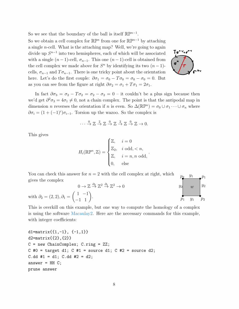
So we see that the boundary of the ball is itself RPn−1.So we obtain a cell complex for RPn from one for RPn−1 by attaching

a single n-cell. What is the attaching map? Well, we’re going to again

divide up Sn−1 into two hemispheres, each of which will be associated

with a single (n− 1)-cell, σn−1. This one (n− 1)-cell is obtained from

the cell complex we made above for Sn by identifying its two (n− 1)-

cells, σn−1 and Tσn−1. There is one tricky point about the orientation

here. Let’s do the first couple: ∂σ1 = σ0 − Tσ0 = σ0 − σ0 = 0. But

as you can see from the figure at right ∂σ2 = σ1 + Tσ1 = 2σ1.

In fact ∂σ3 = σ2 − Tσ2 = σ2 − σ2 = 0 – it couldn’t be a plus sign because then

we’d get ∂2σ3 = 4σ1 6= 0, not a chain complex. The point is that the antipodal map in

dimension n reverses the orientation if n is even. So ∆(RPn) = σ0 ∪ σ1 · · · ∪ σn where

∂σi = (1 + (−1)i)σi−1. Torsion up the wazoo. So the complex is

· · · 0→ Z 2→ Z 0→ Z 2→ Z 0→ Z→ 0.

This gives

Hi(RPn,Z) =

Z, i = 0

Z2, i odd, < n,

Z, i = n, n odd,

0, else

.

You can check this answer for n = 2 with the cell complex at right, which

gives the complex

0→ Z ∂2→ Z2 ∂1→ Z2 → 0

with ∂2 = (2, 2), ∂1 =

(1 −1

−1 1

).

w

y1

y1

y2y2

p2

p1

p1

p2

This is overkill on this example, but one way to compute the homology of a complex

is using the software Macaulay2. Here are the necessary commands for this example,

with integer coefficients:

d1=matrix1,-1, -1,1

d2=matrix2,2

C = new ChainComplex; C.ring = ZZ;

C #0 = target d1; C #1 = source d1; C #2 = source d2;

C.dd #1 = d1; C.dd #2 = d2;

answer = HH C;

prune answer

8

Incidentally, the group manifold of the rotation group SO(3) is RP3.

CPn. Complex projective space CPn is the space of complex lines (copies of C)

through the origin in Cn+1, CPn = ~z/ (~z ∼ λ~z) , λ ∈ C \ 0. We can choose a gauge

where |~z| = 1, leaving just a phase ambiguity: CPn = S2n+1/ (~z ∼ λ~z) , |λ| = 1. To fix

the phase, consider the region where zN+1 6= 0. Then we can use λ to set zN+1 > 0,

so that a general point is of the form ~z = (~w,√

1− |~w|2), |~w|2 ≤ 1. But the set of

points ~w ∈ Cn, |~w|2 ≤ 1 is a B2n. Its boundary occurs when zN+1 = 0, which means

|~w| = 1, which is an S2n−1. On this locus, the phase redundancy still acts. So:

CPn = B2n/(w ∼ λw on ∂B2n = S2n−1) .

Therefore the boundary is a copy of CPn−1. So a cell complex for CPn is ∆(CPn) =

σ0 ∪ σ2 ∪ · · · ∪ σ2n, and the boundary map is just zero. bi(CPn) = 1 for i even and

bi(CPn) = 0 for i odd.

At right is a visualization

of homology which I find

useful.

1.3 Euler-Poincare theorem

The euler character is

χ(X) ≡d∑p=0

(−1)pIp =d∑p=0

(−1)pbp.

Here Ip is simply the number of p-simplices in the triangulation. We’ve seen that this

is sometimes saturated by the minimal cellulation, i.e. no cancellation is required at

all.

Proof: Ip = dim Ωp = dim ker ∂p+dim Im∂p. This is made clear by the visualization

above. Now when we add these up with alternating coefficients, we get the alternating

sum of the betti numbers bp = dim ker ∂p − dim Im∂p+1, using the fact that 0 =

9

dim Im∂d+1. This gives a proof that the euler character is a topological invariant,

independent of the triangulation.

1.4 Exact sequences

Suppose we have a short exact sequence of chain maps:

0→ A•i→ B•

π→ C• → 0.

‘Chain maps’ means that they commute with the boundary operator ∂. ‘Exact se-

quence’ means that the kernel of one map is equal to the image the previous: ker(i) =

0, ker(π) = im(i), im(π) = C. The • just means that we have such a map for each value

of the label.

Such a short-exact sequence on the chains produces a long exact sequence on the

homology:

...∂?→ Hp(A)

i?→ Hp(B)π?→ Hp(C)

∂?→ Hp−1(A)i?→ · · ·

is exact. This involves three statements: exactness at each of the three kinds of nodes.

The only tricky part is the definition of the ‘connecting homomorphism’ ∂?. For more,

see §1.4 of these notes.

2 Cohomology

2.1 de Rham cohomology

[Bott and Tu, early sections, Polchinski §B.4, Nash and Sen §2.3] A p-form on a smooth

manifold M is made from a completely-antisymmetric p-index tensor Ai1···ip

A =1

p!Ai1···ipdx

i1 ∧ · · · ∧ dxip . (2.1)

Here dxi are coordinate differentials, i.e. a basis of cotangent vectors associated with a

set of coordinates onM (dxi(∂xj) = δij)3. The set of p-forms onM (perhaps with some

smoothness and integrability properties) is a vector space Ωp(M). The coefficients can

3In case you are not familiar with these notions, here is brief recap to explain the notation. A

tangent vector on a manifold M at a point p, v ∈ TpM, is of the form v = vi ∂∂xi in terms of some

local coordinates xi. It is a differential operator in the following sense. For any function f and for

any curve xi(t) through p, the rate of change of f along the curve is

df

dt|p =

dxi

dt

∂

∂xif |p.

10

be from any field, but we will think mostly about R. These vector spaces enjoy a

product, the wedge product, which we’ve already written in (2.1). A good way to

define the wedge product is in terms of the coordinate differentials: the wedge product

dxi1 ∧ dxip is completely antisymmetric and separately linear in each factor.

(Ap ∧Bq)i1···ip+q =(p+ q)!

p!q!A[i1···ipBip+1···ip+q ]

where the square brackets indicate antisymmetrization of indices, i.e. average over

permutations weighted by (−1)σ, the sign of the permutation. The wedge product is

graded antisymmetric, meaning

Ap ∧Bq = (−1)pqBq ∧ Ap.

The exterior derivative is a linear differential operator d : Ωp → Ωp+1 defined by

d = dxν ∧ ∂ν , or more explicitly

(dAp)i1···ip+1 = (p+ 1)∂[i1Ai2···ip+1].

It satisfies d2 = 0 by equality of mixed partials: [∂i, ∂j] = 0 on smooth functions.

The main job in life of a p-form on M is to be integrated over p-dimensional

submanifolds Xp ⊂M:∫XpAp is a coordinate-invariant number. Stokes’ theorem says∫

Xp

dAp−1 =

∫∂Xp

Ap−1.

So far, the metric has not been involved. The Hodge star operation requires the

metric:

(?ω)ip+1···in =

√γ

p!εi1···inω

i1···ip .

(Indices are raised using the metric, ωi ≡ gijωj.)

To get some familiarity with the above language let’s think about the caseM = R3

for a moment. Then Ω0(R3) and Ω3(R3) are both spanned by ordinary functions, while

Ω1(R3) and Ω2(R3) are both spanned by vector fields – functions with a single index.

On functions, df = ∂ifdxi. On 1-forms,

d(fidxi) = (∂yfz − ∂zfy) dy∧dz+(∂xfy − ∂yfx) dx∧dy+(∂zfx − ∂xfz) dz∧dx =

1

3!εijk∂ifjεilmdx

l∧dxm.

Since this is true for any dxi

dt = vi and any point p and any f , the important part is the ∂∂xi .

The second ingredient is that a cotangent vector is an element of the dual vector space T ?pM –

an object which eats a tangent vector and gives a number. A basis for such things is given by the

coordinate differentials dxi, which satisfy dxi(∂xj ) = δij .

11

On 2-forms

d(fxdy ∧ dz + fydz ∧ dx+ fzdx ∧ dy) = ∂ifidx ∧ dy ∧ dz.

So this accounts for all the classic operations of vector calculus:

d(0-form) = gradient, d(1-form) = curl, d(2-form) = divergence.

A classical physics context where one encounters a cohomological question is in

fluid dynamics: given a vector field, say describing the flow of a fluid on some space

X, when is it the gradient of a well-defined function on X? Or in electrostatics on

some space X, an allowed electric field configuration must be the gradient of a scalar

potential on X\ the locations of the charges.

The de Rham cohomology H•(X) of a smooth manifold X of dimension n is the

cohomology of the complex

0→ Ω0(X)d→ Ω1(X)

d→ · · · d→ Ωn(X)→ 0.

That is

Hp(X) ≡ ker d : Ωp → Ωp+1

im d : Ωp−1 → Ωp.

It is called cohomology rather than homology because d increases the index p. More

significantly there is some reversal of arrows relative to homology: ‘cohomology is a

contravariant functor’.

There are close relations between homology and cohomology, which come under the

name ‘Poincare duality’. See section 2.5 of these notes for more.

2.2 Cech cohomology

Another, more powerful, cohomology theory is defined as follows.

The simplest version of the idea is to think about locally constant functions on

patches. Locally constant means that on each connected component of its domain, the

function takes a constant value. Cover the manifold X with open sets Uα. These open

sets intersect in e.g. Uαβ ≡ Uα ∩ Uβ, and triple-intersections Uαβγ ≡ Uα ∩ Uβ ∩ Uγ and

so on. Define Ck to be the vector space of A-valued locally-constant functions on the

disjoint union of the (k + 1)-overlaps for some abelian group A:

Ck ≡ locally constant functions,∐

α0···αk

Uα0···αk→ A.

So an element of C0 just assigns an element of A to each Uα. Then there is an analog

of the boundary map (actually coboundary map, since it goes in the other direction)

12

which makes this into a chain complex, δ : Ck → Ck+1. It is defined as a difference

of restrictions, as follows. For example, given f : Uαβ → A on all double-overlaps,

this defines a function f : Uαβγ → A on all triple-overlaps just by restriction. The

coboundary map δ : C0 → C1 is

(δf)αβ = fα − fβ.

The idea is that δf checks agreement, i.e. whether or not f can be regarded as a

function on the union. The map for C1 → C2 is:

(δf)αβγ = fαβ + fβγ + fγα = fαβ + fβγ − fαγ.

Note that we define fαγ ≡ −fγα. There is a similar definition for general k, so that

δ2 = 0, and the cohomology of the complex is well-defined, and again is a topological

invariant (actually the same data as above). The definition for general k is

(δf)α1···αk+1=∑i

(−1)ifα1···αi···αk+1

where α indicates that α is missing. In this expression, we’ve chosen an (arbitrary)

order for the subsets.

Cech cohomology is very simple to actually calculate in rea-

sonable examples. Consider a cover of a circle by three

patches U0, U1, U2, with overlaps U01, U12, U20. The space of

0-cochains is C0 = ωα, α = 0, 1, 2|ωα is constant on Uα =

A3, while the space of 1-cochains is C1 = ηαβ, α, β =

0, 1, 2|ηαβ is constant on Uαβ = A3. There are no triple-

overlaps (and because the space is one-dimensional, there

can be no triple-overlaps in any open cover) so C2 = 0.

U0

U1

U2

U12

U20

U01

S1

The coboundary map δ : C0 → C1 acts by (δω)αβ = ωα − ωβ. The Cech complex is

0→ A3 δ→ A3 → 0

with

δ =

−1 1 0

0 −1 1

1 0 −1

.

More, explicitly H0(S1) = ker (δ) = ω0 = ω1 = ω2 = A. And H1(S1) = A3/im(δ) =

A. A 1-cocycle η = (η01, η12, η20) is a coboundary if η01 + η12 + η20 = 0. So a generator

of H1(S1) is of the form (g, 0, 0) where A = 〈g〉.

13

Not all covers of a manifold will give the same answer. A

good cover is one for which every intersection Uα1···αkis topo-

logically a ball. So the example above is a good cover of the

circle. An example of good cover of the 2-sphere has four

open sets. One is the northern hemisphere. The other three

each cover an enlarged one-third pie-slicing of the southern

hemisphere, as at right.

U0 U1

U2

U01

U20U12

A good cover ofM is associated with a cell decomposition of

M: associated a 0-cell to each open set, if Uαβ is non-empty,

a 1-cell connects the 0-cells α and η. If Uαβγ is non-empty,

we fill in the face of the triangle αβγ with a 2-cell. Keep

going. There is a close relation between δ and the boundary

map for this cell complex. On the homework you can work

out the Cech homology for the 2-sphere and you will see close

parallels with the homology of the tetrahedron.

3 Homotopy

[Hatcher, beginning] First some definitions. A homotopy is a family of maps ft : X →Y, t ∈ I (I is the interval) such that

f :X × I → Y

(x, t) 7→ ft(x)

is continuous. (In the following everything in sight is assumed to be continuous.) Two

maps f0,1 : X → Y are said to be homotopic if there exists a homotopy ft with the

obvious boundary conditions. In this case we will write f0 ' f1.

An important class of examples is the following. A deformation retraction of X

into A ⊂ X is a homotopy from f0 = id : X → X to f1 = a retraction r : X → X

with r(X) = A and r2 = r like a projector. For example, we can find a deforma-

tion retraction of a disk X to a point A, or an annulus X to a circle A, or a disk

with two holes to ∞ or θ or two circles attached by a line segment, like eyeglasses:

14

.

There are retractions which are not deformation retractions, such as from X = two

points to X = one point, or from X = annulus to X = one point.

An important definition: X is homotopy equivalent to Y (or X and Y have the

same homotopy type or X ' Y ) if there exist f : X → Y and g : Y → X such that

f g and g f are homotopic to the identity map.

For example, if X deformation retracts to A ⊂ X via f : X×I → X with r : X → A

the retraction and i : A→ X the inclusion, then ri = 1, and ir ' 1 by the homotopy

f . Therefore X ' A. So the two-hole disk and ∞ and θ and the eyeglasses are all

homotopy equivalent. Another example is Rn and the n-dimensional open ball.

As the name suggests, homotopy equivalence is an equivalence relation, as you can

check. Deformation retraction is not. X ' Y iff there exists Z which deformation

retracts to X or Y . If X ' a point, then we say X is contractible.

3.1 Notions of ‘same’

There are many possible notions of when two spaces are ‘the same’. They differ by

what structure we care about. For example, if we are interested in spaces with metrics,

we regard two spaces to be equivalent if they are related by an invertible isometry –

a smooth map which preserves the metric. If we are just interested in doing calculus,

two smooth manifolds are equivalent if they are related by an invertible smooth map

(diffeomorphism). If we are only doing topology, continuous maps – homeomorphisms

are enough.

Homotopy vs homeomorphism. Homotopy equivalence is yet another notion

of equivalence, which depends only on continuity, but is weaker than homeomorphism.

There are manifolds which are homotopy equivalent but not homeomorphic: a ball and

a point are homotopy equivalent by the deformation retraction, but they have different

dimension. The dimension of a manifold is a homeomorphism invariant, but not a

homotopy invariant.

3.2 Homotopy equivalence and homology/cohomology

If two manifolds are homotopy equivalent, they have the same homology and cohomol-

ogy groups. See section 3.2 and 3.3 of these notes for proofs of these statements.

15

3.3 Homotopy groups

Let X be a topological space with a base point, p ∈ X, just a point in X that we like

for some reason. The homotopy groups of X are:

πq(X) ≡ homotopy classes of maps : (Iq, ∂Iq)→ (X, p).

Here Iq ≡ I × I × · · · I is the inside of the q-dimensional cube, homotopic to a q-ball,

and its boundary is the unit cube, homotopic to a (q − 1)-sphere. Since all points in

∂Iq map to the same point in X, an equivalent definition would consider maps from

Iq/∂Iq ' Sq taking the north pole to the base point.

For q > 0, πq is a group under the following product operation: Given α, β :

(Iq, ∂Iq) → (X, p) (so that [α], [β] ∈ πq(X)), define [α][β] = [α ? β] where α ? β is the

map

(α ? β)(t1, · · · , tq) =

α(2t1, t2, · · · , tq) , 0 ≤ t1 ≤ 1

2

β(2t1 − 1, t2, · · · , tq) , 12≤ t1 ≤ 1

α β

t1

t2

(3.1)

(I draw the picture for q = 2. All the black lines map to the base point.)

If instead we were using maps from Sq, we first

map Sq to two Sqs attached at their north poles

by shrinking the equator to a point, then map the

top sphere by α and the bottom sphere by β.

For q = 0, π0(X) = maps : point → X/ '≡ [point, X] is not in general a group.

Rather π0(X) is the set of path components of X. (For the special case where X = G

is a Lie group, π0(G) = G/G0, where G0 is the component of G containing the identity

element; this is a group.)

Basic facts about homotopy groups:

1. πq(X) is a group. The identity operation is the constant map to the base point.

The inverse is [f−1(t1 · · · tq)] = [f(1− t1, t2, · · · tq)].

16

The product is associative in the sense that

α∗ (β ∗γ) ' (α∗β)∗γ are homotopy equiv-

alent. Here is the homotopy:

α β γ

1/4 1/2

1/2 3/4

(α ∗ β) ∗ γ

α ∗ (β ∗ γ)

t

s

2. πq(X) is abelian for q > 1. π1(X), called the fundamental group of X, is special

in that it can be non-abelian.

Proof of statement 2:

α β 'α

βp

p'

α

β

'β p

p ααβ'

α ? β δ

α ? β in the first step is the map in (3.1). Here the definition of the map δ:

δ(t1, · · · , tq) =

α(2t1, 2t2 − 1, · · · , tq) , 0 ≤ t1 ≤ 1

2, 12≤ t2 ≤ 1

β(2t1 − 1, 2t2, · · · , tq) , 12≤ t1 ≤ 1, 0 ≤ t2 ≤ 1

2

p, otherwise

– the points in the lower left and upper right all map to the base point.

3. If X ' Y then πq(X) ∼= πq(Y ).

4. πq(X × Y ) = πq(X)× πq(Y ). Even simpler than the Kunneth formula.

Basic fact 4 follows from the fact that any map Iq → X × Y is of the form

(fx, fy) with fx : Iq → X, fy : Iq → Y . And it is a group homomorphism since

(fx, fy) ? (gx, gy) = (fx ? gx, fy ? gy).

5. Let ΩpX ≡ continuous maps : (I1, ∂I1)→ (X, p) ≡ the loop space of X. So the

definition of π1(X, p) is just π0(Ωp(X)). For q > 2 also4, πq−1(ΩpX) = πq(X, p).

4This is a teleological footnote using ideas we’ll develop below to prove this statement more. Please

ignore it on a first pass. I learned it from Bott and Tu and here. The following sequence (for X path

connected) defines a fiber bundle

ΩX → PX → X (3.2)

called the path fibration where PX ≡ maps µ : I → X,µ(0) = p (p is the base point). The first

17

The idea is that a representative of πq(X), f : Iq → X can be viewed instead as

a map Iq−1 → ΩX just by picking a slice of Iq.

A corollary of this statement is that π1(ΩX) is always abelian.

6. Like homology, πq is a covariant functor from the category of topological spaces

(and continuous maps) to the category of groups (and group homomorphisms).

To see this, consider a map φ : (X, x0) → (Y, y0). Given a representative of

πq(X), α : (Iq, ∂Iq) → (X, x0), we can use φ to make a representative of πq(Y ),

namely φ f : (Iq, ∂Iq) → (Y, y0). So we can define an induced map on the

homotopy groups

φ?[α] ≡ [φ f ].

This is a group homomorphism in the sense that 1? = 1, φ(α?β) = (φα)?(φβ)

and given also ψ : (Y, y0)→ (Z, z0), we have ψ? φ? = (ψ φ)?.

One consequence of this is the obvious-sounding statement (basic fact 3) that

homotopy-equivalent spaces have the same homotopy groups (Hatcher Proposi-

tion 1.18). If f : X → Y and g : Y → X are the relevant maps then the induced

map f? : πq(X, x0)→ πq(X, f(x0)) is an isomorphism with inverse g?.

7. Making the choice of base point explicit, πq(X, p) ∼= πq(X, p′) (i.e. they are

isomorphic groups) if X is path connected. So we don’t need to make the choice

of base point explicit.

About the dependence on the base point (item 7): Suppose

that X is path connected. A path γ from x0 to x1 induces a

map on the loop spaces Ωx0X → Ωx1X by α → γ ? α ? γ−1

(where γ−1 means the path γ traversed backwards).γ

γ−1

x0 x1

α

This induces a map

γ? : πq−1(Ωx0X, x0)→ πq−1(Ωx1X, x1)

map is just inclusion (ΩX = µ ∈ PX|µ(1) = p), and the second map is the projection π(µ) = µ(1).

The statement that (3.2) is a fiber bundle means the second map in (3.2) satisfies the ‘homotopy

lifting property’ or ‘covering homotopy property’ (this elaborate-seeming statement is explained on

page 198-199 of Bott and Tu; the fact that it holds for π : PX → X is simple when X is path-

connected). This means the short-exact sequence (3.2) induces a long-exact sequence on the homotopy

groups

· · · → πq(ΩX)→ πq(PX)→ πq(X)→ πq−1(ΩX)→ · · ·

And finally PX is contractible because each path can be deformation retracted to the base point,

or as it says in the link above: ”the picture is that of sucking spaghetti into one’s mouth?.

So the exactness of the long-exact sequence means πq(X) ∼= πq−1(ΩX).

18

where xt is the constant map to xt. But this is the same as a map

γ? : πq(X, x0)→ πq(X, x1).

This map is an isomorphism, with (γ−1)? = (γ?)−1.

More explicitly, for [α] ∈ πq(X, x0) define a homotopy

F : Iq+1 = Iq × I → X

as follows. For u ∈ Iq, we want F (u, 0) = α(u) and F (u, t) =

γ(t),∀u ∈ ∂Iq. This defines the map on all but one face of ∂Iq+1.

Now I quote a theorem (‘the box principle of obstruction theory’)

that such an F can be extended to all of Iq+1, and we define

[F (u, 1)] = γ?[α].

x0 x0

x0x0

x1

x1

x1

x1

α

γγ

γ

If we take x0 = x1, this defines an action of π1(X, x0) on πq(X, x0) describing the

result of moving the base point around in a non-contractible loop. Its nontriviality

measures something about how much the choice of base point matters. Bott and Tu

Prop. 17.6.1 shows that

πq(X, x0)/π1(X, x0) ∼= [Sq, X]

where the quotient on the LHS is by the action defined above, and the RHS is homotopy

classes of maps from Sq to X without any notion of base point (‘free homotopy’). This

is not a group. The map from the LHS to the RHS is just inclusion of base-point-

preserving maps into the set of all maps.

What’s special about Iq or spheres? It is actually possible to define homotopy

groups of maps from other spaces. But in general the set of homotopy classes of maps

from one space to another is not a group.

Higher homotopy groups are hard to compute. Even for spheres πq(Sn) are not all

19

known for large-enough q and n. For small q, n here is the table:

(from here; that page also has a larger table).

Fundamental group. Let’s focus on q = 1, the fundamental group, for a bit.

In this case the product is simpler to understand: a representative of π1(X) is just a

closed path in X starting and ending at the base point. The product of two paths is

just one followed by the other, with the parameter rescaled so that total duration is

still 1.

There is information in πq(X) that is not present in the homology. For example,

π1(X) has more information than H1(X). Here is an example of a space X with trivial

H1(X,Z) (such a space is called ‘acyclic’) but nontrivial π1(X). Take a figure eight

and glue in two 2-cells whose boundaries are a5b−3 and b3(ab)−2 where a and b are the

two loops. The cell complex is then

0→ Z2 M→ Z2 0→ Z→ 0

with

∂2 = M =

(5 −2

−3 1

). Since detM = −1

there is not even any torsion first homology. But

π1(X) =⟨a, b|a5b−3 = 1, b3(ab)−2 = 1

⟩=⟨a, b|a5 = b3 = (ab)2

⟩= I? (3.3)

the binary icosahedral group, a double cover of the icosahedral group (the symmetry

group of the icosahedron and dodecahedron) I ∼= A5, also known as the alternating

group on (i.e. the even permutations of) five elements, S5/Z2. Under the surjection

I?→ I a maps to a 2π/5 rotation through center of a pentagon, and b maps to a 2π/3

20

rotation through a vertex. The double cover of I arises by the inclusion I ⊂ SO(3),

and is induced by the double cover π : SU(2)→ SO(3).

Why is (3.3) the answer for π1(X)? Well, π1 of a bouquet of circles – q circles

attached at a point (which we take to be the base point) – is the free group on q elements.

Each circle provides a generator, and there are no relations. A bouquet of q circles is a

deformation retract of R2 \ q points (or R3 \ q lines), ' , so this

is also π1 of the latter spaces.

This free group on ≥ 2 elements is a deeply horrible object. The elements are all

words made of the letters a1, a2 · · · aq and a−11 , a−12 · · · a−1q , and the only relation is that

you can cancel an ai and an a−1i if they are right next to each other. It contains copies

of itself as a subgroup. Ick.

When we glue in a 2-cell we introduce a relation in π1 according to the gluing map;

this gives (3.3).

This example is related to the existence of the Milnor homology sphere M – a

3-manifold with the same homology as a sphere, but different homotopy groups. M

can be defined as S3/I? (with I? the binary icosahedral group as above). Therefore

π1(M) = I ′. There is a lot to say about this space.

General Fact: H1(X,Z) is the abelianization of π1(X), i.e.

H1(X,Z) = π1(X)/[π1(X), π1(X)]

where [G,G] ≡ 〈ghg−1h−1, g, h ∈ G〉 is the commutator subgroup of G, the subgroup

generated by (multiplicative) commutators of elements of G. This is not hard to see:

the whole difference between π1 and H1 is that in the latter we keep track of the order

in which the closed loops are traversed. Modding out by commutators is erasing exactly

this information. [For a more explicit proof, see Hatcher Theorem 2A.1.]

van Kampen Theorem. [Justin Roberts’ knot knotes has a very nice discussion

with a proof sketch] Here is a way to compute the fundamental group of a space by

chopping up the space. Let X = U ∪ V , two open sets, and let W ≡ U ∩ V . Denote

π1(Y ) ≡ 〈sY |rY 〉 for Y = U, V,W , so sY is a set of generators of π1(Y ) and rY is a set

of relations. Let iU,V be the inclusion maps of W into U and V . Then

π1(X) =⟨sU ∪ sV |rU ∪ rV ∪ iU? (g) = iV? (g)g∈sW

⟩.

That is: a set of generators of π1(X) is just those of U and those of V . This double-

counts the generators on the overlap. The theorem says that it’s enough to add one

relation for each generator of the fundamental group of the overlap.

21

Example 1: Cut a bouquet of two circles (S1∧S1, two circles

attached at a point) into two open sets U and V where each

of U and V removes a single point from one of the circles.

The overlap can be deformed to an X which is contractible.

π1(U) and π1(V ) each have one generator, and there are no

relations, so π1(S1 ∧ S1) is the free group on two elements.

Example 2: Consider a genus-g Riemann surface Σg, de-

scribed as a polygon with 2g sides, with the identifications

given in §1.2. Let U be a disk inside the polygon and V a

little more than its complement. Then U ∩ V is an annulus,

homotopy equivalent to a circle, with π1(S1) = 〈g〉 . The

inclusion of g into U maps it to iU? (g) = 0, since every loop

in U is trivial. The inclusion of g into V is homotopic (in

V ) to∏g

i=1[ai, bi] with [a, b] ≡ aba−1b−1. We conclude that

π1(Σg) = 〈ai, bigi=1|∏g

i=1[ai, bi]〉.

Example 3: The answer we found above for π1 of the acyclic space X can also be

obtained by these methods. It is best to do it in two steps, first removing both disks

and then removing just one.

Higher homotopy groups and homology. For general q, there is a natural

homomorphism

i :πq(X) → Hq(X)

[f ] 7→ f?(u)

where u is a generator of Hq(Sq). For better or worse, this map is neither injective nor

surjective.

One more fact about the relation between homotopy groups and homology, however,

is the Hurewicz isomorphism theorem: The first nontrivial homotopy and homology

groups of a path-connected manifold occur in the same dimension q. (q = 0 doesn’t

count.) If q > 1 then they are isomorphic. (In symbols: if q > 1, and πk(X) = 0 for

1 ≤ k < q, then Hq(X) = 0 for 1 ≤ k < q and Hq(X) = πq(X).)

Consider the case q = 2. Then the claim is that H2(X)·

= H1(ΩX) = π1(ΩX)

(since π1(ΩX) = π2(X) is abelian), and therefore H2(X) = π2(X). The first equality,

with the·

=, follows from H1(X) = 0 but I will not explain it here. There is a general

proof on page 225 of Bott and Tu which uses a spectral sequence and induction from

the above case.

This theorem implies that πq(Sn) = δn,qZ for q ≤ n.

22

3.4 Fiber bundles and covering maps

When does an ‘exact sequence of spaces’ like

0→ Fi→ E

π→ B → 0 (3.4)

induce a long exact sequence on their homotopy groups

· · · → πq(F )i?→ πq(E)

π?→ πq(B)∂→ πq−1(F )→ · · · → π1(B)

∂→ π0(F )i?→ π0(E)

π?→ π0(B)→ 0

(3.5)

? In general it does not. But with some extra assumptions on the sequence of contin-

uous maps (3.4) it does. The extra assumption says that E is a fiber bundle; B is the

base, and F = π−1(b0) is the fiber. I mention this here also because this notion will

play an important role in the interpretation of the quantum double model.

Part of the assumption is that a neighborhood every fiber π−1(U) is homeomorphic

to U × F . Such a map π is called a covering map.

The further condition for E to be a fiber bundle is that for each

open set Uα in a cover of B, the diagram at right commutes. The

vertical map is just forgetting about the fiber.

π−1(Uα) Uα × F

Uα

φ

π

These maps φα : π−1(Uα) → Uα × F are then called local trivializations, analogous to

local coordinates on a manifold. For the pathologists among you: try to come up with

an example of a covering map which does not produce a fiber bundle; I don’t want to

do it.

A section of a fiber bundle is a map s : B → F with π s = 1.

Transition functions. Now on the double-overlaps Uαβ of an open cover of B, we

have maps

φα φ−1β : Uαβ × F → Uαβ × F.

These are called transition functions. They lie in a subgroup of the group of homeo-

morphisms of the fiber F called the structure group of the bundle.

Of course a product manifold, like T 2 = S1×S1, is a fiber bundle, but a trivial one,

where the transition functions can all be chosen to be the identity. (If we were keeping

track of more information, such as the complex structure on the torus, the boundary

conditions which identify S1 with S1 by a shift gives a nontrivial operation called a

Dehn twist.)

23

Example: Mobius band. Take B = S1 and

F = I. If we impose boundary conditions that the

orientation of F reverses when we go around the cir-

cle, we get the Mobius band.

Cover B = S1 with two open sets U1,2. They over-

lap in U12 = A ∪ B, with two components. The

nontrivial transition functions are

φ12(x) =

1 if x ∈ Ag if x ∈ B

where g is the orientation-reversal of the fiber. B = S1

F = I

A very similar example is obtained by replacing the fiber by S1; this is the Klein

bottle.Example: Hopf bundle. Take E = the unit quaternions,

or SU(2) ' S3, and F = S1, the unit complex numbers inside

the unit quaternions. Taking S3 ⊂ C2 = (z0, z1), the base

is (S3 = |z0|2 + |z1|2 = 1 ⊂ C2

)/(z0, z1) ∼ eiα(z0, z1)

which is CP1 ' S2. This is just the Bloch sphere of normal-

ized pure states of a qubit, and the projection map is just

forgetting the overall phase of the wavefunction. In stere-

ographic projection S2 ' C ∪ ∞, the projection map is

π : (z0, z1) → z0/z1, where the range of the map is B ' S2

is the Riemann sphere (complex plane union the point at in-

finity). In polar coordinates (r20 + r21 = 1 defines the S3) the

projection is π(r0eiθ0 , r1e

iθ1) = r0r1ei(θ0−θ1). Fixed ρ = r0/r1

is a T 2 ⊂ S3 which degenerates at ρ = ±∞ to two linked

circles. A visualization from Wikipedia is at right.

Another way to present the Hopf bundle projection, which arises all the time in

physics is:

π :

C2 → R3

S3 → S2

z 7→ z†~σz

The top row applies to general z = (z0, z1), and the middle row applies to the subspace

where |z0|2 + |z1|2 = 1. We can make local sections of this bundle by finding the ±1

eigenvectors of n · ~σ.

24

One reason to care about the Hopf bundle, besides its ubiquity in theoretical physics,

is that it gives relations between homotopy groups of spheres. The exact homotopy

sequence is

· · · πq(S1)→ πq(S3)→ πq−1(S

2)→ πq−1(S1)→ · · · (3.6)

Fact: πq(S1) = Zδq,1 for q ≥ 1. We conclude from (3.6) that πq(S

3) ∼= πq(S2) for

q ≥ 3. In particular π3(S2) = Z is generated by the Hopf projection itself.

Universal cover. How do we know the homotopy groups of the circle? One way

is to write S1 = R/Z. Now we appeal to the following

General Fact: if X = C/G and C is simply connected (≡ π(C) = 0) then π1(X) = G.

(If you are not happy with this level of detail, Hatcher has a long section on π1(S1).)

Of intermediate generality between a quotient and a fiber bundle is the existence of

a covering map π : C → X. If C is simply connected, then the space C is called the

universal cover of X. For example, we saw in §1.2 that a Riemann surface Σg of genus

g ≥ 1 can be made by taking a disk and making identifications along its boundary.

Since the disk is simply connected, it is the universal cover of Σg, and

π1(Σg) =⟨ai, bi|a−11 b−11 a1b1a

−12 b−12 a2b2 · · · a−1g b−1g agbg = 1

⟩where the one relation comes from the disk filling in the boundary. (By this notation I

mean the group generated by the list of things before the |, modulo the list of relations

after the |.) For g = 1, this says that a and b commute, which they’d better since

π1(T2) = π1(S

1) × π1(S1) = Z × Z is abelian. For g > 1, π1(Σg) is non-abelian. You

can see that its abelianization is Z2g in agreement with our previous result for H1(Σg).

Brief and insufficient words about the connecting homomorphism. [Bott

and Tu p. 209] I said that for fiber bundles there is a long exact sequence on the

homotopy groups, but what is the mysterious map ∂ : πq(B)→ πq−1(F ) in (3.5)?

The idea is that a map α : Iq → B can be lifted to a

map α : Iq → E, but it does not necessarily end at the

base point of E, since the base point of B can have many

pre-images in E, only one of which is the base point in

E. Regard F = π−1(b0) as the fiber over the base point.

First the case q = 1: the lift of α can be chosen so that

α(0) is the base point in F . Then ∂[α] = [α(1)].

For general q, the properties of a fiber bundle guarantee that α can be lifted so that

α(t1, · · · tq−1, 0) lifts to the constant map to the base point of F . Then its image under

25

the connecting homomorphism is

∂[α] = [(t1 · · · tq−1) 7→ α(t1 · · · tq−1, 1)].

α in the same homotopy class have the same image. The keyword is ‘covering homotopy

property’.

One final comment about covering maps: If π : (X, x0) → (X, x0) is a covering

map, then π? : πq(X, x0) → πq(X, x0) is an isomorphism for q ≥ 2. The idea is that

every map Sn → X lifts to a map Sn → X for q ≥ 2. This is Hatcher Prop. 4.1 on page

342, and also follows from the ‘covering homotopy property’. In the case of q = 1, the

induced map is merely injective, and embeds π1 of the covering space as a subgroup

of π1(X) (Hatcher Prop. 1.31) – it’s just the subgroup of loops which lift to closed

loops in X (unlike the one α in the figure above). There is therefore a correspondence

between covers of X and subgroups of π1(X).

3.5 Relative homotopy.

It is possible define a notion of relative homotopy. Given Y ⊂ X a closed subspace

containing the base point p, the relative homotopy group is

πq(X, Y, p) ≡ πq−1 (paths from p to Y )

or slightly more explicitly

πq(X, Y, p) = α : (Iq, ∂Iq)→ (X, p or Y )/ ' . (3.7)

What I mean by this is: all of the faces of ∂Iq get mapped to the base point as usual,

except for the bottom face of ∂Iq, which gets mapped anywhere into Y . By the ‘bottom

face’ of ∂Iq I mean t1 = 0. So α|t1=0 : (Iq−1, ∂Iq−1)→ (Y, p). The product is defined

as usual for q > 1, but π1(X, Y ) is not a group.

The inclusion map i : Y → X induces a map i? : πk(Y, p) → πk(X, p) as usual.

Noting that πk(X, p) = πk(X, p, p), we also have a map

j? : πk(X, p) = πk(X, p, p)→ πk(X, Y, p).

Finally, we can define

∂? :πk(X, Y, p) → πk−1(Y, p)

α 7→ α|bottom face.

This produces a long exact sequence on homotopy:

· · · → πk(Y, p)i?→ πk(X, p)

j?→ πk(X, Y, p)∂?→ πk−1(Y, p)

i?→ · · · .

Nash and Sen (page 117) use this sequence to show πq(Sn) = 0 for q < n. I must

admit, though, that I do not understand what they mean by B ⊃ Sn.

26