Physics 7230: Statistical Mechanics

Lecture set 5: Density Matrix

Leo Radzihovsky∗

Department of Physics, University of Colorado, Boulder, CO 80309

(Dated: February 24, 2021)

Abstract

In this set of lectures, we will introduce and discuss the properties and utility of the density

matrix - a special quantum mechanical operator whose diagonal elements give the probability dis-

tribution for quantum mechanical microstates. It is a generalizaiton of convention wavefunction

formulation of quantum mechanics, and in equilibrium allows computation of the partition func-

tion and therefore thermodynamics in quantum statistical mechanics. We will also discuss how

thermodynamics (ETH) and in particular entropy – the so-called “entanglement” entropy – arises

in a closed quantum system from entanglement of a subsystem with the rest of the system.

∗Electronic address: radzihov@colorado.edu

1

I. DENSITY MATRIX FUNDAMENTALS IN QUANTUM STATISTICAL ME-

CHANICS

A. General basics

Density matrix ρ was first introduced by John von Neumann in 1927 and independently

by Lev Landau, and as we will see supercedes conventional wavefunction formulation of

quantum mechanics.

Given a density matrix characterizing a statistical ensemble of a quantum system and

obeying normalizaton conditions,

Tr[ρ] = 1, Tr[ρ2] ≤ 1, (1)

the averages of any operator O can be computed according to,

〈O〉 = Tr[Oρ]. (2)

A density matrix is given by a statistical state of a quantum system. Much as a wave-

function, once prepared in an initial state evolves in time according to the time dependent

Schrodinger equation (or equivalently according to the evolution operator U(t) = e−iHt/~,

|ψ(t)〉 = U(t)|ψ(0)〉), subject to systems Hamiltonian H, a density matrix evolves according

to the von Neumann equation (also known as the Liouville - von Neumann equation),

i~∂tρ = [H, ρ], (3)

or equivalently, ρ(t) = U(t)ρ(0)U †(t) (not to be confused with the Heisenberg equation for

evolution an operator, which has an opposite sign).

The von Neumann entropy

SvN = −Tr [ρ ln ρ] = −〈ln ρ〉 = −∑n

λn lnλn, (4)

where λn are eigenvalues of ρ is the quantum mechanical counter-part (generalization) of

the Shannon’s entropy SS = −∑

q Pq lnPq = −〈lnPq〉.

2

B. Equilibrium density matrix

For a system in thermal equilibrium the density matrix is must be stationary and is

thus, according to (3) is taken to be a function of the Hamiltonian, with a form special to

ensembles discussed in Lectures 2-4,

• Microcanonical

ρmc =1

Ωδ(E − H) (5)

• Canonical

ρc =1

Ze−H/kBT (6)

• Grandcanonical

ρgc =1

Ze−(H−µN)/kBT (7)

Detailed balance of transitions between different states required to atain statistical equi-

librium demands that ρ is a Hermitian operator.

Focusing on the canonical (equally true for grandcanonical) ensemble, we note that the

unnormalized part of density matrix ρuc (β) = e−H/kBT satisfies a useful operator differential

equation,

∂β ρuc = −Hρuc (β), (8)

that can be verified by formal substitution, utilizing a Taylor series in H representation

of ρuc (β). One can view this as a time-dependent Schrodinger equation in an imaginary

time, τ = it (where τ ranges from 0 to β~). Equivalently, when expressed in coordinate

representation (see below) one can also view this as an equation in real time for diffusion in

a potential.

II. PURE STATES IN QUANTUM MECHANICS

Recall from standard quantum mechanics, that states |ψ〉 of an isolated quantum sys-

tem are rays (since normalization creates physical equivalence class) in Hilbert space with

expectation values of physical observables, represented by Hermitian operators O are given

by,

〈O〉 = 〈ψ|O|ψ〉.

3

A. Dirac basis-independent representation

It is convenient to introduce a completely equivalent description in terms of the so-called

“pure” density matrix

ρ = |ψ〉〈ψ|, (9)

in terms of which we have,

〈O〉 = 〈ψ|O|ψ〉 = Tr[Oρ], (10)

as given in (2).

One advantage of using ρ over states |ψ〉 is that the overall unphysical phase disappears,

so in a sense density matrix is more physical.

Using time-dependent Schrodinger equation for |ψ(t)〉 we obtaint the von Neumann

equation for the evolution of ρ(t). We can also check that

Tr[ρ] = 1, Tr[ρ2] = 1, (11)

and is a defining property of a pure density matrix state, i.e., a density matrix that corre-

sponds to a single quantum mechanical state |ψ〉, which of course can be a superposition of

many other states. This is to be contrasted with the “mixed” density matrix, to be discussed

in next subsection.

B. Basis representation

Just like a state |ψ〉 =∑

n cn|n〉 can be represented in terms of a orthonormal basis as

a state vector cn, so can density matrix can be represented as a basis-dependent matrix

ρnm, where

ρ =∑n,m

ρnm|n〉〈m| (12)

with matrix elements by definition given by ρnm = 〈n|ρ|m〉 = cnc∗m.

In terms of this representation the trace in (10) is easily computed, giving

〈O〉 = Tr[Oρ] =∑nm

Onmρmn (13)

4

The time evolution is given by matrix version of (3) for Hnm and ρnm. It is convenient

to choose |n〉 to be eigenstates of H, such that H|n〉 = En|n〉, which then gives,

ρnm(t) = ρnm(0)e−i(En−Em)t/~, (14)

consistent with above ρnm = cnc∗m representation and showing that diagonal matrix elements

of ρ are stationary in the Hamiltonian basis and the off-diagonal coherences oscillate at

frequency set by the difference of energy eigenvalues.

The property (11) is just a reflection of the normalization of |ψ〉 that pure ρ is describing.

We also note that a pure density matrix, ρ in (9) can be viewed, somewhat perversely in the

basis of |ψ〉 itself. It is then a matrix of all zeros (corresponding to all other states transverse

to |ψ〉 and 1 as ρψψ = 〈ψ|ρ|ψ〉 = 1. From this extremely degenerate, rank 1 matrix many of

the above expressions e.g., (11) become obvious.

We next consider a generalization of conventional quantum mechanics to that describing

a statistical ensemble of quantum states. Such system is described by a “mixed” density

matrix, to be discussed in next subsection.

III. MIXED STATES IN QUANTUM MECHANICS

We now generalize above analysis to “mixed” density matrix that describes a statistical

ensemble of pure quantum states, that cannot be represented as any state ψ〉. As such,

mixed density matrix is not equivalent to conventional states of a single quantum mechanical

system.

A. General

Thus we consider a “mixed” density matrix, defined as an ensemble of pure density

matrix with probability pi,

ρ =∑i

pi|ψi〉〈ψi|, (15)

5

with normalization∑

i pi = 1, in terms of which we have,

〈O〉 =∑i

pi〈ψi|O|ψi〉 = Tr[Oρ], (16)

where there is both a quantum mechanical and statistical averages.

We can also check that

Tr[ρ] = 1,Tr[ρ2] ≤ 1, (17)

with the second equation being the litmus test for a density matrix describing a mixed state.

It can be traced to the fact that p2i ≤ 1.

B. Thermal equilibrium

In thermal equilibrium ρ(H) take on the form (5)-(7) in the first section, above, with

specific form depending on the ensemble. All other properties of mixed density matrix goes

through. As an example we focus on the canonical ensemble.

1. Hamiltonian eigenstates representaton

As discussed above ρ is a Hermitian operator, generically represented by a corresponding

matrix ρnm = 〈n|ρ|m〉. In the special basis of the Hamiltonian eigenstates, the density matrix

simplifies significantly,

ρ =1

Z

∑n

e−En/kBT |n〉〈n|

taking a diagonal form,

pn =1

Ze−En/kBT , ρnm =

1

Ze−En/kBT δnm = pnδnm,

that is quite convenient for many equilibrium computations and makes the quantum statis-

tical mechanics closer to the classical one.

6

2. Position representaton

Another useful and important basis is the position/coordinate basis, |x〉 that are eigen-

states x|x〉 = x|x〉 of the position operator x, with eigenvalue x. The canonical ensemble

unnormalized density matrix in this representation is given by,

ρu(x, x′; β) = 〈x|e−βH |x′〉 =∑nm

〈x|n〉〈n|e−βH |m〉〈m|x′〉, (18)

=∑n

ψn(x)ψ∗n(x′)e−βEn , (19)

expressed purely in terms of the Hamiltonian eigenfunctions and eigenvalues. We note the

close relation of ρu(x, x′; β) to the evolution operator in quantum mechanics U(x, x′; t),

identifying the former as the evolution operator in imaginary time t = −iτ = −iβ~ (note

the units are indeed that of time), converting (i.e., analytically continuing) U(t) = e−iHt/~

to ρu(β) = e−Hτ/~, with ρu(β) = U(−iβ~).

Recalling an operator differential equation satisfied by equilibrium (canonical) density

matrix, Eq.(8), in coordinate representation it takes the form,

∂βρu(x, x′, β) = −H(p, x)ρu(x, x′, β), (20)

where p = −i~∂x, i.e., giving the coordinate representation Schrodinger equaiton in imagi-

nary time.

Thinking about the fundamental definition of ρu in (6), (7) or equivalently the evolution

equation (20), we also note that ρu(x, x′, τ) satisfies an important “propagator” property,

ρu(x2, x0; τ1 + τ2) =

∫dx1ρ

u(x2, x1; τ2)ρu(x1, x0; τ1), (21)

in analogy with a quantum mechanical propagator.

The corresponding expectation value of an operator O is given in coordinate space

〈O〉 =

∫dxdx′O(x, x′)ρ(x′, x), (22)

an extension of the general result (13) to coordinate representation.

7

3. Path-integral representation

As discussed in earlier lectures, Hamiltonian approach to computation of thermodynamic

averages for quantum systems requires (in comparison to classical statistical mechanics) an

additional step of a diagonalization of the Hamiltonian to obtain En. We mention here

for completeness that an alternative approach invented by Richard Feynman[14, 15], allows

one to bipass the diagonalization step, but at the cost of working with a path-integral over

(imaginary) time-dependent microscopic degrees of freedom qn(τ), with an exponential

of the corresponding Euclidean classical action (obtained from standard action by replacing

t = −iτ), SE[qn(τ)] =∫ β~

0dτL[qn(τ)] as the counter-part of the Boltzmann weight, with

L[qn(τ)] the classical Lagrangian. This is not surprizing, given the connection we have

already seen in Eq.(20). Namely, for a quantum system the coordinate-space density matrix

can be written as partition function can be written as a path-integral[15],

ρu(x, x′; β) =

∫x(0)=x,x(β~)=x′

[dx(τ)]e−SE [x(τ)]/~, (23)

and the associated partition function is the trace,

Z =∑qn(τ)

e−SE [qn(τ)]/~, (24)

=

∫dxρu(x, x; β), (25)

=

∫ ∞−∞

dx

∫x(0)=x,x(β~)=x

[dx(τ)]e−SE [x(τ)]/~, (26)

where the imaginary time ranges over a finite interval, 0 ≤ τ ≤ β~, with periodic boundary

conditions x(0) = x(β~).

This thereby reduces quantum statistical mechanics of a point (0d) particle described

by q ≡ x, (i.e., zero-dimensional “field”) to a classical statistical mechanics of a fluctuating

closed “curve” - “polymer string”, described by a 1d closed curve q(τ) with the effective

classical Hamiltonian given by

Heff [q(τ)] ≡ SE[q(τ)]/~.

8

In passing we note that this nicely extends to quantum field theory of a d-dimensional system

with field operators φ(x) to a d + 1-dimensional path-integral formulation over commuting

field degrees of freedom, φ(x, τ), whose description can be viewed as an effective classical

statistical field theory over fields φ(x, τ).

We also note that in the limit of high temperature (much higher than any natural

frequencies of the system), q(τ) are τ independent and the Euclidean action reduces to

1~

∫ β~0dτL[q(τ)]→ βH(q), and the partition function reduces to the classical one.

We note that the above path-integral representation of d-dimensional quantum statistical

mechanics in terms of (d+1)-dimensional classical statistical mechanics is a direct imaginary

time analog of Feynman’s representation of the Schrodinger quantum mechanics, |ψ(t)〉 =

U(t)|ψ(0)〉 written in terms of the evolution operator U(t) = e−iHt/~ in terms of the path-

integral in real time[14], where in coordinate representation it is given by, U(x, x′;T ) =∫x(0)=x,x(T )=x′

[dx(t)]eiS[x(t)]/~.

IV. DENSITY MATRIX EXAMPLES

We will now present a few sample density matrices in various representations and exam-

ine their properties.

Given a state |ψ〉 we can always construct a pure density matrix as described above.

A mixed density matrix depends on the statistical ensemble characterized by probability

distribution pi can also be constructed for any specific situation. In equilibrium the density

matrix is completely determined by the Hamiltonian of the system, given by Eqs.5,6,7, with

the corresponding E, T , µ, depending on the ensemble of choice.

A. Spin-1/2 states

• Pure state |+, n〉 of spin 1/2 polarized along n = (sin θ cosφ, sin θ sinφ, cos θ):

Such state can be written in the | ↑〉, | ↓〉 basis, the eigenstates of Sz, |+, n〉 =

cos θ2e−iφ/2| ↑〉+ sin θ

2eiφ/2| ↓〉.

9

The corresponding pure density matrix is given by

ρpure,n = |+〉〈+| = cos2 θ

2| ↑〉〈↑ |+ sin2 θ

2| ↓〉〈↓ |+ cos

θ

2sin

θ

2e−iφ| ↑〉〈↓ |+ cos

θ

2sin

θ

2eiφ| ↓〉〈↑ |,

(27)

that has matrix elements given by

ρpure,nσ,σ′ =

cos2 θ2

cos θ2

sin θ2e−iφ

cos θ2

sin θ2eiφ sin2 θ

2

. (28)

In the |+, n〉, |−, n〉 basis its matrix elements are given by,

ρpure,nσ,σ′ =

1 0

0 0

. (29)

In the case of photons such pure state describes perfectly polarized light. This density

matrix can be straightforwardly demonstrated to satisfy normalization, Tr[ρ] = 1,

purity condition Tr[ρ2] = 1, and gives ~/2 for the expectation values of n · ~S. For

θ = π/2, φ = 0, we find 0 for Sz and ~/2 for Sx.

For latter choice of quantization axis, θ = π/2, φ = 0, it is an eigenstate of Sx, and

reduces to,

ρpure,x =1

2(|0〉+ |1〉) (〈0|+ 〈1|) , (30)

=1

2(|0〉〈0|+ |1〉〈0|+ |0〉〈1|+ |1〉〈1|) . (31)

with the matrix representation given by

ρA =1

2

1 1

1 1

, (32)

and we used another common notaton of |0〉, |1〉 basis (used in quantum information),

isomorphic to up/down spin basis.

• Mixed state at infinite temperature:

10

If instead we consider an ensemble state that is an equal statistical mixture of all

quantization axes, n uniformly distributed over 4π steradians (for photons we would

call this “unpolarized” light from eg., an incandescent light bulb), the density matrix

is given by,

ρmixedσ,σ′ =

1/2 0

0 1/2

, (33)

which can be straighforwardly obtained by averaging ρpure,nσ,σ′ (θ, φ) over n on a surface of

Stokes sphere. The diagonal elements correspond to equal probabilities for the spin up

and spin down states. We note that all off-diagonal quantum mechanical coherences

average out.

It can be seen that this mixed state satisfies Tr[ρ2mixed] = 1/2 < 1, and

〈~S〉 = Tr[ρ~S] = 0.

This incoherent state with all spin components vanishing is clearly very different from

the above pure state for θ = π/2, for which although 〈Sz〉 = 0, there is perfect

polarization along x.

Comparing this mixed density matrix to the canonical density matrix at β = 0, we

see that this mixed state corresponds to an infinite temperature state, for which in

equilibrium all states are equally likely, with this case pup/down = 1/2.

We note that it is impossible to describe this (and any other) mixed state in terms of

any state |ψ〉. Do not confuse a mixed state (where there is an incoherent statistical

ensemble of many quantum mechanical systems), with a pure density matrix of a state

that is a superposition of many pure states!

• Pure N-spin 1/2 states:

We can also consider N -spin states. For example

– unentangled - product states: An illustrative simple examples of product 2-spin

11

states are given below,

|ψz〉 = | ↑〉| ↑〉, (34)

|ψ+〉 = |+〉|−〉 =1

2(| ↑〉+ | ↓〉) (| ↑〉 − | ↓〉) . (35)

While (34) looks simpler in the Sz basis than (35), this is just a choice of the

basis. In the Sx basis the reverse is true.

– entangled:: Illustrative simple examples of entangled 2-spin states are given below,

|ψ1〉 =1√2

(| ↑〉| ↑〉+ | ↓〉| ↓〉) , (36)

|ψ2〉 =1√2

(|+〉|−〉+ |−〉|+〉) , (37)

|ψcat1〉 =1√2

(| ↑↑↑ . . .〉 − | ↓↓↓ . . .〉) . (38)

These are entangled 2-spin and N -spin states, with the last one for obvious reasons

sometimes referred to as “ cat” state - superpositon of a “dead” and “alive cat”. On the

next homework, we will work out density matrices for such multi-spin states, utilizing

above construction of a pure density matrix from a state |ψ〉.

B. Free particle

As an example we now consider coordinate-space representaton of the density matrix for

a free particle in d-dimensions, modeled by H0 = p2/2m. Using our discussion of a general

unnormalized ρu(x,x′; β) above, for a free particle with momentum eigenstates |k〉, we find

ρu0(x,x′; β) = 〈x|e−βH0|x′〉 (39)

=∑k

ψk(x)ψ∗k(x′)e−βEk , (40)

=

(m

2πβ~2

)d/2e−

12m(x−x′)2/(β~2) =

1

λdTe−π(x−x′)2/λ2T , (41)

where λT = h/√

2πmkBT and the prefactor arises from eigenstates’ normalization . We also

note that in the β → 0 limit, the density matrix reduces to a δ-function ρu0(x,x′; 0) = δ(x−x′)

12

as expected for a fully incoherent state at infinite temperature with vanishing coherences,

i.e., a classical particle.

C. Harmonic oscillator

As another example we consider coordinate-space representaton of the density matrix

for a particle in 1d harmonic potential, modeled by Hho = p2/2m+ 12mω2x2. As we did for

a free particle, above, ρuho(x, x′; β) can be obtained by utilizing eigenstates of a harmonic

oscillator, namely, the Hermite polynomials Hn(x)e−12x2 and performing a sum in (19).

Alternatively, and simpler, we can use either a solution of the imaginary-time Schrodinger

equation (20), or a path-integral formulation (23). We thereby find a somewhat complicated

(but famous) expression for the unnormalized (no factor of 1/Z) density matrix,

ρuho(x, x′; β) =

(mω

2π~ sinh(β~ω)

)1/2

e−mω4~ [(x+x′)2 tanh(β~ω/2)+(x−x′)2 coth(β~ω/2)], (42)

(43)

where the partition function is directly obtained,

Z =1

2 sinh(β~ω/2), (44)

consistent with our result from earlier lecture and homework. From this we obtain for

normalized density matrix ρ = ρu/Z,

ρho(x, x′; β) =

(mω tanh(β~ω/2)

π~

)1/2

e−mω

2~ sinh(β~ω) [(x2+x′2) cosh(β~ω)−2xx′]. (45)

As we will explore on the homework, this density matrix has rich behavior satisfying all the

expected limits.

V. APPROXIMATE METHODS

It is a rare example that an interesting problem in physics is exactly solvable. So most

of the time we must resort to an approximate soluton, that hopefully can be justified in the

limit of interest. Here we will discuss two such methods. I note that presentations below are

13

tailored for a special case of classical statistical mechanics or more generally when various

components of the Hamiltonian (e.g., H0, H1, and H,Htr below) commute. We will utilize

these two methods to solve few problems on the homework.

A. Perturbation theory

Often we are faced with solving a problem for a Hamiltonian H = H0 + H1, where the

problem is only exactly solvable for H0. Namely, in the context of statistical mechanics, we

can compute all the observables and in particular can calculate the partition function Z0 =

Tr[e−βH0

]. However, we are unable to calculate the partition function Z = Tr

[e−β(H0+H1)

].

How do we make progress?

Much like in other fields, e.g., quantum mechanics, in the case of a weak perturbation

H1 H0 we can compute Z perturbatively in a conrolled expansion in H1/H0. Namely we

simply Taylor expand in H1, by assumption above, allowing us to calculate exactly term by

term to some order of interest,

Z = Tr[e−β(H0+H1)

]≈ Tr

[e−βH0

(1− βH1 +

1

2!β2H2

1 + . . .

)], (46)

= Z0

[1− β〈H1〉0 +

1

2!β2〈H2

1 〉0 + . . .

], (47)

where all the averages are done with the solvable probability distribution e−β(H0/Z0. Thus,

every term can in principle be computed to a desired order.

B. Variational theory

Another quite general approximate treatment is the variational theory, where the upper

bound for the free energy, F is computed using a minimized variational free energy, Fvar

computed with a trial Hamiltonian, Htr. To see how this upper bound is established we

approximate the partition function,

Z = Tr[e−βH

]= e−βF ,

= Tr[e−β(H−Htr)e−βHtr

]= 〈e−β(H−Htr)〉tre−βFtr ,

≥ e−β〈H−Htr〉tre−βFtr ≡ e−βFvar , (48)

14

where the variational free energy

Fvar = Ftr + 〈H −Htr〉tr ≥ F,

provides the upper bound for the actual free energy F of interest, and Htr is the trial

Hamiltonian, with respect to which the above expectation value is computed. In above we

used the convex property of the e−x function to conclude that 〈e−x〉 ≥ e−〈x〉, as illustrated

in Fig.1

FIG. 1: Illustration of convexity property of e−x.

The use of the variational method is a bit of an art in selecting a convenient Htr, so

it approximates well the Hamiltonian H of interest. We pick Htr to be characterized by

adjustable variational parameters to minimize Fvar, as to give a tighter bound on F of

interest. . If one picks too many variational parameters then the computation is too difficult.

On the other hand, picking to few parameters does not give tight enough bound on F . The

good news is that the better the choice of Htr, the closer is the approximate solution Fvar to

the exact free energy F .

15

VI. THERMODYNAMICS FROM PURE CLOSED QUANTUM SYSTEM

We next turn to a discussion of emergence of thermodynamics and in particular of the

“entanglement entropy” in a closed quantum system.

A. Eigenstate Thermalization Hypothesis (ETH)

Amazingly, microcanonical description is believed to extend to a generic closed quantum

many-body system in a single eigenstate, a postulate known as the Eigenstate Thermaliza-

tion Hypothesis (ETH), put forth in early 90s by Mark Srednicki[8] and independently by

Josh Deutsch[9]. As consequence ETH posits that a quantum mechanical average of an

observable O for a system in a generic quantum many-body state |Ψ(t)〉, under unitary

evolution, in a long time limit “relaxes” to equilibrium, described by the microcanonical

ensemble at energy E = 〈Ψ|H|Ψ〉,

1

t

∫ t

0

dt′〈Ψ(t′)|O|Ψ(t′)〉t→∞ = 〈O〉Pequilibrium(49)

and by equivalence of ensembles can also be calculated using canonical/grandcanonical en-

semble. To see this we can express |Ψ(t)〉 in terms of many-body eigenstates |n〉 and consider

expectation value at time t of a local operator O,

〈Ψ(t′)|O|Ψ(t′)〉 =∑nm

Onmcmc∗ne−i(Em−En)t/~. (50)

We note a first crucial property that the off-diagonal n 6= m terms oscillate with gaps of the

spectrum. In a generic many-body system (in contrast to a special simple, i.e., integrable

single-body problem), the spectrum is complex and incommensurate, and thus in the long

time limit, these off-diagonal terms exhibit fast incommensurate oscillations, dephasing and

averaging out to zero after some time (set by minimum gaps) in the t→∞ limit.

Thus, above expectation value “relaxes” (equilibrates) to a stationary time-independent

state, determined by diagonal components of the density matrix,

1

t

∫ t

0

dt′〈Ψ(t′)|O|Ψ(t′)〉t→∞ =∑n

Onn|cn|2 =∑n

Onnρdiagonalnn . (51)

16

At this point one may celebrate having found that long-time averaged expectation value is

determined by a stationary density matrix in the so-called diagonal ensemble.

However, to declare the validity of Eq.49, that would allow one to replace time averages

in a pure state by a thermal equilibrium ensemble average, a serious issue of principle

remains. Namely, the diagonal components of the density matrix |cn|2 and therefore the

expectation value of O,∑

n |cn|2Onn appear to depend on the details of the initial state

|Ψ(0)〉 through the initial expansion coefficients, cn, not just on its average energy density,

E = E/V = 〈Ψ|H|Ψ〉/V ≡ kBT as in an thermal ensemble on the right hand side of (49).

Eigenstate Thermalization Hypothesis (ETH) proposes that for generic state with a finite

excitation energy density (not a ground state) E = E/V , diagonal matrix elements of a local

operator are independent of n, depending only on E . Thus Onn can be taken out of the sum,

which then reduces to 1, with the result reducing to the microcanonical ensemble around the

state n set by E. Namely, in a long time limit the expectation value relaxes to an ensemble

average of Onn over eigenstates around energy E in a range of fixed energy density E .

It appears somewhat paradoxical that a closed quantum system evolving under purely

unitary, norm-preserving evolution, nevertheless exhibits “relaxation”, with accompanying

growth of sub-system’s entanglement entropy (see below). The resolution of this apparent

“paradox” is that local observables gets “dressed” and thereby spread into operators that are

nonlocal in coordinate and in operator space. Thus, while there is no loss of information

or many-body norm, under growth of entanglement the information delocalizes and thereby

becomes unobservable through local low-order operators measured in typical experiments.

Thus, from the perspective of experimentally accessible local observables, the system relaxes

to equilibrium value of these observables.

There are notable exceptional closed quantum systems (typically in the presence of

local random heterogeneities, i.e., “quenched disorder”), that are not ergodic. They do

not equilibrate and thus violate ETH, exhibiting the so-called “many-body localization”

(MBL)[11], that is currently vigorously studied[12]. More generally, “integrable” systems

have infinite number of conserved quantities, that (thereby cannot relax) violate ETH, with

MBL being only one example where such integrability is emergent.

17

B. “Entanglement entropy” in closed quantum systems

We next discuss a concept of entropy in a closed quantum mechanical system in a

(normalized) state |Ψ〉, characterized by a pure density matrix ρ = |Ψ〉〈Ψ|. It is easy to see

that the von Neumann entropy of the total system vanishes identically and is independent

of time. This underscores the fact that the total system is in a pure state.

However, imagine splitting this full closed system A+B into subregions A and B and

tracing over degrees of freedom in region B (spanned by basis |ψB〉). Physically this rep-

resents the fact that in practice we only have access to local operators, with support in

some subregion A, and thus it is only the “reduced density matrix” for subsystem A, that is

involved,

ρA = TrB [ρ] ≡∑ψB

〈ψB|ρ|ψB〉, (52)

Even more explicitly, matrix elements of ρA are given by

ρσAσ′A ≡ 〈σA|ρA|σ′A〉 =

∑ψB

〈ψA, ψB|ρ|ψ′A, ψB〉. (53)

Generically, this ρA will be a mixed density matrix, i.e., Tr [ρ2A] < 1. Correspondingly,

we can define the “entanglement entropy”,

SE = −kBTr [ρA ln ρA] , (54)

that is a quantum-mechanical analog of the thermodynamic entropy, and will generically be

nonzero if ρA is indeed a mixed state.

As we will work out explicitly on the homework:

• ρA is pure for:

A and B unentangled, i.e., |ψAψB〉 = |ψA〉|ψB〉, i.e., a product state, and SE = 0.

• ρA is mixed for:

A and B entangled, i.e., |ψAψB〉 6= |ψA〉|ψB〉, i.e., not expressible as a product state,

and SE > 0.

18

Thus SE measures the extent of entanglement between regions A and B. For example, for

a fully entangled two-spin singlet state |Ψ〉 = 121/2

[| ↑〉A| ↓〉B − | ↓〉A| ↑〉B], leads to a mixed

ρA with the entanglement entropy that is maximum, SE = kB ln 2, quantifying the fact that

in such a state there is no local information about a single spin, only quantum correlations

between the two spins. In contrast, a fully unentangled product state |Ψ〉 = | ↑〉A| ↓〉B gives

a pure ρA and has a vanishing entanglement entropy, SE = 0. For a more general case of an

N spin-chain, starting with an initial state that is unentangled, the initial entropy SE(t =

0, LA) = 0, but will evolve in time in an ergotic ETH system to SE(t >> tequil, LA) = LAs,

that is extensive and given by the thermodynamic entropy. We note that since SE(L) = 0,

SE(LA) = SE(L− LA), maximized at LA = L/2.

VII. RELATION TO INFORMATION THEORY

Amazingly, as was first discussed by “the father” of information theory, Claude Shannon

in his landmark 1948 paper, “A Mathematical Theory of Communication”, thermodynamic

entropy as defined by the microcanonical ensemble is intimately related to information con-

tained in e.g., a transmitted signal or text of a book. The profound Shannon’s assertion

is that “information” (Shannon entropy) is the von Neumann entropy of the signal or data,

viewed as stochastic data characterized by probability distribution.

To see this more explicitly, we consider a binary signal of N bits of 0s and 1s

. . . 0001101111000110000 . . . (55)

with probability p0 of a 0 bit and p1 = 1 − p0 of a 1 bit appearing in the signal. We then

would like to define “Information” to be consistent with the colloquial intuition, namely, the

most predictible signal of, e.g., all 1s, p1 = 1 carrying no, i.e., zero information (since each

bit is completely predictable to be a 1) and the least predictable signal of random 0s and 1s,

p0 = p1 = 1/2 giving maximum Information. Following Shannon we then define Information

S (Shannon entropy of the signal) in terms of the number of possible length N bit signals

that can be created subject to the statistics of the signal characterized by p0,1i. The latter

19

is nothing but the multiplicity,

Ω =N !

M0!M1!=

N !

(p0N)!(p1N)!, (56)

=NN

(p0N)p0N(p1N)p1N≡ 2NS, (57)

= p−p0N0 (1− p0)−(1−p0)N , (58)

where in the second line we used Stirling approximation. This then gives Shannon’s infor-

mation per bit, S = N−1log2Ω,

S = −p0 log2(p0)− (1− p0) log2(1− p0), (59)

just like the entropy of a Ising magnet at fixed magnetization. In the more general case of

m (rather than just 2) letters ai, with i = 1, . . . ,m and corresponding probability for each

letter pi, Shannon’s information is given by,

S = −m∑i=1

pi log2 pi. (60)

This and many other aspects of classical and quantum informations are well discussed by

J. Preskill in his Caltech notes as well as by Ed Witten in his “mini-review of information

theory”, that appeared on the arXiv.

With this lecture discussion, amplified by your detailed homeowork analysis we are now

experts on the role and utility of density matrix in quantum statistical mechanics. In the

next lecture we will turn to some important applications.

Appendix A: Path-integrals formulation in quantum mechanics

Inspired by Dirac’s beautiful on role of the action in quantum mechanics, Richard Feyn-

man developed a path-integral quantization method[14] complementary to the Schrodinger

equation and noncommuting operators Heisenberg formalism.

As a warmup we begin with a phase-space path-integral formulation of a single particle

quantum mechanics. We will then generalize it to a many-body system, simplest formulated

in terms of a coherent states path-integral.

20

1. phase-space path-integral

A central object in formulation of quantum mechanics is the unitary time evolution

operator U(t) that relates a state |ψ(t)〉 at time t to the |ψ(0)〉 at time 0,

|ψ(t)〉 = U(t)|ψ(0)〉.

Given that |ψ(t)〉 satisfies the Schrodinger’s equation, the formal solution is given by U(t) =

e−i~Ht. In a 1d coordinate representation, we have

〈xf |ψ(t)〉 =

∫ ∞−∞

dx0〈xf |U(t)|x0〉〈x0|ψ(0)〉, (A1)

ψ(xN , t) =

∫ ∞−∞

dx0U(xN , x0; t)ψ(x0, 0), (A2)

where we defined xf ≡ xN , xi ≡ x0, t = tN = Nε, t0 = 0. Our goal then is to find an explicit

expression for the evolution operator, equivalent to a solution of the Schrodinger’s.

To this end we employ the so-called Trotter decomposition of the evolution operator

U(tN) in terms of the infinitesimal evolution over time t/N = ε:

U(tN) = e−i~ Ht =

(e−

i~ H

tN

)N= U(ε)U(ε) . . . U(ε)︸ ︷︷ ︸

N

. (A3)

(A4)

21

In coordinate representation, we have

U(xN , x0; tN) = 〈xN |U(ε)U(ε) . . . U(ε)|x0〉, (A5)

=N−1∏n=1

[∫ ∞−∞

dxn

]〈xN |U(ε)|xN−1〉〈xN−1|U(ε)|xN−2〉 . . . 〈xn+1|U(ε)|xn〉 . . . 〈x1|U(ε)|x0〉,

=N−1∏n=1

[∫ ∞−∞

dxn〈xn|U(ε)|xn−1〉]

=N−1∏n=1

[∫ ∞−∞

dxn〈xn|e−i~ ( p

2

2m+V (x))ε|xn−1〉

], (A6)

=N−1∏n=1

[∫ ∞−∞

dxn〈xn|e−i~p2

2m |xn−1〉e−i~V (xn−1)ε

], (A7)

=N−1∏n=1

[∫ ∞−∞

dxndpn〈xn|e−i~p2

2m |pn〉〈pn|xn−1〉e−i~V (xn−1)ε

], (A8)

=N−1∏n=1

[∫ ∞−∞

dxndpnei~

[pn(xn−xn−1)− p2n

2m−V (xn−1)

]ε

], (A9)

≡∫ ∫

Dx(t)Dp(t)ei~S[x(t),p(t)], (A10)

≡∫ x(t)=xf

x(0)=xi

Dx(t)ei~S[x(t)], (A11)

where we took the continuum limit ε → 0, defined a functional integral∫Dx(t) . . . ≡∏N−1

n=1

[∫∞−∞ dxn

]. . ., and the phase-space and coordinate actions are given by

S[x(t), p(t)] =

∫ t

0

dt[px− p2

2m− V (x)

], (A12)

S[x(t)] =

∫ t

0

dt[12mx2 − V (x)

]. (A13)

In going from phase-space to coordinate space path-integral, (A11), we performed the Gaus-

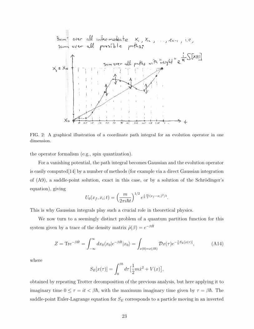
sian integrals over the momenta pn = p(tn). The a graphical visualization of the path-integral

is given in Fig.2.

The advantage of the path integral formulation is that it allows us to work with commut-

ing functions rather than noncommuting operators. It also very powerful for semi-classical

analysis with classical ~→ 0 limit emerges as its saddle point that extremizes the action. As

discussed in great detail in Feynman and Hibbs[14] and references therein, most problems

in quantum mechanics and field theory can be reproduced using this approach, often much

more efficiently. However, some problmes are much more amenable to treatment through

22

FIG. 2: A graphical illustration of a coordinate path integral for an evolution operator in one

dimension.

the operator formalism (e.g., spin quantization).

For a vanishing potential, the path integral becomes Gaussian and the evolution operator

is easily computed[14] by a number of methods (for example via a direct Gaussian integration

of (A9), a saddle-point solution, exact in this case, or by a solution of the Schrodinger’s

equation), giving

U0(xf , xi; t) =( m

2πi~t

)1/2

ei~m2

(xf−xi)2/t.

This is why Gaussian integrals play such a crucial role in theoretical physics.

We now turn to a seemingly distinct problem of a quantum partition function for this

system given by a trace of the density matrix ρ(β) = e−βH

Z = Tre−βH =

∫ ∞−∞

dx0〈x0|e−βH |x0〉 =

∫x(0)=x(β~)

Dx(τ)e−1~SE [x(τ)], (A14)

where

SE[x(τ)] =

∫ β~

0

dτ[12mx2 + V (x)

],

obtained by repeating Trotter decomposition of the previous analysis, but here applying it to

imaginary time 0 ≤ τ = it < β~, with the maximum imaginary time given by τ = β~. The

saddle-point Euler-Lagrange equation for SE corresponds to a particle moving in an inverted

23

potential −V (x). We note that this Euclidean action can also be obtained directly from the

real action (A13) by replacement it = τ with compact imaginary time β~. Immediately, we

can also obtain an analog of the Schrodinger’s equation in imaginary time, satisfied by the

density matrix

∂β ρ(β) = −Hρ(β).

We note that correlation functions computed with a path integral automatically give

time-ordered ones (operators are arranged in later ones appearing to the left),

Tr [T (x(τ1) . . . x(τn)ρ(β))] =

∫Dx(τ)x(τ1) . . . x(τn)e−

1~SE [x(τ)] (A15)

as it is only these time-ordered operators are arranged in the necessary order to apply the

Trotter decomposition to a correlation function.

Finally, generalizing this single variable coordinate path-integral to many variables, its

formulation for quantum field theory is straightforward. For example, a quantum partition

function for a phonon field u(r) in a continuum of an isotropic model is given by

Z =

∫u(r,0)=u(r,β~)

Du(r, τ)e−1~SE [u(r,τ)], (A16)

where

SE[u(r, τ)] =

∫ β~

0

dτddr

[1

2ρ(∂τu)2 +

1

2µ(∇u)2

].

We observe that in a path-integral formulation a d-dimensional quantum field theory

looks like a path integral of an effective “classical” theory in d+ 1 dimensions with the extra

imaginary time dimension confined to a slab 0 ≤ τ < β~.

At zero temperature β~ → ∞, leading to a classical like path-integral in all d + 1

dimensions. In contrast, at high temperature, β~ → 0, the field u becomes τ independent

(otherwise the time-derivatives cost too much action and are suppressed) and the partition

function reduces to that of a d-dimensional classical one

Z → Zcl =

∫Du(r)e−β

∫ddr 1

2µ(∇u)2

over time-independent classical phonon field u(r) with a Boltzmann weight controlled by

the elastic energy. This is indeed as expected, as quantum fluctuations are insignificant at

24

high temperature.

2. coherent states path-integral

From the derivation of the coordinate path-integral above, it is quite clear that other

equivalent representations are possible, determined by the basis set of the resolution of

identity in the Trotter decomposition. One particularly convenient representation is that of

coherent states |z〉

|z〉 = e−12|z|2eza

†|0〉 = e−12|z|2

∞∑n=0

zn√n!|n〉 (A17)

labelled by a complex number z. From the canonical commutation relation [a, a†] = 1 it

is clear that eza†

is an operator (analogously to ei~ cp for x) that shifts a’s eigenvalue of the

vacuum state |0〉 by z, leading to coherent state’s key property

a|z〉 = z|z〉.

These states are overcomplete with nontrivial overlap given by

〈z1|z2〉 = e−12|z1|2e−

12|z2|2ez1z2

and resolution of identity

1 =

∫d2z

2πi|z〉〈z| (A18)

where d2z2πi≡ dRezdImz

π.

Armed with these properties, we derive a very useful coherent-state path-integral. Using

the resolution of identity, (A18), we deduce Trotter decomposition of the density matrix,

〈zf |e−βH |zi〉 = 〈zN |e−ε~ H |zN−1〉〈zN−1|e−

ε~ H |zN−1〉 . . . 〈zj|e−

ε~ H |zj−1〉 . . . 〈z1|e−

ε~ H |z0〉.(A19)

25

where ε = β~/N . The matrix element can be evaluated for ε 1, given by

〈zj|e−ε~ H |zj−1〉 = 〈zj|zj−1〉

(1− ε

~〈zj|H|zj−1〉〈zj|zj−1〉

), (A20)

= 〈zj|zj−1〉e− ε~〈zj |H|zj−1〉〈zj |zj−1〉 = 〈zj|zj−1〉e−

ε~H(zj ,zj−1), (A21)

= e−12

[zj(zj−zj−1)−zj−1(zj−zj−1)]e−ε~H(zj ,zj−1). (A22)

where in the last line we simplified expression by taking the Hamiltonian H[a†, a] to be

normal-ordered (all a†s are to the left of a’s).

Putting this matrix element into the (A23), we find

〈zf |e−βH |zi〉 =

∫ N−1∏j=1

d2zj2πi

e−1~SE [zj ,zj] =

∫ z(0)=zi

z(β~)=zf

Dz(τ)Dz(τ)e−1~SE [z(τ),z(τ)], (A23)

in the second equality we took the continuum limit N → ∞, and the Euclidean action in

discrete and continuous forms is respectively given by

SE[zj, zj] =N−1∑j=1

[1

2zj(zj − zj−1)− 1

2zj(zj+1 − zj) +

ε

~H(zj, zj−1)

]+

1

2zf (zf − zN−1)− 1

2zi(z1 − zi), (A24)

SE[z(τ), z(τ)] =

∫ β~

0

dτ

[1

2(z∂τz − z∂τz) +

ε

~H[z(τ), z(τ)]

]+

1

2zf (zf − z(β~))− 1

2zi(z(0)− zi), (A25)

where the last terms involving zf , zi are boundary terms that can be important in some

situations but not in the cases that we will consider.

With this single-particle formulation in place, it is straightforward to generalize it to

many variables, and then by extension to a coherent-state path-integral formulation of a

quantum field theory. Applying this to bosonic matter, with identification a†, a→ ψ†, ψ and

z(τ), z(τ)→ ψ(τ, r), ψ(τ, r)

Z =

∫Dψ(τ, r)Dψ(τ, r)e−

1~SE [ψ(τ,r),ψ(τ,r)], (A26)

26

where the Euclidean bosonic action is given by

SE[ψ(τ, r), ψ(τ, r)] =

∫ β~

0

dτddr

[1

2~(ψ∂τψ − ψ∂τψ

)− ψ~

2∇2

2mψ

], (A27)

=

∫ β~

0

dτddrψ(~∂τ −~2∇2

2m)ψ, (A28)

with periodic boundary conditions on the bosonic field ψ(0, r) = ψ(β~, r) and its conjugate,

allowing us to integrate by parts to obtain the second form above. The action can also be im-

mediately obtained from the real-time action S, (??) by replacing it→ τ . A huge advantage

of this formulation is that it now allows us to calculation bosonic (time-ordered) correla-

tion functions using simple Gaussian integrals over commuting “classical” d+ 1-dimensional

fields, with the only price the extra imaginary time dimension, as compared to the classical

d-dimensional statistical field theory.

Fourier transforming the coherent bosonic fields,

ψ(τ, r) =1√β~∑ωn

∫ddk

(2π)dψ(ωn,k)eik·r−iωnτ , ψ(τ, r) =

1√β~∑ωn

∫ddk

(2π)dψ(ωn,k)e−ik·r+iωnτ ,

we obtain

SE[ψ(ωn,k), ψ(ωn,k)] =∑ωn

∫ddk

(2π)dψ(−i~ωn + εk)ψ, (A29)

where ωn = 2πβ~n is the bosonic Matsubara frequency.

[1] Pathria: Statistical Mechanics, Butterworth-Heinemann (1996).

[2] L. D. Landau and E. M. Lifshitz: Statistical Physics, Third Edition, Part 1: Volume 5 (Course

of Theoretical Physics, Volume 5).

[3] Mehran Kardar: Statistical Physics of Particles, Cambridge University Press (2007).

[4] Mehran Kardar: Statistical Physics of Fields, Cambridge University Press (2007).

[5] J. J. Binney, N. J. Dowrick, A. J. Fisher, and M. E. J. Newman : The Theory of Critical

Phenomena, Oxford (1995).

[6] John Cardy: Scaling and Renormalization in Statistical Physics, Cambridge Lecture Notes in

27

Physics.

[7] P. M. Chaikin and T. C. Lubensky: Principles of Condensed Matter Physics, Cambridge

(1995).

[8] “Chaos and Quantum Thermalization”, Mark Srednicki, Phys. Rev. E 50 (1994); arXiv:cond-

mat/9403051v2; “The approach to thermal equilibrium in quantized chaotic systems”, Journal

of Physics A 32, 1163 (1998).

[9] “Quantum statistical mechanics in a closed system”, J. M. Deutsch, Phys. Rev. A 43, 2046.

[10] J. Bartolome, et al., Phys. Rev. Lett. 109, 247203 (2012).

[11] D. M. Basko, I. L. Aleiner and B. L. Altshuler, Annals of Physics 321, 1126 (2006).

[12] “Many body localization and thermalization in quantum statistical mechanics”, R. Nandk-

ishore, D. Huse, Annual Review of Condensed Matter Physics 6, 15-38 (2015).

[13] D. Arovas, “Lecture Notes on Magnetism” and references therein. see “Magnetism” Boulder

School Lectures at http://boulder.research.yale.edu/Boulder-2003/index.html

[14] Quantum Mechanics and Path Integrals, R. P. Feynman and A. R. Hibbs.

[15] Statistical Mechanics Lectures’, R. P. Feynman.

28