Physiology based Mathematical Models for the Intensive ...

Physiology-based Mathematical Models for the Intensive

Care Unit: Application to Mechanical Ventilation

Antonio Albanese

Submitted in partial fulfillment of the

requirements for the degree of

Doctor of Philosophy

in the Graduate School of Arts and Sciences

COLUMBIA UNIVERSITY

2014

© 2014

Antonio Albanese

All rights reserved

ABSTRACT

Physiology-based Mathematical Models for the Intensive Care Unit:

Application to Mechanical Ventilation

Antonio Albanese

This work takes us a step closer to realizing personalized medicine, complementing

empirical and heuristic way in which clinicians typically work. This thesis presents

mechanistic models of physiology. These models, given continuous signals from a patient,

can be fine-tuned via parameter estimation methods so that the model’s outputs match the

patient’s. We thus obtain a virtual patient mimicking the patient at hand. Therapeutic

scenarios can then be applied and optimal diagnosis and therapy can thus be attained. As

such, personalized medicine can then be achieved without resorting to costly genetics.

In particular we have developed a novel comprehensive mathematical model of the

cardiopulmonary system that includes cardiovascular circulation, respiratory mechanics,

tissue and alveolar gas exchange, as well as short-term neural control. Validity of the model

was proven by the excellent agreement with real patient data, under normo-physiological as

well as hypercapnic and hypoxic conditions, taken from literature.

As a concrete example, a submodel of the lung mechanics was fine-tuned using real

patient data and personalized respiratory parameters (resistance, Rrs, and compliance, Crs)

were estimated continually. This allows us to compute the patient’s effort (Work of

Breathing), continuously and more importantly noninvasively.

Finally, the use of Bayesian estimation techniques, which allow incorporation of

population studies and prior information about model’s parameters, was proposed in the

contest of patient-specific physiological models. A Bayesian Maximum a Posteriori

Probability (MAP) estimator was implemented and applied to a case-study of respiratory

mechanics. Its superiority against the classical Least Squares method was proven in data-poor

conditions using both simulated and real animal data.

This thesis can serve as a platform for a plethora of applications for cardiopulmonary

personalized medicine.

i

Table of Contents

List of Figures ........................................................................................................................... i

List of Tables ............................................................................................................................x

Acknowledgments ................................................................................................................. xii

Dedication ...............................................................................................................................xv

Chapter 1: Introduction ..........................................................................................................1

1.1 Motivation ........................................................................................................................1

1.2 Thesis Organization .........................................................................................................7

1.3 Novel Contributions of the Thesis ...................................................................................8

Chapter 2: Cardiopulmonary Modeling ..............................................................................11

2.1 Introduction ....................................................................................................................11

2.2 History and Review of Cardiopulmonary Models .........................................................12

2.3 Model Development .......................................................................................................31

2.3.1 The Uncontrolled Cardiovascular System Model ................................................... 33

2.3.2 The Respiratory System Model .............................................................................. 42

2.3.3 The Gas Exchange and Transport Model................................................................ 45

2.3.4 The Cardiovascular Control Model ........................................................................ 53

2.3.5 The Respiratory Control Model .............................................................................. 57

2.4 Parameter Assignment ...................................................................................................63

2.4.1 Vascular System ..................................................................................................... 63

2.4.2 Heart ........................................................................................................................ 65

2.4.3 Lung Mechanics ...................................................................................................... 66

2.4.4 Gas Exchange and Transport .................................................................................. 67

2.4.5 Cardiovascular Control ........................................................................................... 69

2.4.6 Respiratory Control ................................................................................................. 70

2.5 Model Implementation ...................................................................................................71

2.6 Model Validation ...........................................................................................................74

2.6.1 Normal Resting Conditions .................................................................................... 74

2.6.2 Hypercapnia ............................................................................................................ 93

2.6.3 Isocapnic Hypoxia .................................................................................................. 97

2.6.4 Hypoxia ................................................................................................................... 99

Chapter 3: Work of Breathing and Respiratory Mechanics Estimation ........................101

3.1 Introduction ..................................................................................................................101

3.2 Respiratory Mechanics .................................................................................................102

3.2.1 State-of-art of Respiratory Mechanics Assessment .............................................. 104

ii

3.3 Work of Breathing (WOB) ..........................................................................................113

3.3.1 State-of-art of WOB Estimation ........................................................................... 113

3.4 Proposed Method .........................................................................................................117

3.4.1 Constraint Least-Squares (CLS) Algorithm ......................................................... 119

3.4.2 Modified Kalman Filter (MKF) Algorithm .......................................................... 124

3.5 Algorithm Validation ...................................................................................................131

3.5.1 Verification on Simulated Data ............................................................................ 131

3.5.2 Pig Test and Data Collection ................................................................................ 137

3.5.3 Validation on Real Data ........................................................................................ 138

3.6 Conclusion and Future Work .......................................................................................154

Chapter 4: Bayesian Parameter Estimation for Physiological Models ...........................156

4.1 Introduction ..................................................................................................................156

4.2 The General Parameter Estimation Problem ................................................................158

4.3 Bayesian vs Classical Parameter Estimation ...............................................................159

4.4 Maximum a Posteriori Probability (MAP) Estimator ..................................................161

4.5 MAP Estimator in the Gaussian Case ..........................................................................165

4.5.1 The Gaussian Case with Linear Model ................................................................. 166

4.6 Bayesian Estimation of Respiratory Mechanics ..........................................................167

4.6.1 Methods ................................................................................................................ 169

4.6.2 Results ................................................................................................................... 180

4.6.3 Discussion ............................................................................................................. 198

4.7 Conclusions and Future Work .....................................................................................199

Chapter 5: Summary and Future Research ......................................................................201

Bibliography .........................................................................................................................204

Appendix: Cardiopulmonary Model’s Equations ............................................................212

A1. The Circulatory System ..............................................................................................212

A.2 The Heart .....................................................................................................................214

A.3 The Lung Mechanics ...................................................................................................216

A.4 The Lung Gas Exchange .............................................................................................217

A.5 The Tissue Gas Exchange ...........................................................................................218

A.6 The Venous Pool Gas Transport .................................................................................219

A.7 The Respiratory Control ..............................................................................................220

A.8 The Cardiovascular Control ........................................................................................221

iii

List of Figures Figure 1.1 – Schematic of the current standard of diagnostic (Dx) and therapeutic (Tx)

medicine and source of information for CDSS. ................................................................. 2

Figure 2.1- Block diagram of the feedback control system described in Grodins et al. [10] .. 13

Figure 2.2 - Block diagram of the controlled system used in Grodins et al. [11]. V, flow rate;

F, air gas fraction; K, volume; Q, blood flow; C, blood gas concentration; MR,

metabolic rate; P, partial pressure. Subscripts: I , inspiratory ; E , expiratory; j, O2 or

CO2; A, alveoli; T, tissue; B, brain; CSF, cerebrospinal fluid; a, arteries; v, veins; ao,

aorta; aB, brain arteries; aT, tissue arteries; vT, tissue veins; vB, brain veins. ............... 14

Figure 2.3- Block diagram of the original Guyton’s 1972 model [15] .................................... 15

Figure 2.4 - Block diagram of the cardiovascular module in Guyton’s 1972 model [15]. QLO,

cardiac output from left heart; QRO, cardiac output from right heart; C, compliance ;

SA, systemic arteries; SV, systemic veins; RA, right atrium; PA, pulmonary artery; LA,

left heart; BFM, muscle blood flow; BFN, non-muscle blood flow; RBF, renal blood

flow. Figure adapted from [16]. ....................................................................................... 15

Figure 2.5 - Block diagram of HUMAN model showing the main physiological function

modules [18]. Modules’ names are as follows: HEART, calculation of blood flows and

cardiac output; CARDFUNC, strength of left and right heart; CIRC, general circulation;

REFLEX-1, sympathetic nerves ; REFLEX-2, parasympathetic nerves; TEMP,

thermoregulation; EXER, control of exercise; DRUGS, pharmacology; O2,oxygen

balance; CO2, carbon dioxide balance; VENT, control of ventilation; GAS, gas

exchange; HORMONES, basic renal hormones; KIDNEY, kidney function and status;

RENEX, kidney excretion; HEMOD, hemodialysis; FLUIDS, fluid infusion and loss;

WATER, water balance; NA, sodium balance; ACID/BASE, acid-base balance; UREA,

urea balance; K, potassium balance; PROTEIN, blood protein balance; VOLUMES,

blood distribution; BLOOD, blood volume and red cell volume. ................................... 18

Figure 2.6 - (Left Panel) The respiratory part of the model reported in [24]. Fs and Fp,

systemic and peripheral blood flow respectively; , alveolar ventilation; PiO2 and

PiCO2, oxygen and carbon dioxide concentration in the i-compartment respectively, i =

a,v,T, arteries, veins and tissues; MRO2 and MRCO2, oxygen and carbon dioxide

metabolic rate respectively. (Right panel) The cardiovascular part of the model as

reported in [24]. Ql and Qr, left and right cardiac output respectively; Pas and Pvs,

systemic arterial and venous pressure respectively; Pap and Pvp, pulmonary arterial and

venous pressure respectively; cl and cr, left and right ventricle compliance respectively;

Rl and Rr, left and right ventricle resitance respectively; Sl and Sr, left and right

ventricle contractility respectively; cas and cav, systemic artery and vein compliance

respectively; cps and cpv, pulmonary artery and vein compliance respectively; Rs and

Rv, systemic and pulmonary resistance respectively. ...................................................... 19

Figure 2.7 - (Left panel) Hydraulic analog of the cardiovascular system as reported in [5]. P,

pressures; R, hydraulic resistances; C, compliances; L, inertances; F, flows; sa, systemic

arteries; sp and sv, splanchnic peripheral and splanchnic venous circulation; ep and ev,

extrasplanchnic peripheral and extrasplanchnic venous circulation; mp and mv,

peripheral and venous circulation in the skeletal muscle vascular bed; bp and bv,

peripheral and venous circulation in the brain vascular bed; hp and hv, peripheral and

venous circulation in the heart (coronary vascular bed); la, left atrium; lv, left ventricle;

pa, pulmonary arteries; pp and pv, pulmonary peripheral and pulmonary venous

iiii

circulation; ra, right atrium; rv, right ventricle. (Right Panel) Block diagram describing

relationships among afferent information, efferent neural activities, and effector

responses as reported in [5]. Pb, baroreceptor pressure; PaO2, arterial PO2; Vt, tidal

volume; fab, fac, and fap, afferent activities from arterial baroreceptors, peripheral

chemoreceptors, and lung stretch receptors, respectively; θsh and θsp, offset terms for

the cardiac and peripheral sympathetic neurons describing the effect of the central

nervous system (CNS) hypoxic response; fsp and fsh, activity in efferent sympathetic

fibers directed to the vessels and heart, respectively; fv, activity in the vagal efferent

fibers; Rbp, Rhp, Rmp, Rsp, and Rep, peripheral resistance in the brain, heart, skeletal

muscle, splanchnic, and remaining extrasplanchnic systemic vascular beds; Vu,mv,

Vu,sv, and Vu,ev, unstressed volume in the skeletal muscle, splanchnic, and remaining

extrasplanchnic venous circulation; Emax,rv and Emax,lv, end-systolic elastance of the

right and left ventricle, respectively; T, heart period. ...................................................... 23

Figure 2.8 - (Left panel) Hydraulic analog of the cardiovascular system according to the

model in [30]. (Right Panel) Block diagram describing the baroreflex mechanism as

reported in [30]. See reference for explanation of symbols. ............................................ 25

Figure 2.9 - (Left panel) Physical model of the respiratory system as reported in [30]. (Right

Panel) Pneumatic analog of the model as reported in [30]. Patm, atmospheric pressure;

Ppl, intrapleural pressure; Pl,dyn, lung tissue dynamic elastic recoil pressure; Pc,

collapsible airways pressure; Pmus, respiratory muscle driving pressure; Ru, upper

airways resistance; Rc, collapsible airways resiatnce; Rs, small airways resistance; Rve,

lung tissue resistance; Cc, collapsible airways compliance; Cl, static lung tissue

compliance; Cve, dynamic lung tissue compliance; Ccw, chest wall compliance. ............ 26

Figure 2.10 - Block diagram of the cardio-respiratory model by Cheng et al. [39] . ............. 28

Figure 2.11 - Block diagram of the CP model. and , and gas

concentrations in the venous blood, respectively; and , and

arterial blood partial pressures, respectively; , arterial blood pressure; , pleural

pressure; , respiratory muscle pressure. ................................................................. 33

Figure 2.12 - Schematic diagram of the cardiovascular system. , pressure; , blood flow;

, mitral valve; , aortic valve; , tricuspid valve; , pulmonary valve.

Subscripts: , left atrium; , left ventricle; , left ventricle output; , systemic

arteries; , splanchnic peripheral compartment; , splanchnic veins; ,

extrasplanchnic peripheral compartment; , extrasplanchnic veins; , skeletal muscle

peripheral compartment; , skeletal muscle veins; , brain peripheral compartment;

, brain veins; , coronary peripheral compartment; , coronary veins; , thoracic

veins; , right atrium; , right ventricle; , right ventricle output; , pulmonary

artery; , pulmonary peripheral circulation; , pulmonary shunt; , pulmonary veins;

, pleural space. .............................................................................................................. 35

Figure 2.13 - Single-compartment windkessel-type model. , intravascular pressure; ,

outgoing blood flow rate; , resistance; , compliance; , inertance; , , ,

compartment index; , extravascular pressure reference (atmospheric pressure or

intrapleural pressure, depending on the value of ). ........................................................ 36

Figure 2.14 - Typical relationship of a blood vessel . , transmural pressure; ,

volume; , unstressed volume. Reproduced with permission from [46] ..................... 37

iiiii

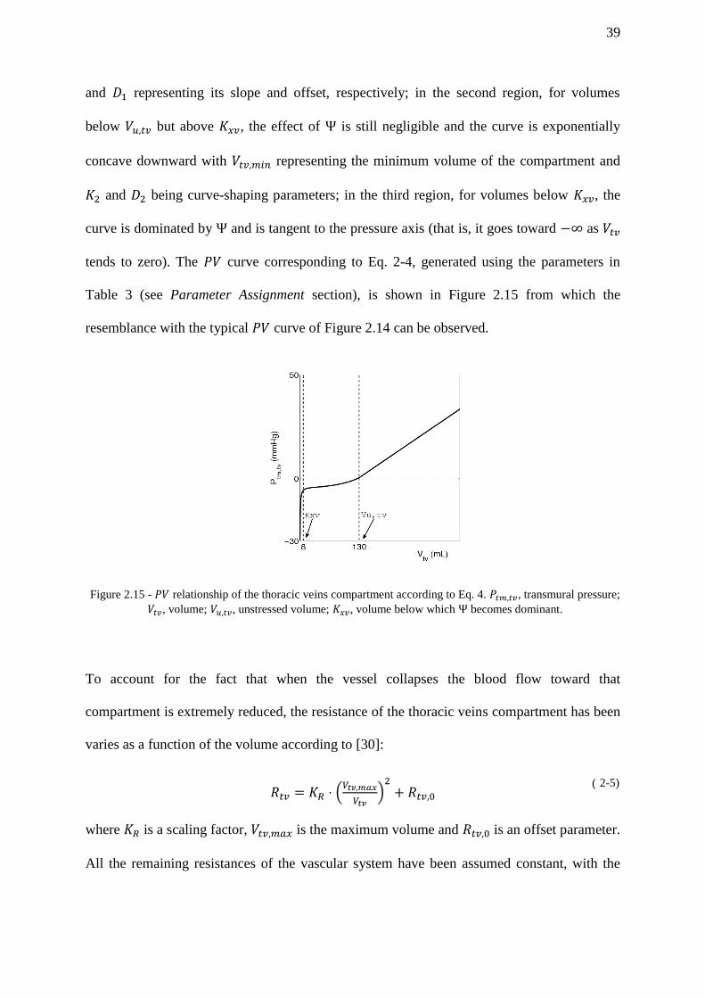
Figure 2.15 - relationship of the thoracic veins compartment according to Eq. 4. ,

transmural pressure; , volume; , unstressed volume; , volume below

which becomes dominant. ........................................................................................... 39

Figure 2.16 - Electrical analog of the left heart. and represent the mitral and the aortic

valve, respectively. , and are instantaneous pressure in the left atrium, left

ventricle and systemic arteries, respectively; is the left ventricle pressure in

isometric conditions; is the blood flow at the exit of the pulmonary veins, equals to

the blood flow entering the left atrium; and are blood flow entering the left

ventricle and blood flow leaving the left ventricle, respectively; and are

compliance of the left atrium and left ventricle, respectively; and are resistance

of the left atrium and left ventricle, respectively (note the transversal arrows in to

indicate the time-varying nature of this parameter); is the intrapleural pressure,

acting as reference external pressure on the heart. .......................................................... 41

Figure 2.17 - Lung mechanics model. , pressure; , resistance; , compliance; , total air

flow; , alveolar air flow. Subscripts: , airway opening; , larynx; , trachea; ,

bronchea; , alveoli; , pleural space; , chest wall ................................................... 43

Figure 2.18 - Schematic diagram of the gas exchange and transport model highlighting the

alveolar and tissue components, the venous pool gas transport block and the blood

transport delays. , arterial blood gas concentrations; , mixed venous

blood gas concentrations; , transport delay from lungs to systemic tissues; ,

transport delay from thoracic veins to lungs; , gas concentrations in the blood

that enters the tissue gas exchanger; , gas concentrations in the blood that enters

the lung gas exchanger; and , and gas flow between alveoli and

pulmonary capillaries, respectively; and , metabolic consumption and

production rates in the systemic tissues, respectively. The subscript indicates

either or . ............................................................................................................. 47

Figure 2.19 - Lung gas exchange model. , total air flow; , alveolar air flow; , dead

space volume; , alveolar volume; , gas fractions in the inspired air; ,

gas fractions in the dead space; , gas fractions in the alveoli; and ,

and gas flow between alveoli and pulmonary capillaries, respectively; , gas

concentrations in the blood that enters the pulmonary capillaries; , gas

concentrations in the pulmonary capillaries; , gas concentrations in the arterial

blood; , blood flow from the pulmonary arteries; , shunt percentage; , blood

flow at the exit of the pulmonary capillaries; , blood flow at the exit of the

pulmonary shunt compartment. ....................................................................................... 48

Figure 2.20 - Tissue gas exchange and venous pool gas transport model. , gas

concentration at the entrance of the systemic peripheral compartments; , gas

concentration in the combined blood-tissue compartment; , gas

concentrations in the systemic venous compartment; , gas concentrations

in the mixed venous blood; , blood flow at the exit of the systemic arteries; ,

blood flow at the exit of the systemic peripheral compartment; , blood flow at

the exit of the systemic venous compartment; , blood flow at the exit of the

thoracic veins; , blood volume contained in the systemic peripheral

compartment; , blood volume contained in the tissue compartment; ,

blood volume contained in the systemic venous compartment; , blood volume

contained in the thoracic veins; and , consumption and

production rates in the blood-tissue compartment, respectively. ......................... 51

ivii

Figure 2.21 - Cardiovascular control model. , venous concentration; ,

venous concentration; , arterial partial pressure; , arterial

partial pressure; , systemic arterial pressure; , tidal volume; , and ,

afferent firing frequency of barorecptors, peripheral chemoreceptors and lung stretch

receptors, respectively; , and , offset terms representing the effect of the

CNS ischemic response on the sympathetic fibers directed to peripheral circulation,

veins and heart, respectively; , and , activity in the efferent sympathetic

fibers directed to the peripheral circulation, the veins and the heart, respectively; ,

activity in the vagal efferent fibers; , , , and , systemic peripheral

resistance in coronary, brain, skeletal muscle, splanchnic and extrasplanchnic vascular

beds, respectively; , , , venous unstressed volume in skeletal

muscle, splanchnic and extrasplanchnic vascular bed, respectively; and

, end-systolic elastance of the left and right ventricle, respectively; HP, heart

period. .............................................................................................................................. 54

Figure 2.22 - Diagrams of time-dependent single-fiber responses of perfused carotid

chemoreceptors to up and down steps of CO2. Adapted from [62]. ................................ 57

Figure 2.23 - Schematic block diagram of the respiratory control model. , arterial

partial pressure; , arterial partial pressure; , respiratory muscle

pressure driving the lung mechanics model; and , basal values of

respiratory muscle pressure amplitude and respiratory rate, respectively;

and , variations in respiratory rate and respiratory muscle pressure amplitude

induced by the central chemoreceptors; and , variations in

respiratory rate and respiratory muscle pressure amplitude induced by the peripheral

chemoreceptors; , firing frequency of the afferent peripheral chemoreceptor fibers;

and , nominal value of and , respectively; and ,

time delay of the central and peripheral chemoreflex mechanisms, respectively;

and , gain factors for the central regulatory mechanism of amplitude and

frequency, respectively; and , gain factors for the peripheral regulatory

mechanism of amplitude and frequency, respectively; and , time

constant of the central regulatory mechanism of amplitude and frequency,

respectively; and , time constant of the peripheral regulatory mechanism of

amplitude and frequency, respectively. ................................................................ 59

Figure 2.24 – High level Simulink implementation of the CP Model. .................................... 73

Figure 2.25 – GUI of the CP Model; courtesy of Roberto Buizza, Philips Research North

America. ........................................................................................................................... 73

Figure 2.26- Left ventricle pressure and volume outputs. Left: time patterns of left ventricle

pressure (top) and volume (bottom). Dotted lines mark the four cardiac phases: a, filling

phase; b, isometric contraction phase; c, ejection phase; d, isometric relaxation phase.

Right: pressure-volume loop of the left ventricle. The four cardiac phases (a, b, c and d)

are shown along with the stroke volume SV and the opening and closing points of the

heart valves: 1, mitral valve closing point; 2, aortic valve opening point; 3, aortic valve

closing point; 4, mitral valve opening point. The two dotted lines tangent to the P-V loop

at the point 1 and 3 represent the diastolic and the end-systolic pressure/volume

functions, respectively. .................................................................................................... 77

Figure 2.27 - Pressure waveforms at different levels of the circulatory system.Top Left: time

patterns of left ventricle pressure, systemic arterial pressure and systemic splanchnic

peripheral vessels pressure. Bottom Left: time patterns of systemic pressure in the

vii

splanchnic venous compartment, thoracic veins pressure and right atrium pressure. Top

Right: time patterns of right ventricle pressure, pulmonary arterial pressure and

pulmonary peripheral vessels pressure. Bottom Right: time patterns of pulmonary veins

pressure and left atrium pressure. .................................................................................... 77

Figure 2.28 - Model-predicted flows (continuous line) compared with reported experimental

data (dashed line). Top: left ventricle output flow ( ). Bottom: right ventricle output

flow ( ). The experimental data have been redrawn from Fig. 7 of [30]. ............... 78

Figure 2.29 – Pressure, volume and flow waveforms generated by the lung mechanics model.

(A) From top to bottom: Respiratory muscle pressure ( ), pleural pressure ( ), alveolar pressure ( ), and air flow. (B) From top to bottom: Lung volume ( ),

alveolar volume ( ) and dead space volume ( ). ....................................................... 79

Figure 2.30 – Comparison between simulated and experimental airflow waveforms. Left

figure: pneumotachogram from a normal subject showing patterns of flow in nasal (both

quiet and rapid) and mouth breathing; reproduced from [87]. Right figure: model

generated airflow. Note that the scales of the two figures have been adjusted to allow

visual comparison. ........................................................................................................... 80

Figure 2.31 – Comparison between simulated and experimental pleural pressure waveforms.

(A) Tracing of pleural pressure from a dog in supine position during spontaneous

breathing; reproduced from [88]. (B) Model generated pleural pressure waveform. Note

that the time division in both figures is 1 sec and the scales of the two figures have been

adjusted to allow visual comparison. ............................................................................... 80

Figure 2.32 – Time profiles of model generated arterial and partial pressures. From

top to bottom: total lung volume ( ), partial pressure of oxygen in the arterial blood

( ) and partial pressure of carbon dioxide in the arterial blood ( )................ 85

Figure 2.33 – Time profiles of model generated mixed venous and partial pressures.

From top to bottom: total lung volume ( ), partial pressure of oxygen in the mixed

venous blood ( ) and partial pressure of carbon dioxide in the mixed venous blood

( ). .......................................................................................................................... 85

Figure 2.34 – Time profiles of and partial pressures in the dead space and alveolar

region. Top figure: CP Model outputs; Bottom figure: Lu et al. [30] model outputs. ..... 86

Figure 2.35 – Time profiles of and partial pressures in the alveolar space during a

respiratory cycle. Top figure: model simulations; Bottom figure: expected behaviour

from literature [90, 53]. .................................................................................................... 87

Figure 2.36 – Comparison between model generated partial pressures in the dead space

(Top figure) and a representative normal time-based capnogram (Bottom figure) [93]. . 88

Figure 2.37 - Mechanical effects of respiration on cardiovascular function. From top to

bottom: time profiles of intrapleural pressure ( ), venous return ( ), right ventricular

output flow ( ), right ventricular stroke volume ( ), left ventricular output flow

( ) and left ventricular stroke volume ( ). ........................................................... 91

Figure 2.38 - Mechanical effects of respiration on systemic arterial pressure. From top to

bottom: time profiles of intrapleural pressure ( ), systemic arterial pressure ( ),

systolic blood pressure ( ) and diastolic blood pressure ( ). ............................... 92

Figure 2.39 - Respiratory response to a 7% CO2 step input performed at 2 min and lasting 25

min. Continuous lines are model results; dashed lines are experimental data redrawn

viii

from [84]. Experimental data are means over 15 subjects. Figure courtesy of Limei

Cheng, Philips Research North America ......................................................................... 94

Figure 2.40- Respiratory response to 3, 5, 6 and 7% CO2 step input performed at 2 min and

lasting 25 min. Left: model simulations; Right: experimental data from [84].

Experimental data represent means over 10 subjects except for 7% which are means of

14 subjects. Figure courtesy of Limei Cheng, Philips Research North America ............ 95

Figure 2.41- Model predicted cardiovascular response to a 7% (red lines) and 8% (blue lines)

CO2 step input performed at 2 min and lasting 25 min. Figure courtesy of Limei Cheng,

Philips Research North America ...................................................................................... 96

Figure 2.42 - Respiratory response to a 8% O2 in air with controlled PACO2. The stimulus is

applied at 2 min and lasts 10 min. Continuous lines are model results; dashed lines are

experimental data redrawn from [83]. Experimental data are means over 10 subjects.

Figure courtesy of Limei Cheng, Philips Research North America ................................ 98

Figure 2.43 - Respiratory response to 8% inspired O2 in air with uncontrolled PACO2; step

input performed at 2 min and lasting 10 min. Left: model simulations;

Right:experimental data from [83]. Experimental data are means over 10 subjects.

Figure courtesy of Limei Cheng, Philips Research North America .............................. 100

Figure 3.1 – Schematic respresentation of the structures and pressures involved in breathing.

Pao, pressure at the airway opening; Pbs, body surface pressure (typically equal to

atmospheric pressure); Ppl, intrapleural pressure; Palv, alveolar pressure; PL,

transpulmonary lung pressure; Pw, chest-wall pressure; Prs, pleural difference across the

respiratory system. ......................................................................................................... 103

Figure 3.2–Schematic representation of mechanical ventilation showing the connection

between the patient and the ventilator. ET stands for endotracheal tube....................... 105

Figure 3.3 – Airway opening pressure profile during an Inspiratory Hold Maneuver. PEEP,

positive end-expiratory pressure; PIP, peak inspiratory pressure; Pplat, plateau pressure.

....................................................................................................................................... 106

Figure 3.4 – Examples of a correct EIP (left), when no patient’s respiratory muscles activity

is present, and an incorrect EIP (right), when patient’s respiratory muscles activity

generates artefacts in the airway pressure profile. Adapted from [97]. ......................... 107

Figure 3.5 – Simplified conceptual model of the respiratory system (left) and corresponding

electrical analog (right). Pao, airway opening pressure; Rrs, respiratory system resistance;

Crs, respiratory system compliance; Pmus, respiratory muscle pressure. ........................ 108

Figure 3.6 – Simplified conceptual model of the respiratory system (left) and corresponding

electrical analog (right) highlighting both the lung and the chest wall components. .... 111

Figure 3.7 – The esophageal balloon catheter. The pressure inside a latex balloon on the end

of a thin catheter is sensed by a pressure transducer connected to the proximal end. A

three-way stopcock permits injection of a small volume of air into the balloon so that its

sides clear the multiple holes in the end of the catheter. ............................................... 112

Figure 3.8 – Campbell diagram for a spontaneously breathing patient; reproduced from [107].

....................................................................................................................................... 114

Figure 3.9 – Input-output block diagram of the 1st oder single-compartment model of the

respiratory system. Pao, airway opening pressure; Pmus, respiratory muscle pressure; ,

air flow; V, lung volume; t, time. ................................................................................... 118

viiii

Figure 3.10 – Experimental profile of aiway pressure (Pao) and esophageal pressure (Pes)

obtained from a pig during an occlusion maneuver. The profile can be assumed as a

“gold standard” profile of Pmus. Figure courtesy of Francesco Vicario, Philips Research

North America ............................................................................................................... 121

Figure 3.11- Schematic diagram of the MKF algorithm. Figure courtesy of Dong Wang,

Philips Research North America. ................................................................................... 124

Figure 3.12- Schematic illustration of the MWLS algorithm. Figure courtesy of Dong Wang

and Francesco Vicario, Philips Research North America. ............................................. 126

Figure 3.13- Standrad formulation of the Kalman filter. Xk, true state varaible at time k; Xk-1,

true state variable at time k-1; uk, input to the system; zk, observed state at time k; Q,

covariance matrix of the process noise; R, covariance matrix of the observation noise;

Pk, error covariance matrix. ........................................................................................... 127

Figure 3.14 – Experimental profile of aiway pressure (Pao) and esophageal pressure (Pes)

obtained from a pig during an occlusion maneuver. The profile can be assumed as a

“gold standard” profile of Pmus. Note the different regions where different polynomial

orders can be used to locally approximate the actual Pmus profile. Figure courtesy of

Dong Wang, Philips Research North America. ............................................................. 128

Figure 3.15-Results of CLS estimation using the ASL5000 generated data. Figure courtesy of

Nikolaos Karamolegkos, Philips Research North America. .......................................... 133

Figure 3.16 - Zoomed version of Figure 3.15 highlighting the accuracy of the Pmus, Rrs and

Crs estimation obtained using the CLS apporach. Figure courtesy of Nikolaos

Karamolegkos, Philips Research North America. ......................................................... 134

Figure 3.17 - Results of MKF estimation using the ASL5000 generated data. Figure courtesy

of Nikolaos Karamolegkos, Philips Research North America. ..................................... 135

Figure 3.18 - Zoomed version of Figure 3.17 highlighting the accuracy of the Pmus, Rrs and Crs

estimation. Figure courtesy of Nikolaos Karamolegkos, Philips Research North

America. ......................................................................................................................... 136

Figure 3.19 – Validation results of the CLS algorithm under different PSV levels (20, 10 and

0 cmH2O). Pao, airway opening pressure; Rrs, respiratory system resistance; Crs,

respiratory system compliance; WOB, work of breathing. Data in green are noninvasive

estimates provided by the CLS algorithm; data in red are invasive gold standard

measurements obtained as described above (see 3.5.3 section). ................................... 142

Figure 3.20 – Validation results of the CLS algorithm under different PSV levels (20, 10 and

0 cmH2O). Pmus, respiratory muscle pressure. Data in green are noninvasive estimates

provided by the CLS algorithm; data in red are invasive gold standard measurements

obtained as described above (see 3.5.3 section). ........................................................... 143

Figure 3.21 – Validation results of the CLS algorithm under 5 PSV level and different FiCO2

levels (0, 2.5 and 5%). Pao, airway opening pressure; Rrs, respiratory system resistance;

Crs, respiratory system compliance; WOB, work of breathing. Data in green are

noninvasive estimates provided by the CLS algorithm; data in red are invasive gold

standard measurements obtained as described above (see 3.5.3 section). ..................... 144

Figure 3.22 – Validation results of the CLS algorithm under 5 PSV level and different FiCO2

levels (0, 2.5 and 5%). Pmus, respiratory muscle pressure. Data in green are noninvasive

estimates provided by the CLS algorithm; data in red are invasive gold standard


viiiii

Figure 3.23 – Regression analysis between estimated WOB by the CLS algorithm (y axis)

and gold standard WOB (x axis) under high PSV level (20-10 cmH2O) conditions. The

value of positive end expiratory pressure (PEEP) used in the corresponding experimental

condition is also reported in the legend. ........................................................................ 146

Figure 3.24 – Bland-Altman plot corresponding to the results in Figure 3.23. The WOB error

(y axis) is plotted against the gold standard WOB (x axis). Mean (dashed horizontal

lines) and ±1 std limits (solid horizontal lines) are also shown. ................................... 146

Figure 3.25 – Validation results of the MKF algorithm under different PSV levels (20, 10 and

0 cmH2O). Pao, airway opening pressure; Rrs, respiratory system resistance; Crs,

respiratory system compliance; WOB, work of breathing. Data in green are noninvasive

estimates provided by the MKF algorithm; data in red are invasive gold standard


Figure 3.26 – Validation results of the MKF algorithm under different PSV levels (20, 10 and

0 cmH2O). Pmus, respiratory muscle pressure. Data in green are noninvasive estimates

provided by the MKF algorithm; data in red are invasive gold standard measurements

obtained as described above (see 3.5.3 section). ........................................................... 150

Figure 3.27 – Validation results of the MKF algorithm under 5 PSV level and different

FiCO2 levels (0, 2.5 and 5%). Pao, airway opening pressure; Rrs, respiratory system

resistance; Crs, respiratory system compliance; WOB, work of breathing. Data in green

are noninvasive estimates provided by the MKF algorithm; data in red are invasive gold


Figure 3.28 – Validation results of the MKF algorithm under 5 PSV level and different

FiCO2 levels (0, 2.5 and 5%). Pmus, respiratory muscle pressure. Data in green are

noninvasive estimates provided by the MKF algorithm; data in red are invasive gold


Figure 3.29 – Regression analysis between estimated WOB by the MKF algorithm (y axis)

and gold standard WOB (x axis) under low PSV level (0-5 cmH2O) conditions. The

value of positive end expiratory pressure (PEEP) used in the corresponding experimental

condition is also reported in the legend. ........................................................................ 153

Figure 3.30 – Bland-Altman plot corresponding to the results in Figure 3.23. The WOB error

(y axis) is plotted against the gold standard WOB (x axis). Mean (dashed horizontal

lines) and ±1 std limits (solid horizontal lines) are also shown. ................................... 153

Figure 4.1 Classical vs Bayesian estimation .......................................................................... 161

Figure 4.2 Hit-or-miss cost function ...................................................................................... 163

Figure 4.3 – Experimental dataset from the animal test described in Chapter 3 corresponding

to a VCV breath with no spontaneous respiratory activity. From top to bottom: Pao is the

pressure measured at the airway opening; Flow is the air flow at the mouth; V is the

volume above FRC obtained by numerical integration of the flow signal; Pes is the

invasive esophageal pressure, surrogate for the intrapleural pressure. .......................... 170

Figure 4.4 – A priori probability density functions of the parameters for a general healthy

subject. From top to bottom: p.d.f. of Rrs; p.d.f. of Ers; p.d.f. of P0. .............................. 172

Figure 4.5 – A priori probability density functions of the parameters for an obstructive

disease subject. From top to bottom: p.d.f. of Rrs; p.d.f. of Ers; p.d.f. of P0. ................. 173

ixii

Figure 4.6 – A priori probability density functions of the parameters for a restrictive disease

subject. From top to bottom: p.d.f. of Rrs; p.d.f. of Ers; p.d.f. of P0. .............................. 174

Figure 4.7 – Results obtained via Bayesian estimation when using N=100 data points and

Gaussian prior distributions for different noise levels. A, low noise; B, medium noise; C,

high noise. Left plots are the p.d.f. of Rrs, middle plots are the p.d.f. of Ers and right plots

are the p.d.f. of P0. Blue curves indicate the a priori distributions, green curves indicate

the computed posterior distributions and red lines represent the true nominal parameter

values. ............................................................................................................................ 186






values. ............................................................................................................................ 187






values. ............................................................................................................................ 188

Figure 4.10 – Results obtained via Bayesian estimation at medium noise level when using

N=100 data points and prior distributions simulating an obstructive disease patient. Left

plots are the p.d.f. of Rrs, middle plots are the p.d.f. of Ers and right plots are the p.d.f. of

P0. Blue curves indicate the a-priori distributions, green curves indicate the computed

posterior distributions and red lines represent the true nominal parameter values. ....... 193

Figure 4.11– Results obtained via Bayesian estimation at medium noise level when using

N=100 data points and prior distributions simulating a restrictive disease patient. Left


P0. Blue curves indicate the a-priori distributions, green curves indicate the computed

posterior distributions and red lines represent the true nominal parameter values. ....... 193

Figure 4.12 – Experimental dataset from the animal test described in chapter 3 used to in the

2nd

stage validation step. From top to bottom: Pao, is the pressure measured at the airway

opening; Flow, is the air flow at the mouth; V, is the volume above FRC obtained by

numerical integration of the flow signal; Pes is the invasive esophageal pressure,

surrogate of the intrapleural pressure. ............................................................................ 195

Figure 4.13 – Results obtained via Bayesian estimation when using Gaussian prior

distributions for different number of data points N. A,N=100; B, N=50; C, N=10. Left


P0. Blue curves indicate the a priori distributions, green curves indicate the computed

posterior distributions and red lines represent the nominal parameter values. .............. 197

xii

List of Tables Table 2-1- Summary of existing cardiopulmonary models ..................................................... 30

Table 2-2 – Parameters of the vascular system in basal condition. See Eqs. A.1-A.29 in

Appenidx. Note the use of subscripts 0 and n in the unstressed volumes and resistances

that are subject to control mechanisms. Total blood volume (Vtot) is 5,300 mL. ............ 64

Table 2-3 – Parameters of the thoracic veins. See Eqs.2.4 -2.5 in the Model Development

section. See text and references for explanation of symbols. .......................................... 65

Table 2-4 – Parameters of the Heart model. See Eqs. A.30 – A.48 in the Appendix. .............. 65

Table 2-5 – Parameters of the lung mechanics model in basal conditions. See Eqs. A.49 –

A.60 in the Appendix. See text and Figure 2.17 for explanation of symbols and

subscripts. Note the use of subscripts 0 for the parameters that are subjects to control

mechanisms. ..................................................................................................................... 67

Table 2-6 – Parameters of the lung gas exchange model. See Eqs. A.61 – A.75 in the

Appendix. ......................................................................................................................... 69

Table 2-7 – Parameters of the tissue gas exchange model. See Eqs. A.76 – A.85 in the

Appendix. ......................................................................................................................... 69

Table 2-8 – Parameters of the cardiovascular control model modified with respect to [5, 6,

61]. ................................................................................................................................... 70

Table 2-9 – Parameters of the respiratory control model. See Eqs. 2.18 – 2.23 in the Model

Development section. is spikes/s................................................................................... 71

Table 2-10 – Number of state variables, parameters and outputs in the combined CP Model.

......................................................................................................................................... 72

Table 2-11- Static values of main hemodynamic variables ..................................................... 75

Table 2-12 – Mean values of the main gas composition variables. ......................................... 84

Table 2-13 – Steady-state changes in heart rate (HR), cardiac output (CO), total peripheral

resistance (TPR), mean arterial pressure (MAP), systolic blood pressure (SBP) and

diastolic blood pressure (DBP), in response to 7% and 8 % CO2 step input.

Experimental data are mean values from 8 subjects for the 7% case and from 10 subjets

for the 8% case . Data courtesy of Limei Cheng, Philips Research North America ....... 97

Table 4-1 - Results obtained via Bayesian MAP and LS estimation when using N=100 data

points and Gaussian prior distributions for different noise levels. The number in

parenthesis represent the coefficient of variation CV of the corresponding estimated

parameter. ...................................................................................................................... 189




parameter. ...................................................................................................................... 190




parameter. ...................................................................................................................... 191

xiii

Table 4-4 – Comparison between the numerical Bayesian MAP estimator and the analytical

MAP estimator. .............................................................................................................. 192

Table 4-5 - Results obtained via Bayesian MAP and LS estimation when using Gaussian prior

distributions for different number of data points N.The number in parenthesis represent

the coefficient of variation CV of the corresponding estimated parameter. .................. 196

xiiii

Acknowledgments

It is time for the acknowledgments and yet it is hard for me to realize that a very important

chapter of my professional career and life is about to end. If I picture myself a couple of years

ago, I would have never thought I could be able to write these pages. This PhD has been a

long and exciting journey and many people have contributed to this success. I can only hope

these words will make justice to those who have supported me throughout these years.

I’ll begin with my thesis supervisor and now colleague at Philips Research North

America, Dr. Nicolas W. Chbat. Nick is a fantastic advisor and without his help and

mentoring this work would have not been possible. I met Nick a while ago, while still

studying for my Master Degree, and ever since I have always found him an extremely useful

source of inspiration. His vision and passion for a quantitative approach to physiology and

medicine has driven my work and set my career goals throughout these years. Without him, I

would still be thinking that biomedical research is something confined to the walls of few

academic labs, detached from real world applications and industry. He has taught me that

physiology and medicine are fields that deserve to be studied and analyzed with the same

engineering rigour that is typically applied to traditional mechanical systems. With his work,

he has also taught me that if you truly believe in your research and you constantly fight for it,

then eventually people will recognize the importance of your work. This is an important

lesson that I will carry for my entire career and for this I am extremely grateful to him.

Throughout these years he has always been available for me, for academic, research and

personal advises, despite his very busy schedule even during nights and weekends. I believe

that such level of dedication and attention is reserved to very few lucky PhD students. Nick,

thanks for all you have done for me throughout these years!

xiiiii

My academic advisor at Columbia University, Professor Andrew Laine, has been very

helpful in guiding me throughout coursework and student’s life at Columbia, especially in the

first period of my studies when the US education system was a big challenge for me. He has

facilitated the development of this work in every possible way, providing me space and

resources in the Heffner Biomedical Imaging Lab at Columbia and making my time there as

pleasant as possible.

This work has been carried out in the Cardiopulmonary Group, led by Dr. Chbat at

Philips Research North America, and it would have not been accomplished without the help

and support of all the members of the team. All of them have contributed to my research and

for this I will always be grateful to them. Particularly, Dr. Dong Wang and Francesco

Vicario have tremendously contributed to the development of the estimation methods that are

described in Chapter 3 of this thesis. Dr. Limei Cheng has contributed to the

cardiopulmonary model development and validation, described in Chapter 2. Nikolaos

Karamolegkos has been tremendously valuable in any software/hardware interface related

issue, always ready to help, and he has been a very important player in the project. Roberto

Buizza has been the main contributor to the GUI development for the cardiopulmonary

model. I would also like to mention the contribution of Valentin Siderskiy, whose dedication

and work in the lab has laid down the basis for real-time applications of the modelling and

estimation methods described in this thesis. Finally, the interactions with Dr. Srini

Vairavan, Dr. Reza Sharifi, Dr. Syed Haider, Dr. Miriam Makhlouf and Caitlyn

Chiofolo have been very beneficial for my research and my professional development. On a

personal note, many people of the group have contributed in making my periods of research

at Philips as enjoyable as possible. A special thank goes to the “Mediterranean group”:

Roberto, Francesco, Nikos and Miriam, I feel lucky to have you as colleagues and friends,

and to be able to share with you work and life events.

xivii

I would also like to thank Dr. Adam Seiver, of Philips Healthcare Therapeutic Care

business unit, for very helpful discussions, ideas and support throughout this work.

Now comes the list of silent contributors. A big merit goes to my wife Anna for believing

in me, for pushing me to pursue my PhD studies, for being patient throughout these years and

for accepting the challenge of relocating to US and leave everything just to satisfy my

professional ambitions. Anna, you have proven to be the perfect life partner and without your

help I would have never been able to accomplish this. Thanks for your constant love and

support, especially in this last period of studies when you took all the family responsibilities

to allow me to focus on my thesis and complete my PhD journey in the best possible way.

Our little son, Pietro, who was born during this period of studies, has filled our lives and with

his smiles and laughs has helped me finding the energy needed to complete my PhD. Finally,

I would like to thank my parents, Enzo and Maria, for their unconditional love and support

during my entire life. You have thought me the most fundamental principles of life and how

these are important not only from a personal life perspective but also in your every-day

profession and work.

I thank Philips Research North America for providing a 4 year Van der Pol Fellowship

that has supported my studies and for providing an environment rich of intellectual and

material resources that have facilitated the development of this work. I feel privileged for

being able to perform my research in such environment.

xvii

Dedication

To my son and wife: without your love and care I could not have reached this point. I

dedicate this dissertation to you.

1

Chapter 1: Introduction

1.1 Motivation

Medicine is by and large an empirical field. Clinicians make diagnostic and therapeutic

decisions based on their experience. Evidence-based medicine is the current trend. It consists

in integrating individual clinical expertise with the best available external clinical evidence

from systematic research. Recently, strong effort has been put to help clinicians in their

decision making process via intelligent computerized systems (Clinical Decision Support

Systems, CDSS). The majority of these systems have focused on simply translating

clinicians’ current way of thinking into a set of rules (rule-based systems). Others have tried

to address the problem by exploiting the information contained in the data that are collected

from patients and looking for patterns or correlations (data mining/machine learning-based

systems). However, both approaches do not describe a complete picture to improve current

standard of care. A complementary alternative is to bring a mechanistic understanding of the

physiology via physiology-based mathematical models into the picture. Model-based

approaches can be used to:

1. Understand the cause-effect relationships of diseases and test new physiological

hypothesis.

2. Perform generic “what-if” scenarios and predict the effects of new therapies and

interventions on a generic patient (or class of patients).

3. Perform personalized ”what-if” scenarios on a specific patient to quantitatively

predict his/her response to different therapies or interventions. This leads to providing

optimal and personalized therapy (personalized medicine). To accomplish this, the

parameters of the physiological model will need to be fine-tuned to the specific

patient (patient-specific model) via parameter estimation techniques.

2

4. Probe the physiological system under exam and provide noninvasive estimates of

physiological variables and/or parameters that are otherwise hidden to the clinicians

due to the invasiveness, cost and patient discomfort that come with their

measurements. This information can be crucial for the assessment of patients’ health

status.

5. Detect and predict specific diseases.

Figure 1.1 shows a diagram of current standard of diagnostic and therapeutic medicine and

how different sources of knowledge can be used to build CDSS to improve current standard

of care. As highlighted in red, mechanistic physiology-based mathematical models can lead

to personalized medicine as opposed to population-based medicine. Two main advantages of

physiology-based models: they have the potential for optimizing diagnosis and therapy for

the individual patient, and they are more readily acceptable in the medical community. The

above comes with the understanding that a hybrid combination of two or all of the

approaches shown in Figure 1.1 may be needed for specific applications.

Figure 1.1 – Schematic of the current standard of diagnostic (Dx) and therapeutic (Tx) medicine and source of

information for CDSS.

3

This thesis is a small step toward reaching personalized medicine. We accomplish this

goal via advancing physiological modeling and parameter estimation. This work has been

carried out in the Cardiopulmonary Group led by Dr. Chbat at Philips Research North

America. The specific therapeutic application we choose is mechanical ventilation (MV).

MV is a commonly-used life-saving procedure. It is required when a patient is not able to

achieve adequate ventilation (and thereby gas exchange). This may occur under many

circumstances, for example in connection with surgery after anesthetics suppress the activity

of the respiratory muscles, or in acute respiratory failure caused by chronic obstructive

pulmonary disease (COPD), acute lung injury (ALI) or acute respiratory distress syndrome

(ARDS). It is estimated that MV is required by nearly 1.5 million patients in the United

States every year [1] and this number is set to increase. Most patients under MV would die

without one. Hence, MV is the most viable therapy available today for patients suffering of

respiratory failure.

However, since MV is not optimized for the specific patient, it can cause injury (8-10 %

of the cases, with a 2013 figure placing this range to 10-24%). A main issue with a ventilator

is that it exposes patients’ lungs to potentially destructive fluid/mechanical energy. As a

result, if MV is not optimized, ventilator-induced lung injury (VILI) can occur, exacerbating

existing conditions, prolonging length of stay in the ICU and increasing the risk of infection,

pneumonia and fatality due to multiple organ failure. Apart from patient safety and clinical

outcomes related concerns, there are also economic aspects associated with MV. The average

cost of a day in the ICU is somewhere between $3,518 [2] and $31,574 [3], depending on the

specific therapy used. Hence, an extra day under MV not only increases the risk of the patient

developing ventilator-related complications but also increases healthcare cost.

4

Although mechanical ventilation has been used in the ICU for many years, the

management of the mechanically ventilated patient is still largely based on empirical

knowledge. Particularly, selecting the best ventilation mode and adjusting the ventilator

settings as the conditions or the status of the patient change has remained a challenging task

even for the most experienced clinicians. This is due to the fact that the effects of ventilator

setting on the patient status are hardly predictable. The ventilator settings to be adjusted can

be many and each may have counteracting effects on the patient health. In fact, the degree of

interaction between the cardiovascular and the respiratory system is so high that often times

beneficial effects of ventilator resetting on one system are offset by detrimental effects on the

other system. For these reasons and given the limited time available for making clinical

decisions, ventilator settings adjustments are mostly driven by intuition or empirical

knowledge, rather than by quantitative mechanistic arguments. Furthermore, a trial-error

strategy is typically used when making ventilator settings adjustments. Clearly, this strategy

is suboptimal and may cause harm to the patient, as the effects of ventilator settings can only

be evaluated after these have been actually applied to the patient.

Standardized ventilator management protocols and guidelines do exist. However, these

are rigid generalized approaches, not tailored to the specific patient’s pathophysiology. As a

result, a high number of patients are still ventilated with sub-optimal ventilator settings. A

recent study [4] has shown that during 4 hours of conventional mechanical ventilation

according to clinical guidelines, only 12% of the times the patients were receiving

appropriate mechanical ventilation therapy.

In the ICU only arterial blood pressure (ABP), heart rate (HR), oxygen saturation (SpO2),

end-tidal CO2 (EtCO2) and very few other variables are monitored. Many other meaningful

clinical variables/parameters remain hidden, to the clinicians, as their monitoring would

require invasive procedures or interference with the normal operation of the ventilator. As a

5

result, since clinicians rely on available measurements to make diagnosis and therapeutic

decisions, their judgment and decisions are based only on a “partial” view of the patient

status. For instance, in spontaneous modes of MV (where patient can actively breathe),

quantitative assessment of patient respiratory efforts (Work of Breathing) is crucial in order

to avoid respiratory muscles atrophy or fatigue, and ultimately lead to liberation (or

weaning). However, this information (respiratory efforts assessment) can only be obtained

via invasive procedures, such as pleural pressure or esophageal pressure manometry, and

hence it is rarely offered at the bedside. Further, assessment of respiratory system’s

mechanics during MV is typically accomplished by measuring two parameters, termed

resistance (Rrs) and compliance (Crs). These two describe the resistive and elastic properties

of the respiratory system comprising airways, lung parenchyma and chest wall assuming a

simplistic model of the lung mechanics. Knowledge of these parameters allows to optimize

ventilation strategy or to even decide whether a therapeutic drug treatment is appropriate or

not for that particular patient. The most accepted technique to measure Rrs and Crs is the end-

inspiratory hold maneuver, which requires a fully relaxed patient. Even though this maneuver

is not invasive per se, it, however, interferes with the normal operation of the ventilator and

cannot be applied during spontaneous modalities of MV when the patient is actively

breathing. In these cases, monitoring of intrapleural pressure is required in order to offset the

effects of patient inspiratory activity, which comes with the drawback already mentioned

above. As a result, continuous monitoring of respiratory mechanics is not always done at the

bedside.

Physiology-based mathematical models (or physiological models) can help improve this

standard of MV therapy and can offer a valid tool to address some of the above limitations.

1. First, they can be used to quantitatively predict the patient response to ventilator

settings adjustments. Hence, by using patient-specific physiological models of the

6

cardiopulmonary system, the effects of a particular choice of ventilator settings could be

evaluated in virtual mode, without actually being applied to the patient.

2. Second, these models can be used to obtain continuous noninvasive estimates of those

physiological variables and/or parameters (WOB, Rrs, Crs, etc.) that are crucial to the

assessment of the health status but are not monitored at the bedside. The additional

information provided by these parameters and variables can be used, along with the already

available measurements from the patient, to form a ”complete” view of his/her health status.

This, in turn, provides better guidance for ventilator adjustments.

3. Third, since physiological models are a mathematical representation of the physical

system under exam, they can be used with advanced mathematical optimization or control

theory techniques, so to automatically select (closed-loop modality) ventilation strategy and

settings that would maximize/minimize an objective function or maintain certain

physiological variables within specific ranges. The closed-loop modality would also address

the current shortage of respiratory care practitioners at the bedside.

This thesis develops methods to promote the use of physiology-based mathematical

models of the cardiovascular and respiratory systems in order to improve current standard of

care in mechanical ventilation. In order to be useful in the clinical setting, a mathematical

model not only has to be accurate enough to capture the physiological mechanisms of the real

biological system (in our case the cardiopulmary system), but it also needs to become

“patient-specific” or “personalized”. Two fundamental ingredients are, hence, necessary in

order to accomplish our goal: 1) an accurate mathematical model of the cardiopulmonary

system; 2) efficient parameter estimation methods to fine tune the model to the particular

patient under study, thus making it “patient specific”. For this reason, the aim of this thesis

will be on both fronts of modeling and parameter estimation.

7

Our conjecture is that by taking full advantage of physiological models, mechanical

ventilation therapy will no longer be an ”art” dictated by assumptions based on empirical

knowledge, but rather a ”science” dictated by mechanistic understanding of the system under

exam and of the underlying physiological processes. The use of physiological model-based

clinical decision support (CDS) tools, or even closed-loop modalities, will eventually lead to

a drastic change in MV therapy: from shift-by-shift ventilator adjustments to breath-by-breath

personalized ventilation therapy - a major change in respiratory medicine.

1.2 Thesis Organization

The structure of this thesis is as follows:

Chapter 1 provides the introduction and motivation, and describes the scope, the

organization of the thesis and its novel contributions.

Chapter 2 provides a review of existing physiological models of the cardiopulmonary

system, emphasizing their limitation. It then describes the development and validation of a

novel comprehensive model that overcomes some of these limitations.

Chapter 3 provides a description of current techniques for respiratory mechanics and work

of breathing assessment, emphasizing their limitations. It then describes the development and

validation of a novel model-based approach for simultaneous estimation of respiratory

mechanics and work of breathing in spontaneously breathing mechanically ventilated

patients.

Chapter 4 provides a comparison between classic and Bayesian parameter estimation

techniques. It then describes the implementation of a Bayesian Maximum a Posteriori (MAP)

estimator and its application to a case-study of respiratory mechanics.

8

Chapter 5 concludes the dissertation and details future research directions arising from this

work.

1.3 Novel Contributions of the Thesis

The novel contributions of the thesis are:

1. Development and validation of a novel comprehensive model of the

cardiopulmonary system: several key improvements differentiate this model from

previous wok [5, 6]:

a. Inclusion of tidal breathing lung mechanics;

b. Inclusion of respiratory muscle pressure generator;

c. Inclusion of lung gas exchange model;

d. Inclusion of tissue gas exchange and venous blood transport models;

e. Development and inclusion of a novel respiratory control model;

f. Validation during hypercapnic, hypoxic and isocapnic hypoxic conditions.

This work has so far resulted in the following publications:

Albanese A, Cheng L, Ursino M, Chbat NW. A comprehensive mathematical

model of the human cardiopulmonary system: Model development, Am J Physiol

Heart Circ Physiol (submitted)

Cheng L, Albanese A, Chbat NW. A comprehensive mathematical model of the

human cardiopulmonary system: Sensitivity analysis and validation, Am J Physiol

Heart Circ Physiol (to be submitted April 2014)

Albanese A, Chbat NW, Ursino M. Transient respiratory response to hypercapnia:

analysis via a cardiopulmonary simulation model, in Proceedings of 33rd

Annual

International Conference of the IEEE EMBS, Boston, USA, 2011

Albanese A, Cheng L, Chbat NW. Cardiopulmonary simulator and medical devices

using cardiopulmonary simulator, Philips Invention Disclosure, January 2014

9

2. Development and validation of a novel technique for the assessment of

respiratory mechanics and patient’s efforts in spontaneously breathing

mechanically ventilated patients: several key features differentiate this technique

from existing methods [7, 8, 9] :

a. Suitable for both active and passive patients;

b. Noninvasive;

c. Model-based and hence physiologically interpretable;

d. Not interfering with normal ventilator operation;

e. Inclusion of physiologically based constrained;

f. The use of optimization techniques.

This work resulted in the following publications:

Albanese A, Karamolegkos N, Haider SW, Seiver A, Chbat NW. Real-time

noninvasive estimation of intrapleural pressure in mechanically ventilated patients: a

feasibility study. in Proceedings of 35th

Annual International Conference of the IEEE

EMBS, Osaka, Japan, 2013

Albanese A, Karamolegkos N, Haider SW, Seiver A, Chbat NW. Real-time Non-

invasive Pleural Pressure and Work of Breathing Estimation, Philips Technical

Report, February 2013

Chbat NW, Albanese A, Karamolegkos N, Haider SW, Seiver A. Real-time Non-

invasive Estimation of Work of Breathing, Patent Pending, February 2013

Albanese A, Vicario F, Wang D, Karamolegkos N, Chbat NW. Simultaneous

Estimation of Respiratory Mechanics and Patient’s Effort via Constrained

Optimization Method, Philips Invention Disclosure, January 2014

Wang D, Vicario F, Albanese A, Karamolegkos N, Chbat NW. Non-invasive

method for monitoring patient respiratory status via successive parameter estimation,

Philips Invention Disclosure, January 2014

10

3. Implementation of a Bayesian MAP estimator for respiratory mechanics: the

concept of MAP Bayesian estimation is known; however, to the best of our

knowledge it has never been applied to respiratory mechanics studies.

A conference and a journal papers are envisioned.

11

Chapter 2: Cardiopulmonary Modeling

2.1 Introduction

As mentioned in Chapter 1–Introduction, a prerequisite to the development of model-based

intelligent systems that optimize mechanical ventilation is the development of a

comprehensive and accurate mathematical model of the cardiovascular and respiratory

systems.

Mathematical representation of the mechanistic function of the cardiovascular and

respiratory systems is a challenging task. These two systems in humans interact via several

mechanisms, continuously, in a complex and non-linear manner. Oxygen (O2) and carbon

dioxide (CO2) are exchanged between pulmonary capillary blood and alveolar air, and the

efficacy of such exchange depends on the success of their coupling. Furthermore, the amount

of blood pumped by the heart and the degree of vessel vasoconstriction affect the blood gas

transport delay, which is a key determinant of O2 and CO2 blood contents. These, in turn,

modulate the depth and frequency of respiratory efforts via the action of specific receptors

(chemoreceptors), which become active when O2 and CO2 are out of their normal ranges. The

resulting increased tidal volume is sensed by receptors in the lungs that detects stretch of the

pulmonary tissues (lung stretch receptors). When activated, these receptors induce peripheral

vasoconstriction and bradycardia via modulation of the sympathetic and parasympathetic

(vagal) activities of the autonomic nervous system (ANS). Mechanical interactions also exist

due to the fact that the chest contains the respiratory system and a significant portion of the

cardiovascular system. These are particularly important during mechanical ventilation, when

elevated intra-thoracic pressure could compromise ventricular filling and stroke volume, thus

reducing arterial blood pressure (ABP). ABP, in turn, modulates the activity of specific

12

cardiovascular receptors (baroreceptors) that induce neural activity changes in both the

sympathetic and parasympathetic branches of the ANS, ultimately affecting heart rate,

cardiac contractility and vasomotor tone. Mechanisms outside ANS control also exist. Local

autoregulation and central nervous system (CNS) ischemic response are such examples.

These become active in extreme conditions, such as severe hypoxia, to preserve perfusion

and oxygen supply to vital organs (e.g brain and coronary arteries).

From the above description, it appears evident that the development of an accurate and

comprehensive mathematical model that accounts for such complex interactions is a

challenging task. Several physiological models of the cardiopulmonary system have been

proposed in the literature, but the majority are primarily either cardiovascular or pulmonary

and as such do not address their coupling. In this chapter, some of these existing

cardiopulmonary models are first reviewed, emphasizing their limitations and hence the need

for a novel integrative cardiopulmonary model. Then, the developed model will be described,

focusing on the new aspects with respect to previous models. Finally, model validation under

normal and pathological conditions will be shown via comparison with experimental data

from humans or animals.

2.2 History and Review of Cardiopulmonary Models

Pioneering work in cardiorespiratory modeling was started by Grodins and his colleagues in

the 1950s. To the best of our knowledge, Grodins was the first one to suggest the use of

control theory to describe the respiratory system and its regulation mechanisms. In the

seminal 1954 paper [10], Grodins and colleagues described the respiratory system as a

closed-loop feedback system (see Figure 2.1) where the controlled system (plant) was

represented by a combined lung-blood-tissue compartment, the controlled variable was the

13

tissue CO2 concentration, the controlling quantity was the pulmonary ventilation, the

disturbing quantity was the concentration of CO2 in the inspired air (FiCO2) and the

controlling system (controller + actuator) was represented by the combination of the

medullary respiratory centers (including the chemorecptors), the motor nerves to the

respiratory muscles and the ventilatory pump itself. The equations describing the lung-blood-

tissue compartment were derived based on first principles (conservation of mass), whereas

the equations describing the controlling system were derived based on empirical

observations. The resulting model was then described by a set of coupled non-linear

differential equations, whose solutions (obtained with the aid of an analog computer) yielded

predictions for the relationship between ventilation and arterial PCO2 that were in agreement

with the observed physiological responses.

Figure 2.1- Block diagram of the feedback control system described in Grodins et al. [10]

The model was subsequently expanded in 1967 [11] to include a more detailed description of

the plant and the effects of O2 and hydrogen ions (H+) on ventilation. The subsequent model

is shown in Figure 2.2. The controlled system was then represented by three compartments

(lung, brain and tissue) connected by the circulating blood. An additional cerebrospinal fluid

(CSF) compartment was also included in the model, as well as acid-base buffering, gas

transport delays and the effects of local autoregulation and chemoreceptors on cardiac output.

The model has formed the basis of much further work [12, 13, 14] and it is considered a

14

landmark achievement in the field. However, several limitations can be observed: 1) The

description of the plant is extremely simplified, with only three compartments representing

the whole system; 2) The events of the respiratory cycle are ignored and the lung is modelled

as a compartment of constant volume, uniform content, and no deadspace, ventilated by a

continuous unidirectional flow; 3) Description of the cardiovascular system is completely

neglected, hence the cardiac output is regarded as a nonpulsatile quantity, which can vary

only based on the O2 and CO2 blood contents via the action of chemoreceptors and local

autoregulation mechanisms.

Figure 2.2 - Block diagram of the controlled system used in Grodins et al. [11]. V, flow rate; F, air gas fraction;

K, volume; Q, blood flow; C, blood gas concentration; MR, metabolic rate; P, partial pressure. Subscripts: I ,

inspiratory ; E , expiratory; j, O2 or CO2; A, alveoli; T, tissue; B, brain; CSF, cerebrospinal fluid; a, arteries; v,

veins; ao, aorta; aB, brain arteries; aT, tissue arteries; vT, tissue veins; vB, brain veins.

Another seminal paper in the field was presented by Guyton and his co-workers in 1972

[15]. It describes the first large-scale integrated cardiovascular model that allowed for the

dynamic simulation of circulation, arterial pressure control mechanisms and body fluids

regulation. The description of the model in the original article was not given in terms of

mathematical equations, but in the form of a single graphical chart showing computing blocks

15

interconnected via wires (see Figure 2.3). The model is constructed around a central

circulatory dynamics module in interaction with 17 peripheral modules corresponding to

various physiological functions. The cardiovascular module distinguishes between left heart,

systemic arteries, systemic veins, right heart and pulmonary circulation (see Figure 2.4).

Figure 2.3- Block diagram of the original Guyton’s 1972 model [15]

Figure 2.4 - Block diagram of the cardiovascular module in Guyton’s 1972 model [15]. QLO, cardiac output

from left heart; QRO, cardiac output from right heart; C, compliance ; SA, systemic arteries; SV, systemic veins;

RA, right atrium; PA, pulmonary artery; LA, left heart; BFM, muscle blood flow; BFN, non-muscle blood flow;

RBF, renal blood flow. Figure adapted from [16].

16

The model includes autonomic regulation via the baroreceptors and chemoreceptors, local

autoregulation of blood flow, kidney dynamics, fluid shifts among circulation, interstitium

and cells, and the cardiovascular and renal effects of angiotensin, aldosterone and antidiuretic

hormone. As described by Thomas et al. [16], from a global standpoint the model is governed

by conservation relationships concerning sodium, potassium, oxygen, protein, water and

blood volumes in the circulatory loop. Each conservation relation is expressed by a set of

ordinary differential equations, which are combined with empirical curve fits of experimental

data. Despite the complexity and the high number of different physiological mechanisms

included, fundamental limitations of the model are: 1) Pulsatility of the heart is not

considered, hence all the variables computed by the model represent average values over the

heart cycle; 2) The model of autonomic regulation is not very accurate and because of the

absence of cardiovascular pulsatility, the model is inadequate to reproduce short-term

cardiovascular adjustments; 3) The description of gas exchange in the lungs, lung mechanics

and respiratory control is completely absent; 4) O2 dynamics are included in the model, but

due to the absence of a respiratory module their description does not obey to physiological

laws; for instance, O2 saturation is computed as a linear function of pulmonary fluid volume,

which seems a strong assumption; 5) The dynamics of CO2, which is known to play an

important role in cardiovascular regulation, are neglected; 6) Finally, the model mostly relies

on empirical relationships based on common physiological knowledge rather than first-

principles physiological laws. Nevertheless, Guyton’s model has been extensively considered

in the last decades and is currently used as a base for a number of research studies in the field

of physiology [16, 17].

Hence, we can conclude that Grodins and Guyton can be considered the “fathers” of

the field of cardiouplumonary modeling. However, due to the physiological knowledge and

limited computational power of the time, the interactions between the cardiovascular and

17

respiratory systems were not completely described in their early models. In the past few

decades, thanks to the advancement in computational technology, scientific activity in this

field has notably increased, and modeling complexity presented in the literature has grown to

more accurately describe physiological mechanisms and their dynamics. However, the

majority of these models, still remains primarily either cardiovascular or pulmonary and thus

do not permit a comprehensive exploration of cardiopulmonary response to different acute

conditions. Very few models have tried to address the strong dynamic interactions between

the cardiovascular and respiratory systems albeit with some limitations. In the following

sections, a brief review of some of these more recent models is provided.

Coleman et al. The model originally developed by Coleman, disciple of Guyton, in 1979

[18] and subsequently described by Coleman and Randall in 1983 under the name HUMAN

[19] is probably considered today the most comprehensive and largest model of physiological

functions. HUMAN is an extension of the 1972 Guyton’s model [15] and represents a truly

integrative simulator of the almost entire human physiology. It includes the circulatory

system, the respiratory system, the kidneys and body fluid volume control, the autonomic

nervous system, blood constituents, acid-base balance, thermo-regulation and some

hormones. A schematic block diagram representing most of these physiological modules is

shown in Figure 2.5. In HUMAN, some of the above mentioned limitations that characterized

his predecessor [15] have been overcome. Particularly, ventilation, gas exchange, and O2 and

CO2 dynamics based on conservation of mass principles have beeen included. However,

some other linitations have not been addressed: 1) The cardiovascular model is still

nonpulsatile, hence only average pressures and flows can be computed; 2) The respiratory

mechanics is not modeled and air flow into and out of the lungs is described using a simple

sinusoidal input function whose amplitude and frequency are controlled by a chemorceptor

model.

18

Figure 2.5 - Block diagram of HUMAN model showing the main physiological function modules [18]. Modules’

names are as follows: HEART, calculation of blood flows and cardiac output; CARDFUNC, strength of left and

right heart; CIRC, general circulation; REFLEX-1, sympathetic nerves ; REFLEX-2, parasympathetic nerves;

TEMP, thermoregulation; EXER, control of exercise; DRUGS, pharmacology; O2,oxygen balance; CO2,

carbon dioxide balance; VENT, control of ventilation; GAS, gas exchange; HORMONES, basic renal hormones;

KIDNEY, kidney function and status; RENEX, kidney excretion; HEMOD, hemodialysis; FLUIDS, fluid

infusion and loss; WATER, water balance; NA, sodium balance; ACID/BASE, acid-base balance; UREA, urea

balance; K, potassium balance; PROTEIN, blood protein balance; VOLUMES, blood distribution; BLOOD,

blood volume and red cell volume.

Nevertheless, HUMAN has been recognized and used worldwide as an important educational

tool and, over the years, has been constantly modified to reflect current physiological

knowledge and to keep up with technological advancement. In 2007, Abram et al. [20]

described the benefits of using an integrative model of human physiology for medical

education. The model was called Quantitative Circulatory Physiology (QCP) and represents

an extension of HUMAN. QCP, which is freely available online [21], was written and

compiled in C++ and this limited somehow the ability of the users to change or add

equations. For this reason a further version of the model, called HumMod, in which all the

model details are described in Extensible Markup Language (XML) files, was recently

developed by Hester and his collegues [22] and distributed as open source [23].

Batzel, Kappel and Tmischl: Cardiopulmonary dynamics and regulation has been the

object of several models proposed by researchers at the Institute for Mathematics and

19

Scientific Computing of the University of Graz. In 1998, a global model of the cardiovascular

and respiratory system was proposed by Timischl [24] as the result of her PhD research. The

model is divided into a respiratory component and a cardiovascular component, whose

schematic diagrams are shown in Figure 2.6. The respiratory component consists of lung and

lumped body tissue, connected by the circulating blood. The cardiovascular component

consists of the series arrangement of systemic and pulmonary circulation and includes the left

and right ventricles. Each circulation is lumped into 2 compartments, a single elastic artery

and a single elastic vein, connected by a single resistance vessel, accounting for both

arterioles and capillaries.

Figure 2.6 - (Left Panel) The respiratory part of the model reported in [24]. Fs and Fp, systemic and peripheral

blood flow respectively; , alveolar ventilation; PiO2 and PiCO2, oxygen and carbon dioxide concentration in

the i-compartment respectively, i = a,v,T, arteries, veins and tissues; MRO2 and MRCO2, oxygen and carbon

dioxide metabolic rate respectively. (Right panel) The cardiovascular part of the model as reported in [24]. Ql

and Qr, left and right cardiac output respectively; Pas and Pvs, systemic arterial and venous pressure

respectively; Pap and Pvp, pulmonary arterial and venous pressure respectively; cl and cr, left and right ventricle

compliance respectively; Rl and Rr, left and right ventricle resitance respectively; Sl and Sr, left and right

ventricle contractility respectively; cas and cav, systemic artery and vein compliance respectively; cps and cpv,

pulmonary artery and vein compliance respectively; Rs and Rv, systemic and pulmonary resistance respectively.

Gas exchange equations are imposed in the lungs and tissues based on conservation of mass,

in order to compute gas partial pressures in blood (PaO2, PaCO2, PvO2 and PvCO2). These

equations represent the linkage between the cardiovascular and respiratory systems and

assume O2 and CO2 tissue metabolic rates to be functions of workload intensity. The model is

20

used to simulate cardiorespiratory response to exercise. The non-linear system of differential

equations describing the model is solved at steady-state in resting conditions and for different

increasing workload levels. Different steady-state solutions correspond to different sets of the

parameters, which are dependent on the workload intensity. Transition from rest to exercise is

regulated by an optimal two-inputs/two-outputs controller that drives the system from the

steady-state characterizing the resting physiological condition to the steady-state

characterizing the exercise condition. Inputs to the controller are systemic arterial pressure,

Pas, and carbon dioxide arterial blood partial pressure, PaCO2. Outputs of the controller are

the changes in heart rate, H, and alveolar ventilation, . The transition between states is

optimal in the sense that the controller minimizes a cost functional in order to stabilize Pas

and PaCO2 such that deviations from their final steady-state values are as small as possible.

Hence, the optimal controller accounts for the cardiovascular control mechanism mediated by

the baroreceptors, and for the respiratory control mechanism mediated by the

chemoreceptors. The steady-state solution in terms of the main cardiorespiratory variables

showed a good level of agreement with both physiological and measured data. However,

despite the introduction of the original concept of optimal control, the model presents some

strong limitations: 1) The cardiovascular model is nonpulsatile, hence the model cannot

provide continuous intra-beat values for any of its output variables; 2) The lung is considered

as a single compartment ventilated by a continuous unidirectional stream of gas; the events of

the respiratory cycle are ignored and no description of the lung mechanics is included; 3) The

description of the cardiorespiratory control mechanisms is simplistic: the baroreceptors are

assumed to affect cardiovascular function only via changes in heart rate; systemic peripheral

resistance is assumed to be function of the exercise intensity and independent from baroreflex

stimulation; chemoreceptors are assumed to be acting upon the respiratory system via the

optimal controller based on PaCO2 values only; the effects of chemoreflex stimulation on the

21

cardiovascular system are completely neglected. The original model presented in [24] was

subsequently adapted in several studies. In 2000, Timischl et al. [25] extended the optimal

controller to account for PaO2 effects on ventilation and applied the model to simulate

transition from resting awake state to non-REM sleep. In 2005, Batzel et al. [26] further

revised the model in order to include the effects of transport delays between tissues and lungs

and vice versa. In 2004, Fink et al. [27] modified the cardiovascular component of the model

to distinguish between upper and lower compartments and simulate cardiorespiratory

response to orthostatic stress during head up tilt (HUT) experiments. Finally, in 2007, Kappel

et al. [28] further extended the model to simulate orthostatic stress induced by lower body

negative pressure (LBNP). However, despite few improvements in the description of the

control mechanisms, the limitations due to the absence of cardiovascular pulsatility and tidal

breathing lung mechanics still remained not addressed.

Ursino and Magosso: Several models of the cardiorespiratory system [5, 6, 13, 14] have

been developed by Ursino and Magosso, from the Department of Electronic Computer

Science and Systems of the University of Bologna. To the best of our knowledge, these

models provide the most complete quantitative description of the main physiological

mechanisms involved in short-term cardiopulmonary regulation. Particularly, the model in [5]

aims at describing the cardiovascular system and the adjustments involved in the response to

hypoxia. The model is an extension of a previous baroreflex model [29] developed by the

same authors, and it includes pulsatile left and right hearts, systemic and pulmonary

circulations, and some of the most important short term cardiovascular regulatory

mechanisms. The circulatory portion of the model (shown in Figure 2.7) is quite detailed,

including a total of 14 different compartments. An interesting feature of this model is that in

order to account for the differences in the sensitivity of the reflex mechanisms among specific

vascular districts, the peripheral and venous systemic circulations are divided into 5 different

22

compartments arranged in parallel: brain, skeletal muscle, coronary, splanchnic and

extrasplanchnic circulation. The cardiovascular control model (see Figure 2.7) is quite

detailed as well, including arterial baroreceptors, peripheral chemoreceptors and lung stretch

receptors, along with sympathetic and vagal neural pathways. The effects of the reflex

mechanisms on the cardiovascular function are mediated by changes in systemic peripheral

resistance, venous capacity, heart rate and left ventricular contractility. The effects of

peripheral chemoreceptors on ventilation are also included in the model, even though no

attempt to model the mechanics of the lung is made. In other terms, the tidal volume, which is

the input to the lung stretch receptors, is computed in the model as function of the peripheral

chemoreceptor activity without any description of the mechanical events that characterize the

respiratory cycle. Moreover, the model includes the local vasodilatory effect of O2

(autoregulation) on the brain, skeletal muscle and coronary circulation, and the

cardiovascular effects of CNS hypoxia (CNS ischemic response). The model was further

extended by the same authors in 2001 [6] to include the effects of CO2 on the cardiovascular

system and on minute ventilation. These additions allowed the model to simulate the response

to a variety of cardiovascular and respiratory challenges (hypoxia, hypercapnia, isocapnic

hypoxia, hemorrhage, etc.), and model predictions were shown to be in good agreement with

experimental data. However, due to the absence of the mechanical description of the lungs,

strong limitations can be found in these models: 1) Cardiorespiratory interactions via gas

exchange are not included; 2) PaO2 and PaCO2 cannot be directly computed and hence

remain external source inputs to the model, which therefore cannot be considered fully

closed-loop cardiopulmonary models.

If the focus of the above models [5, 6] was on cardiovascular regulation with only

minor details on respiratory control, the opposite is true for the models in [13, 14] developed

23

by the same authors. These are extensions of Grodins’ 1967 model [11], with additional

ventilatory control mechanisms, and as such suffer of the same limitations.

Figure 2.7 - (Left panel) Hydraulic analog of the cardiovascular system as reported in [5]. P, pressures; R,

hydraulic resistances; C, compliances; L, inertances; F, flows; sa, systemic arteries; sp and sv, splanchnic

peripheral and splanchnic venous circulation; ep and ev, extrasplanchnic peripheral and extrasplanchnic venous

circulation; mp and mv, peripheral and venous circulation in the skeletal muscle vascular bed; bp and bv,

peripheral and venous circulation in the brain vascular bed; hp and hv, peripheral and venous circulation in the

heart (coronary vascular bed); la, left atrium; lv, left ventricle; pa, pulmonary arteries; pp and pv, pulmonary

peripheral and pulmonary venous circulation; ra, right atrium; rv, right ventricle. (Right Panel) Block diagram

describing relationships among afferent information, efferent neural activities, and effector responses as reported

in [5]. Pb, baroreceptor pressure; PaO2, arterial PO2; Vt, tidal volume; fab, fac, and fap, afferent activities from

arterial baroreceptors, peripheral chemoreceptors, and lung stretch receptors, respectively; θsh and θsp, offset

terms for the cardiac and peripheral sympathetic neurons describing the effect of the central nervous system

(CNS) hypoxic response; fsp and fsh, activity in efferent sympathetic fibers directed to the vessels and heart,

respectively; fv, activity in the vagal efferent fibers; Rbp, Rhp, Rmp, Rsp, and Rep, peripheral resistance in the

brain, heart, skeletal muscle, splanchnic, and remaining extrasplanchnic systemic vascular beds; Vu,mv, Vu,sv,

and Vu,ev, unstressed volume in the skeletal muscle, splanchnic, and remaining extrasplanchnic venous

circulation; Emax,rv and Emax,lv, end-systolic elastance of the right and left ventricle, respectively; T, heart

period.

Lu et al.: Another very active group in the field of cardiopulmonary modeling is the

Dynamical System Group at Rice University, led by John W. Clark. This group has

developed several mathematical models [30, 31, 32] that, to our opinion, are the most

exhaustive in terms of gas exchange and cardiorespiratory mechanical interactions.

24

Particularly, the model proposed by Lu and his coworkers in 2001 [30] is an integrated

cardiopulmonary model aimed at simulating the Valsalva maneuver, an important clinical test

to assess baroreflex function. The model combines and extends previous models of blood

circulation [33], airway mechanics [34] and gas exchange [35] by the same group. The

cardiovascular portion of the model is quite detailed and consists of a lumped parameter

description of the four heart chambers, the systemic circulation and the pulmonary

circulation. The electrical analog of the cardiovascular model is shown in Figure 2.8. The

model of the heart is pulsatile and it includes the interacting ventricular free walls and

septum, the atria and the pericardium. The systemic circulation includes proximal and distal

aorta, proximal and distal arterioles, capillary and venous compartments, and vena cava.

Coronary and cerebral circulations are also described as purely resistance vessels, departing

from the aortic root and connecting to the vena cava. The pulmonary circulation is similarly

described and it also includes a purely resistive compartment mimicking the presence of the

pulmonary shunts. The cardiovascular control model (see Figure 2.8) includes arterial

baroreflex and sympathetic and vagal neural pathways. These affect cardiovascular function

via modifications of heart rate, myocardial contractility and vasomotor tone. The respiratory

component of the model is quite detailed as well and partition the airways into upper, middle

and small airways (see Figure 2.9). The upper airways are described as a rigid compartment

with a nonlinear flow dependent resistance. The middle airways are assumed collapsible and

are described by means of a nonlinear volume dependent resistance and a nonlinear P-V

relationship. The small airways, representing the alveoli and the lung tissue, are described as

a viscoelastic structure composed of a nonlinear compliance in series with the parallel

arrangement of a linear spring and a linear resistance. The alveolar region and the collapsible

airways are subjected to intrapleural pressure, which is the resultant of the pressure developed

by respiratory muscles and the chest wall elastic recoil. The gas exchange portion of the

25

model describes the changes in O2, CO2 and N2 concentrations within three compartments:

(1) the constant-volume dead space, represented by the rigid upper airways; (2) the variable-

volume mid airways; (3) the variable-volume alveolar compartment. For each species

considered, conservation of mass laws are imposed at both inspiration and expiration. In

writing the conservation law for the alveolar compartment, the diffusion of O2, CO2 and N2

across the alveolar-capillary membrane is considered.

Figure 2.8 - (Left panel) Hydraulic analog of the cardiovascular system according to the model in [30]. (Right

Panel) Block diagram describing the baroreflex mechanism as reported in [30]. See reference for explanation of

symbols.

26

Figure 2.9 - (Left panel) Physical model of the respiratory system as reported in [30]. (Right Panel) Pneumatic

analog of the model as reported in [30]. Patm, atmospheric pressure; Ppl, intrapleural pressure; Pl,dyn, lung tissue

dynamic elastic recoil pressure; Pc, collapsible airways pressure; Pmus, respiratory muscle driving pressure; Ru,

upper airways resistance; Rc, collapsible airways resiatnce; Rs, small airways resistance; Rve, lung tissue

resistance; Cc, collapsible airways compliance; Cl, static lung tissue compliance; Cve, dynamic lung tissue

compliance; Ccw, chest wall compliance.

The model produces results in agreement with physiological data for a normal resting subject

in supine position and during Forced Vital Capacity (FVC) and Valsalva maneuvers. In

comparison to previously described models, Lu’s model includes both a pulsatile cardiac

model and a tidal breathing lung mechanics with a good level of details in terms of

cardiopulmonary interactions. However, the model still presents some limitations: 1) The

description of the cardiovascular control mechanisms is simplistic, with only cardiovascular

baroreflex control included; 2) The respiratory control mechanisms are ignored; 3) Gas

exchange is described only at the alveolar-capillary membrane, neglecting gas exchanges in

tissues and other organs, and assuming that gaseous partial pressures in pulmonary arterial

blood (at the inlet of the alveolar-capillary membrane) are constant; 4) Due to the absence of

respiratory control mechanisms, the respiratory component of the model needs to be driven

by an external respiratory muscle pressure (or intrapleural pressure) source. In 2003, the

model was significantly extended by the same group of authors in order to overcome some of

27

these limitations [31]. The main new aspects of the model include the description of a lumped

peripheral tissue gas exchanger, which is linked to the lung gas exchanger via a circulatory

loop that incorporates transport delays. Moreover, peripheral chemoreceptors acting on both

the cardiovascular and respiratory systems have also been included, hence the driving

respiratory muscle pressure can be internally computed by the model. Finally, the model also

describes the lung stretch receptors and their effects on cardiovascular control. Despite these

substantial improvements, however, one fundamental point is still critical from our point of

view and makes this model unsuitable for studying acute conditions such as those related to

perturbations of CO2 arterial blood contents. The model, in fact, does not include description

of the central chemoreceptors, which under hypercapnic conditions play an important role in

respiratory system regulation. This limit was then eventually overcome in a further extension

of the model [52] by the same authors. Particularly, the central chemoreflex control of

respiration was added along with a detailed mathematical description of cerebral circulation,

cerebrospinal fluid dynamics, brain gas exchange and cerebral blood flow regulation. All

these modifications, however, were more cerebrovascular oriented, such that the model

became unnecessarily complex from a cardiopulmonary standpoint. Furthermore, in terms of

cardiovascular control mechanisms, the model did not reach the same level of details as

Ursino and Magosso’s model [6].

Cheng et al.: The department of Biomedical Engineering at the University of Southern

California, as part of a program dedicated to the advancement of biomedical system modeling

and simulation techniques (Biomedical Simulations Resource), has developed an integrated

cardiopulmonary model that takes the form of a software package, called PNEUMA, and that

is freely available online in its Matlab-SIMULINK implementation [36]. The model was first

introduced in 2002 [37] and it has been transformed over the years [38] until reaching its final

current stage described by Cheng et al. in [39]. The model is divided into a pulsatile

28

cardiovascular component, a tidal breathing respiratory component that includes lung gas

exchange, and a central neural control component, all interacting each other. A schematic

block diagram of the model highlighting the three different components is shown in Figure

2.10.

Figure 2.10 - Block diagram of the cardio-respiratory model by Cheng et al. [39] .

The model was applied to simulate transitions from sleep to awake state in normal and

disease conditions, hence a sleep mechanism module was also included (see Figure 2.10).

Both cardiovascular and central neural control components are largely based on Ursino and

Magosso’s model [6], with modifications that account for the effects of intrathoracic pressure

on the cardiovascular system and of sleep state on neural sympathetic and vagal activities.

The gas exchange and transport component is based on a model previously developed by

Khoo [40], which includes gas transport through the dead space, O2 and CO2 exchange in the

alveoli, and O2 and CO2 transport in blood. The dead space is modeled using 5 serially rigid

interconnected perfectly-mixed compartments where no gas exchange takes place. Mass

29

balance equations for O2 and CO2 are imposed during both inspiration and expiration

allowing for computation of breath by breath variations of O2 and CO2 partial pressures in

these 5 compartments. The alveoli are modeled as a single compartment whose volume

changes in synchrony with the breathing cycle. Mass balance equations for both species are

applied at the alveoli taking into account the amount of gas that is exchanged at the alveoli-

capillary membrane. Differential equations describing mass balance for O2 and CO2 are also

applied at the tissue level in order to relate gas concentrations in the venous blood to arterial

blood gas concentrations. The metabolic rate of the body tissues is assumed to be dependent

on the wakefulness state. The respiratory mechanics model distinguishes between upper

airways, lung tissues and chest wall dynamics. It is driven by a neuromuscular input that is a

function of chemoreceptors activation, sleep/awake state and a basal drive. The ventilation

control model computes the contributions from peripheral and central chemoreceptors to the

neuromuscular drive, and it is based on previous work by Khoo [40]. An interesting feature

of the model is that the sleep/awake state affects the upper airway conductance in a such a

way that during sleep the upper airway can collapse if a critical transmural pressure value is

reached. This allows the model to simulate obstructive sleep apnea (OSA). Furthermore, the

model is shown to be able to simulate several other interesting pathophysiological conditions

such as hypoxia, Cheyne-Stokes respiration and CPAP therapy effects on OSA patients.

Hence, we can conclude that the model presents several positive characteristics: high

versatility; pulsatile cardiovascular model and tidal breathing lung mechanics; detailed

cardiovascular control mechanisms deriving from Ursino and Magosso’s model [6].

However, despite these advantages, some limitations can be found: 1) Even though a

physiological model of respiratory mechanics is included, airflow in and out of the lungs is

computed using an empirical curvilinear equation [41] that relates lung volume to the

neuromuscular input; this choice seems to be arguable. 2) Gas exchange occurring outside of

30

the lungs (tissue metabolism) is modeled as taking place in a single tissue compartment and

correspondence with the 5 systemic compartments of the cardiovascular component [6] is

violated; 3) The inclusion of the interactions between sleep mechanisms and

cardiorespiratory system appears to be unnecessary for our purposes.

A summary of the above reviewed models in terms of their main features and limitations is

provided in Table 2-1 below. It is worth noticing that many other cardiouplmnary models

exist in the literature and have been applied to mechanical ventilation studies [42, 43, 44].

However, none of these models include cardiorespiratory control mechanisms and hence their

scope remain limited and they have not been considered in our review. Furthermore, other

models may exist but inevitably remain unknown to the author.

Table 2-1- Summary of existing cardiopulmonary models

31

As outcome of this review, the need for an integrative model of the cardiopulmonary system

that can overcome the limitations of these existing models becomes evident. This new model

should possess the following chracateristics: pulsatile cardiovascular and tidal breathing lung

mechanics components; detailed control mechanisms; detailed cardiorespiratory interactions.

This is the motivation behind the development of the model that is presented in the following

sections.

2.3 Model Development

The present cardiopulmonary model (CP Model) includes cardiovascular circulation,

respiratory mechanics and gas exchange, along with their main short-term control

mechanisms. The model incorporates essential features from existing models and represents a

substantial extension of the models by Ursino and Magosso [5, 6], which where chosen as our

starting point given their exaustive description of the neural control mechanisms (see Table

2-1). As described in the previous section, their models required arterial Po2 and Pco2 as

external input source, and completely ignored lung mechanics and gas exchange. Here,

separate sub-models of respiratory mechanics, gas exchange in lungs and tissues, gas

transport in blood, and respiratory control mechanisms have been added to attain a

comprehensive cardiopulmonary model that is able to run in closed-loop mode requiring

inspiratory air gas content (FiO2 and FiCO2) and total blood volume as the only inputs.

A schematic block diagram of the model is shown in Figure 2.11, where the

interconnections among the different subsystems are highlighted. The Cardiovascular System

and the Respiratory System interact via the Gas Exchange and Transport module. This

module describes the gas exchange processes that take place in the lungs and in the systemic

tissues, along with the gas transport throughout the circulatory system. Both the

32

cardiovascular and the respiratory systems are subject to their own specific control

mechanisms, identified in the block diagram as the Cardiovascular Control System and the

Respiratory Control System modules, respectively. Particularly, the cardiovascular function is

regulated by the Autonomic Nervous System (ANS) that integrates the afferent information

provided by the Baroreceptors, Peripheral Chemoreceptors and Lung Stretch Receptors.

Local Autoregulation mechanisms are also included along with a central nervous system

(CNS) mediated response to acute ischemic conditions (CNS Ischemic Response). The

respiratory function is assumed to be governed by the superposition of control mechanisms

mediated by both the Peripheral Chemoreceptors and the Central Chemoreceptors, which

modulates the activity of the Respiratory Muscles acting on the Lung Mechanics module.

This, in turn, can also be driven by the action of an external Mechanical Ventilator. In the

following sections, a qualitative description of these different components is provided.

Following a control-system theory approach, the cardiovascular and the respiratory system

are first described by the uncontrolled system (plant), in the absence of regulatory actions.

Description of their feedback control mechanisms is subsequently provided. A complete set

of equations describing the model is presented in the Appendix section.

33

Figure 2.11 - Block diagram of the CP model. and , and gas concentrations in the venous

blood, respectively; and , and arterial blood partial pressures, respectively; , arterial

blood pressure; , pleural pressure; , respiratory muscle pressure.

2.3.1 The Uncontrolled Cardiovascular System Model

The cardiovascular component of our CP Model is largely based on the work of Ursino and

Magosso [5, 6], however, some modifications have been introduced to allow a more detailed

description of the heart-lung interactions and integration with the lung mechanics and the gas

exchange modules. As shown in the schematic diagram in Figure 2.12, the model includes a

pulsating heart, a pulmonary circulation and a systemic circulation. The heart model includes

both left and right hearts along with their corresponding chambers (atrium and ventricles) and

valves (mitral, aortic, tricuspid and pulmonary valve). The systemic circulation is subdivided

into five distinct districts arranged in parallel and describing circulation into the coronary,

brain, skeletal muscle, splanchnic (comprising the liver, the spleen, and the gastro-intestinal

34

organs) and the remaining extrasplanchnic (kidney, skin, bones, etc.) vascular beds. This

distinction is necessary since, as it will be described later, autonomic and local cardiovascular

regulatory mechanisms exert different actions on each compartment. The hemodynamic in

both systemic and pulmonary circulations distinguish between large arteries, peripheral

vessels (which combine arterioles and capillaries) and veins. The modifications with respect

to the original model formulation presented in [5, 6] are the following: 1) A pulmonary shunt

compartment has been added in parallel to the pulmonary peripheral circulation, between the

pulmonary artery and the pulmonary veins (anatomical shunting) to account for the normal

physiological amount of blood that does not pass through the pulmonary capillaries and does

not participate in gas exchange. We are aware that this is a high simplification as the

anatomical shunts are mostly due to the bronchial circulation and the thebesian veins, which

are both not located between the pulmonary arteries and the pulmonary veins. However, our

representation is not intended to have anatomical correspondence and is only used to include

a circulatory branch that bypasses pulmonary gas exchange. 2) An additional compartment,

representing the thoracic veins, which return blood to the right atrium, has been included in

the systemic circulation. 3) The effects of respiration on venous return and cardiac output

(respiratory pump) have been modeled by considering intrapleural pressure ( ) as the

reference extravascular pressure for those compartments that are located inside the thoracic

cavity (heart, lungs and thoracic veins); all remaining compartments are assumed to be

subject to extravascular atmospheric pressure ( ). 4) As a consequence of respiration,

transmural pressure in the systemic veins can become negative at their point of entrance in

the thoracic cavity; to account for this phenomenon, venous valves have been included by

inserting an ideal diode both upstream and downstream of each systemic venous

compartment, thus preventing retrograde blood flow [45]. With these modifications, the

model includes a total of 20 compartments that are listed in details in Figure 2.12.

35

Figure 2.12 - Schematic diagram of the cardiovascular system. , pressure; , blood flow; , mitral valve; ,

aortic valve; , tricuspid valve; , pulmonary valve. Subscripts: , left atrium; , left ventricle; , left

ventricle output; , systemic arteries; , splanchnic peripheral compartment; , splanchnic veins; ,

extrasplanchnic peripheral compartment; , extrasplanchnic veins; , skeletal muscle peripheral compartment;

, skeletal muscle veins; , brain peripheral compartment; , brain veins; , coronary peripheral

compartment; , coronary veins; , thoracic veins; , right atrium; , right ventricle; , right ventricle

output; , pulmonary artery; , pulmonary peripheral circulation; , pulmonary shunt; , pulmonary veins;

, pleural space.

1) The Circulation Model: Each vascular compartment shown in Figure 2.12 is described

trough traditional windkessel models, i.e. as the arrangement of a hydraulic resistance ( ),

which accounts for pressure energy losses, and a hydraulic compliance ( ), which

determines the blood volume stored in each compartment at a given pressure. For those

compartments where inertial forces in blood are relevant, i.e. large pulmonary and systemic

arteries, inertance ( ) is also included as a third parameter of the corresponding windkessel-

36

type model. The general 3-element windkessel single-compartment model structure is

illustrated in Figure 2.13.

Figure 2.13 - Single-compartment windkessel-type model. , intravascular pressure; , outgoing blood flow rate;

, resistance; , compliance; , inertance; , , , compartment index; , extravascular pressure

reference (atmospheric pressure or intrapleural pressure, depending on the value of ).

Equations relating pressures ( ) and flows ( ) in the vascular system are obtained by

enforcing conservation of mass principles for each vascular compartment of Figure 2.12.

Hence, in the general case of a 3-element vascular compartment such as the one of Figure

2.13, the following two ordinary differential equations (ODEs) hold:

2-1)f

2-2)f

where , and represents volume, outgoing flow and pressure of the -th compartment,

respectively (see Figure 2.13 legend for further definitions of subscripts). The two equations

above need to be combined with the corresponding pressure-volume ( ) relationship of the

-th compartment, in order to solve for the pressures . The typical relationship of a

blood vessel (artery or vein) is shown in Figure 2.14 below.

(

(

37

Figure 2.14 - Typical relationship of a blood vessel . , transmural pressure; , volume; , unstressed

volume. Reproduced with permission from [46]

It is quite linear near the unstressed volume (volume at zero transmural pressure), concaves

upward, gradually increases in slope at higher volumes, and concaves downward as the

volume decreases and the vessel collapses. Arteries and capillaries are typically subject to

high transmural pressure values and the operating point along the curve is such that a

linear approximation is valid [47, 48]. Hence, in the model, the relationships of the

systemic arterial and peripheral compartments have been assumed linear over the entire

pressure range examined. This is also the common choice in the majority of the lumped-

parameter models of the circulatory system that have been presented in the literature [49, 50].

Analogously, the entire pulmonary circulation (including arteries, peripheral and venous

compartments) is also assumed to be characterized by linear relationships. The

assumption of linear relationship allows for constant and pressure independent

compliances . Hence the volume of each of these compartments is computed as the sum of

the unstressed volume component ( ) and the excess volume component ( ), which is

associated with the increase in the transmural pressure:

38

(

⏟

2-3)f

where is the transmural pressure of the -th compartment. On the contrary, the

hypothesis of linear relationship does not always hold for the venous circulation.

Particularly, while in most of the venous circulation the pressure inside the vessels is greater

than the external pressure and the operating point on the curve is such that the linear

approximation still holds, in the vena cava, and in the thoracic veins in general, the

transmural pressure is typically small and can become negative under the influence of a

positive intrathoracic pressure. In these cases, the nonlinear nature of the relationship

becomes important [46] (see Figure 2.14). For this reason, the same linear relationship

above (Eq. 2-3) has been used for the systemic venous compartments (splanchnic,

extrasplanchnic, skeletal muscle, brain and coronaries), whereas the thoracic veins have been

modelled via a non-linear collapsible relationship. This has been derived by combining

features of slightly different curves proposed in the literature for the vena cava

compartment [39, 30, 51]:

{ ( )

2-4)

where and are the transmural pressure and the volume of the thoracic veins

compartment, respectively. Note that is a curvilinear function that is negligible at volumes

above and dominates the relationship in the region of collapse, when the volume of

the vessel is very small [51]. Hence, according to Eq. 2-4, the curve of the thoracic veins

compartment is characterized by 3 different regions: in the first region, for volumes above the

unstressed value , the effect of is negligible and the curve is essentially linear with

(

39

(

and representing its slope and offset, respectively; in the second region, for volumes

below but above , the effect of is still negligible and the curve is exponentially

concave downward with representing the minimum volume of the compartment and

and being curve-shaping parameters; in the third region, for volumes below , the

curve is dominated by and is tangent to the pressure axis (that is, it goes toward as

tends to zero). The curve corresponding to Eq. 2-4, generated using the parameters in

Table 3 (see Parameter Assignment section), is shown in Figure 2.15 from which the

resemblance with the typical curve of Figure 2.14 can be observed.

Figure 2.15 - relationship of the thoracic veins compartment according to Eq. 4. , transmural pressure;

, volume; , unstressed volume; , volume below which becomes dominant.

To account for the fact that when the vessel collapses the blood flow toward that

compartment is extremely reduced, the resistance of the thoracic veins compartment has been

varies as a function of the volume according to [30]:

(

)

2-5)

where is a scaling factor, is the maximum volume and is an offset parameter.

All the remaining resistances of the vascular system have been assumed constant, with the

40

exception of those of the systemic peripheral compartments that are assumed to vary under

the action of feedback regulatory mechanisms (see Cardiovascular Control Model section).

The effects of gravity on the cardiovascular system have been neglected. Hence, the

model is suitable for simulating subjects in the supine position only, when no hydrostatic

pressure gradient across different compartments is present. Furthermore, since the five

systemic peripheral vessels are assumed in parallel and no gravitational effects are

considered, the pressures inside each compartment are assumed to be equal. Analogous

reasoning applies to the pulmonary shunt and the pulmonary peripheral compartments (see

Figure 2.12). Finally, note that in solving the model equations for the pressure variables,

atmospheric pressure has been assumed to be zero and hence the resulting values of

represent above-atmospheric and not absolute pressure values.

2) The Heart Model: The model of the pulsating heart remains unchanged compared

to that one used in [5, 6], where an accurate description can be found. The only modification

that has been introduced is the inclusion of the intrapleural pressure as the external reference

pressure acting outside the heart chambers. Briefly, the models of the left and right heart are

essentially equivalent with different parameter values. The electrical analog of the heart

shown in Figure 2.16 pertains to the left heart. Each atrium is described as a passive chamber,

characterized by a linear PV relationship with constant values of compliance and unstressed

volume. Hence, the contractility of the atrium is neglected. Blood passes from the atria to the

ventricles through the atrioventricular valves (mitral valve, MV, and tricuspid valve, TV),

modelled as ideal unidirectional diodes and connected in series with the corresponding

constant atrium resistances. The equations relating pressures and flows in the atria are

obtained by combining mass balance equations, similar to Eq. 2.3, with the corresponding

linear PV relationship. The activity of the ventricles is modelled by means of a variable-

elastance model, which accounts for the isometric pressure-volume function, and a time-

41

varying resistance, which reflects the viscous forces in the ventricle. The elastance varies

during the cardiac cycle as a consequence of the contractile activity of the ventricle. At

diastole, the ventricle fills through an exponential pressure-volume function, while at end

systole the pressure-volume function is linear and its slope (called the end-systolic elastance)

is denoted by . Shifting from the end-diastolic to the end-systolic relationship is

governed by a pulsating activation function with period HP equals to the heart period.

The duration of systole is assumed to decrease linearly with the heart period, which in turn is

modulated by the control action of the ANS (see Cardiovascular Control Model section).

Finally, blood flow leaving the ventricles depends on the opening of the aortic or pulmonary

valve and on the difference between the isometric ventricle pressure and the downstream

pressure (systemic arterial pressure or pulmonary artery pressure, depending on whether right

or left ventricle is considered). Detailed equations describing the heart model can be found in

[5] and are also reported in the Appendix section.

Figure 2.16 - Electrical analog of the left heart. and represent the mitral and the aortic valve,

respectively. , and are instantaneous pressure in the left atrium, left ventricle and systemic arteries,

respectively; is the left ventricle pressure in isometric conditions; is the blood flow at the exit of the

pulmonary veins, equals to the blood flow entering the left atrium; and are blood flow entering the left

ventricle and blood flow leaving the left ventricle, respectively; and are compliance of the left atrium and

left ventricle, respectively; and are resistance of the left atrium and left ventricle, respectively (note the

transversal arrows in to indicate the time-varying nature of this parameter); is the intrapleural pressure,

acting as reference external pressure on the heart.

42

2.3.2 The Respiratory System Model

As shown in Figure 2.11, the model of the respiratory system includes description of the lung

mechanics and of the respiratory muscles. The lung mechanics portion is based on previous

work by Rideout and Fukui [52, 53] and has been modified to include chest wall and

intrapleural pressure dynamics. shows the equivalent pneumatic circuit representing the lung

mechanics model. It consists of the series arrangements of four segments, namely the larynx,

the trachea, the bronchea and the alveoli. Each segment has been represented by a linear

resistance and a linear compliance, which describe the dissipative and the elastic forces that

act on the respiratory system during normal breathing. Inertial forces have not been

considered because they have negligible effects within the physiological breathing

frequencies [54]. The model can be driven by either an external pressure representing

the pressure provided by the ventilator, as in the case of mechanically ventilated patients, or

by an internal generator representing the pressure generated by the respiratory muscles,

as in the case of spontaneously breathing patients. Note that is a fictitious variable that

does not correspond to a physical quantity. In a spontaneously breathing subject, in fact,

represents the equivalent pressure that has to be applied outside the thorax if the respiratory

muscles were paralyzed in order to maintain normal respiratory flow, volume and pressure

waveforms [55]. The chest wall has been modeled as a passive compliant element whose

pressure-volume characteristic has been assumed linear and hence described by a constant

compliance term, . This is a good approximation in the volume range of quite breathing

(2.5 to 3 L), according to the typical assumption of sigmoidal relationship [34]. Chest

wall viscous resistance to flow has been neglected, as this has typically a small contribution

to the overall respiratory system resistance in both health and disease states [56, 57]. The

respiratory muscle generator is connected to the chest wall compliance, which acts on the

43

pleural space whose internal pressure is transferred to those segments lying within the

chest cavity, i.e. trachea, bronchea and alveoli.

Figure 2.17 - Lung mechanics model. , pressure; , resistance; , compliance; , total air flow; , alveolar air

flow. Subscripts: , airway opening; , larynx; , trachea; , bronchea; , alveoli; , pleural space; , chest

wall

In the present study, since the model was used to simulate spontaneous breathing

conditions, the action of the external pressure generator is nullified and the airway

pressure is always assumed to be equal to atmospheric pressure. However, the external

pressure generator could be restored in order to simulate artificial ventilation conditions, or

even superimposed to the action of the internal pressure generator to account for

simultaneously natural and artificial breathing.

The respiratory muscle pressure (internal pressure generator), , has been modelled

based on the average profile proposed by Mecklemberg [58], obtained from experimental

flow and pressure data collected from a group of 12 adult healthy subjects breathing

spontaneously from atmosphere. The experimental muscle pressure curve has been

44

reproduced as a piece-wise continuous function consisting of an inspiratory parabolic profile

and an exponential expiratory profile. Particularly, under the assumption of complete passive

exhalation with no recruitment of the expiratory muscles (reasonable for minute ventilation

values up to 40 L/min [59]), is assumed to decrease from 0 to its minimum end-

inspiratory value during the inhalation phase and to gradually return to 0 during exhalation,

according to:

{

( 2-6)

where and represent the duration of the inspiratory and expiratory phase, respectively,

is the inspiratory period, is the minimum end-inspiratory pressure value

representing the amplitude of the inspiratory efforts and is the time constant of the

exponential expiratory profile. The inspiratory and the expiratory times are defined with

respect to the waveform, rather than with respect to flow rate, and they are considered

fixed fractions of the respiratory period :

( 2-7)

where is the respiratory rate (expressed in breaths/min) and is the inspiratory-

expiratory time ratio. The muscle pressure waveform is repeated with the respiratory period.

The expiratory time constant, , is assumed to be directly proportional to the espiratory

time and the inspiration-expiration time ratio, , is assumed to be fixed during the

simulations. Hence, the profile is fully parameterized via the two quantities and

, whose values are assumed to vary from breath to breath and are computed at the

(

(

45

beginning of each respiratory cycle as output of the chemoreceptors module (see Respiratory

Control Model section).

Outputs of the lung mechanics model are the instantaneous pressures and volumes of each

compartment, along with the instantaneous air flow into and out of them. The equations for

pressures and flows are obtained by solving the electrical circuit shown in Figure 2.17 based

on conservation of mass principles, similarly to what we have described above for the

circulatory system. Volumes are then computed taking into account the unstressed

components (see Eq. 2-3). To allow interaction between the lung mechanics and the gas

exchange model (see Figure 2.11), the dead space is also considered and its instantaneous

volume is computed as the sum of the volumes of the three compartments that do not

participate in gas exchange, i.e. larynx, trachea and bronchea. Hence, differently from the

majority of the models available in literature [39, 60], dead space is not assumed to be rigid

but its volume is constantly changing throughout the respiratory cycle. As a consequence of

the elastic dead space assumption, part of the total air flow entering the lung, denoted as , is

spent to inflate the dead space and does not contribute to the effective flow that reaches the

alveoli, denoted as . Furthermore, since the difference between the volumes of and

that are exchanged between alveoli and pulmonary capillary over a respiratory cycle is

typically very small, the net air flow that is transferred from the alveoli to the pulmonary

blood is neglected and the inhaled tidal volume over a respiratory cycle is assumed exactly

equal to the corresponding exhaled tidal volume.

2.3.3 The Gas Exchange and Transport Model

The model of gas exchange and transport describes the oxygen ( ) and carbon dioxide

( ) exchange between pulmonary capillaries and lungs and between systemic capillaries

46

and tissues, along with and transport by blood throughout the circulatory system. As

shown in the block diagram in Figure 2.18, the model is made of three components, namely

the Lung Gas Exchange, the Tissue Gas Exchange and the Venous Pool Gas Transport.

Venous blood is assumed to have certain gas concentrations, , where indicates

either or . Once venous blood enters the pulmonary capillaries, it gets in contact with

the alveolar space, rich in and poor in . enters the blood from the alveolar

compartment along its pressure gradient, and similarly, diffuses into the alveolar

compartment from blood. The resulting -rich blood, characterized by certain gas

concentrations , is then transported to the peripheral tissues, where is delivered and

utilized by the tissue compartments and the generated by cell metabolism is removed.

Deoxygenated blood at the outlet of the tissue gas exchanger passes through the venous

circulation and then returns to the lung thus completing the loop for gas exchange.

Circulatory transport delays, and , are included in the model to account for the time it

takes to blood to transport gases from the lungs to the systemic tissues and from the thoracic

veins back to the pulmonary capillaries. Gas transport throughout the venous pool is instead

explicitly modeled since blood flow in the venous section is typically slow and hence this

section accounts for the most of the circulatory blood transport delay. Only and gas

species are considered in the model, with nitrogen ( ) and other air gas components being

neglected. In the following, a detailed description of the three submodels is provided.

47

Figure 2.18 - Schematic diagram of the gas exchange and transport model highlighting the alveolar and tissue

components, the venous pool gas transport block and the blood transport delays. , arterial blood gas

concentrations; , mixed venous blood gas concentrations; , transport delay from lungs to systemic

tissues; , transport delay from thoracic veins to lungs; , gas concentrations in the blood that enters the

tissue gas exchanger; , gas concentrations in the blood that enters the lung gas exchanger; and ,

and gas flow between alveoli and pulmonary capillaries, respectively; and , metabolic

consumption and production rates in the systemic tissues, respectively. The subscript indicates either

or .

1) The Lung Gas Exchange: The lung gas exchange model includes anatomical dead space,

alveoli, pulmonary capillaries (also belonging to to the pulmonary peripheral compartment of

the cardiovascular system model) and right to left pulmonary shunts. A schematic block

diagram is shown in Figure 2.19.

48

Figure 2.19 - Lung gas exchange model. , total air flow; , alveolar air flow; , dead space volume; ,

alveolar volume; , gas fractions in the inspired air; , gas fractions in the dead space; , gas

fractions in the alveoli; and , and gas flow between alveoli and pulmonary capillaries,

respectively; , gas concentrations in the blood that enters the pulmonary capillaries; , gas

concentrations in the pulmonary capillaries; , gas concentrations in the arterial blood; , blood flow from

the pulmonary arteries; , shunt percentage; , blood flow at the exit of the pulmonary capillaries; , blood

flow at the exit of the pulmonary shunt compartment.

It receives total airflow ( ), alveolar air flow ( ), dead space ( ) and alveolar volume ( )

as inputs from the lung mechanics model, and pulmonary peripheral volume ( ) and blood

flows through the pulmonary beds as inputs from the cardiovascular model. Furthermore, the

model is obviously interconnected to the tissue gas exchange model, as shown in Figure 2.18,

as it requires the delayed venous gas concentrations as input as well. External inputs to

the model are the gas fractions in the inspired air, . Outputs of the model are the

concentrations of gas in the pulmonary capillaries ( ), which are then converted into

arterial blood gas concentrations ( ). Gas concentrations are computed by applying

conservation of mass for each gas species to each of the three compartments in Figure 2.19

(dead space, alveoli and pulmonary capillaries) and assuming that every compartment is

homogenous and perfectly-mixed. Gases are assumed to be ideal and gas fractions in the

49

lungs are related to their corresponding partial pressures via the ideal gas law. Blood gas

concentrations are related to their corresponding partial pressures via empirical dissociation

curves, which are easily invertible and that have been validated and used in previous

cardiopulmonary models. Finally, equilibrium between pulmonary capillaries and alveoli in

terms of gas partial pressures is assumed to happen instantaneously. The resulting set of

equations governing the lung gas exchange model is reported below, while detailed

mathematical derivation is reported in the Appendix section.

( ) ( )

( 2-8)

(

)

( 2-9)

( 2-10)

( 2-11)

( 2-12)

where the subscript indicates either or , is the Heaviside step function,

represents the percentage of pulmonary shunt (assumed to be equal to 1.7%, see

section), is the dissociation curve that relates blood gas

concentration to partial pressure, is the water vapor pressure and is a proportionality

constant that allows to convert volumes from BTPS (body temperature pressure saturated) to

STPD (standard temperature pressure dry) conditions. Note that the Eqs. 2-8 – 2-12 above are

very general, in the sense that they apply to both the inhalation and the exhalation phases,

(

(

(

(

(

50

thanks to the use of the step function , and that they can be specialized for either or .

The dissociation function deserves few comments. As shown in Eq. 2-10, is a

function of both and partial pressures. This means that when specializing this

equation for each gas species, the resulting dissociation functions, and

, will be

interdependent. This interdependency, basically, accounts for the Bohr and Haldane effects,

which are both captured in the mathematical description of the and dissociation

curves (see Appendix section for more details).

The system of equations above, once solved, provide as output the blood gas

concentrations (or partial pressures) in the pulmonary capillaries. From these, blood

concentrations in the arterial blood are finally computed by averaging between blood coming

from the pulmonary capillaries and blood coming from the pulmonary shunts:

( 2-13)

From the arterial blood gas concentrations, and

, the corresponding partial

pressures can be computed by applying the inverse of the dissociation functions and

.

Finally, arterial saturation can also be computed from knowledge of as:

( 2-14)

where is the hemoglobin concentration (expressed in per of blood), 1.34 is the

oxygen capacity (expressed in of per of ) and the term 0.003/100 represents the

solubility of in blood (expressed in of per of blood per ).

2) The Tissue Gas Exchange and Venous Pool Gas Transport: The tissue gas exchange model

accounts for the consumption and production of tissues and organs at the level of the

systemic capillaries, whereas the venous pool gas transport model describe and

(

(

51

transport through the systemic and thoracic veins. A schematic diagram of the combined

model is shown in Figure 2.20.

Figure 2.20 - Tissue gas exchange and venous pool gas transport model. , gas concentration at the entrance

of the systemic peripheral compartments; , gas concentration in the combined blood-tissue

compartment; , gas concentrations in the systemic venous compartment; , gas concentrations

in the mixed venous blood; , blood flow at the exit of the systemic arteries; , blood flow at the exit of the

systemic peripheral compartment; , blood flow at the exit of the systemic venous compartment;

, blood flow at the exit of the thoracic veins; , blood volume contained in the systemic peripheral

compartment; , blood volume contained in the tissue compartment; , blood volume contained in

the systemic venous compartment; , blood volume contained in the thoracic veins; and ,

consumption and production rates in the blood-tissue compartment, respectively.

52

The model receives as input the delayed arterial gas concentrations from the lung gas

exchange module, , and provides as output the gas concentrations in the mixed venous

blood, , computed at the exit of the thoracic veins compartment. Furthermore, the

model is interconnected with the cardiovascular module, since it requires blood flows and

volumes in the different systemic vascular beds as input as well. As shown in Fig. 10, tissue

gas exchange is assumed to happen at the level of the five systemic peripheral compartments

(coronary, brain, skeletal muscle, splanchnic and extrasplanchnic compartments). Each

compartment supplies blood to an organ/tissue (or group of organs/tissues) that is modeled as

a simple container, characterized by a constant volume . Blood and tissues are assumed

to form a combined homogenous blood-tissue compartment, characterized by gas

concentrations and total volume given by the sum of the tissue volume and the

blood volume of the corresponding systemic peripheral compartment by which is

supplied. Oxygen consumption and carbon dioxide production are assumed to happen within

these combined blood-tissue compartments at constant rates, and ,

respectively. Venous blood concentrations are computed based on conservation of mass

principles, following a similar approach to the one described above for the lung gas exchange

model. Particularly, conservation of mass is first enforced at each of the five combined blood-

tissue compartments, assuming that and are known constants and that each

compartment is perfectly-mixed. The solution of the resulting set of differential equations

provides the blood gas concentrations at the exit of the systemic peripheral compartments,

. From these, the blood gas concentrations in the mixed venous blood are finally

obtained by applying conservation of mass to the remaining systemic vascular beds (systemic

veins and thoracic veins compartments), assuming that the no net gas flow is either generated

or consumed in these compartments (no and are considered in the corresponding

mass balance equations). The resulting set of equations governing the tissue gas exchange

53

model is reported below, while detailed mathematical derivation is reported in the Appendix

section.

( 2-15)

( 2-16)

∑

( 2-17)

where the subscript indicates either or and is the blood flow entering the j-

th peripheral compartment (see Figure 2.20 legend for further definition of subscripts).

2.3.4 The Cardiovascular Control Model

The cardiovascular control model includes the main short-term regulation mechanisms (time

duration < 1-2 min) that act on the cardiovascular function in response to acute hemodynamic

and blood gas composition perturbations. Responses in the middle period (5-10 min) cannot

be simulated due to the existence of slower compensation phenomena (such as hormonal

regulation, renal blood volume regulation and fluid shift across capillaries) not included in

the present model. The model is taken from previous work by Ursino and Magosso [5, 6],

where detailed explanation and mathematical equations can be found. A high level schematic

block diagram showing the input-output interconnections between the different components

of the model is shown in Figure 2.21 below.

(

(

(

54

Figure 2.21 - Cardiovascular control model. , venous concentration; , venous concentration;

, arterial partial pressure; , arterial partial pressure; , systemic arterial pressure; , tidal

volume; , and , afferent firing frequency of barorecptors, peripheral chemoreceptors and lung stretch

receptors, respectively; , and , offset terms representing the effect of the CNS ischemic response on the

sympathetic fibers directed to peripheral circulation, veins and heart, respectively; , and , activity in the

efferent sympathetic fibers directed to the peripheral circulation, the veins and the heart, respectively; , activity

in the vagal efferent fibers; , , , and , systemic peripheral resistance in coronary, brain,

skeletal muscle, splanchnic and extrasplanchnic vascular beds, respectively; , , , venous unstressed

volume in skeletal muscle, splanchnic and extrasplanchnic vascular bed, respectively; and , end-

systolic elastance of the left and right ventricle, respectively; HP, heart period.

Briefly, the model includes the action of carotid sinus baroreceptors, peripheral

chemoreceptors, lung stretch receptors, autoregulation mechanisms and a CNS directly

mediated ischemic response. Particularly, the model distinguishes between an afferent

pathway, represented by the barorecptors, chemoreceptors and lung stretch receptors, and an

efferent pathway, represented by the autonomic nervous system (ANS) and its sympathetic

55

and parasympathetic neural fibers. Carotid baroreceptors respond to variation in systemic

arterial blood pressure ( ), peripheral chemoreceptors respond to variations in arterial

and partial pressures ( and , respectively), whereas lung stretch receptors

respond to variations in tidal volume ( ). The afferent information from baroreceptors ( ),

peripheral chemoreceptors ( ) and lung stretch receptors ( ) is first processed at the

level of the ANS, thus modulating sympathetic and parasympathetic activities in the neural

efferent pathways. Sympathetic and parasympathetic neural fibers, in turn, control the

cardiovascular system via modifications of both the cardiac and the circulatory functions.

Particularly, four different classes of effectors are assumed under the control of the ANS:

heart period ( ), maximum ventricular contractilities ( and ), resistances of

the systemic peripheral beds ( ) and systemic venous unstressed volumes ( ). Heart

period is assumed to be dependent on a balance between sympathetic and parasympathetic

activities, whereas all other effectors are assumed under control of sympathetic fibers only. A

distinction between sympathetic fibers directed to the heart ( ), sympathetic fibers directed

to the arteries ( ) and sympathetic fibers directed to the veins ( ) is also made based on

the assumption that sympathetic activities in these different neural pathways do not change in

parallel in response to afferent information from baroreceptors, chemoreceptors and lung

stretch receptors. Circulation in the most vital vascular beds, i.e, the coronary and the brain

compartments, is assumed to be independent from the ANS modulation, being only affected

by local autoregulation mechanisms. These mechanisms respond to acute variations in blood

gas composition (hypoxia or hypercapnia) of the specific vascular bed and are responsible for

rapid redistribution of blood flow in order to resume normal gas level in compartments that

have typically high metabolic needs. Hence, in the model, autoregulation is assumed to be

triggered by variations in venous gas concentrations of the specific vascular bed ( and

) and to alter blood flow toward that compartment via modifications of its peripheral

56

resistance. As a result, as shown in Figure 2.21, in the case of the brain and coronary

compartments, peripheral resistances ( and , respectively) are under the influence of

autoregulation only, whereas the unstressed volumes ( and , respectively) are

assumed to be constant. Autoregulation mechanisms are also assumed to act on the skeletal

muscle circulation, hence the peripheral resistance of this compartment ( ) is subject to a

double control action exerted by both the ANS and the autoregulation mechanisms. Finally, a

CNS ischemic response is also taken into account in the model by assuming that arterial

blood gas partial pressures ( and ) can alter the sensitivity of the efferent

sympathetic fibers to the stimuli coming from the afferent receptors (barorecptors,

chemoreceptors and lung stretch receptors).

The mathematical equations governing the model have been taken from [5, 6], but

some modifications have been introduced. Particularly, the relationship relating peripheral

chemoreceptor activity to and (see Figure 2.21) presented in [5, 6] has been

replaced with a more detailed model of the afferent peripheral chemoreceptors pathway [61].

This was necessary since the equations proposed in [5, 6] were not able to reproduce the

overshoot and undershoot characterizing the typical peripheral chemoreceptors activity

patterns, shown in Figure 2.22, observed in humans in response to a CO2 step input [62].

57

Figure 2.22 - Diagrams of time-dependent single-fiber responses of perfused carotid chemoreceptors to up and

down steps of CO2. Adapted from [62].

Additional details about the peripheral chemoreceptor model are provided in the next section,

since this model is also used in the respiratory control module.

2.3.5 The Respiratory Control Model

Before moving to the description of the respiratory control model, it is worth providing some

physiological background about the respiratory control system. Breathing is spontaneously

initiated in the central nervous system. A cycle of inspiration and expiration is automatically

generated by neurons located in a specific region of the brainstem, called medulla, that serves

as a central pattern generator. This spontaneously generated cycle can be modified by

reflexes of different nature (chemical, mechanical, etc.) or even temporarily suppressed by

influences from higher brain centers (such as the hypothalamus or the cortex) in the case of

voluntary control. The respiratory centre in the medulla effect the automatic rhythmic control

of breathing via a final common pathway consisting of the spinal cord, the innervation of the

muscles of respiration such as the phrenic nerves and the respiratory muscles themselves.

Among the various reflexes that can modulate the automatic activity of the central pattern

generator, the chemoreflex is definitely the most important. This reflex is activated by two

classes of receptors, namely the central chemoreceptors and the peripheral chemoreceptors.

58

Central chemoreceptors are mainly located in a specific area of the brain, called

chemosensitive area, anatomically separated from the medullary respiratory center and

situated slightly below the ventral surface of the medulla. The central chemoreceptors are

surrounded by brain extracellular fluid (ECF) and are especially excited by hydrogen ions

. In fact, it is believed that hydrogen ions concentration [ ] may be the only important

direct stimulus for these neurons. However, hydrogen ions do not easily cross the blood-brain

barrier and changes in the blood [ ] have considerably less effect in stimulating the

chemosensitive area than do changes in blood concentration, even though is

believed to stimulate these neurons only indirectly by changing [ ]. The reason for this is

that being the blood-brain barrier highly permeable to , whenever the blood

increases, diffuses across it into the brain extracellular fluid and the cerebrospinal fluid

(CSF). There, immediately reacts with water liberating ions which stimulate the

chemoreceptors. Thus, the level in blood regulates ventilation chiefly by its effect on the

of the cerebrospinal fluid. Peripheral chemoreceptors are located in the carotid bodies, at

the bifurcation of the common carotid arteries, and in the aortic bodies, above and below the

aortic arch. The chemoreceptors of the carotid bodies are however the most important in

humans and they account for about 90% of the ventilatory response to hypoxaemia [63].

These receptors are especially important in detecting changes in arterial , although they

also respond to a lesser extent to changes in arterial and . When the oxygen

concentration in the arterial blood falls below normal, the peripheral chemoreceptors become

strongly stimulated. Their maximum sensitivity is reached for values between 30 - 60

mmHg. The peripheral chemoreceptors are thus responsible for all the increase of ventilation

that occurs in humans in response to arterial hypoxemia. An increase in arterial carbon

dioxide concentration also excites the chemoreceptors. Thus, increases in peripheral

chemoreceptor activity in response to decreases in arterial are potentiated by increases in

59

arterial [64, 65]. The opposite is also true, i.e. hypoxia reinforces the peripheral

chemoreceptors response to hypercapnia [66]. This suggests a multiplicative stimulus

interaction at the peripheral chemoreceptors site.

In agreement with the physiological description provided above, the chemoreflex is

the only control mechanism included in our respiratory control model. Hence, reflexes arising

from mechanoreceptors, such as the Hering-Breuer reflexes, are not included in the model. A

schematic block diagram of the model is shown in Figure 2.23.

Figure 2.23 - Schematic block diagram of the respiratory control model. , arterial partial pressure; ,

arterial partial pressure; , respiratory muscle pressure driving the lung mechanics model; and

, basal values of respiratory muscle pressure amplitude and respiratory rate, respectively; and

, variations in respiratory rate and respiratory muscle pressure amplitude induced by the central

chemoreceptors; and , variations in respiratory rate and respiratory muscle pressure amplitude

induced by the peripheral chemoreceptors; , firing frequency of the afferent peripheral chemoreceptor fibers;

and , nominal value of and , respectively; and , time delay of the central and

peripheral chemoreflex mechanisms, respectively; and , gain factors for the central regulatory

mechanism of amplitude and frequency, respectively; and , gain factors for the peripheral

regulatory mechanism of amplitude and frequency, respectively; and , time constant of the central

regulatory mechanism of amplitude and frequency, respectively; and , time constant of the

peripheral regulatory mechanism of amplitude and frequency, respectively.

The central chemoreceptors are assumed to be sensitive to arterial , whereas the

peripheral chemoreceptors are assumed to be sensitive to both arterial and . The

central and peripheral chemoreceptors directly affect the respiratory frequency, , and the

60

amplitude of the inspiratory muscle pressure generator, (see The Respiratory System

Model section). This inclusion is an essential feature that differentiates our integrated

cardiopulmonary model from others large scale models presented in literature. The majority

of these models, in fact, assumes that chemoreceptors act on the respiratory system either by

directly changing minute ventilation [6, 13, 39, 67, 12] or by modifying tidal volume

and respiratory rate [68] hence ultimately affecting minute ventilation. In these models, a

set of static or dynamic equations coupling and (or some surrogates of these

variables) to (or and ) is used to describe the entire respiratory control system,

bypassing the physiological link between chemoreceptors and respiratory muscles. Very few

models account for the relationship between blood gas contents and respiratory efforts [32,

31, 53] expressed in terms of either intrapleural pressure or respiratory muscle pressure

, and even fewer make a distinction between mechanisms affecting respiratory efforts

amplitude and mechanisms affecting respiratory rate [32, 31].

As supported by experimental studies performed on humans [69], there is no active

interaction between the two distinct central and peripheral chemoreceptor mechanisms.

Hence, the central and the peripheral contributions to the ventilation response, in terms of

variations in and , are assumed to be additive. Contributions from the

chemoreceptors are then added to the basal values of and generated by the

intrinsic respiratory rhythm generator that produces a wakefulness drive when

chemoreceptors are not stimulated.

( 2-18)

( 2-19)

(

(

61

where is the basal value of the respiratory muscle pressure amplitude, is the

basal value of the respiratory muscle pressure frequency, and are the

variations in respiratory rate and respiratory muscle pressure amplitude induced by the central

chemoreceptors, and and are the variations in respiratory rate and

respiratory muscle pressure amplitude induced by the peripheral chemoreceptors.

As shown in Figure 2.23, the central chemoreceptor mechanism is described as a first-

order dynamic system with a pure delay, having as input the variation of artrail blood

with respect to a set-point value (assuming that variations of in arterial blood

and in the medulla are proportional) :

( 2-20)

( 2-21)

where is a delay that accounts for the time it takes to blood to travel from the systemic

arteries to the central chemosensitive area in the brain, and are the gains of the

amplitude and frequency control mechanisms, respectively, and are the

corresponding time constants and is the arterial partial pressure set-point value.

The peripheral chemoreceptors mechanism has been described as a two-stage

transduction mechanism: in the 1st transduction stage, and signals are converted

into electrical activity of the afferent peripheral chemoreceptors ; in the 2nd

stage, the

continuous value of is compared with a reference nominal value and the distance from

the nominal value is then converted into variations of and . The input-output

(

(

62

relationship characterizing the 1st stage transduction mechanism has been taken from Ursino

and Magosso [61]. This relationship is also used in the cardiovascular control module. It

takes into account the above mentioned multiplicative interaction between and at the

peripheral chemoreceptor level and it has been validated using experimental data from

animals under a variety of combined and stimuli. For sake of brevity, we do not

report the equations describing this 1st stage transduction mechanism and he interested reader

can refer to the original publication for further details. As for the 2nd

transduction mechanism,

this has been described via relationships analogous to those used for the central

chemoreceptors, that is as a first-order dynamic system with a pure delay, the input being the

variations in with respect to a set-point value :

( 2-22)

( 2-23)

where is a delay that accounts for the time it takes to blood to travel from the systemic

arteries to the peripheral chemosensitive area, and are the gains of the

amplitude and frequency control mechanisms, respectively, and are the

corresponding time constants and is the afferent peripheral chemoreceptor activity set-

point value.

(

(

63

2.4 Parameter Assignment

All the parameters of the have been assigned with reference to a 70-Kg healthy

subject. Most of them are based on previous studies, but some have been modified or newly

introduced. They are summarized in Tables 2-2 – 2.9, along with the corresponding literature

references when applicable. In the following sections, the choice of the parameter values for

each subsystem will be discussed with particular emphasis on the new parameters and the

modifications with respect to previous studies.

2.4.1 Vascular System

The parameters of the uncontrolled vascular system model have been taken from [5, 6],

where detailed justifications about their values can be found. However, some parameters

needed to be adjusted or defined to reflect the aforementioned modifications (see Model

Development section) introduced to the original model presented in these previous work.

Particularly: 1) The values of resistance and compliance of the pulmonary peripheral and

pulmonary shunt compartments have been given starting from the assumption that 1.7% of

the total blood flow coming out of the pulmonary arteries ( in Figure 2.12) enters the

pulmonary shunts, whereas the remaining 98.3% enters the pulmonary capillaries [70].

Particularly, by imposing this condition on the blood flows to be valid at steady state, when

the compliances and do not contribute to the flow entering the two compartments, the

ratio is found to be ; to obtain a value for and , it has been assumed

that the parallel arrangement of pulmonary shunt and pulmonary peripheral compartments

provides the same resistance value used in [5, 6] for the overall pulmonary peripheral

compartment. Analogous reasoning was applied to determine the values of the compliances.

Particularly, by imposing the same ratio between blood flow entering the

64

pulmonary shunt and blood flow entering the pulmonary peripheral compartment also during

the transient phase and using the ratio determined above, it was possible to

determine a value for the ratio; finally, assuming that the parallel arrangements of

pulmonary shunt and pulmonary peripheral compartments provides the same overall

compliance value used in [5, 6] it was possible to determine the values of and . 2) The

values of the parameters pertaining to the thoracic veins compartment have been given based

on [39, 51]. 3) As a consequence of the introduction of the thoracic veins compartment, the

venous compliance in all the parallel systemic district has been reduced by 30% relative to

the value used in [5, 6] so that the total venous compliance is maintained as per the previous

studies. 4) To compensate for the added excess volume due to the introduction of the negative

intrapleural pressure, the basal value of unstressed volume in every vascular compartment

within the thoracic cavity has been reduced by 12% relative to the values used in the previous

studies [5, 6]. 5) The compliance of the overall systemic peripheral circulation has been

redistributed among the five parallel districts in order to guarantee realistic and valid

simulation results based on literature. All the parameters characterizing the uncontrolled

vascular system in basal condition (without the action of the regulatory mechanisms) are

reported in Table 2-2, along with their corresponding reference source.

Table 2-2 – Parameters of the vascular system in basal condition. See Eqs. A.1-A.29 in Appenidx. Note the use of

subscripts 0 and n in the unstressed volumes and resistances that are subject to control mechanisms. Total blood

volume (Vtot) is 5,300 mL.

65

Table 2-3 – Parameters of the thoracic veins. See Eqs.2.4 -2.5 in the Model Development section. See text and

references for explanation of symbols.

2.4.2 Heart

The parameters characterizing the heart model have been given the same values as in

previous studies [5, 6], where motivation for these values is provided based on literature data.

For the sake of completeness, the parameters of the heart model are listed in Table 2-4

below.

Table 2-4 – Parameters of the Heart model. See Eqs. A.30 – A.48 in the Appendix.

66

2.4.3 Lung Mechanics

The parameters of the lung mechanics model (resistances, compliances and unstressed

volumes of the four respiratory mechanics compartments) have been assigned starting from

values reported in [52, 53]. However, some adjustments have been made in order to account

for the newly introduced pleural pressure and chest wall dynamics and to reproduce realistic

simulated lung volumes typically observed in normal subjects under quite breathing

conditions. Particularly: 1) The chest wall compliance , not included in [52, 53], has been

assigned a value based on [60];. 2) The amplitude and frequency of the respiratory muscle

pressure generator in basal condition (without the action of the respiratory control

model) have been assigned in order to attain a tidal volume of about 500 mL and a respiratory

rate of 12 breaths/min [70]. 3) The initial conditions for the five different pressure nodes in

Fig. 7 (state variables) have been assigned assuming that at time , corresponding to the

end exhalation time, all the pressures in the lungs equilibrate to atmospheric pressure whereas

intrapleural pressure has a subatmospheric value of -5 [70]. 5) The unstressed

volumes of larynx, trachea and bronchea have been given the same values reported in [52,

53]. 6) The unstressed volume of the alveolar compartment has been modified in order to

guarantee an end expiratory lung volume equal to normal functional residual capacity (FRC),

based on the following equation:

( 2-24)

where is the pleural pressure value at end exhalation, , and represent

the end-expiratory volumes of the larynx, trachea and bronchea, respectively, and FRC is 2.4

L [70]. 7) Finally, the value of the time constant τ governing the exponential expiratory

profile has been assumed to be equal to 1/5 of the expiratory time to guarantee enough time

for lung emptying, and a value of 0.6 has been used for the inspiratory-expiratory time ratio

(

67

. All the parameters of the lung mechanics model are reported in Table 2-5, along with

their corresponding reference source when applicable.

Table 2-5 – Parameters of the lung mechanics model in basal conditions. See Eqs. A.49 – A.60 in the Appendix.

See text and Figure 2.17 for explanation of symbols and subscripts. Note the use of subscripts 0 for the

parameters that are subjects to control mechanisms.

2.4.4 Gas Exchange and Transport

The parameters describing the gas exchange and transport model can be subdivided into

parameters pertaining to the lung gas exchange model, parameters pertaining to the tissue gas

exchange model, and parameters pertaining to blood trasnport, i.e. the two circulatory

transport delays and (see Figure 2.18).

The parameters characterizing the lung gas exchange model can be further divided

into 3 different groups: 1) parameters pertaining to the environmental conditions, which have

been assigned based on common knowledge; 2) parameters pertaining to the and

dissociation curves, which have been taken from [71]; 3) parameters pertaining to the

physiological status of the subject (percentage of pulmonary shunts, , and hemoglobin

content, ), which have been chosen to simulate a 70 Kg healthy adult male. The values of

the parameters are reported in Table 2-8 for each group.

68

As for the tissue gas exchange model, the only parameters involved are the tissue

volumes ( ) and the and metabolic rates ( and ), where j

corresponds to the different combined blood-tissue compartments. The values of have

been assigned based on literature data [72, 73, 74, 75, 76, 77], whereas the values of the

metabolic rates have been assigned as follows. First, the values of for the brain, coronary

and skeletal muscle compartments have been taken from [5, 6]. Then, the values of for

the splanchnic and extrasplanchnic compartments have been given based on the assumption

that total consumption rate is 250 mL/min [78] and that the ratio / is 7.384

[79]. Finally, the values of for the different compartments have been computed by

assuming that the total production rate is 210 mL/min [78], corresponding to a

respiratory quotient of 0.84, and that the ratio between compartment and compartment

is equal to the corresponding ratio between the same compartments.

The values of the two blood transport delays have been assigned from literature. Some

adjustments were made in order to reflect the fact that part of the circulatory delay has been

explicitly taken into account in the venous pool transport model. Particularly, the time delay

from lungs to tissue, , has been given the same value used in [31] and [80]. As for the

veins to lungs time delay, , a value of 10 sec has been chosen considering that a value of

25 sec has been used in the model by Lu et al. [31] for the overall tissue to lungs delay. This

choice is then equivalent to the assumption that a time delay of around 15 sec can be

attributed to the systemic and the thoracic veins compartments. All the parameters of the

tissue gas exchange model are reported in Table 2-7, along with the corresponding reference

source.

69

Table 2-6 – Parameters of the lung gas exchange model. See Eqs. A.61 – A.75 in the Appendix.

Table 2-7 – Parameters of the tissue gas exchange model. See Eqs. A.76 – A.85 in the Appendix.

2.4.5 Cardiovascular Control

The parameters characterizing the cardiovascular control model have been taken from [5, 6]

with exception to those related to the afferent peripheral chemoreceptor model that have been

taken from [61]. Some of the parameters that describe the integration of the afferent

information from the different receptors operated by the ANS have been modified with

respect to their original values presented [5, 6]. This was necessary in order to reproduce the

typical cardiovascular responses to respiratory challenges (hypercapnia and hypoxia)

observed in healthy population and reported in literature [81, 82]. The modified parameters

are reported in Table 2-8, but no attempt to motivate their values is made. The interested

70

reader can refer to the previous publications [5, 6, 61] for a list of the additional unchanged

parameters.

Table 2-8 – Parameters of the cardiovascular control model modified with respect to [5, 6, 61].

2.4.6 Respiratory Control

The choice of the parameters of the respiratory control model, other than the aforementioned

parameters of the afferent peripheral chemoreceptor model, is now explained. As we

mentioned in the Model Development section, the majority of the ventilation control models

presented in literature assume a very simplified structure of the respiratory control system.

Hence, assignment of the parameters pertaining to the respiratory control model based on

previous models presented in literature was not possible. The parameters had to then be

chosen so as to reproduce experimental data [83, 84] obtained from healthy volunteers under

specific respiratory challenges, while adhering to physiological constraints. Particularly, the

following parameter assignment process has been followed. 1) The values of the time delays

of the central and peripheral chemoreflex mechanisms ( and , respectively) and the set

point values of and have been taken from [6]. 2) Based on the experimental data,

[83, 84] the time constants for the respiratory rate response were given higher values than the

corresponding time constants for the amplitude response. 3) By using experimental data

from human subjects under isocapnic hypoxic challenges [83], where the contribution of the

central chemoreceptor to the respiratory response is essentially abolished due to the non

71

hypercapnic condition, it was possible to isolate the peripheral chemoreflex response and

hence tune its time constants and gains ( , , and ). 4) The time constant of

the central regulatory mechanism of amplitude have been taken from [85]. 5) Finally,

the remaining parameters of the central chemoreceptor mechanism where chosen in order to

fit the experimental data from hypercapnic experiments [84], and by recognizing that the time

constants for the central mechanism should always be greater than the corresponding time

constants of the peripheral mechanism [85]. The parameters of the respiratory control model

are provided in Table 2-9, along with the corresponding reference source when applicable.

Table 2-9 – Parameters of the respiratory control model. See Eqs. 2.18 – 2.23 in the Model Development section.

is spikes/s.

2.5 Model Implementation

The combined model has 78 differential equations, more than 70 algebraic equations and 240

parameters associated with its components. Table 2-10 shows the distribution of the state

variables, the model parameters and the the outputs in the combined cardiopulmonary model.

72

Table 2-10 – Number of state variables, parameters and outputs in the combined CP Model.

The model was programmed in Matlab-Simulink (The Mathworks Inc.) and the numerical

integration of the differential equations was performed using the 4th

order Runge-Kutta

method with fixed-step size. The higher level Simulink implementation is shown in Figure

2.24. Each component of the CP Model has a corresponding Simulink block, and according

to a hierarchical criterion all the equations pertaining to that component are implemented

inside the block. The different blocks are then linked to each other through their inputs and

outputs by using tags (to reduce clutter). To facilitate usability of the model and to allow the

user to change parameter settings and to simulate different disease scenarios and

interventions, a standalone Graphical User Interface (GUI) was created by members of our

research group (see Figure 2.25).

73

Figure 2.24 – High level Simulink implementation of the CP Model.

Figure 2.25 – GUI of the CP Model; courtesy of Roberto Buizza, Philips Research North America.

74

2.6 Model Validation

A critical aspect in physiological modeling is model validation, i.e. making sure that model’s

predictions match the behaviour of the physiological system that is object of the study. A

typical approach in model validation is to compare the predictions of the model under

specific conditions with those obtained in-vivo from a group of subjects representative of the

class of patients that the model is trying to simulate. This process is very demanding and

often unpractical because of the high variability of responses between different subjects and

the need for specific experiments. Another possibility is to compare the model predictions

with those previously obtained by similar mathematical models or with human or animl data

available in the literature. In the following sections we will show how the CP Model has been

validated under normal resting conditions, hypercapnia, hypoxia and isocapnic hypoxia,

using data available in the literature. All the simulations shown in the subsequent sections

have been obtained using the same set of parameter values reported in Table 2-2 – Table 2-9.

The literature date used in the validation studies pertained to healthy 70 Kg subjects, hence

further fine-tuning of the parameters was not needed. Notice that the choice to concentrate on

these respiratory scenarios (hypoxia, hypercapnia and isocapnic hypoxia) is driven by the

intended future applications of the model to mechanical ventilation.

2.6.1 Normal Resting Conditions

A reasonable reproduction of variables typically observed on a general healthy adult

population is the basis for further applications of our integrated cardiopulmonary model. To

verify the ability of the present model in these regards, we analyze the model's predicted

outputs in normal resting conditions and we present a comparison with waveforms or average

values typically observed in humans. Particularly, our analysis includes the model behavior

75

both in terms of mean-values, i.e. averaged values over a respiratory or cardiac cycle, and

intra-cycle (respiratory or cardiac cycle) values. In presenting the results, major emphasis is

put on the new aspects of the model compared to previous work [5, 6].

Hemodynamics: Table 2-1 summarizes the static values of the relevant clinical

hemodynamic variables that the CP model generates, and compares them with values

typically measured on healthy humans in normal resting conditions [86, 49]. The table shows

that the model predicted outputs are within normal physiological ranges of the general

population.

Table 2-11- Static values of main hemodynamic variables

Figure 2.26 shows a representative simulated left ventricle P-V loop, along with the pressure

and volume time profiles over an entire cardiac cycle. The model is thus able to capture the

typical features of a realistic P-V loop, both in terms of shape and amplitude. For the specific

76

cardiac cycle shown in the figure, the left ventricular volume ranged from 132 mL (end-

diastolic volume) to 54 mL (end-systolic volume) providing a stroke volume of 78 mL and an

ejection fraction of 78/132, or 59 %. Note that these values slightly change from one cardiac

cycle to the next because of variations of intrapleural pressure and the effects of

cardiovascular control mechanisms that induce cyclic changes in heart rate, ventricular

contractility and afterload.

The simulated pressure profiles across the different compartments of the systemic and

pulmonary circulation are shown in Figure 2.27. Again, model simulation have physiological

correspondence in the sense that the model correctly predicts a progressive drop in the

pressure levels and in the degree of pulsatility moving from the big arteries (systemic and

pulmonary) towards the periphery.

Figure 2.28 compares model generated left and right ventricular output flows to

experimental waveforms [30]. Both the amplitude and duration of the simulated flow

waveforms match experimental data. The left ventricular flow has a higher peak value and

shorter time duration compared with the right ventricular flow. For the specific cardiac cycle

shown in the figure, the left ventricle peak flow is 688.5 mL/s and the right ventricle peak

flow is 484.5 mL/s; the left ventricle ejection phase lasts for 0.192 s, whereas the right

ventricle ejection phase lasts for 0.252 s. This is due to the greater contractility and higher

afterload of the left ventricle, as compared to the right. Numerical integration of the flow

waveforms over the entire cardiac cycle gives the values of left and right ventricular stroke

volume as 78.6 mL and 82.9 mL, respectively. This proves that, despite the dissimilarities in

amplitude and time duration, the area enclosed by the two waveforms are essentially the

same, in agreement with physiology.

77

Figure 2.26- Left ventricle pressure and volume outputs. Left: time patterns of left ventricle pressure (top) and

volume (bottom). Dotted lines mark the four cardiac phases: a, filling phase; b, isometric contraction phase; c,

ejection phase; d, isometric relaxation phase. Right: pressure-volume loop of the left ventricle. The four cardiac

phases (a, b, c and d) are shown along with the stroke volume SV and the opening and closing points of the heart

valves: 1, mitral valve closing point; 2, aortic valve opening point; 3, aortic valve closing point; 4, mitral valve

opening point. The two dotted lines tangent to the P-V loop at the point 1 and 3 represent the diastolic and the

end-systolic pressure/volume functions, respectively.

Figure 2.27 - Pressure waveforms at different levels of the circulatory system.Top Left: time patterns of left

ventricle pressure, systemic arterial pressure and systemic splanchnic peripheral vessels pressure. Bottom Left:

time patterns of systemic pressure in the splanchnic venous compartment, thoracic veins pressure and right

atrium pressure. Top Right: time patterns of right ventricle pressure, pulmonary arterial pressure and pulmonary

peripheral vessels pressure. Bottom Right: time patterns of pulmonary veins pressure and left atrium pressure.

78

Figure 2.28 - Model-predicted flows (continuous line) compared with reported experimental data (dashed line).

Top: left ventricle output flow ( ). Bottom: right ventricle output flow ( ). The experimental data have

been redrawn from Fig. 7 of [30].

Respiratory Mechanics: Figure 2.29 shows the pressure and flow waveforms generated by

the lung mechanics model in normal resting conditions, when the chemoreceptors are silent

and RR and are equal to their basal values. At the beginning of inspiration, alveolar

pressure equals atmospheric pressure, i.e. zero pressure. During inspiration, the negative

drives pleural pressure to decrease from its resting value of -5 to about -8 ,

which in turn decreases alveolar pressure below atmospheric value and allows air to flow into

the mouth, trachea, bronchea and alveoli. At the end of inspiration, when the respiratory

muscles start relaxing, pleural pressure returns to its baseline value and alveolar pressure

becomes slightly positive allowing air to flow out of the lung. The tidal volume produced by

the model is approximately 540 mL, 40 mL of which are spent in expanding the dead space

and the remaining flowing into the alveoli to participate to gas exchange (see Figure 2.29).

79

This is in agreement with normal physiological behavior under quiet breathing conditions

[70]. Furthermore, both the model generated air flow and pleural pressure waveforms

resemble in-vivo measurements that are typically obtained from humans or animals, as shown

in Figure 2.30 and Figure 2.31. Particularly, the inspiratory flow pattern has the typical dome

shape that has been reported in literature [87], with the rise being slightly more abrupt than

the fall and the peak flow being reached early in the inspiratory part of the cycle, whereas the

expiratory flow is less symmetrical and tends to approach zero slowly (see Figure 2.30).

Figure 2.29 – Pressure, volume and flow waveforms generated by the lung mechanics model. (A) From top to

bottom: Respiratory muscle pressure ( ), pleural pressure ( ), alveolar pressure ( ), and air flow. (B) From

top to bottom: Lung volume ( ), alveolar volume ( ) and dead space volume ( ).

80

Figure 2.30 – Comparison between simulated and experimental airflow waveforms. Left figure:

pneumotachogram from a normal subject showing patterns of flow in nasal (both quiet and rapid) and mouth

breathing; reproduced from [87]. Right figure: model generated airflow. Note that the scales of the two figures

have been adjusted to allow visual comparison.

Figure 2.31 – Comparison between simulated and experimental pleural pressure waveforms. (A) Tracing of

pleural pressure from a dog in supine position during spontaneous breathing; reproduced from [88]. (B) Model

generated pleural pressure waveform. Note that the time division in both figures is 1 sec and the scales of the two

figures have been adjusted to allow visual comparison.

81

Gas Exchange and Transport: The main outputs of the gas exchange and transport model

are summarized in Table 2-12 in terms of their mean values over one respiratory cycle and

compared with typical values in resting healthy humans [86, 89, 90]. Furthermore, in Figure

2.32 - Figure 2.36, the time profiles of partial pressures at different levels throughout the

cardiopulmonary system are shown.

Figure 2.32 shows the variation of arterial and partial pressures, along with the

lung volume waveform. Arterial and are relatively constant and oscillate around

their mean values, 98.9 and 39.55 mmHg respectively (see Table 2-12), in synchrony with the

respiratory cycle. Arterial varies from 96.93 to 100.8 mmHg, it increases during

inhalation and decreases during exhalation. The opposite is valid for , which oscillates

between 37.89 and 41.06 mmHg. The mean values of the simulated and

waveforms are in agreement with the values typically observed in healthy humans from

arterial blood gas analysis (ABG test) during normal resting conditions (see Table 2-12).

Comparison of model generated and fluctuations with corresponding human data

is more difficult to obtain due to the lack of continuous and measurements

available in the literature. However, fluctuations of 1-4 mmHg in synchrony with the

respiratory cycle and in the same direction as those generated by the model have been

reported in animal studies performed on cats and lambs. Furthermore, the magnitudes of the

model generated fluctuations agree with those reported in previous simulation studies [91,

92]. It is worth noticing that cardiogenic oscillations are present in the simulated and

profiles, a phenomenon that has been reported by previous investigators as well [91,

53]. This is essentially due to the coupling between the tidal respiratory model and the

pulsatile cardiovascular model, which is an essential feature of our integrative modeling

approach.

82

Figure 2.33 shows the variations of blood gas composition in the venous section in terms

of partial pressure. Again, similarly to what observed in the arterial and waveforms,

the variations of and are affected by the respiratory cycle events, but the effects of

blood pulsatility are less evident due to the filtering introduced by the venous circulation. The

mean values of and are also in the typical ranges observed in normal resting

subjects (see Table 2-12).

Figure 2.34 shows the variation in lung gas composition, distinguishing between alveolar

and dead space region, and compare the model generated outputs with those generated by the

model of Lu et al. [30] described in section. Notice that in this model, gas exchange was

described using a 35-segment pulmonary capillaries compartment. The agreement between

the present model and the model of Lu et al. is remarkable and proves that, despite the

decreased level of complexity of the present model in terms of gas exchange, the two models

are comparable at least for what concerns the respiratory gas variables in normal resting

conditions. Furthermore, by comparing the alveolar and dead space and profiles, we

can observe how the cardiogenic oscillations are so pronounced in the alveolar partial

pressure curves whereas are lost in the comparatively large variations characterizing the dead

space partial pressure profiles.

Figure 2.35 proves that the intrabreath alveola and dynamics predicted by the

model agree quite well with the expected behaviour reported in the literature and shown in

several textbook figures [90, 53]. During the very first beginning of the inspiratory phase,

alveolar rises to a maximum and drops to a minimum; this represents the period

during which dead space air is entering the alveoli. This is followed by a period of rapidly

increasing and falling , which reflects the effects of the introduction of fresh inspired

air into the alveoli. The maximum and minimum are reached toward the end of the

inspiratory phase, when maximum dilution with fresh air has been achieved. During the

83

expiratory phase, the partial pressures variations change direction, with progressively

falling and progressively rising. This reflects the effects of continued gas exchange

during a period when no fresh air is supplied to the alveoli.

Finally, Figure 2.36 shows a comparison between the model generated dead space

and a typical time-based capnographic waveform [93] obtained in normal adult patients over

a single respiratory cycle. The simulated dead space resembles the capnogram in terms

of both shapes and amplitude, even though some minor differences can be observed. First, the

baseline in the simulated dead space tracing is slightly above zero (see Table 2-12),

whereas the normal capnogram has a zero baseline value. Second, during the inhalation phase

the capnographic waveform suddenly reaches the zero baseline value and remains flat until

early exhalation; this is not the case for the simulated dead space waveform. These

differences, however, can be explained considering the fact that the capnographic waveform

is obtained by sampling the air flow at the mouth, whereas the simulated waveform is

representative of a lumped dead space compartment which is anyway in between the

atmospheric air and the internal alveolar compartment.

84

Table 2-12 – Mean values of the main gas composition variables.

85

Figure 2.32 – Time profiles of model generated arterial and partial pressures. From top to bottom: total

lung volume ( ), partial pressure of oxygen in the arterial blood ( ) and partial pressure of carbon dioxide in

the arterial blood ( ).

Figure 2.33 – Time profiles of model generated mixed venous and partial pressures. From top to bottom:

total lung volume ( ), partial pressure of oxygen in the mixed venous blood ( ) and partial pressure of

carbon dioxide in the mixed venous blood ( ).

86

Figure 2.34 – Time profiles of and partial pressures in the dead space and alveolar region. Top figure: CP

Model outputs; Bottom figure: Lu et al. [30] model outputs.

87

Figure 2.35 – Time profiles of and partial pressures in the alveolar space during a respiratory cycle. Top

figure: model simulations; Bottom figure: expected behaviour from literature [90, 53].

88

Figure 2.36 – Comparison between model generated partial pressures in the dead space (Top figure) and a

representative normal time-based capnogram (Bottom figure) [93].

Heart-lung interactions: As mentioned in the Introduction section, heart-lung interactions

take a variety of forms. Mechanical interactions are one of these forms and are mainly due to

the effects of intrathoracic pressure on venous return and cardiac function. During inhalation,

venous return (VR) increases due to the decreasing intrapleural pressure that produces a shift

in blood volume from the systemic to the pulmonary circulation. The variations in VR are

associated with variations in cardiac performance: the increased VR during inhalation

improves right ventricular filling and preload, thus generating an increase in right ventricular

output flow and stroke volume according to the Frank-Starling mechanism. The effects of

inspiration on the left ventricle are in the opposite direction: the decreasing intrapleural

89

pressure affects the pulmonary vasculature, which acts as a capacitance reservoir that holds

more blood so that left ventricular filling is reduced with the consequent drop in left

ventricular output flow and stroke volume via the Frank-Starling mechanism. The situation is

reversed during expiration, when intrapleural pressure gradually returns to baseline. In this

case, VR and right ventricular output flow are reduced, whereas more blood is forced from

the pulmonary vasculature into the left heart and hence left ventricular output flow is

increased. The variations of intrathoracic pressure associated with the respiratory events have

also effects on systemic arterial pressure. Systolic, diastolic and pulse arterial pressures are

lowest during inspiration and highest at the peak of expiration. These variations result in part

from transmission of intrathoracic pressure to the ascending and thoracic aorta, and in part

from the respiratory-related changes in left ventricular output flow [94], discussed above. The

inspiratory drop in systemic arterial pressure has also been ascribed to a delay in transmission

through the pulmonary vascular bed due to the fall in right ventricular output flow which

accompanies expiration. Reductions in systolic blood pressure during inhalation of about 4-5

mmHg have been reported in the literature [94] and variations of more than 5 mmHg are

considered signs of pathological conditions and are commonly referred to as "pulsus

paradoxus" [95].

The present model is able to account for such mechanical interactions between heart and

lungs, thanks to the inclusion of the intrapleural pressure as the reference external pressure

for the vascular compartments that lie within the thoracic cavity (see The Uncontrolled

Cardiovascular System Model section). Figure 2.37 shows the simulated time profiles of

venous return (computed in the model as the instantaneous flow entering the right atrium),

left and right ventricular output flow and stroke volume, along with the pleural pressure

waveform over few representative respiratory cycles. The model predicted hemodynamic

changes driven by the respiratory events are indeed qualitatively in agreement with the

90

physiological mechanisms above described: venous return and right ventricular stroke

volume rise during inspiration and fall during exhalation, whereas left ventricular stroke

volume variations have opposite direction. The model predicts an inspiratory rise in right

ventricular stroke volume of about 7 mL, which agrees well with the expected variations in

normal condition (5 mL according to [94]). On the other hand, the model predicted changes

in left ventricular stroke volume are slightly underestimated: 1.16 mL inspiratory fall with

respect to the end-exhalation value, only. This may be due to the fact that the present model

does not account for ventricular interdependence via the septum, which may play an

important role in explaining the reduced left ventricular stroke volume during inhalation. The

left and right ventricles, in fact, share a common pericardial space and are separated by a

mobile intraventricular septum. When the right ventricular diastolic volume increases during

inhalation, the septum tends to shift to the left, reducing left ventricular compliance and

causing a further reduction in stroke volume [96].

The effects of respiration are visible in the systemic arterial blood pressure waveform

( ) as well, as shown in Figure 2.38 where the systolic and diastolic values are plotted

together with the pleural pressure waveform over a few consecutive respiratory cycles. The

model predicted changes in systolic and diastolic blood pressure are qualitatevily in

agreement with the expected behaviour: systolic and diastolic blood pressure drop during

inhalation and rise during exhalation. However, even in this case, the magnitude of the model

predicted variations is smaller than what is typically observed in normal subjects: 0.6 mmHg

model predicted reduction in systolic blood pressure, corresponding to about 0.5% of the end-

exhalation value, as compared to 4 mmHg and 3% variation in normal subjects [94]. The

reason for this discrepancy can partially be attributed to the underestimated inspiratory fall in

left ventricular output flow, and hence to the unmodeled ventricular septum dynamics, but

also to the fact that the lumped systemic arterial compartment in the model is not subject to

91

intrapleural pressure, whereas in reality the ascending and the thoracic aorta are within the

thoracic cavity and hence are directly affected by intrapleural pressure variations. This aspect,

together with the inclusion of the intraventricular septum, might be the object of further

expansion of the model.

Figure 2.37 - Mechanical effects of respiration on cardiovascular function. From top to bottom: time profiles of

intrapleural pressure ( ), venous return ( ), right ventricular output flow ( ), right ventricular stroke

volume ( ), left ventricular output flow ( ) and left ventricular stroke volume ( ).

92

Figure 2.38 - Mechanical effects of respiration on systemic arterial pressure. From top to bottom: time profiles of

intrapleural pressure ( ), systemic arterial pressure ( ), systolic blood pressure ( ) and diastolic blood

pressure ( ).

93

2.6.2 Hypercapnia

To validate the CP model response to CO2 blood content perturbations, hypercapnic

conditions were simulated and model predictions, in terms of respiratory, gas exchange and

cardiovascular variables, were compared against published human data. Simulations were

performed with the cardiopulmonary model in closed-loop configuration and using the

inspired gas concentrations FiCO2 and FiO2 as input. Step inputs of various amplitudes were

applied to FiCO2, whereas FiO2 was kept fixed to its normal room ambient value of 21% (see

Table 2-6).

Figure 2.39 shows both the model predicted and experimental responses to a 25 minutes 7%

CO2 step input in terms of alveolar gas partial pressures (PAO2 and PACO2), tidal volume

(VT), minute ventilation (Ve) and respiratory frequency (RR). The experimental data have

been obtained from a group of 15 healthy subjects [84] and represent average values across

subjects. Model predictions agree quite well with the experimental results both in the steady-

state and transient phases for all the variables under study. The most significant level of

discrepancy is represented by the pronounced undershoot in the simulated PACO2 waveform.

This discrepancy, however, could be justified by taking into account the averaging of the

experimental data. The authors actually reported that the averaging of data over a number of

subjects tended to smear the undershoot in PACO2 and that natural oscillations in partial

pressures were observed in individual subjects. The results prove that the model is able to

explain the ventilatory increase triggered by the hypercapnic stimulus: at the onset of the

stimulus, PACO2 increases due to FiCO2 increase; hence, tidal volume and respiratory rate

increase due to activation of the central chemoreceptors, thus, in turn, increasing minute

ventilation; the increase in minute ventilation generate a concomitant increase in PAO2; at the

removal of the stimulus, all the variables return to baseline values after a short transient

phase. Note that in hypercapnic conditions, since PaO2 is above its target value, ventilation is

94

driven by the isolated action of the central chemoreceptors (see 2.3.5 The Respiratory

Control Model section). Hence, by validating the model under hypercapnic conditions we are

implicitely validating the central chemoreceptors model.

Figure 2.39 - Respiratory response to a 7% CO2 step input performed at 2 min and lasting 25 min. Continuous

lines are model results; dashed lines are experimental data redrawn from [84]. Experimental data are means over

15 subjects. Figure courtesy of Limei Cheng, Philips Research North America

Figure 2.40 shows that the model responses to different CO2 stimulus intenisty levels, ranging

from 3% to 7%, were also compared with the experimental results from the same study in

95

terms of respirate rate, tidal volume and minute ventilation. For the 3%, 5%, and 6%

hypercapnic cases, experimental data are means over 10 subjects. Again, the agreement

between model predictions and experimental data is quite remarkable. This proves that the

model is able to correctly reproduce the physiological response to a wide range of FiCO2

values, in terms of respiratory and gas variables, with a single set of unchanged parameters.

Figure 2.40- Respiratory response to 3, 5, 6 and 7% CO2 step input performed at 2 min and lasting 25 min. Left:

model simulations; Right: experimental data from [84]. Experimental data represent means over 10 subjects

except for 7% which are means of 14 subjects. Figure courtesy of Limei Cheng, Philips Research North America

96

Finally, Figure 2.41 shows the model response to 7% and 8% hypercapnic step inputs in

terms of the main cardiovascular variables: heart rate (HR), cardiac output (CO), total

peripheral resistance (TPR), mean arterial pressure (MAP), systolic blood pressure (SBP) and

diastolic blood pressure (DBP). Comparison against experimental data during the transient

phase was not performed due to a lack of available literature data. Nevertheless, the model

predicts a steady-state increase in all the variables except for TPR, which shows almost no

steady state variations. This behavior is in agreement with experimental observations, as

summarized in Table 2-13 where the model predicted steady-state variations in HR, CO,

TPR, MAP, SBP and DBP are compared against human data from two different studies [81,

82] on 10 and 8 healthy subjects, respectively.

Figure 2.41- Model predicted cardiovascular response to a 7% (red lines) and 8% (blue lines) CO2 step input

performed at 2 min and lasting 25 min. Figure courtesy of Limei Cheng, Philips Research North America

60

70

80

90

HR

(bea

ts/m

in)

7%

8%

5

5.5

6

6.5

CO

(L/m

in)

0.8

0.9

1

TP

R

(mm

Hg.s

/ml)

90

100

110

MA

P

(mm

Hg)

120

130

140

SB

P

(mm

Hg)

0 5 10 15 20 25 30 35 4070

80

90

DB

P

(mm

Hg)

Time (min)

97

Model

(7% CO2)

Kiely et al (Chest,

1996)

Model

(8% CO2)

Mengesha (2000)

Mean HR

(beat/min)

13.5 (+20%) 9.8 (+13.1%) 17.7 (+26.5%) 9.7

Mean CO

(L/min)

.6 (+11.4%) 0.8 (+14.3%) .86 (+16.2%)

Mean

MAP(mmHg)

7.9 (+8.5%) 8.5 (+10.6%) 11.0 (+11.8%) 12.5

Mean

SBP(mmHg)

6.9 (+5.6%) 11 (+9.6%) 10.1 (+8.2%)

Mean DBP 8.4 (+10.8%) 6.4 (+10.1%) 11.4 (+14.6%)

Mean TPR 0 (0%) ~0 -0.004 (-.44%)

Table 2-13 – Steady-state changes in heart rate (HR), cardiac output (CO), total peripheral resistance (TPR),

mean arterial pressure (MAP), systolic blood pressure (SBP) and diastolic blood pressure (DBP), in response to

7% and 8 % CO2 step input. Experimental data are mean values from 8 subjects for the 7% case and from 10

subjets for the 8% case . Data courtesy of Limei Cheng, Philips Research North America

2.6.3 Isocapnic Hypoxia

To validate the CP model response to O2 blood content perturbations, isocapnic hypoxia

conditions (i.e., hypoxia with constant PaCO2) were simulated. Model predictions, in terms of

respiratory and gas exchange variables, were compared against published human data.

Similar to the hypoxia case, simulations were performed with the cardiopulmonary model in

closed-loop configuration and using the inspired gas concentrations FiCO2 and FiO2 as input.

Particulalry, FiO2 was decreased to different % values starting from a resting nominal values

of 21% (room ambient), whereas FiCO2 was dynamically adjusted during the simulations by

means of an external proportional controller in order to maintain PACO2 constant to its resting

nominal value. Note that in isocapnic hypoxia conditions, since PaCO2 is essentially constant

and PaO2 drops, ventilation is driven by the isolated action of the peripheral chemoreceptors

and the O2-CO2 multiplicative intercation at the peripheral chemoreceptor site (see 2.3.5 The

Respiratory Control Model section) is abolished. Hence, by validating the model under

isocapnic hypoxia we are implicitely validating the response of the peripheral

chemoreceptors model to O2 perturbations.

98

Figure 2.42 shows both the model predicted and experimental responses to 8% O2 in air with

controlled PACO2. The responses are shown in terms of alveolar gas partial pressures (PAO2

and PACO2), tidal volume (VT), minute ventilation (Ve) and respiratory frequency (RR). The

stimulus is applied for 10 minutes. The experimental data have been obtained from a group of

10 healthy subjects [83] and represent average values across subjects.

Figure 2.42 - Respiratory response to a 8% O2 in air with controlled PACO2. The stimulus is applied at 2 min and

lasts 10 min. Continuous lines are model results; dashed lines are experimental data redrawn from [83].

Experimental data are means over 10 subjects. Figure courtesy of Limei Cheng, Philips Research North America

99

Once again, model predictions agree quite well with the experimental results both in the

steady-state and transient phases for all the variables under study. The most evident

discrepancy is represented by a downward spike in the simulated PACO2 waveform upon

removal of the stimulus. This, however, is due to the controller implementation used to

mainatin constant PACO2 during the simulation. The results prove that the model is able to

explain the ventilatory increase triggered by isocapnic hypoxia: at the onset of the stimulus,

PAO2 dramatically decreases due to the FiO2 decrease, whereas PACO2 remains constant;

hence, tidal volume and respiratory rate increase due to the activation of the peripheral

chemoreceptors, thus, in turn, increasing minute ventilation; at the removal of the stimulus all

the variables return to baseline values after a short transient phase.

2.6.4 Hypoxia

Finally, to further validate the CP model response to O2 blood content perturbations, hypoxia

conditions with uncontrolled PACO2 were simulated. Model predictions, in terms of

respiratory and gas exchange variables, were compared against published human data.

Simulations were performed with the cardiopulmonary model in closed-loop configuration

and using the inspired gas concentrations FiCO2 and FiO2 as input. FiO2 was decreased to

different % values starting from a resting nominal values of 21% (room ambient), whereas

FICO2 was kept fixed to its normal room ambient value of 0.04% (see Table 2-6).

Figure 2.43 shows both the model predicted and the experimental responses to 8% O2 in air,

in terms of alveolar gas partial pressures (PAO2 and PACO2), tidal volume (VT), minute

ventilation (Ve) and respiratory frequency (RR). The stimulus is applied for 10 minutes. The

experimental data have been obtained from a group of 10 healthy subjects [83] and represent

average values across subjects. Still, model predictions agree quite well with the experimental

100

results both in the steady-state and transient phases for all the variables under study. The

results prove that the model is able to explain the ventilatory increase triggered by severe

hypoxia: at the onset of the stimulus, PAO2 dramatically decreases due to FiO2 decrease,

whereas PACO2 remains constant; hence, tidal volume and respiratory rate increase due to

activation of the peripheral chemoreceptors, thus, in turn, increasing minute ventilation; the

increase in minute ventilation generate a concomitant decrease in PACO2 that inhibits

peripheral chemoreceptors and limits the ventilatory increases in RR, Vt and Ve to lower

values compared to the isocapnic hypoxia case; finally, at the removal of the stimulus all the

variables return to baseline values after a short transient phase.

Figure 2.43 - Respiratory response to 8% inspired O2 in air with uncontrolled PACO2; step input performed at 2

min and lasting 10 min. Left: model simulations; Right:experimental data from [83]. Experimental data are

means over 10 subjects. Figure courtesy of Limei Cheng, Philips Research North America

101

Chapter 3: Work of Breathing and Respiratory Mechanics Estimation

3.1 Introduction

Knowledge of the mechanical properties of the respiratory system is of paramount

importance to the clinicians for the management of mechanically ventilated patients.

Quantitative determination of respiratory mechanics can aid the clinician to: 1) diagnose the

disease underlying respiratory failure; 2) assess the status and progress of the disease; 3)

measure the effects of treatments; 4) tune the ventilator setting to the patient’s specific needs,

and thus minimize the risk of ventilator-induced complications, such as ventilator-induced

lung injury (VILI). Methods for the assessment of respiratory mechanics are currently

available at the bedside but they all present some limitations. Particularly, the majority

require the patient to be fully passive. Spontaneously breathing patients are much harder to

“estimate” due to the presence of the additional respiratory muscle pressure source. However,

in mechanically ventilated patients, spontaneous respiratory activity by the patient is often

present. One of the main goals of mechanical ventilation is indeed to restore normal

spontaneous respiratory activity as early as possible in order to discontinue mechanical

therapy. Hence, there is a need for reliable techniques to characterize the mechanical

properties of patients’ respiratory system even in the presence of spontaneous respiratory

efforts. In active patients, quantification of these efforts is also very important in order to

optimally adjust the respiratory load via the ventilator and maintain the patient in a comfort

zone, thus avoiding patient’s respiratory muscles atrophy and fatigue. In this chapter we will

first review the state-of-art of respiratory mechanics assessment and quantification of

patient’s efforts, then highlight the limitations of the current methods. Then, we will present a

novel model-based noninvasive technique that overcomes these limitations and allows for

102

simultaneous assessment of patient’s respiratory mechanics and efforts in spontaneously

breathing subjects. Validation of the proposed technique via simulated and real experimental

data obtained from animal tests will be shown. The use of a (simplistic) physiological model

of the patient’s respiratory system coupled with a parameter estimation method, form the core

of our technique. Hence, this represents a concrete application of the patient-specific

(personalized) physiological modeling concept that has been introduced in 1.1 Motivation

section and that constitutes the driving principle behind this research.

3.2 Respiratory Mechanics

The lungs are completely passive. Forces need to be applied to the respiratory system in order

to move it from its resting equilibrium position at end exhalation. In spontaneous breathing,

the respiratory muscles generate the required forces, whereas in mechanical ventilation (MV)

the forces are externally supplied by the ventilator. In both cases, for a given applied driving

force, the resulting movement of the lungs depends on the impedance of the lung and chest

wall, the two components of the respiratory system. The impedance is essentially due to the

elastic and resistive mechanical properties of the system. The inertial component of gas and

lung tissue is usually negligible [54].

Elastic Properties: Both the lungs and the chest wall can be considered as elastic structures,

where the transmural pressure gradients correspond to stress, and lung volume corresponds to

strain. Elasticity of the lungs is essentially due to the elastic properties of the pulmonary

tissue and to surface tension. Over a certain range of volumes and pressures, lung and chest-

wall structures obey Hooke’s law and the change in the volumes divided by the transmural

pressures required to produce them defines their compliance (C):

103

Elastance (E), or stiffness, is the reciprocal of the compliance and is usually expressed in

. Stiff structures present a high elastance and a reduced compliance. A schematic

representation of the respiratory system and its structures, highlighting the transmural

pressure gradients involved, is shown in Figure 3.1.

Figure 3.1 – Schematic respresentation of the structures and pressures involved in breathing. Pao, pressure at the

airway opening; Pbs, body surface pressure (typically equal to atmospheric pressure); Ppl, intrapleural pressure;

Palv, alveolar pressure; PL, transpulmonary lung pressure; Pw, chest-wall pressure; Prs, pleural difference across

the respiratory system.

Under static conditions (i.e., in the absence of flow and air movement) the distending

pressure of the respiratory system (Prs), lung (PL) and chest wall (Pcw) are given by:

104

where Palv represents the alveolar pressure, Ppl represents the intrapleural pressure and Pbs is

the body surface pressure (usually barometric pressure). As can be easily observed from the

equations above, knowledge of the variations in intrapleural pressure during breathing is

necessary in order to divide respiratory system mechanics into their lung and chest-wall

components.

The elastic properties of lungs and chest generate elastic recoil pressures that must be

overcome in order to breath. These pressures depend on the volume and elastance of the

particular structures (lung, chest wall, etc.) that generate them and they are purely static in the

sense that they are independent of the existence of airflow.

Resistive Properties: When airflow is present, an additional mechanical element must be

considered: resistance (R). This generates a corresponding resistive pressure that must be

overcome by the driving force of the system. The resistance can be computed by dividing the

resistive pressure ( ) by the airflow ( ):

Respiratory system resistance can be attributed to the airways, viscosity of the pulmonary

tissues and partially to the shear forces that develop during movement of the chest-wall

tissues.

3.2.1 State-of-art of Respiratory Mechanics Assessment

A well-established technique for assessing respiratory mechanics in ventilated patients is the

Inspiratory Hold Maneuver, also called Flow Interrupter Technique (FIT) [54] or End

Inspiratory Pause (EIP) [97]. This technique consists of rapidly occluding the circuit through

which the patient is breathing (see

(

105

Figure 3.2) under conditions of constant inspiratory flow, while measuring the pressure in the

circuit behind the occluding valve. As illustrated in Figure 3.3, under conditions of constant

inspiratory flow ( ), airway opening pressure increases from the positive end-expiratory

value (PEEP) to peak inspiratory pressure (PIP). When the circuit is occluded, flow is

stopped temporarily thus eliminating the resistive pressure component and causing airway

opening pressure to drop from PIP to a plateau pressure value (Pplat). Then the patient is

allowed to exhale to set PEEP. The gradient between PIP and Pplat allows for calculation of

airway resistance according to:

whereas the value of Pplat reflects the total elastic recoil pressure and hence allows for

calculation of the respiratory system compliance according to:

where Vt is the inhaled tidal volume.

Figure 3.2–Schematic representation of mechanical ventilation showing the connection between the patient and

the ventilator. ET stands for endotracheal tube.

106

Figure 3.3 – Airway opening pressure profile during an Inspiratory Hold Maneuver. PEEP, positive end-

expiratory pressure; PIP, peak inspiratory pressure; Pplat, plateau pressure.

The technique is noninvasive and easy to be performed. Furthermore, the majority of the

modern commercial ventilators have software that automate the procedure and compute

resistance and compliance values. However, the maneuver interferes with normal operation

of the ventilator as it requires constant inspiratory flow and hence can only be applied in

volume-controlled ventilation (VCV) mode. As a result, it is not suitable for continuous

monitoring of respiratory mechanics and patient status. This is a severe limitation, as in

critically ill patients mechanical properties of the respiratory systems can rapidly change, thus

a continuous monitoring of resistance and compliance would be highly desirable. Moreover,

the measurements provided by this technique are valid only if the patient is completely

passive throughout the duration of the inspiratory hold. As shown in Figure 3.4, in fact, if

spontaneous respiratory activity is present artefacts get generated in the airway pressure

profile causing erroneous measurements of Pplat. However, the majority of patients receiving

MV are not completely passive. For instance, spontaneously breathing patients may receive

pressure support ventilation (PSV) and/or volume-controlled synchronized mandatory

107

ventilation (VC-SIMV). Intermittent applications of the maneuver in these patients will

interfere with the patient’ breathing, predisposing to patient-ventilator dissynchrony, and

likely cause the patient to attempt inhaling and exhaling spontaneously during the hold.

Recently, Al-Rawas and colleagues [97] have reported such phenomenon to happen

approximately 75% of the time according to their experience. Hence, it appears evident that

despite its simplicity, the assessment of respiratory mechanics via the inspiratory hold

maneuver is far from being optimal.

Figure 3.4 – Examples of a correct EIP (left), when no patient’s respiratory muscles activity is present, and an

incorrect EIP (right), when patient’s respiratory muscles activity generates artefacts in the airway pressure

profile. Adapted from [97].

An alternative to the inspiratory hold maneuver consists in using the Least Squares (LS)

method to fit a mathematical model of the respiratory system to pressure and flow

measurements obtained noninvasively at the Y-piece of the breathing circuit (see Figure 3.2).

The model most frequently used is the 1st order single-compartment model [98] that describes

the respiratory system as an elastic compartment served by a single resistive pathway. The

108

electrical analog of the model is shown in Figure 3.5. Its governing equation, also known as

the equation of motion of the respiratory system, can be written as:

3-1)f

where Pao is the airway opening pressure, is the air flow, is the lung volume above

functional residual capacity (FRC), Pmus is the pressure generated by the patient respiratory

muscles (driving source), Rrs is the respiratory system resistance, Ers is the respiratory system

elastance (inverse of the compliance) and P0 is a constant term added to account for the

pressure that remains in the lungs at the end of expiration.

Figure 3.5 – Simplified conceptual model of the respiratory system (left) and corresponding electrical analog

(right). Pao, airway opening pressure; Rrs, respiratory system resistance; Crs, respiratory system compliance; Pmus,

respiratory muscle pressure.

In patients who are not breathing spontaneously, the term Pmus in Eq. 3-1 can be removed and

the resulting equation

3-2)f

can be imposed for N different time samples, obtaining:

(

(

109

[

]

[

]

[

]

[

]

[

]

[

]

[

]

[

]

3-3)f

Note that in Eq. 3-2 an extra term has been included in order to account for the presence

of measurements and model errors. Equation 3-3 above represents a standard mathematical

tractable linear regression problem, where H is the matrix containing the input variables, Z is

the output vector, is the parameter vector containing the unknown parameters (Rrs, Ers and

P0), and N is the number of samples. Hence, in the case of fully passive patients, an estimate

of the parameter vector (containing the estimated resistance and compliance) can be

obtained via the classical Least Squares (LS) method:

3-4)f

provided that airway pressure and flow at the patient's mouth are measured (lung volume V is

typically obtained via numerical integration of the flow signal). This is an ideal non-invasive

alternative to the end-inspiratory hold maneuver, one that does not interfere with the normal

operation of the ventilator and hence allows for continuous monitoring of respiratory

mechanics. The technique has been applied in several respiratory mechanics studies [99, 100]

and, thanks to the advancement in microprocessor technology, it is implemented in some of

the modern mechanical ventilators (e.g., V200-Philips Respironics). Note that the LS

formulation in Eq. 3-4 above assumes that a batch of data (typically covering the entire

(

(

110

duration of a breath) is available in order to construct the matrix H and the output vector Z.

An on-line version of the LS technique, based on the Recursive Least Squares (RLS)

formulation [101], exists and can be used to avoid the need for data storage. Furthermore, in

order to cope with time varying parameters, a forgetting factor can be introduced in the RLS

formulation (RLS with exponential forgetting [101]). This has been proposed in the literature

[102, 103, 104] in order to track time variations of respiratory mechanics that correlate with

disease progression. However, the main drawback of this technique is that it can only be

applied for passive patients. In fact, if the patient is actively contributing to the breath, i.e.

spontaneously breathing, then the term Pmus in Eq. 3-1 cannot be neglected and the standard

LS method will provide erroneous results unless Pmus is a known input quantity. To obviate

for this limitation, a similar approach can be applied to study the lungs without including the

dynamics of the chest wall. In other words, the 1st order single-compartment model described

above (Figure 3.5) can be converted into the equivalent model shown in Figure 3.6 and,

accordingly, the equation of motion of the respiratory system can be converted into the

equation of motion of the lungs:

3-5)f

where RL and EL are lung resistance and elastance. Note the addition of the term Ppl that

represents the intrapleural pressure.

(

111

Figure 3.6 – Simplified conceptual model of the respiratory system (left) and corresponding electrical analog

(right) highlighting both the lung and the chest wall components.

From Eq. 3-5, the following linear regression problem can be obtained:

[

]

[

]

[

]

[

]

[

]

[

]

[

]

[

]

3-6)f

and the LS method can be applied to estimate the parameter vector , provided that

intrapleural pressure Ppl is known. Note that in this case, the estimated resistance and

elastance (or compliance) pertain to the lung component only, rather than to the entire

respiratory system. The clear drawback of this approach is that knowledge of intrapleural

pressure is required. Direct measurement of Ppl (pleural manometry) requires an invasive

procedure to place needles, catheters, or transducers. The risk of infection and other

(

112

complications makes this approach unattractive in the clinical setting. For this reason, the

pressure into the esophagus (Pes) is typically used as a surrogate to Ppl. The esophageal

balloon technique is the most popular method for Pes measurement. This technique, however,

not only requires the patient to swallow a balloon-tipped catheter (see Figure 3.7), but it also

requires an expert operator for correct placement and inflation of the balloon, special

equipment and particular attention to avoid errors and artifacts [105]. These drawbacks have

limited somewhat the use of esophageal manometry as a way of monitoring Ppl and have

diminished its adoption into standard clinical practice.

Figure 3.7 – The esophageal balloon catheter. The pressure inside a latex balloon on the end of a thin catheter is

sensed by a pressure transducer connected to the proximal end. A three-way stopcock permits injection of a small

volume of air into the balloon so that its sides clear the multiple holes in the end of the catheter.

As a result of this review, the need for a robust method to monitor respiratory mechanics in

spontaneously breathing ventilated patients appears evident.

113

3.3 Work of Breathing (WOB)

Another very important parameter in MV, in addition to resistance and compliance, is Work

of Breathing (WOB). WOB is defined as the effort done by the respiratory muscles to breath.

When the patient is connected to a mechanical ventilator, the work of breathing can be

divided into 2 major components: the physiologic work of breathing, which is dissipated

against the resistive and elastic pressures of the respiratory system, and the imposed work of

breathing due to the breathing apparatus (endotracheal tube and ventilator). The total WOB is

usually computed at each breath and normalized with respect to tidal volume to give Joule/L.

Sometimes, in order to account for the respiratory frequency, WOB is also expressed in

Joule/min to yield Power of Breathing (POB). Real-time measurements of WOB in

mechanically ventilated patients can be used to assess patient readiness for weaning [106], to

appropriately select pressure support ventilation (PSV) levels [107], to diagnose and treat

excessive respiratory muscle loading [108], and to monitor and prevent respiratory muscle

fatigue or atrophy [109].

3.3.1 State-of-art of WOB Estimation

The gold standard of WOB computation is the Campbell diagram [110, 111], which is

constructed by plotting lung volume (V) against intrapleural pressure (Ppl), thus forming the

so called PV loop, at each breath. The Campbell diagram is an effective tool to evaluate the

effects of lung mechanics abnormalities on WOB [108] and it allows partitioning of WOB

into its flow-resistive component (both physiologic and imposed) and elastic component

[107]. However, as mentioned in the previous section, direct measurement of intrapleural

pressure is invasive and hence, to construct the Campbell diagram, esophageal pressure (Pes)

is usually used as a surrogate of Ppl. An example of a typical Campbell diagram is shown in

114

Figure 3.8. In the diagram, lung volume is usually referred to functional residual capacity

(FRC) whereas esophageal pressure is usually referred to its baseline value, so that the

breaths start at the origin of the diagram (zero pressure and volume point). During

spontaneous breathing, the PV loop moves in a clockwise direction and its slope represents

the dynamic lung compliance (CL). During inhalation (I), esophageal pressure decreases due

to the movements of the diaphragm (and other additional inspiratory muscles) and lung

volume increases. Exhalation (E) is normally passive, with both volume and pressure

returning to zero at the end of the breath (if intrinsic positive end-expiratory pressure, PEEPi,

is not developed). A line, whose slope is equal to the chest wall compliance (CCW), is also

drawn on the diagram, usually starting at the zero flow point. WOB is computed as the area

enclosed within the inspiratory portion of pressure-volume loop and the chest wall

compliance line. It can be partitioned into an inspiratory flow-resistive component (vertical

lines area in Figure 3.8) and an elastic component (triangular shaped area with diagonal lines

in Figure 3.8).

Figure 3.8 – Campbell diagram for a spontaneously breathing patient; reproduced from [107].

The value of CCW is usually computed by mechanically inflating the patient, provided that the

patient is completely relaxed. Under this condition, the esophageal pressure increases as the

lung is inflated and the pressure-volume loop moves in a counterclockwise direction. The

115

slope of this loop is taken as the chest wall compliance. If complete relaxation of the

inspiratory muscles cannot be achieved, normal values of 0.1 – 0.2 L/cmH2O are used for

CCW. Commercial devices, such as the Bicore CP100 (Bicore Monitoring Systems, Irvine,

CA) and the Ventrak 1500 (Novametrix Medical Systems, Wallingford, CT), were designed

in the 1990s to assess WOB via the Campbell diagram using esophageal pressure

measurements [112, 113, 114]. However, due to the aforementioned drawbacks associated

with the esophageal balloon technique, this has not been accepted as a routine clinical

practice. For these reasons, the popularity of the above mentioned commercial devices have

progressively declined [11]. At present, WOB computation via esophageal manometry is

offered only in the AVEA ventilator system (VIASYS Healthcare, CareFusion) using the

BiCore technology originally implemented in the CP100 monitor.

Alternative noninvasive methods for WOB computation, that are not based on the Campbell

diagram and do not require esophageal pressure measurements, have been considered in

recent years and have contributed to renewed interest in WOB as a meaningful clinical

parameter. An Artificial Neural Network (ANN) algorithm has been recently proposed [8] to

estimate POB non-invasively and is currently implemented in the NM3 monitor as part of the

VentAssist clinical decision support tool (Philips - Respironics). Statistical equivalence

between non-invasive POB and invasive POB, derived using esophageal pressure

measurements, has been proved in a group of 45 adult mechanical ventilated patients

receiving pressure support ventilation (PSV) [8]. The main limitation of this method is the

inability to explain the underlying physiological mechanisms behind WOB computation.

ANN, are indeed data-driven (or black-box) approaches and hence do not provide

quantitative understanding of the underlying input-output relations. As a result, the algorithm

proposed in [8] receives input data and generates an estimate of POB, but it is not possible to

correlate this number with the underlying physiological scenario. Furthermore, the

116

performance of ANN-based approaches is typically highly dependent on the training datasets

and this may represent an additional limitation.

Others [9, 7, 115] have proposed a model-based approach, where an estimate of Pmus is first

computed and then WOB is found as:

∫

3-7)f

where Ti is the inspiratory time. These methods are all based on the 1st order single-

compartment model of the respiratory system (see Figure 3.5 and Eq. 3-1) and they rely on a

two-step approach: 1) Rrs and Crs are first estimated; 2) the equation of motion is then

applied to compute Pmus (t) using the estimated values of Rrs and Crs and the available

measurements. Estimation of Rrs and Crs is performed either by applying the inspiratory hold

maneuver [9], or via Least-Squares fitting of Eq. 3-1 under specific conditions where the term

Pmus (t) is arguably assumed to be zero [7, 115]. Clear limitations can be found in all these

approaches. Particularly, the limitations related to the use of the inspiratory hold maneuver

[9] have been already discussed in the previous section. The method described in [7] requires

intermittent periods of high level pressure support ventilation (PSV) in order to unload the

respiratory muscles and legitimately neglect Pmus in the LS fitting procedure. Hence, this

method still interferes with the normal operation of the ventilator and does not allow for

continuous monitoring of WOB. Finally, the method described in [115] uses only small

selected portions of PSV breaths, where the flow signal satisfies specific conditions that are

compatible with the assumption of negligible Pmus. Hence, it does not exploit all the data

available and it is prone to errors due to measurement noise.

(

117

3.4 Proposed Method

In order to overcome the above limitations we propose a method for the assessment of

respiratory mechanics (Rrs and Crs) and quantification of patient’s efforts (Pmus and WOB)

with the following characteristics:

- Completely noninvasive (i.e., no esophageal catheter needed);

- Maneuver-free (i.e., not interfering with normal ventilator operation);

- Real-time;

- Model-based (so as to allow physiological interpretation);

- Not dependent on training datasets;

- Continually updated (so as to allow for continuous monitoring of WOB and

respiratory mechanics);

- Using readily available data from ventilator or monitoring devices;

- Applicable in spontaneous as well as passive patients;

- Independent from ventilator modes;

- Robust to noise and disturbances in the data (possibly using all measured data points).

The method is based on the same 1st order single-compartment model of the respiratory

system shown above (see Figure 3.5). This model has been chosen, despite its simplicity, as

it is widely accepted in the clinical community and can be easily interpreted. Our method

uses pressure and flow data measured non-invasively at the patient airways and estimates the

resistance Rrs, the compliance Crs as well as the respiratory muscle pressure signal .

Once an estimate of Pmus over a respiratory cycle is available, then WOB is computed by

simply integrating Pmus over volume as shown in Eq. 3-7.

118

To highlight the degree of complexity of the problem at hand, Figure 3.9 shows a block

diagram representation where the input and output of the system under exam are specified.

Figure 3.9 – Input-output block diagram of the 1st oder single-compartment model of the respiratory system. Pao,

airway opening pressure; Pmus, respiratory muscle pressure; , air flow; V, lung volume; t, time.

It is evident that Pmus, which in this case is one of the unknown quantities to be estimated, is

actually one of the inputs to the system. Hence, the problem we are facing is a combined

input estimation - system identification problem: using complete knowledge of the output

signals ( and ) and only partial knowledge of the input ( ), we would like to

identify the system (i.e. estimate the parameters Rrs and Crs) and at the same time recover

(estimate) the input information that is missing, i.e. . This is clearly a very

challenging problem since it poses major technical obstacles. In fact, typical system

identification techniques require complete knowledge of the input-output signals of the

system to be identified, and hence cannot be directly applied. Two different algorithms, with

complementary features, have been developed by our group. In the next section, detailed

description of both algorithms is provided.

119

3.4.1 Constraint Least-Squares (CLS) Algorithm

The first algorithm works on breath-by-breath batches of data (made of, say, N recorded time

samples) and provides simultaneous estimation of average respiratory system resistance Rrs

and elastance Ers (or compliance Crs), as well as a time-continuous estimated signal

pertaining to that particular batch of data (and hence to that particular breath). The starting

point of the algorithm is the standard LS problem applied to a batch of data corresponding to

a respiratory cycle. Given measurements of , and at N different time

samples, we want to find the values of Rrs, Ers an that minimize the residual sum of

squares between measured and model predicted output:

Note that to simplify notation, in writing the cost function J the term P0 in Eq. 3-1 has been

absorbed into Pmus. Hence, practically, when solving the LS problem above we would be

estimating a shifted version of the Pmus waveform:

This however, does not affect the resulting WOB computation since when integrating the

estimated Pmus waveform over volume (see Eq. 3-7) we can account for the offset P0 by

referring Pmus to its end exhalation value.

Then, it is realized that simultaneous estimation of Rrs, Crs and is an underdetermined

problem, since it requires the computation of N+2 unknowns (N values of , 1 value

for Rrs, and 1 value for Crs) from N available equations (1 for each time sample):

120

Hence, to address the issue of underdeterminacy, we introduced inequality and equality

constraints on the possible values that , Rrs and Crs can take, thus reducing the space

of feasible solutions. Particularly, we assumed that over a respiratory cycle, is a

piece-wise monotonic function (monotonicity constraints) made of three different regions: 1)

a region in which Pmus is monotonically decreasing up to a minimum point; 2) a region in

which Pmus is monotonically increasing; 3) a region in which Pmus is flat. Then we also

assumed that the values of , Rrs and Crs are limited within specific physiological

ranges (domain constraints). These assumptions are mathematically formulated as:

121

where tm represents the time of transition between regions 1 and 2, and tq represents the time

of transition between regions 2 and 3.

Note that the monotonicity constraints were obtained from the observation that during a

spontaneous breath, the respiratory muscles (mainly the diaphragm) first gradually contract

(Pmus monotonically decreasing), then gradually relax (Pmus monotonically increasing) and

then finally they become completely silent (Pmus flat). A representative “gold standard” Pmus

profile was obtained experimentally from a pig by measuring airway pressure (Pao) and

esophageal pressure (Pes) during an occlusion maneuver (see Figure 3.10). In this condition,

since the breathing circuit was occluded and no airflow was present, all the pressures in the

electrical analog of Figure 3.6 are equal and hence the measured variations in Pao and Pes

correspond to variations in Pmus.

Figure 3.10 – Experimental profile of aiway pressure (Pao) and esophageal pressure (Pes) obtained from a pig

during an occlusion maneuver. The profile can be assumed as a “gold standard” profile of Pmus. Figure courtesy

of Francesco Vicario, Philips Research North America

Hence, by combining the aforementioned constraints with the LS type objective function J (to

be minimized) we obtain a Constraint Least Squares (CLS) problem:

122

The mathematical formulation of the CLS problem to be solved is a quadratic programming

optimization problem, where the objective function is a quadratic function of the decision

variables and the constraints are linear:

Note that the monotonicity constraints written above assume knowledge of the transition time

, tm and tq, between regions with different Pmus monotonicity. However, this is not the case in

real applications. Therefore, the algorithm should also search for the optimal monotonicity

transition times. However, since the transition time tm has a more critical effect as it

determines the time of maximum Pmus, a search is performed only for tm whereas tq is fixed:

where K is a constant that can be optimized off-line.

The full algorithm is summarized below and it has been implemented in Matlab using the

quadprog subroutine (Optimization Toolbox) that solves a standard quadratic programming

optimization method using the interior point method:

123

where M is the number of possible candidates monotonicity switching time tm. In order to

reduce computational complexity, since knowledge of the exhalation and inhalation time is

typically available from the ventilator, the search can be limited to a time window between

the inhalation and the exhalation time. In fact, it is reasonable to assume that the peak of Pmus

is always reached before the exhalation starts.

In conclusion, the algorithm is based on physiological assumptions on the actual Pmus profile

that are translated into mathematical constraint to reduce the space of possible solutions of

the LS problem. It accepts as inputs flow ( ), pressure (Pao) and volume (V) data pertaining

to a respiratory cycle and provides as output an estimated single value of Rrs and Ers (or Crs),

and an estimated signal for that particular respiratory cycle. From the estimated

, then WOB can be computed at each breath. The algorithm requires a batch of data

and hence it is an off-line algorithm. However, provided that the optimization routine is fast

enough, it can theoretically provide a value of Rrs and Ers (or Crs) and WOB at every breath

(with a certain delay) and hence it allows for continuous monitoring of respiratory mechanics

124

and WOB. The drawback of the algorithm is its computational complexity. It currently takes

about 7 sec to process a 5 sec batch of data on a regular i7 CORE processor laptop.

3.4.2 Modified Kalman Filter (MKF) Algorithm

This second algorithm works on-line, without requiring a batch of data and provides

estimation of respiratory system resistance Rrs and elastance Ers (or compliance Crs), as well

as a time-continuous estimated signal in real time. It is based a multi-stage process,

where the elastance Ers is first estimated, then the current estimate of Ers is used as input to a

second estimator for Rrs, and then finally an estimate of is computed from the

equation of motion (Eq. 3-1) using the estimated values of Rrs and Ers. A schematic diagram

explaining the principles of operation of the algorithm is shown in Figure 3.11. A description

of the three different estimation stages is provided next.

Figure 3.11- Schematic diagram of the MKF algorithm. Figure courtesy of Dong Wang, Philips Research North

America.

125

Ers Estimator : The first stage of the proposed algorithm consists in estimating the elastance

Ers using the available measurements ( , Pao and V). A difference operation is performed on

the input data and then a Moving Window Least Squares (MWLS) algorithm is applied on

the differential version of the 1st order single-compartment equation of motion:

The difference operation improves the dynamics of the input signals and hence improves the

performance of the LS estimator. The MWLS estimator works as described hereafter. A

sliding window of size L is considered. Within that window, the Pmus difference signal,

, is assumed to be a constant, . This means that Pmus is locally approximated

by a linear function of time within the window. Also, it is assumed that Rrs and Ers are

constant in a sliding window. Therefore, the above difference equation becomes:

At time t, the MWLS algorithm uses the input signals within the sliding window [t-L+1, t] to

estimate Rrs, Ers, and jointly based on the classical LS formulation. The output of this

operation is a vector of parameter estimates for that specific window

. Then, the window is shifted one sample ahead and the LS

computation is repeated obtaining estimates of the parameters for the shifted window

. The process is repeated sequentially, as data are

collected. The concept of MWLS is illustrated in Figure 3.12.

126

Figure 3.12- Schematic illustration of the MWLS algorithm. Figure courtesy of Dong Wang and Francesco

Vicario, Philips Research North America.

From the MWLS outputs, only the Ers estimate ( ) is used in the subsequent steps. In fact,

it has been verified via simulation studies that estimation of Ers is robust and the errors in the

estimates are absorbed by the resistive and the terms. Furthermore, the variance

of the estimated elastance is computed for every window as shown in Figure 3.12,

where is the variance of the noise estimated as the variance of the sum of square

residuals:

(

)

Since the estimated elastance has a high variance, a Kalman filter operator is applied in

order to filter out artefacts due to noise. The implementation of the Kalman filter is based on

the following state-space model:

127

Where Ers is modelled as a random walk process, based on the assumption that it can only

vary slowly in time. The standard formulation of the Kalman filter is shown in Figure 3.13.

Figure 3.13- Standrad formulation of the Kalman filter. Xk, true state varaible at time k; Xk-1, true state variable at

time k-1; uk, input to the system; zk, observed state at time k; Q, covariance matrix of the process noise; R,

covariance matrix of the observation noise; Pk, error covariance matrix.

Hence, we can simply apply it to the above state space model assuming that:

where is the design parameter and is the variance of the MWLS outputs computed

for every window as described above.

Rrs Estimator : The second stage of the proposed algorithm consists in estimating the

resistance Rrs using the available measurements ( , Pao and V) and the estimated elastance

from the previous stage. First, the elastic term from the equation of motion is

cancelled (Ers cancellation) since the elastance is now assumed to be known:

128

Then, a second MWLS algorithm is used in order to estimate Rrs and Pmus from the resulting

simplified equation of motion:

In this case, since we have seen from simulation studies that estimation of Rrs is very

sensitive to noise and model errors, a more accurate local approximation of Pmus is used in the

moving window, as compared to the previous MWLS algorithm (where Pmus was assumed a

linear function of time within the window). Particularly, based on the same “gold standard”

Pmus profile shown in the previous section (Figure 3.10), here we assumed that Pmus can be

locally approximated by a polynomial function of time, from which the name Polynomial

Mowing Window Least Squares (PMWLS):

The PMWLS will estimate Rrs and the coefficients of the polynomial above.

The degree M of the polynomial used to approximate Pmus will have huge impact on the

estimator performance. Furthermore, as illustrated in Figure 3.14 it is reasonable to assume

that the optimal degree of the polynomial will depend on the location of the moving window.

Figure 3.14 – Experimental profile of aiway pressure (Pao) and esophageal pressure (Pes) obtained from a pig

during an occlusion maneuver. The profile can be assumed as a “gold standard” profile of Pmus. Note the different

regions where different polynomial orders can be used to locally approximate the actual Pmus profile. Figure

courtesy of Dong Wang, Philips Research North America.

129

For instance, in the central region a 1st order polynomial seems appropriate, whereas in the

relaxation region a 0th

order polynomial seems more appropriate. Hence, a “dynamic”

polynomial order optimization scheme is proposed: three MWLS estimations are performed

in each moving window with the polynomial order of 0, 1, and 2, respectively; the resulting

Rrs estimates from all the three MWLS estimators are then combined together in such a way

that the one with the least estimate variance will dominate. Specifically, the three MWLS

estimations are implemented as below:

The three estimates , and are combined using a maximal ratio combining

criteria, where the resulting resistance estimates is a combination of the three estimates

weighted by their corresponding variances ratio:

130

Finally, in order to further filter the noise effects, a Kalman filter is applied similar to what

described for the previous stage (Ers estimator).

Pmus Estimator : In the last stage of the proposed algorithm, an estimate of is first

computed via the equation of motion, using the available data and the resistance and

elastance values from the 2 previous stages:

Then, finally, a low pass filter is used in order to remove artefacts coming from the airway

pressure signal (e.g., cardiogenic oscillations), resulting in the final estimate . From

the estimated , then WOB can be computed at each breath.

131

3.5 Algorithm Validation

The first step in the successful development of any system identification, or parameter

estimation, algorithm is its validation on synthetic data generated via simulations. Algorithm

validation on synthetic data offers the advantage of a controlled environment and allows

reproducibility. Only after validation on synthetic data, will the proposed algorithm be tested

on real data under desired conditions. Hence, for each of the above mentioned methods,

extensive validation has been performed using a simulation approach. When using data for

validation or testing, it is preferable to use data that reflects the actual dynamics of the system

we are identifying. For this reason, in the 1st verification process, data have been obtained

using a commercial lung simulator (ASL5000, Ingmar Medical) connected to a real

mechanical ventilator. After verifying algorithm correctness on these simulated data, both

algorithms have been validated on real data obtained via a pig test. A detailed description of

the verification on simulated data, the animal test and the data collection, and the final

algorithms’ validation on the real data follows.

3.5.1 Verification on Simulated Data

In the 1st verification stage, data (airway opening pressure, flow and volume) were obtained

using a commercial breathing simulator (ASL5000, Ingmar Medical) connected to a real

ventilator (Esprit, Philips-Respironics). The ASL5000 is essentially a physical model of the

respiratory system that can be connected to a real ventilator as a virtual patient. The simulator

consists of a mechanically controlled piston-cylinder that behaves as the 1st order single-

compartment model shown above (see Figure 3.5). The simulator can be programmed with

given profiles of , and and hence it can be used to simulate spontaneously

breathing patients. In order to verify the 2 proposed algorithms, simulations were performed

132

using the ASL5000 connected to the ventilator under pressure support ventilation (PSV)

mode. The ASL5000 was programmed with a nominal realistic profile that was obtained

by concatenating the Pmus profile shown in Figure 3.10 over several respiratory cycles. The

resistance and compliance of the underlying 1st order single-compartment model were set to

constant, but a step transition in both Rrs and Ers was induced during the simulations. Data

were collected using a flow and pressure sensor (NM3 monitor, Philips-Respironics) at the Y-

piece of the breathing circuit between the ventilator and the ASL5000 simulator. Both the

CLS and the MKF algorithms were run on the collected data and the results were compared

with the nominal values of Rrs, Ers and Pmus. The agreement between the estimated parameters

and their corresponding nominal values was excellent for both algorithms, even during the

step transitions in the nominal parameters. Figure 3.15 – 3.18 show examples of such

validations for both the CLS and the MKF algorithm. From these figures we can see how the

two algorithms are able to correctly estimate the values of Rrs and Ers and to track their

variations almost immediately. This is very important in the contest of continuous monitoring

of respiratory mechanics, where the mechanical properties of the patients’ respiratory system

can drastically change over time and we want our algorithm to be able to detect those

changes. Furthermore, as clearly shown in Figure 3.16 and Figure 3.18, which are zoomed

versions of Figure 3.15 and Figure 3.17, respectively, the estimation of Pmus is also very

accurate with both algorithms. The proven correctness of the theoretical approach via this

simulation study gave us confidence about the proposed algorithms, which were then further

tested on real animal data.

133

Figure 3.15-Results of CLS estimation using the ASL5000 generated data. Figure courtesy of Nikolaos

Karamolegkos, Philips Research North America.

134

Figure 3.16 - Zoomed version of Figure 3.15 highlighting the accuracy of the Pmus, Rrs and Crs estimation

obtained using the CLS apporach. Figure courtesy of Nikolaos Karamolegkos, Philips Research North America.

135

Figure 3.17 - Results of MKF estimation using the ASL5000 generated data. Figure courtesy of Nikolaos

Karamolegkos, Philips Research North America.

136

Figure 3.18 - Zoomed version of Figure 3.17 highlighting the accuracy of the Pmus, Rrs and Crs estimation. Figure

courtesy of Nikolaos Karamolegkos, Philips Research North America.

137

3.5.2 Pig Test and Data Collection

Because of the similarities between the human and the pig respiratory system, experiments

for data collection and algorithm testing have been performed on a mechanically ventilated

adult pig model. The experiments took place at the Pulmonary Research and Animal

Laboratory of Duke University Medical Center. The experimental protocol was reviewed and

approved by the local institutional committee, prior to execution of the experiment. The pig

was anaesthetized, intubated and connected to a commercial mechanical ventilator (AVEA,

Carefusion). The choice to use this particular ventilator was dictated by the need to compare

the estimated WOB against a gold standard WOB (the AVEA is the only commercial

ventilator that computes WOB via esophageal manometry). Airway pressure ( ) and

flow ( ) were measured at the Y-piece, between the breathing circuit and the endotracheal

tube, via sensors connected to the ventilator. The volume signal ( ) was obtained by

numerical integration of the flow waveform. The esophageal pressure (Pes) was measured

using an esophageal balloon connected to a pressure transducer embedded in the AVEA

ventilator. This allows having gold standard Pmus and WOB measurements. All the data were

acquired and collected at a sampling frequency of at least 100 Hz, using a dedicated system

for real-time data acquisition. The two algorithms (CLS and MKF) previously described were

implemented on a real-time platform and run during the experiment to allow for usability

testing. The test was performed for several hours, during which the pig was subject to

different ventilator modes and maneuvers, including periods of pressure support ventilation

(PSV) at variable levels and hipercapnic challenges with variable FiCO2 to induce changes in

the respiratory muscle drive Pmus.

138

3.5.3 Validation on Real Data

Validation of the two proposed algorithms (CLS and MKF) was performed retrospectively

using the real data from the pig test, by comparing the estimated Rrs, Crs , Pmus and WOB

against their corresponding gold standards. The gold standard WOB was computed by the

ventilator, using the Campbell diagram and the invasive esophageal pressure measurements.

The gold standard Rrs and Crs were computed as follows:

1) The 1st order single compartment model of the lung (see Figure 3.6 and Eqs. 3-5 and

3-6) was fitted via the LS technique to the signals, providing

estimates of RL and EL.

2) The values of Rcw and Ecw (or Ccw) were estimated by applying the LS technique to the

equation of motion of the chest wall (see Figure 3.6 ) under the assumptions of zero

respiratory muscle pressure Pmus:

and using Pes as a surrogate for Ppl. Note that estimation of Rcw and Ecw was limited to

specific datasets pertaining to conditions of Volume Controlled Ventilation (VCV),

during which the absence of Pmus was confirmed by no negative deflections in the

esophageal pressure tracing. Since there is no evidence in the literature that chest-wall

mechanics is flow or volume-dependent, the values of Rcw and Ecw computed for the

VCV conditions were assumed to be valid for the remaining datasets.

3) The lung and chest wall parameters were then combined to yield the parameters

pertaining to the whole respiratory system (lungs+chest wall):

or

139

Finally, the gold standard for Pmus was computed from the invasive esophageal pressure

measurements (Pes) and using the chest wall parameters computed as described above,

according to (see Figure 3.6):

In the following sections, the results of this validation process are summarized for each of the

two algorithm proposed. In presenting the results, we denoted the gold standards as

“invasive” measurements, whereas we denoted the results of the proposed algorithms as

“noninvasive” estimates.

3.5.3.1 CLS Algorithm Validation

The validation results of the CLS algorithm are summarized in Figure 3.19 - Figure 3.24.

Figure 3.19 shows the comparison between estimated (noninvasive) and gold standard

(invasive) Rrs, Crs and WOB under different PSV levels ranging from 20 cmH2O to 0 cmH2O

(no support from the ventilator). By looking at the invasive gold standard measurements (data

in red), two interesting phenomenon can be observed as the PSV levels is gradually reduced

(as indicated in the top Pao waveform plot): 1) The resistance Rrs is gradually reduced

following the PSV level transitions; this is essentially due to the flow-dependent nature of Rrs

[116] and to the fact that as PSV is reduced, the flow (not shown in the figure) drops as well.

2) The WOB gradually increases in synchrony with the PSV reductions; this is in agreement

with physiological knowledge [107] and can be explained by the fact that reductions in PSV

induce increases in the respiratory muscle drive (Pmus) and hence in WOB. The mechanisms

by which PSV changes alter the respiratory muscle drive are not clearly understood: the

chemoreflex might certainly be involved if reductions in PSV (and hence in minute

ventilation) cause an increase in the CO2 and/or a decrease in the O2 arterial blood contents

140

that are sufficient to trigger peripheral and central chemoreceptors, thus increasing respiratory

muscles drive; additional feedbacks mediated by mechanoreceptors in the lungs might also

contribute to this phenomenon. By looking at the noninvasive estimated data (in green), we

can observe that the CLS algorithm is able to estimate fairly accurately Rrs, Crs and WOB up

to PSV values of 10 cmH2O. Particularly, the algorithm is capable of tracking variations in

both Rrs and WOB and provide estimates of Crs that matches the gold standard invasive

measurements. However, as the PSV is further reduced to zero, the estimated Rrs and Crs

deviate from their corresponding gold standards and the estimated WOB, in turn, becomes

inaccurate. Figure 3.20 shows how the estimated Pmus compare with the invasive gold

standard measurements in the three different PSV regions (20, 10 and 0 cmH2O). It confirms

that the algorithm is able to estimate the Pmus profile with an acceptable level of accuarcy for

PSV values of 20 and 10 (cmH2O), whereas at 0 PSV the performance of the algorithm are

compromised.

Figure 3.21 shows the comparison between estimated (noninvasive) and gold standard

(invasive) Rrs, Crs and WOB under conditions of constant PSV (5 cmH2O) and variable

FiCO2 levels (0, 2.5 and 5%). By looking at the invasive gold standard measurements (data in

red), we can clearly see how the resistance and compliance are not affected by the variations

in FiCO2, whereas the WOB directly follows the FiCO2 variations. Particularly, as FiCO2

increases, the WOB rises due to the respiratory drive increase induced by the hypercapnic

stimulus. The opposite happens when FiCO2 is decreased. This mechanism is in agreement

with physiological knowledge and can be ascribed to the action of the central chemoreceptors

(see section 2.6.2 ). By looking at the noninvasive estimated data (in green), we can observe

that the CLS algorithm is able to estimate fairly accurately the resistance Rrs, whereas Crs and

WOB estimates present substantial deviations from their corresponding gold standards.

Particularly, the Crs is overestimated and the WOB is underestimated. Furthermore, the

141

transition from 2.5 to 5% FiCO2, seems to be the most critical: the algorithm essentially

confounds the variations in Pmus, driven by the hypercapnic stimuli, with increase in the

compliance Crs. This interpretation is confirmed by the analysis on the Pmus waveforms

shown in Figure 3.22, from which we can see how the algorithm is not capable to track the

variations in Pmus amplitude when transitioning from 2.5 to 5% FiCO2.

As outcome of the above analysis, and as confirmed by additional results that are not shown

here for the sake of brevity, the CLS algorithm seems to perform quite well when the PSV

levels are sufficiently high (10-20 cmH2O) and suffereing at lower PSV levels (5-0 cmH2O).

The regression analysis between estimated (noninvasive) and gold standard (invasive) WOB

measurements for the high PSV cases is shown in Figure 3.23. The corresponding Bland-

Altman plot in shown in Figure 3.24. This diagram shows the WOB error values as a function

of the gold standard WOB values. The mean of the error and the ± 1 standard deviation limits

are also shown in the diagram. Figure 3.24 proves that at high PSV the proposed CLS

algorithm provides a slightly biased WOB estimate with samll standard deviations: mean

error of -0.1311 J/L with standard deviation of 0.1277 J/L.

142

Figure 3.19 – Validation results of the CLS algorithm under different PSV levels (20, 10 and 0 cmH2O). Pao,

airway opening pressure; Rrs, respiratory system resistance; Crs, respiratory system compliance; WOB, work of

breathing. Data in green are noninvasive estimates provided by the CLS algorithm; data in red are invasive gold

standard measurements obtained as described above (see 3.5.3 section).

143

Figure 3.20 – Validation results of the CLS algorithm under different PSV levels (20, 10 and 0 cmH2O). Pmus,

respiratory muscle pressure. Data in green are noninvasive estimates provided by the CLS algorithm; data in red

are invasive gold standard measurements obtained as described above (see 3.5.3 section).

144

Figure 3.21 – Validation results of the CLS algorithm under 5 PSV level and different FiCO2 levels (0, 2.5 and

5%). Pao, airway opening pressure; Rrs, respiratory system resistance; Crs, respiratory system compliance; WOB,

work of breathing. Data in green are noninvasive estimates provided by the CLS algorithm; data in red are

invasive gold standard measurements obtained as described above (see 3.5.3 section).

145

Figure 3.22 – Validation results of the CLS algorithm under 5 PSV level and different FiCO2 levels (0, 2.5 and

5%). Pmus, respiratory muscle pressure. Data in green are noninvasive estimates provided by the CLS algorithm;

data in red are invasive gold standard measurements obtained as described above (see 3.5.3 section).

146

Figure 3.23 – Regression analysis between estimated WOB by the CLS algorithm (y axis) and gold standard

WOB (x axis) under high PSV level (20-10 cmH2O) conditions. The value of positive end expiratory pressure

(PEEP) used in the corresponding experimental condition is also reported in the legend.

Figure 3.24 – Bland-Altman plot corresponding to the results in Figure 3.23. The WOB error (y axis) is plotted

against the gold standard WOB (x axis). Mean (dashed horizontal lines) and ±1 std limits (solid horizontal lines)

are also shown.

147

3.5.3.2 MKF Algorithm Validation

The validation results of the MKF algorithm are summarized in Figure 3.25 - Figure 3.30.

Figure 3.25 shows the results pertaining to the same dataset in Figure 3.19,

characterized by the varying PSV levels (20, 10 and 0 cmH2O). By looking at the

noninvasive estimated data (in green), we can observe that the MKF algorithm is able to

estimate fairly accurately Rrs, Crs and WOB across the entire PSV range. However, greater

accuracy is observed for the lower PSV levels (10 and 0 cmH2O). Figure 3.26 shows how the

estimated Pmus compare with the invasive gold standard measurements in the three different

PSV regions (20, 10 and 0 cmH2O). It confirms that the algorithm is able to estimate the Pmus

profile with very high accuarcy at 0 PSV, whereas at higher PSV (10 and 20 cmH2O) the

performance of the algorithm degrade. Particularly, the presence of artefacts at the beginning

of the discending phase and at the end of the relaxation phase can be observed in the

estimated Pmus waveforms, especially at 20 PSV. These artefacts correspond to the triggering

and cycling-off of the ventilator and may be due to non-linear intrabreath phenomenon (flow-

dependent resistance, inhertance, valves dynamics, etc.) that the current 1st order single-

compartment model does not take into account. Nevertheless, the algorithm is sill able to

track the average changes of the resistance Rrs, due to the flow-dependency phenomenon, and

the trend of the estimated WOB is always in agreement with the inavasive measurements

even if the abosolute values are different.

Figure 3.27 shows the results pertaining to the same dataset in Figure 3.21,

characterized by a constant PSV (5 cmH2O) and variable FiCO2 levels (0, 2.5 and 5%). By

looking at the noninvasive estimated data (in green), we can observe the excellent

performance of the MKF algorithm in this case: Rrs and Crs are estimated fairly accurately;

the agreemnt between invasive and noninvasive WOB is quite impressive for the whole range

of FiCO2. The level of accuracy in the WOB estimation is confirmed by the analysis on the

148

Pmus waveforms shown in Figure 3.28, from which we can see how well the algorithm tracks

he variations in Pmus amplitude due to the FiCO2 transitions. Furthermore, as opposed to the

resulst of Figure 3.26, in this case since the PSV level is low (5 cmH2O) the above mentioned

artefacts at the ventilator triggering and cycling-off are no longer present.

As outcome of the above analysis, and as confirmed by additional results that are not shown

here for the sake of brevity, the MKF algorithm seems to perform very well when the PSV

levels are low (0-5 cmH2O) and suffereing at higher PSV levels (10-20 cmH2O). The

regression analysis between estimated (noninvasive) and gold standard (invasive) WOB

measurements for the low PSV cases is shown in Figure 3.29. The corresponding Bland-

Altman plot (see Figure 3.30) shows that at low PSV the proposed MKF algorithm provides

almost no bias and very samll standard deviations in the noninvasive estimated WOB: mean

error of -0.0083 J/L with standard deviation of 0.0793 J/L.

149

Figure 3.25 – Validation results of the MKF algorithm under different PSV levels (20, 10 and 0 cmH2O). Pao,

airway opening pressure; Rrs, respiratory system resistance; Crs, respiratory system compliance; WOB, work of

breathing. Data in green are noninvasive estimates provided by the MKF algorithm; data in red are invasive gold

standard measurements obtained as described above (see 3.5.3 section).

150

Figure 3.26 – Validation results of the MKF algorithm under different PSV levels (20, 10 and 0 cmH2O). Pmus,

respiratory muscle pressure. Data in green are noninvasive estimates provided by the MKF algorithm; data in red

are invasive gold standard measurements obtained as described above (see 3.5.3 section).

151

Figure 3.27 – Validation results of the MKF algorithm under 5 PSV level and different FiCO2 levels (0, 2.5 and

5%). Pao, airway opening pressure; Rrs, respiratory system resistance; Crs, respiratory system compliance; WOB,

work of breathing. Data in green are noninvasive estimates provided by the MKF algorithm; data in red are

invasive gold standard measurements obtained as described above (see 3.5.3 section).

\

152

Figure 3.28 – Validation results of the MKF algorithm under 5 PSV level and different FiCO2 levels (0, 2.5 and

5%). Pmus, respiratory muscle pressure. Data in green are noninvasive estimates provided by the MKF algorithm;

data in red are invasive gold standard measurements obtained as described above (see 3.5.3 section).

153

Figure 3.29 – Regression analysis between estimated WOB by the MKF algorithm (y axis) and gold standard

WOB (x axis) under low PSV level (0-5 cmH2O) conditions. The value of positive end expiratory pressure

(PEEP) used in the corresponding experimental condition is also reported in the legend.

Figure 3.30 – Bland-Altman plot corresponding to the results in Figure 3.23. The WOB error (y axis) is plotted

against the gold standard WOB (x axis). Mean (dashed horizontal lines) and ±1 std limits (solid horizontal lines)

are also shown.

154

3.6 Conclusion and Future Work

In this chapter we have first discussed the resistive and elastic properties of the respiratory

system and showed how determination of such mechanical properties is crucial for clinicians

in order to optimize mechanical ventilation. We have reviewed the current methods for the

assessment of resistance (Rrs) and compliance (Crs) in mechanically ventilated patients, and

we have emphasized their limitations and the need of a novel non-invasive approach for

continuous monitoring of Rrs and Crs in spontaneously breathing patients. Then, we have

introduced the concept of work of breathing (WOB), discussed its importance in the clinical

settings, and reviewed the current available methods for WOB computation. We then stated

the need for a novel non-invasive method to quantify WOB at the bedside. Hence, we have

proposed and developed a model-based technique to simultaneously assess patient’s

respiratory mechanics and WOB noninvasively and continually. The technique is based on

the 1st order single-compartment model of the respiratory system, whose parameters are

estimated using pressure and flow signals that are typically readily available at the bedside.

Particularly, two different algorithms have been proposed: a Constraint Least Squares (CLS)

method that exploits physiology-based constraint on the parameters to reduce the solution

space of the otherwise underdetermined LS problem; and a Modified Kalman Filter algorithm

that uses physiology-based assumptions to locally approximate the respiratory muscle

pressure profile in order to cope with the issue of underdeterminacy. Via simulation studies

using a breathing simulator, the feasibility of both algorithms was proven in an ideal noise-

free environment. Then, both algorithms have been implemented in a real-time platform and

usability has been verified during a pig test. Finally, the two algorithms have been

retrospectively tested using the data from the pig test and compared against invasive gold

standard measurements of Rrs, Crs, Pmus and WOB. The validation showed the potential of the

two algorithms and their limitations. Particularly, the CLS algorithm was proven to have

155

satisfactory performance under high pressure support ventilation (PSV) conditions, whereas

the MKF was proven to be superior at low PSV settings. As a result, we plan to combine the

two algorithms based on a PSV threshold criterion, and develop a unified method where the

two algorithms would complement each other. These aspects will be the object of subsequent

investigation. In terms of applicability and clinical impact, the proposed technique will allow

for continuous non-invasive monitoring of WOB and respiratory mechanics in both

spontaneous and passive patients. The technique will not interfere with normal ventilator

operation and it will not require any operator intervention. We conjecture that the technique

can also be used as part of a closed-loop system were the patient WOB is automatically

maintained within certain ranges based on clinician’s inputs.

156

Chapter 4: Bayesian Parameter Estimation for Physiological Models

4.1 Introduction

As mentioned in Chapter 1 – Introduction, parameter estimation is a fundamental step toward

the development of patient-specific physiological models that can eventually be applied in the

ICU environment to help clinicians in the decision making process (e.g., to suggest optimal

ventilator settings). In the previous chapter, we have seen how a subcomponent of the CP

Model presented in Chapter 2 can be personalized to a specific patient via parameter

estimation techniques using real-time measurements that are readily available at the bedside.

The techniques described in the previous chapter rely on the available data to provide

estimates of the parameters of the underlying mathematical model. In some cases (Constraint

Least Square method), we have seen that the inclusion of mathematical constraints that are

based on physiological knowledge is necessary in order to reduce the parameter space and

render the estimation problem well-posed. Another additional source of information that can

potentially be exploited in the parameter estimation process is represented by population

studies. For instance, given a particular class of patients, it could be possible to consider that

certain values of a parameter are more likely than others, based on previous studies or

knowledge. In other words, it is reasonable to assume that certain a-priori knowledge about

the parameters may be available. Given the uncertainty that characterizes this type of

knowledge, it is also reasonable to assume that this knowledge is encoded in terms of

probabilistic concepts, for instance in terms of probability density functions over the

parameter space. The a-priori knowledge, if available, can (or should) then be used in the

parameter estimation process with the hope of obtaining more accurate results. The

estimation methods described in the previous chapter finds it difficult to make use of any

157

prior knowledge in the form of probabilistic concepts. For this reason, in estimation theory a

distinction is made between Classic (or Fisherian) approaches, which do not use any a-priori

information and they only rely on the data, and Bayesian approaches, which make use of a-

priori knowledge in addition to the information contained in the data. The mechanism by

which the a-priori knowledge is incorporated into this class of estimators is a direct

application of the Bayes’ theorem, from which the name Bayesian estimation originates.

Given the conceptual appealing simplicity and the computational advances brought by

Monte-Carlo simulation methods, Bayesian approaches have been recently receiving more

and more attention, especially in connections with physiological models. For instance, Zenker

et al. [117] have applied Bayesian inference to a physiological model of the cardiovascular

system and shown how this probabilistic framework can be used for differential diagnosis of

hypotensive events. Murley and his colleagues [118] have proposed Bayesian learning to

estimate two parameters of a physiological model of gas exchange. Yet, Bayesian approaches

are widely used to estimate parameters of pharmacokinetic-pharmacodynamic (PKPD)

models and their superiority with respect to classical approaches have been demonstrated in

data poor conditions by Sparacino and colleagues [119].

In this chapter, we want to lay down the basis for the application of Bayesian

estimation to the development of cardiopulmonary patient-specific physiological models. To

introduce the concept of Bayesian estimation, we will first describe the general parameter

estimation problem and distinguish between Classical and Bayesian approaches. We will then

describe one of the most popular Bayesian estimators, the Maximum a Posteriori Probability

(MAP) estimator, and show some of its properties under Gaussianity assumptions. Finally, as

a proof-of-concept, we will implement a Bayesian MAP estimator and apply it to identify the

parameters of the 1st order single-compartment model of the respiratory system described in

the previous chapter, under the assumption of a passive patient. The performance of the MAP

158

Bayesian estimator will be compared to those of the classic Least Square (LS) method and

conclusions will be drawn. Finally, some ideas for further extension and possible applications

of this Bayesian estimation framework in the contest of patient-specific cardiopulmonary

models will be discussed.

4.2 The General Parameter Estimation Problem

Consider a generic physiological system (e.g. the respiratory system or the

cardiovascular system) and let us assume that the system can be described by a model that is

characterized by P unknown parameters { }. These parameters can either have a

physiological interpretation, as in the case of physiology-based, or first-principle type of

models, such as those described in the previous chapters, or no physical meaning as in the

case of black-box or I/O models. Let us assume that some signal related to the system

under exam can be measured (for the sake of simplicity, we will assume that only one signal

is measured but our discussion can be extended to multiple signals , ).

Obviously, the measured signal will contain information about the underlying physiological

system and hence about the unknown model parameters { }. In general, by

assuming an error-free model structure, the measured signal can be expressed as:

where the function g represents the model structure and [ ] is the vector of

model parameters. Say, N samples of the measured signal are collected at each discrete time

step { }, and these sample values are inevitably corrupted by noise. Furthermore,

the model used is a mathematical representation of a physical process and does not describe

physics perfectly. Hence, the following equation can relate the i-th measurement to the

model parameters:

159

or equivalently:

( 4-1)f

where is a noise vector term which accounts for both the

measurement and the model errors, is the measurement vector,

and is our model. The parameter estimation

problem consists in determining an estimate [ ] of the true model

parameters [ ] from the available measurements that

are corrupted with noise.

4.3 Bayesian vs Classical Parameter Estimation

The parameter estimation problem described above can be tackled by either a

Classical (or Fisherian) approach or a Bayesian approach.

Classical Approach: In the classical approach, the parameters to be estimated are assumed

deterministic and unknown, and the only information used in the parameter estimation

process are the available measurements along with their noise characteristics (see Figure 4.1).

Two of the most popular classical parameter estimation methods are the Least Squares (LS)

and the Maximum Likelihood (ML) estimators.

Bayesian Approach: In the Bayesian approach, the parameter vector is assumed to be a

random vector whose particular realization we must estimate. Bayesian estimation methods

assume that a priori information about the unknown parameters is available in the form of a

probability density function (p.d.f.) . The prior p.d.f. summarizes the available

knowledge about before any data is even observed. This information is provided to the

(

160

estimator in addition to the measurements. In Figure 4.1, the a priori probability distribution

is then refined using the measurements in order to compute the so-called posterior

probability distribution . This is the probability distribution of the parameters

conditional on knowing the measurements and it can be used to express the likelihood that

our parameters have certain values after we have collected the measurements. Computation

of the posterior distribution is performed by directly applying Bayes’ theorem:

( 4-2)f

where is the conditional p.d.f. of the measurements Z given the parameters , also

called “likelihood” function, and is the p.d.f. of the measurements Z. Note that in the

Bayesian framework, since the parameters are assumed random variables, the data are

described by the joint p.d.f. and the Bayes theorem above can also be rewritten in the

equivalent form:

Once has been computed, an estimate of the parameter vector can be obtained

according to a specific criterion that is related to the distribution . For instance, the

Maximum a Posteriori Probability (MAP) and the Minimum Mean Squares Error (MMSE)

estimators, two of the most widely used Bayesian estimators, select the estimated parameter

as the mode and the mean of the posterior p.d.f. , respectively.

Bayesian approaches have the clear advantage of using additional information

compared to the classical approaches. Hence, when the prior knowledge is available,

Bayesian estimation methods should provide more accurate results and hence may also allow

the adoption of more complex models than those determinable by classical approaches. In the

case of physiological models, prior knowledge on the parameters is often available from

previous population studies. For this reason, Bayesian methods represent an attractive

(

161

solution to the often challenging problem of parameter estimation and they have received

great attention in the last decade, as mentioned in the Introduction section.

Figure 4.1 Classical vs Bayesian estimation

4.4 Maximum a Posteriori Probability (MAP) Estimator

Before moving to the mathematical derivation of one of the most popular Bayesian

estimation methods, the Maximum a Posteriori Probability (MAP) estimator, it is first

necessary to introduce the concept of risk and cost associated with an estimator. In Bayesian

estimation, the starting point is to define a cost function C associated with the estimated and

the true parameters:

( )

and then introduce the risk function R, defined as the expectation of the cost:

[ ( )] ∬ ( )

The Bayesian estimator is the one that minimizes the risk:

162

{ }

Now, using the Bayes theorem, the expression of the risk can be rewritten as:

∬ ( ) ∬ ( )

∫ [∫ ( ) ]

And being always positive, we can compute the Bayesian estimator as:

{ ∫ ( ) }

( 4-3)f

Depending on the particular type of cost function, we will obtain different Bayesian

estimators. The MAP estimator is derived by considering the so-called “hit-or-miss” cost

function, defined as:

( ) { ‖ ‖

‖ ‖

where the term ‖ ‖ represents the L1 norm of the estimation error and in the

case of a p-dimensional parameter vector it is given by ‖ ‖ ∑ | | . A

graphical representation of the hit-or-miss cost function, sometimes also called uniform cost

function, is shown in Figure 4.2. Basically, this function assigns a 0 cost if the estimation

error is within a tolerance range [-Δ, +Δ] and it assigns a 1 cost if the estimation error is

outside the tolerance range.

(

163

Figure 4.2 Hit-or-miss cost function

Substituting the above expression for the cost function ( ) into Eq. 4-3 we obtain:

{ ∫

∫

}

{ ∫

}

{ ∫

}

Hence, if Δ is arbitrarily small, the integral is maximized by centering it around the peak of

the integrand, that is by choosing the estimate as the mode of the posterior p.d.f. :

{ }

from which it appears evident that the MAP estimator is the one that maximizes the posterior

probability density function . Now, using the Bayes theorem, the MAP estimator can

be rewritten as:

{

}

( 4-4)f

(

164

Observing that the denominator does not depend on , we obtain:

{ }

( 4-5)f

Note the connection between the MAP estimator above and the Maximum Likelihood (ML)

estimator, a Fisherian approach that does not use prior information and whose expression is

given by:

{ }

The MAP estimator can thus be seen as a regularization of the ML estimator. Typically,

because the logarithm is a monotonic function, it is mathematically convenient to maximize

the logarithm and rewrite the MAP estimator in the form:

{ }

From the above expression we can observe that computation of the MAP estimator

does not actually require the computation of the entire posterior p.d.f. , but only the

maximization of the term . As such, even though the MAP estimator uses the

Bayesian framework to exploit the available a priori information, it is considered a point

estimator rather than a full Bayesian inference method. Also, by looking at the above

expression we notice two terms that the MAP estimator is trying to maximize: the 1st term is

related to the measurements and represents the likelihood that the data have been generated

by our parameter ; the 2nd

term is related to the prior information about our parameters and

it is independent on the data. Hence, the MAP estimator realizes a compromise between a

priori information and information contained in the measurements. A general closed form of

the MAP estimator does not exist because the posterior p.d.f. depends on the specific

form of and . This, in turn, depends on the model structure and on the statistical

(

165

properties of the noise. A tractable analytical expression for can only be obtained in

few cases, one of them is described in the following section.

4.5 MAP Estimator in the Gaussian Case

Let us consider the model in Eq. 4-1 and let us assume that the noise and the

parameter vector are both normally distributed:

where has been assumed a zero-mean Gaussian noise with covariance matrix , is the

mean of the parameter vector and is its covariance matrix. Then, it can be proven that

the conditional p.d.f. is also Gaussian with the mean given by and the

covariance matrix equal to [120]. Hence, we can write:

( )

( )

and hence the MAP estimator will be:

{ }

{( )

( )

}

From the above expression we can again notice how the MAP estimator is trying to minimize

the sum of two terms: the 1st term related to the distance of the model predictions from

the actual observed data, hence expressing the adherence to the measurements; the 2nd

term

related to the distance between the estimates and their a priori expected values, hence

expressing the adherence to the prior knowledge. Particularly, we can also observe that if the

166

measurements are very noisy and grows larger, then the 1st term becomes negligible and

the parameter estimates converge to their prior mean . On the other hand, if the prior

knowledge is weak, i.e. if the prior variances of the parameters are very large, then the 2nd

term becomes negligible and the MAP estimator becomes equivalent to the Least Squares

estimator (or the Maximum Likelihood estimator):

{( )

( )}

This is true in general, not only in the case of Gaussian prior and noise. In fact, in the extreme

case when our prior knowledge is very weak all the parameters tend to be equally probable

and our prior becomes equivalent to the uniform distribution. Then, if we consider the

definition of the MAP estimator (see Eq. 4-5), the term will not affect the maximization

and the MAP estimator will be equivalent to the ML estimator.

4.5.1 The Gaussian Case with Linear Model

When, in addition to the above assumptions, the model is linear in the parameters:

( 4-6)f

where H is a known deterministic matrix, and the noise vector W is independent of ,

the expression of the MAP estimator can further be simplified. In fact, it can be proven [121]

that the posterior p.d.f. is Gaussian as well, with mean and covariance matrix given

by:

(

)

( 4-7)f

(

)

( 4-8)f

(

(

(

167

Hence, being the mode of the Gaussian p.d.f. equivalent to the mean, the MAP estimator is

exactly given by Eq. 4-7. It is worth noticing that in this case, not only does the expression of

the MAP estimator have a closed form, but the entire posterior p.d.f. can be

analytically computed as well.

4.6 Bayesian Estimation of Respiratory Mechanics

Let us now consider the case of the respiratory system and let us focus on the simple

1st order RC model described in Chapter 3:

( 4-9)f

where is the airway opening pressure, is the airflow, is the lung volume above

functional residual capacity (FRC), is the pressure developed by the respiratory

muscles, and are the resistance and the elastance of the respiratory system, and is a

constant that account for the positive pressure that is present in the lungs at end expiration.

To simplify the problem, let us assume that the patient is completely passive (sedated and

paralyzed) and hence the term in Eq. 4-9 can be omitted. The problem we want to solve

is the one of estimating the parameter from the available measurements

and ( is obtained by numerical integration of the flow signal). Obviously,

the measurements will be affected by noise, hence when trying to fit Eq. 4-9 above to the

available measurements the presence of noise will have to be accounted for. By looking at

Eq. 4-9 we can observe that noise can be present in the pressure measurement term , in

the flow measurement term , or in both. As a first assumption, we will consider that the

noise is present on the pressure measurements only. We will see later how the assumption of

noise being present on the flow measurements as well will modify the nature of our problem

(

168

and will impact the derivation of our parameter estimation approach. Hence, Eq. 4-9 can be

rewritten as:

where is pressure sensor noise. The equation above can be rewritten in vector form as:

[

]

[

]

[

]

[

]

[

]

[

]

[

]

[

]

( 4-10)

Our objective is to estimate the parameter vector via Bayesian techniques. This is the same

case as the one described above, where the model is linear in the parameters (see The

Gaussian Case with Linear Model section). Hence, in the case of Gaussian priors and noise,

an analytical expression for the posterior p.d.f. and for the MAP estimator exist (see Eq. 4-7

and 4-8). However, since we want our method to be independent from the particular choice of

the a priori parameter distribution, we will not be using the analytical solutions but we will

rather compute the posterior p.d.f. numerically in Matlab, by directly applying Bayes’

theorem. Particularly, in the following sections we will apply Bayesian MAP estimation to

both simulated data and experimental data obtained from the animal test described in Chapter

3 and we will compare the performance of the MAP estimator against the one of the Least

Squares method. Our conjecture is that in data-poor conditions, i.e. when the noise is high

(

169

and/or the number of data points used to construct the measurement vector Z is reduced, the

MAP offers advantages with respect to the LS estimator thanks to the use of prior

information. We consider three different cases corresponding to different choices of the a

priori parameter distribution, and in the Gaussian case we will verify correctness of the

numerical implementation by checking equivalence between the numerical and the analytical

solutions.

4.6.1 Methods

We consider a series of respiratory cycles from the datasets collected during the

animal test described in Chapter 3. The pressure, flow and volume signals corresponding to

one of these cycles are shown in Figure 4.3. Since we assume that the term in Eq. 4-9

can be neglected, the selected respiratory cycles correspond to situations where the animal

was not spontaneously breathing and the ventilator was set in Volume Control Ventilation

(VCV), with a constant inspiratory flow. The absence of spontaneous respiratory activity is

confirmed by the esophageal pressure tracing, that does not present any negative deflections

from baseline. Hence, given the measurements needed to build the vector Z and the matrix H

in Eq. 4-10, we are going to apply the Bayes theorem to compute the posterior probability

density function of the parameter , according to:.

By looking at the above equation, we can identify three fundamental steps to solve the

Bayesian estimation problem: 1. Computation of the prior probability density function ;

2. Computation of the likelihood function ; 3. Computation of the posterior probability

density function . In the following, these three steps will be described in detail.

170

Figure 4.3 – Experimental dataset from the animal test described in Chapter 3 corresponding to a VCV breath

with no spontaneous respiratory activity. From top to bottom: Pao is the pressure measured at the airway opening;

Flow is the air flow at the mouth; V is the volume above FRC obtained by numerical integration of the flow

signal; Pes is the invasive esophageal pressure, surrogate for the intrapleural pressure.

Prior Probability Density Functions

The first step in Bayesian estimation is to define the prior p.d.f. of the parameters to be

estimated. In order to create the prior distributions, the parameters , and have been

given a range of possible values and this range has been discretized. Particularly:

171

– 81 values of the resistance have been given in a range of [0 - 20]

with

a discretization step of 0.25;

– 201 values of the elastance have been given in a range of [0 - 50]

with a

discretization step of 0.25;

– 41 values of the constant have been given a range of [0 - 20] with a

discretization step of 0.5;

These ranges are all in agreement with physiological knowledge. Then, three different

cases have been considered:

1. All the parameters (i.e., the a priori p.d.f.) are assumed to be Gaussian distributed.

The mean of each parameter is selected as half of the corresponding range and the

standard deviation is set at 10% of the range. This choice of priors corresponds to a

generic healthy subject.

2. The resistance is assumed to be distributed according to an “extreme value”

probability density function, shifted toward the right to indicate a condition of

obstructive lung disease (e.g., COPD). The remaining parameters (Ers and P0) are

assumed to be Gaussian distributed, with mean and standard deviation selected as

described above.

3. The elastance is assumed to be distributed according to an “extreme value”

probability density function, shifted toward the right to indicate a condition of

restrictive lung disease, where the lungs are stiffened. The remaining parameters (Rrs

and P0) are assumed to be Gaussian distributed, with mean and standard deviation

selected as described above.

The prior distributions corresponding to the three above cases are generated in Matlab using

the pdf command. Figure 4.4 below shows the different parameter priors for each of these 3

172

cases. Note that in a real clinical application scenario, the prior distributions would have to be

selected based on population studies or based on expert knowledge from the clinician.

Figure 4.4 – A priori probability density functions of the parameters for a general healthy subject. From top to

bottom: p.d.f. of Rrs; p.d.f. of Ers; p.d.f. of P0.

173

Figure 4.5 – A priori probability density functions of the parameters for an obstructive disease subject. From top

to bottom: p.d.f. of Rrs; p.d.f. of Ers; p.d.f. of P0.

174

Figure 4.6 – A priori probability density functions of the parameters for a restrictive disease subject. From top to

bottom: p.d.f. of Rrs; p.d.f. of Ers; p.d.f. of P0.

175

Computation of the Likelihood Function

In order to compute the likelihood function we have assumed that the noise terms

are independent and Gaussian distributed with zero mean and constant

variance . In other words, the noise vector is assumed white Gaussian noise with

covariance matrix . Hence, using the model equations (see Eq. 4-10):

[ ]

we can conclude that the random variables are Gaussian as well, since they are just the

sum of a deterministic quantity and a Gaussian variable, with mean and variance given by:

{ } {[ ] } [ ] { } [ ]

{ } { { } } {([ ] [ ] ) }

{ { } }

where E{} represents mathematical expectation. Now, being independent, it follows that

are independent as well and hence they are jointly Gaussian. So, we can conclude that the

random vector is a multivariate Gaussian variable with mean equal to and

covariance matrix equal to :

From what we have seen above, the likelihood function can then be easily computed as:

( 4-11)

Practically, the above function is numerically evaluated in Matlab for every possible

parameter combination [

] within the parameter space, using the available

measurements Z. By doing so, we generate values of , where I, J and K are

the length of the parameter ranges defined earlier, i.e. (see Prior Probability

(

176

Density Functions section). Each term ( ) will then represent the likelihood that

the measurements Z have been generated by the parameter vector .

Computation of the Posterior Probability Density Functions

The values of the likelihood function computed as described above are then

multiplied by the corresponding values of the prior probability density function .

Particularly, under the assumption that the parameters are independent, the joint prior p.d.f.

is computed as the product of the individual priors:

In this way, we are able to map every possible triplet [

] to its

corresponding term ( ) ( ):

( ) ( )

The last step to compute the full posterior p.d.f. is to divide each product (

) ( ) by the normalization factor (see Eq. 4-2). Note that the term

represents the joint p.d.f. of the random vectors Z and :

Hence, in order to compute , we can simply marginalize the joint p.d.f. that we

have just computed according to:

∫

∫

( 4-12)

Practically, a numerical approximation of the above integral is computed in Matlab using a

summation over the ranges of the parameters:

(

177

∑(∑(∑ ( ) ( )

)

)

where , and are the discretization steps of the parameter ranges described

earlier (see Prior Probability Density Functions section). In this way, we can link every

possible triplet [

] with its corresponding sample of the posterior

probability density function :

( )

In other words, we have computed a discretization of the posterior p.d.f. . Finally, in

order to compute the individual posterior p.d.f. , and , we can

marginalize the joint p.d.f. according to:

∫ (∫

)

∫ (∫

)

∫ (∫

)

where, again, a summation is used in order to numerically approximate the above integrals in

Matlab:

( ) ∑(∑ ( )

)

( ) ∑(∑ ( )

)

∑(∑ ( )

)

178

Once the posterior p.d.f. , and have been computed, then an

estimate of the parameters is found by simply looking for the maximum of the individual

p.d.f. according to the MAP principle:

{ }

{ }

{ }

Note: We have mentioned earlier that when we included the noise term in Eq. 4-10 we have

assumed that the noise was only present in the pressure measurements. This assumption led

us to conclude that the random vector was normally distributed with mean equal to

and covariance matrix equal to (see Computation of the Likelihood Function section).

Now we want to examine the case when the noise term is also present in the flow

measurements and see how this would impact the computation of the conditional p.d.f.

So, let’s assume that noise is present in both pressure and flow measurements, hence

the model equations can be rewritten as:

[ ] [ ]

where the term represents the noise of the flow measurement and the term represents

the noise of the pressure measurement. Hence, we can notice that, compared to the previous

case, here there is an extra noise term that is modulated by the parameter . Let us assume

that and are realizations of zero-mean white Gaussian processes with covariance

matrices

and

, respectively. Then, we can still say that the

variables are the sum of two Gaussian variables and a deterministic quantity. Hence,

under the assumption that the two noise terms and are independent (as it seems

179

legitimate to assume), we can conclude that will still be Gaussian variables, with mean

and variance given by:

{ } {[ ] }

[ ] { } { } [ ]

{ } { { } }

{([ ] [ ] ) }

{( ) } {

}

{ }

{ } { }

{ }

{ }

where we have used the fact that and have zero means and are independent. So, we

can then conclude that the random vector is a multivariate Gaussian variable with mean

equal to and covariance matrix equal to +

:

(

)

Hence, the likelihood function would be computed as:

(

)

[ (

)]

( 4-13)

In conclusion, by comparing Eq. 4-13 with Eq. 4-11, we can observe that the difference

between the case with noise on the pressure measurement and the case with noise on both

pressure and flow measurements would be in the covariance matrix of Particularly, in

the first case, would be given by the covariance matrix of the noise vector and hence it

(

180

would be independent from the parameter , whereas in the second case would be given

by the sum of the covariance matrix of the pressure noise vector and the covariance matrix of

the flow noise scaled by the value of and it would be dependent on the parameter .

Based on these observations, we can conclude that if we consider the noise on both pressure

and flow measurements, the computational approach described above to derive the posterior

p.d.f. would still be valid, provided that the covariance matrix in Eq. 4-11 is

replaced by

.

4.6.2 Results

The feasibility of the proposed Bayesian estimation method was investigated via a two-stage

process and its performance was compared against the classic LS method. In the first stage,

the performance of both estimation methods were evaluated on simulated data, whereas in the

second stage real animal data were used. In both cases, the noise was only considered on the

pressure signal. However, considering the noise to be present on the flow signal as well

would not change the results, for the reasons mentioned above.

Algorithm Evaluation on Simulated Data – Stage 1

A simulated airway pressure vector

[

]

was first generated by solving Eq. 4-10

and using the experimental flow and volume data collected during the animal test and shown

in Figure 4.3. While solving Eq. 4-10 for , the values of the parameter vector were kept

constant and fixed to a nominal value . The nominal values of the

181

parameters were selected as equal to the mean of the corresponding prior Gaussian

distribution shown in Figure 4.4 plus an offset of of the parameter range. In other

words, this choice is equivalent to assuming that when assigning the prior distribution the a

priori mean will be off with respect to the nominal parameter value by 50% of the entire

parameter range. The noise term W was generated in Matlab using the randn command as a

sequence of random variables from a Gaussian distribution with 0 mean and standard

deviation . The noise was then added to the simulated airway pressure vector according

to:

The Bayesian MAP estimation method described above was applied to the simulated noisy

airway pressure vector , using the experimental flow ( ) and volume signals to

construct the input matrix H (see Eq. 4-10). The resulting posterior p.d.f. was then used to

provide an estimate of the parameters according to the MAP principle and the estimated

parameters were compared with the corresponding nominal values used to generate the data

. To summarize the accuracy of the proposed approach, the residual sum of squares (RSS)

between the model predicted airway pressure and the original noise-free pressure vectors was

computed according to:

∑( )

In order to assess the precision of the proposed approach, the variances of the estimated

parameters were also computed from the corresponding posterior p.d.f. according to:

{ } ∫ { }

182

{ } ∫ { }

{ } ∫ { }

where, as usual, the integrals have been numerically approximated via summations. The

estimated variances were then converted into standard deviations, by taking the square root,

and scaled by the corresponding parameter estimates to yield the coefficients of variation

(CV) defined as [122]:

√ { }

√ { }

√ { }

The coefficient of variation CV (also known as fractional standard deviation FSD) is a

standardized measure of the estimation accuracy, with values of CV 100% indicating a

poor accuracy and values 10% indicating an excellent accuracy [123].

Analogous metrics for accuracy and precision were also computed for the LS derived

estimates. In this case, the estimate variance was extracted from the diagonal of the estimate

covariance matrix computed according to [124]:

( 4-14)

In order to evaluate the effects of noise and number of data points on the estimator

performance, simulations were performed with different noise levels and different number of

(

183

data points for the measurement vector . Particularly, we performed simulations with a

standard deviation noise of 2% (low noise), 5% (medium noise) and 10% (high noise) of

the dynamic range of the pressure signal and for each noise level we set the length of the data

vector at N=10, N=50 and N=100 data points.

The results obtained when using Gaussian prior distributions (case 1 in Prior

Probability Density Functions section) are summarized in Figure 4.7 - Figure 4.9.

Comparison in terms of RSS and CV between the Bayesian MAP and the LS estimation

methods is provided in Table 4-1 - Table 4-3. The results show how the prior Gaussian

distributions are updated using the measurements, resulting in posterior distributions that are

still Gaussian (a part from some numerical errors due to the discretization process) but more

centred around the true parameter values. Furthermore, since the proposed Bayesian

estimation framework provides an approximation of the full a-posteriori probability density

function, it is possible to immediately have a visual assessment of the level of confidence that

we can have on our estimates by simply looking at how much the posterior p.d.f. is spread

around its mean value (i.e. by looking at its variance or standard deviation). This is a clear

advantage of Bayesian estimation methods over classical approaches (LS or ML) that require

computation of the parameter variances via numerical approximations that are valid only

under white noise assumption (see Eq.4-14).

Particularly, Figure 4.7 shows how the proposed approach performs when the number

of data points considered is sufficiently high (N=100). It proves that the method is effectively

able to estimate the unknown parameters with good precision and accuracy at all noise levels,

even though the a-priori parameter means are far from the true parameter values. We can

observe that, at low noise level, the posterior distributions are practically delta functions

centred around the true parameter values, indicating that the estimator is unbiased and with a

very small variance. This is confirmed by the very low CV numbers ( 1% for all parameters)

184

shown in Table 4-1. As the level of noise increases from low to high, a very small bias is

introduced and the a-posteriori p.d.f. become slightly wider indicating a reduced level of

confidence on the estimated parameters. However, the coefficient of variations are still pretty

low: 10% for all parameters, except for at high noise level for which CV=14%. This

proves the capability of the proposed approach to cope with high noise levels. It is also

interesting to notice that at all noise levels the CVs are higher for than for the other two

parameters, indicating that when N=100 the estimation of this parameter is more critical. By

comparing the Bayesian MAP estimator against the LS algorithm (see Table 4-1), we can

observe no clear advantage in this specific case: the RSS numbers are in the same order of

magnitude and both methods provide estimated parameters very close to their true nominal

values at all noise levels. Only a slight reduction in the CV numbers is obtained when using

the Bayesian approach, suggesting that the use of prior information can indeed improve

precision of the estimates.

The behaviour of the proposed Bayesian estimation method when the number of data

points is reduced to N=50 is summarized in Figure 4.8. It shows that by reducing the number

of data points, the effect of the a-priori information becomes more evident. The mean of the

a-posteriori parameter distributions are now slightly off from the corresponding nominal

parameter values and the spread of the posterior p.d.f. around the mean value is increased at

all noise levels compared to the N=100 case. Nevertheless, the algorithm is still able to

provide satisfactory results at low and medium noise levels, in terms of both accuracy and

precision. At high noise level, the estimates are significantly off from the corresponding

nominal values but the improvements from the a-priori assumed distributions is still quite

significant. The CVs for are below 6.5% and the CVs for are below 10.5% at all noise

levels. As in the previous case (N=100), the CVs for are higher compared to those of the

other two parameters at all noise levels, with a maximum of 18.8% at high noise. By

185

comparing the performance of the MAP and the LS estimators (see Table 4-2) it emerges that

the two algorithms provide comparable results at low and medium noise levels, in terms of

parameter values and RSS. However, as observed for the previous case (N=100), the

Bayesian MAP estimator results in significantly lower CVs for all parameters at all noise

levels. This is in agreement with our previous intuition that the use of additional prior

information improves accuracy of the estimator. Furthermore, by looking at the results for the

high noise case, we can conclude that when the noise level is high and the number of data

points is relatively low, the LS fails in estimating the most critical parameter (estimated

value 1.3 vs nominal value of 5, with a CV of 202%), whereas the Bayesian MAP algorithm

still provides acceptable results (estimated value of 7.75, with a CV of 18.8 %)

Figure 4.9 summarizes the results obtained when the number of data points is further

reduced (N=10). In this extreme case, the performance of the proposed algorithm are

significantly compromised, due to the very little information contained in the data especially

at high noise levels. Nevertheless, the estimation of and is still quite acceptable, at

least for the low and medium noise level cases. On the contrary, estimation of appears to

be the critical. This is in contrast to what observed earlier for N=50 and N=100, where the

critical parameter was . By comparing the Bayesian MAP and the LS algorithms (see

Table 4-3) the superiority of the proposed Bayesian approach appears evident: at low noise

level, the distance between estimated and true parameter values is much larger for the LS

method than for the MAP method; at medium and high noise levels, the LS estimated

even assume negative values with very high CV numbers (CV of 160% and 40%,

respectively), whereas the MAP estimated remains bound by its prior p.d.f.. This is a

clear example of how the incorporation of prior information into the estimation algorithm can

be useful in data poor situations, where classical estimation approaches such as the LS or the

ML may provide unreasonable solutions.

186

Figure 4.7 – Results obtained via Bayesian estimation when using N=100 data points and Gaussian prior

distributions for different noise levels. A, low noise; B, medium noise; C, high noise. Left plots are the p.d.f. of

Rrs, middle plots are the p.d.f. of Ers and right plots are the p.d.f. of P0. Blue curves indicate the a priori

distributions, green curves indicate the computed posterior distributions and red lines represent the true nominal

parameter values.

187





parameter values.

188





parameter values.

189

Table 4-1 - Results obtained via Bayesian MAP and LS estimation when using N=100 data points and Gaussian

prior distributions for different noise levels. The number in parenthesis represent the coefficient of variation CV

of the corresponding estimated parameter.

Rrs (cmH2O/L·s-1) Ers (L/cmH2O) P0 (cmH2O)

R rs true = 5 E rs true = 12.5 P 0 true = 15

MAP 5 (0.0634) 12.5 (0.0434) 15 (0.0098) 0

LS 4.8268 (2.6732) 12.4810 (0.9934) 15.0985 (0.5996) 0.0658

MAP 5 (5.9588) 12.25 (2.3672) 15 (1.3112) 0.6049

LS 4.8885 (6.5987) 12.0632 (2.5696) 15.1154 (1.4974) 0.8143

MAP 4.75 (14.1144) 13 (4.6659) 15 (3.0545) 1.0173

LS 4.1338 (15.6068) 12.4049 (4.9976) 15.4925 (2.9219) 1.6445

RSS

N° Data Points = 100

2% Noise

5% Noise

10% Noise

190






MAP 6 (7.2559) 11.75 (2.6196) 14.5 (1.6851) 0.2088

LS 5.6059 (9.4064) 11.8286 (2.9928) 14.7259 (2.0087) 0.1288

MAP 6.5 (17,1232) 13.25 (6.4358) 14 (4.4546) 0.7153

LS 4.8031 (27.4466) 13.3368 (6.6359) 15.0018 (4.9294) 0.2023

MAP 7.75 (18.8096) 15.25 (10.4579) 13 (6.4453) 4.7925

LS 1.3043(202.1418) 15.6493 (11.3107) 16.7897 (8.8089) 3.1912

5% Noise

10% Noise


RSS

2% Noise

191




In order to verify the correctness of the numerical implementation of the Bayesian estimation

method, we also compared the results obtained via the numerical method against those

obtained using the analytical expression for the MAP estimator described earlier (see The

Gaussian Case with Linear Model section). The comparison for the N=50 case is summarized

in Table 4-4 from which we can notice that the two methods indeed provide the same

estimated values except for numerical approximations due to the discretization process used

in the numerical method.



MAP 4.75 (12.208) 26.75 (14.0734) 15 (1.9446) 0.4662

LS 3.6084 (18.879) 33.6768 (17.0557) 15.4473 (2.0711) 0.589

MAP 7.25 (15.7263) 20.75 (22.5364) 13.5 (4.5428) 1.0988

LS 6.067 (28.1) - 0.8978 (159.9) 14.5678 (5.5) 0.3346

MAP 8.75 (17.1473) 21.5 (22.8063) 12.5 (6.7385) 3.1371

LS 9.6869 (35.1621) -70.8396 (40.5409) 13.9457 (11.4705) 7.459


RSS

2% Noise

5% Noise

10% Noise

192

Table 4-4 – Comparison between the numerical Bayesian MAP estimator and the analytical MAP estimator.

Finally, in order to show that the proposed approach is applicable to different patient classes,

which would be characterized by different prior parameter distributions, simulations were

also performed using the extreme value a-priori distributions simulating an obstructive and a

restrictive disease (see Prior Probability Density Functions section). Results are shown in

Figure 4.10 and Figure 4.11, respectively, for the N=100 and medium noise level case. They

are not substantially different from the corresponding results obtained using Gaussian prior

distribution and they confirm that the proposed approach can be virtually applied to different

patient classes once the a-priori parameter distributions have been built.



MAP 6 11.75 14.5

MAP analytical 6.0169 11.7923 14.4886

MAP 6.5 13.25 14

MAP analytical 6.865 13.1913 13.8067

MAP 7.75 15.25 13

MAP analytical 7.6535 15.2822 13.0988


193

Figure 4.10 – Results obtained via Bayesian estimation at medium noise level when using N=100 data points and

prior distributions simulating an obstructive disease patient. Left plots are the p.d.f. of Rrs, middle plots are the

p.d.f. of Ers and right plots are the p.d.f. of P0. Blue curves indicate the a-priori distributions, green curves

indicate the computed posterior distributions and red lines represent the true nominal parameter values.

Figure 4.11– Results obtained via Bayesian estimation at medium noise level when using N=100 data points and

prior distributions simulating a restrictive disease patient. Left plots are the p.d.f. of Rrs, middle plots are the

p.d.f. of Ers and right plots are the p.d.f. of P0. Blue curves indicate the a-priori distributions, green curves

indicate the computed posterior distributions and red lines represent the true nominal parameter values.

194

Algorithm Evaluation on Real Data – Stage 2

The performance of the proposed Bayesian estimation approach was finally evaluated on the

real data without using the simulation approach described in the previous section. In this case,

the experimental airway pressure signal was used to construct the data vector

[

]

and the experimental flow ( ) and volume signals were used to construct

the input matrix H (see Eq.4-10). The a-priori parameter probability density functions were

assumed to be Gaussian with the same mean and standard deviation used for the simulated

data case. Since in this case the actual values of the parameters are not known, it was

necessary to have some gold standards to assess the performance of the estimator. Hence, the

gold standards for the and parameters were obtained from the ventilator via the

inspiratory hold maneuver, whereas the gold standard was assumed to be equal to the

external PEEP applied by the ventilator. The MAP Bayesian estimator method described

above was applied to the dataset shown in Figure 4.12, corresponding to a VCV breath with

no spontaneous respiratory activity as described in the Methods section. The LS method was

applied to the same dataset as well, in order to allow for a direct comparison between the 2

approaches in terms of RSS and CV numbers. As shown in Eq. 4-11, when applying the MAP

Bayesian method the covariance of the noise term W needs to be selected. Under the

assumption of white Gaussian noise, has been assumed a diagonal matrix:

where the variance has been estimated from the residual errors obtained via the LS

method according to [98]:

195

∑ ( )

where is the predicted airway pressure computed using the estimates parameters from

the Least Squares algorithm.

Figure 4.12 – Experimental dataset from the animal test described in chapter 3 used to in the 2nd

stage validation

step. From top to bottom: Pao, is the pressure measured at the airway opening; Flow, is the air flow at the mouth;

V, is the volume above FRC obtained by numerical integration of the flow signal; Pes is the invasive esophageal

pressure, surrogate of the intrapleural pressure.

The results obtained by applying the proposed Bayesian approach to the dataset shown above with different data

vector lengths (N=100, 50 and 10) are summarized in Figure 4.13. We can observe that when the number of data

samples is sufficiently high (N=100), the method provides posterior parameters p.d.f. that are centered around the

corresponding gold standard values and that are not very spread. This proves the accuracy of the proposed

method also in a real case scenario. As observed in the simulation cases, as the number of data points used in the

estimation is reduced (N=50 and N=10), small biases are introduced and the computed posterior p.d.f. becomes

wider. Particularly, as it was also suggested from the simulation study, the elastance seems to be the most

critical parameter, whereas estimation of seems to be sufficiently accurate even with few data samples

(N=10). By comparing the Bayesian MAP estimator against the LS algorithm (see

Table 4-5), we can observe that for N=100 and N=50 the two methods provide essentially

similar results: the estimated parameter values are very close, the RSS numbers are in the

same order of magnitudes and the CVs are very similar. However, for N=10 the Bayesian

approach appears evidently better: the LS provides estimates of and that are way off

from the corresponding gold standard values and CVs of 43% and 25%, respectively; on the

196

contrary, the use of prior information in the Bayesian approach prevents the resulting

estimates to deviate too much from the corresponding gold standard values, with CVs

significantly lower than those obtained via the LS method.

Table 4-5 - Results obtained via Bayesian MAP and LS estimation when using Gaussian prior distributions for

different number of data points N.The number in parenthesis represent the coefficient of variation CV of the

corresponding estimated parameter.


R rs true = 7.9 E rs true = 20.543 P 0 true = 5

MAP 8 (5.9689) 20.5 (2.3421) 5.5 (5.9497) 57.9187

LS 8.0827 (6.1369) 20.4637 (2.3447) 5.3709 (6.0876) 57.0283

MAP 9.25 (9.1875) 23.25 (6.0201) 4.5 (10.3178) 34.6851

LS 9.8571 (9.7993) 23.0578 (6.4131) 4.1315 (12.4662) 34.3358

MAP 7.5(12.3133) 26.75 (18.4907) 4.5 (10.2373) 15.7466

LS 3.6292 (43.1247) 151.8147 (25.0131) 4.4790 (11.5871) 9.3939

RSS

N=100

N-50

N=10

197

Figure 4.13 – Results obtained via Bayesian estimation when using Gaussian prior distributions for different

number of data points N. A,N=100; B, N=50; C, N=10. Left plots are the p.d.f. of Rrs, middle plots are the p.d.f.

of Ers and right plots are the p.d.f. of P0. Blue curves indicate the a priori distributions, green curves indicate the

computed posterior distributions and red lines represent the nominal parameter values.

198

4.6.3 Discussion

In this work we have applied Bayesian inference and Maximum a Posteriori (MAP) estimator

to a case study related to the estimation of the parameters of a 1st order single-compartment

model of the respiratory system under passive conditions (no patient’s spontaneous

respiratory activity). The performance of the MAP Bayesian approach was compared with

those of the Least Squares (LS) method, one of the most popular classic (or Fisherian)

estimation methods. Our results show that: the parameter estimates do not significantly

change between the two approaches when the noise present in the data is sufficiently low and

the number of data points used in the estimation process is sufficiently high (i.e., when there

is enough a-posteriori information available); the precision of the estimates always improve

with the Bayesian approach; when the noise is high and/or the number of data samples used

in the estimation process is reduced, the LS method can provide non-physiological parameter

estimates (negative values) whereas the Bayesian approach remains bounded by the a-priori

probability density function. Bayesian methods might be useful when the respiratory system

parameters are assumed to be varying in time and the objective of the estimator is to track

these variations. In such situations, a typical approach consists of fitting the model to very

short window of data either by using the LS method on a moving window or by applying LS

in his recursive formulation with forgetting factor (RLS with Exponential Forgetting). In

these applications, the window size needs to be carefully selected in order to find the optimal

trade-off between noise sensitivity and algorithm responsiveness. We conjecture that

Bayesian methods, being more robust than classical methods when the available a-posteriori

information is reduced, may represent a valuable alternative. Furthermore, Bayesian

estimation allows to naturally include constraints in the parameter estimates in the form of

possible range of values. This feature is definitely attractive in physiological parameter

199

estimation problems since, in many cases, physiological ranges can be a-priori determined for

the majority of the parameters involved.

Finally, the results obtained from this case-study can be generalized and allow us to

conclude that when a-priori information on the unknown parameters of a physiological model

is available, Bayesian estimation can be of relevant interest since it reduces the uncertainty of

the parameter estimates and can also serve as a practical way to constraint the parameter

estimates within specific ranges.

4.7 Conclusions and Future Work

In this chapter we have introduced the concept of Bayesian parameter estimation and

explained the difference and the potential advantages of Bayesian techniques over classical

approaches. We have shown how Bayesian methods naturally allow incorporating available

a-priori knowledge about the parameters and we have provided examples of cases where the

Bayesian formulation has an analytically tractable closed-form. Then, we have implemented

Bayesian estimation and applied it to a case-study related to the same respiratory system

model analysed in Chapter 3. Some conclusions about the potential advantages of Bayesian

techniques have been drawn from this case-study and have been discussed in the previous

section. Here, we want to conclude with the hypothesis that given the improvements in the

estimate precision, Bayesian estimation methods may allow to adopt more complex models

than those determinable by classical approaches. This hypothesis will be the object of further

study. Moreover, we want to stress the point that the application of Bayesian estimation to the

respiratory system case-study was only the first step toward the development of a Bayesian

framework for the estimation of parameters of complex physiological models such as the one

presented in Chapter 2. This aspect in particular will be the object of subsequent

200

investigation. Finally, we want to mention the possibility to implement Bayesian estimation

in a recursive fashion, rather than applying it on a batch of data as we have done in the

respiratory system case-study. In fact, it is possible to update the posterior p.d.f. in Bayes’

theorem every time a new data is collected and then use the computed posterior as prior

distribution for the next updating step. This is a core concept in Bayesian learning that makes

this approach particularly appealing for real-time implementation in an clinical environment.

On the other hand, some computational challenges may be associated with this approach and

will also be the subject of further investigation.

201

Chapter 5: Summary and Future Research

In this thesis we have taken a small step toward personalized medicine, which allows for

optimized health assessment and therapy. We have postulated the use of physiology-based

mathematical models combined with parameter estimation techniques for clinical diagnostic

and therapeutic applications. This comprised several steps.

We have developed a novel comprehensive mathematical model (Chapter 2) of the

cardiovascular and respiratory systems along with their main neural feedback, gas exchange,

and tissue metabolism. The cardiopulmonary model results for both normo- and patho-

physiology represented with good fidelity published human and animal studies. In normal

conditions, the mean model predicted hemodynamics (arterial blood pressure, central venous

pressure, pulmonary artery pressure, left atrium and ventricle pressure) as well as gas

exchange variables (arterial, venous, alveolar and dead space gas partial pressures) were all

within the normal ranges experimentally observed in healthy 70 Kg subjects. The model

simulated cardiovascular and respiratory responses to hypercapnic (3% - 7% CO2 in air) and

hypoxic (8% O2 in air) stimuli were analysed in terms of respiratory rate, tidal volume,

minute ventilation, alveolar Po2 and Pco2, heart rate and arterial (mean, diastolic and systolic)

blood pressure. Excellent agreement with human data from literature was found for all the

variables in both transient phase and steady-state.

We then considered a very simple physiology-based lung mechanics model and we have

developed two parameter estimation techniques (Chapter 3), the CLS and the MKF, in order

to assess continually and non-invasively parameters that are indicative of lungs’ health

(respiratory system resistance and compliance) and patient’s effort (work of breathing,

WOB). The current ways of measuring these parameters are via interruptive manoeuvres to

the mechanical ventilator and via invasive procedures. The validity of the two proposed

202

estimation techniques was first proven on data obtained from a respiratory system simulator

and subsequently tested on real pig data. Excellent agreement between the noninvasive

estimates from the proposed techniques and the corresponding gold standard invasive

measurements was found. The mean error in WOB estimates was -0.1311 J/L and -0.0083 J/L

for the CLS and the MKF algorithm, respectively.

Physiology-based mathematical models can be deterministic or stochastic. The above

work is based on a deterministic approach. We have also built (Chapter 4) a probability-based

approach that uses a priori information about the parameters to be estimated, typically

obtained from population studies. A Bayesian Maximum a Posteriori Probability (MAP)

estimator was implemented and applied to a case-study of respiratory mechanics estimation.

Superiority against the classical Least Squares method was proven in data-poor situations.

The tools developed in this thesis open several future research possibilities. This work can

be further extended in terms of modeling, parameter estimation, and applications in diagnosis

and therapy in order to make personalized medicine a companion to clinicians, hence

complementing their clinical decision capacity. More specifically:

Chapter 2: The cardiopulmonary model can be expanded to include additional

physiological mechanisms, such as long term regulation, kidney dynamics, acid-base balance,

cerebrovascular regulation, etc.

Chapter 3: The parameter estimation techniques can be applied to more complex models

of the respiratory system (non-linear and/or multi-compartment models). Other areas for their

application can also be envisioned

a. Home ventilation

b. Anaesthesia

203

Furthermore, the estimated WOB can be used as a variable for closed-loop control of MV,

where the clinician will enter a WOB trajectory (high-level therapy plan) and a controller will

adjust ventilator settings in order to maintain patient WOB within the desired target.

Chapter 4: The Bayesian parameter estimation framework can be expanded to a larger

number of model’s parameters and applied to different physiological systems, such as the

cardiovascular or gas exchange.

Finally, the model-based approach that is the driving principle of this research can be

applied to other clinical and therapeutic areas:

- Anesthesia

- Fluid management

- Cardiovascular monitoring

- Drug infusion

as well as across the continuum of care (OR, ICU, general ward, home).

204

Bibliography

[1] N. Macintyre, “Evolution of the modern mechanical ventilator,” in Ventilator

Management Strategies for Critical Care, Informa Healthcare, 2001.

[2] N. Halpern and S. Pastores, “Critical care medicine in the united states 2000-2005: an

analysis of bed numbers, occupancy rates, payer mix, and costs,” Crit Care Med, vol.

38, pp. 65-71, 2010.

[3] J. Dasta, T. McLaughlin, S. Mody and C. Piech, “Daily cost of an intensive care unit

day: the contribution of mechanical ventilation,” Crit Care Med, vol. 33, pp. 1266-71,

2005.

[4] F. Lellouche, P. Bouchard, S. Simard, E. L'Her and M. Wysocki, “Evaluation of fully

automated ventilation: a randomized controlled study in post-cardiac surgery patients,”

Intensive Care Med, vol. 39, pp. 463-471, 2013.

[5] M. Ursino and E. Magosso, “Acute cardiovascular response to isocapnic hypoxia. I. A

mathematical model,” Am J Physiol Heart Circ Physiol, vol. 279, pp. H149-H165,

2000.

[6] M. Ursino and E. Magosso, “A mathematical model of CO2 effect on cardiovascular

regulation,” Am J Physiol Heart Circ Physiol, vol. 281, pp. H2036-H2052, 2001.

[7] G. Iotti, A. Braschi, J. Brunner, A. Palo and M. Olivei, “Noninvasive evaluation of

instantaneous total mechanical activity of the respiratory muscles during pressure

support ventilation,” Chest, vol. 108, pp. 208-215, 1995.

[8] N. Euliano, V. Brenna, P. Blanch and M. Banner, “Power of breathing determined

noninvasively with use of an artificial neural network in patients with respiratory

failure,” Crit Care Med, vol. 34, pp. 1052-1059, 2006.

[9] Y. Yamada, M. Shigeta, K. Suwa and K. Hanaoka, “Respiratory muscle pressure

analysis in pressure-support ventilation,” J Appl Physiol, vol. 77, pp. 2237-2243, 1994.

[10] F. Grodins, J. Gray, K. Schroeder, A. Norins and R. Jones, “Respiratory responses to

CO2 inhalation; a theoretical study of nonlinear biological regulator,” J Appl Physiol,

vol. 7, pp. 283-308, 1954.

[11] F. Grodins, J. Buell and A. Bart, “Mathematical analysis and digital simulation of the

respiratory control system,” J Appl Physiol, vol. 22, pp. 260-276, 1967.

[12] L. Chiari, G. Avanzolini and M. Ursino, “A comprehensive simulator of the human

respiratory system: validation with experimental and simulated data,” Ann Biomed Eng,

vol. 25, pp. 985-999, 1997.

[13] M. Ursino, E. Magosso and G. Avanzolini, “An integrated model of the human

ventilatory control system: the response to hypercapnia,” Clin Physiol, vol. 21, pp. 447-

464, 2001.

[14] M. Ursino, E. Magosso and G. Avanzolini, “An integrated model of the ventilatory

control system: the response to hypoxia,” Clin Physiol, vol. 21, pp. 465-477, 2001.

205

[15] A. Guyton, T. Coleman and H. Granger, “Circulation: overall regulation,” Annu Rev

Physiol, vol. 34, pp. 13-46, 1972.

[16] S. Thomas, P. Baconnier, J. Fontecave, J. Francoise, F. Guillaud, P. Hannaert, A.

Hernandez, V. Le Rolle, P. Maziere, F. Tahi and R. White, “SAPHIR: a physiome core

model of body fluid homeostasis and blood pressure regulation,” Philos Trans A Math

Phys Eng Sci, vol. 13, pp. 3175-3197, 2008.

[17] R. White, J. Leonard, R. Srinivasan and J. Charles, “Mathematical modelling of acute

and chronic cardiovascular changes during extended duration orbiter (EDO) flights,”

Acta Astronaut, vol. 23, pp. 41-51, 1991.

[18] T. Coleman, “A mathematical model of the human body in health, disease, and during

treatment,” ISA Trans, vol. 18, pp. 65-73, 1979.

[19] T. Coleman and J. Randall, “HUMAN. A comprehensive physiological model,”

Physiologist, vol. 25, pp. 15-21, 1983.

[20] S. Abram, B. Hodnett, R. Summers, T. Coleman and R. Hester, “Quantitative

Circulatory Physiology: an integrative mathematical model of human physiology for

medical education,” Adv Physiol Educ, vol. 31, pp. 202-210, 2007.

[21] “University of Mississipi Medical Center's Modeling Workshop,” [Online]. Available:

http://physiology.umc.edu/themodelingworkshop.

[22] R. Hester, A. Brown, L. Husband, R. Iliescu, W. Pruett, R. Summers and T. Coleman,

“HumMod: A modeling environment for the simulation of integrative human

physiology,” Front Physiol, vol. 2, p. 12, 2011.

[23] “HumMod,” HC Simulations, LLC, [Online]. Available: http://hummod.org.

[24] S. Timischl-Teschl, A global model of the cardiovascular and respiratory system, PhD

Thesis, Karl-Franzens-Uiversitat, Graz, Austria, 1998.

[25] S. Timischl-Teschl, J. Batzel and F. Kappel, “Modeling the human cardiovascular-

respiratory control system: an optimal control application to the transition to non-REM

sleep,” Technical Report 190, Karl-Franzens-Universitat, SFB Optimierung und

Kontrolle, Graz, Austria, 2000.

[26] J. Batzel, F. Kappel and S. Timischl-Teschl, “A cardiovascular-respiratory control

system model including state delay with application to congestive heart failure in

humans,” J Math Biol, vol. 50, pp. 293-335, 2005.

[27] M. Fink, J. Batzel and F. Kappel, “An optimal control approach to modeling the

cardiovascular-respiratory system: an application to orthostatic stress,” Cardiovasc

Eng, vol. 4, pp. 27-38, 2004.

[28] F. Kappel, M. Fink and J. Batzel, “Aspects of control of the cardiovascular- respiratory

system during orthostatic stress induced by lower body negative pressure,” Math

Biosci, vol. 206, pp. 273-308, 2007.

[29] M. Ursino, “Interaction between carotid baroregulation and the pulsating heart: a

mathematical model,” Am J Physiol, vol. 275, pp. 1733-1747, 1998.

[30] K. Lu, J. Clark, F. Ghorbel, D. Ware and A. Bidani, “A human cardiopulmonary

206

system model applied to the analysis of the Valsalva maneuver,” Am J Physiol Heart

Circ Physiol, vol. 281, pp. H2661-H2679, 2001.

[31] K. Lu, J. Clark, F. Ghorbel, D. Ware, J. Zwischenberger and A. Bidani, “Whole-body

gas exchange in human predicted by a cardiopulmonary model,” Cardiovasc Eng, vol.

3, pp. 1-19, 2003.

[32] K. Lu, J. Clark, F. Ghorbel, C. Robertson, D. Ware, J. Zwischenberger and A. Bidani,

“Cerebral autoregulation and gas exchange studied using a human cardiopulmonary

model,” Am J Physiol Heart Circ Physiol, vol. 286, pp. H584-H601, 2004.

[33] J. Olansen, J. Clark, D. Khoury, F. Ghorbel, D. Ware and A. Bidani, “A closed-loop

model of the canine cardiovascular system that includes ventricular interaction,”

Comput Biomed Res, vol. 33, pp. 260-295, 2000.

[34] A. Athanasiades, F. Ghorbel, J. Clark, S. Niranjan, J. Olansen, J. Zwichenberger and B.

A, “Energy analysis of a nonlinear model of the normal human lung,” J Biol Sys, vol. 8,

pp. 115-139, 2000.

[35] C. Liu, S. Niranjan, J. Clark, K. San, J. Zwischenberger and A. Bidani, “Airway

mechanics, gas exchange, and blood flow in a nonlinear model of the normal human

lung,” J Appl Physiol, vol. 84, pp. 1447-1469, 1998.

[36] “PNEUMA,” BMSR Biomedical Simulations Resource, [Online]. Available:

http://bmsr.usc.edu/software/pneuma/.

[37] H. Fan and M. Khoo, “PNEUMA: a comprehensive cardiorespiratory model,” in Joint

EMBS-BMES Conf, 2002.

[38] O. Ivanova and M. Khoo, “Simulation of spontaneous cardiovascular variability using

PNEUMA,” in Conf Proc IEEE Eng Med Biol Soc, 2004.

[39] L. Cheng, O. Ivanova, H. Fan and M. Khoo, “An integrative model of respiratory and

cardiovascular control in sleep-disordered breathing,” Respir Physiol Neurobiol, vol.

174, pp. 4-28, 2010.

[40] M. Khoo, “A model-based evaluation of the single-breath CO2 ventilatory response

test,” J Appl Physiol, vol. 68, pp. 393-399, 1990.

[41] W. Riddle and M. Younes, “A model of the relation between respiratory neural and

mechanical outputs. II. Methods,” J Appl Physiol Respir Environ Exerc Physiol, vol.

51, pp. 979-989, 1981.

[42] S. Rees, “The Intelligent Ventilator (INVENT) project: the role of mathematical

models in translating physiological knowledge into clinical practice,” Comput Methods

Programs Biomed, vol. 104, pp. S1-29, 2011.

[43] J. Hardman, N. Bedforth, A. Ahmed, R. Mahajan and A. Aitkenhead, “A physiology

simulator: validation of its respiratory components and its ability to predict the patient's

response to changes in mechanical ventilation,” Br J Anaesth, vol. 81, pp. 327-332,

1998.

[44] G. Rutledge, “VentSim: a simulation model of cardiopulmonary physiology,” in Proc

Annu Symp Comput Appl Med Care, 1994.

207

[45] E. Magosso and M. Ursino, “Cardiovascular response to dynamic aerobic exercise: a

mathematical model,” Med Biol Eng Comput, vol. 40, pp. 660-674, 2002.

[46] G. Drzewiecki, S. Field, I. Moubarak and J. Li, “Vessel growth and collapsible

pressure-area relationship,” J Appl Physiol, vol. 273, pp. H2030-H2043, 1997.

[47] M. Danielsen and J. Ottesen, “A cardiovascular model,” in Applied Mathematical

Models in Human Physiology, Philadelphia, SIAM, Society for Industrial and Applied

Mathematics, 2004.

[48] W. Timmons, “Cardiovascular models and control,” in The Biomedical Engineering

Handbook, Boca Raton, CRC Press LLC, 2000.

[49] T. Heldt, E. Shim, R. Kamm and R. Mark, “Computational modeling of cardiovascular

response to orthostatic stress,” J Appl Physiol, vol. 92, pp. 1239-1254, 2002.

[50] J. Olansen, J. Clark, D. Khoury, F. Ghorbel and A. Bidani, “A closed-loop model of the

canine cardiovascular system that includes ventricular interaction,” Comput Biomed

Res, vol. 33, pp. 260-295, 2000.

[51] M. Neal and J. Bassingthwaighte, “Subject-specific model estimation of cardiac output

and blood volume during hemorrhage,” Cardiovasc Eng, vol. 7, pp. 97-120, 2007.

[52] V. Rideout, Mathematical and computer modeling of physiological systems, Prentice

Hall, 1991.

[53] Y. Fukui, A study of the human cardiovascular-respiratory system using hybrid

computer modeling, Madison: PhD Thesis, University of Winsconsin, 1972.

[54] G. Nucci and C. Cobelli, “Mathematical models of respiratory mechanics,” in

Modelling methodology for physiology and medicine, San Diego, Academic Press,

2001.

[55] J. Mecklenburgh, T. al-Obaidi and W. Mapleson, “A model lung with direct

representation of respiratory muscle activity,” Br J Anaesth, vol. 68, pp. 603-612, 1992.

[56] B. Ferris, J. Mead and L. Opie, “Partitioning of respiratory flow resistance in man,” J

Appl Physiol, vol. 19, pp. 653-658, 1964.

[57] G. Grimby, T. Takishima, W. Graham, P. Macklem and J. Mead, “Frequency

dependence of flow resistance in patients with obstructive lung disease,” J Clin Invest,

vol. 47, pp. 1455-1465, 1968.

[58] J. Mecklenburgh and W. Mapleson, “Ventilatory assistance and respiratory muscle

activity. 2: simulation with an adaptive active ("aa" or "a-squared") model lung,” Br J

Anaesth, vol. 80, pp. 434-439, 1998.

[59] J. Comroe, “Mechanical factors in breathing,” in Physiology of Respiration, Chicago,

Year Book Medical Publishers, 1977, pp. 94-141.

[60] W. Van Meurs, Modeling and simulation in biomedical engineering, Lippincott

Williams and Wilkins, 2008.

[61] M. Ursino, “A theoretical analysis of the carotid body chemoreceptor response to O2

and CO2 pressure changes,” Resp Physiol Neurobiol, vol. 130, pp. 99-110, 2002.

208

[62] D. Cunningham, “Review lecture: studies on arterial chemoreceptors in man,” J

Physiol, vol. 384, pp. 1-26, 1987.

[63] J. Santos, S. Nagato and W. Zin, “Control of breathing,” in Respiratory System and

Artificial Ventilation, Springer, 2008.

[64] R. Fitzgerald and D. Parks, “Effect of hypoxia on carotid chemoreceptor response to

carbon dioxide in cats,” Respir Physiol, vol. 12, pp. 218-229, 1971.

[65] S. Lahiri and R. DeLaney, “Relationship between carotid chemoreceptor activity and

ventilation in the cat,” Respir Physiol, vol. 24, pp. 267-286, 1975.

[66] S. Lahiri and R. DeLaney, “Stimulus interaction in the responses of carotid body

chemoreceptor single afferent fibers,” Respir Physiol, vol. 24, pp. 249-266, 1975.

[67] Z. Topor, M. Pawlicki and J. Remmers, “A computational model of the human

respiratory control system: responses to hypoxia and hypercapnia,” Ann Biomed Eng,

vol. 32, pp. 153-1545, 2004.

[68] J. Duffin, R. Mohan, P. Vasiliou, R. Stephenson and S. Mahamed, “A model of the

chemoreflex control of breathing in humans: model parameters measurement,” Respir

Physiol, vol. 120, pp. 13-26, 2000.

[69] C. StCroix, D. Cunningham and D. Paterson, “Nature of the interaction between central

and peripheral chemoreceptor drives in human subjects,” Can J Physiol Pharmacol ,

vol. 74, pp. 640-646, 1996.

[70] J. West, Respiratory Physiology: The Essentials, Lippincott Williams and Wilkins,

2008.

[71] J. Spencer, E. Firouztale and R. Mellins, “Computational expressions for blood oxygen

and carbon dioxide concentrations,” Ann Biomed Eng, vol. 7, pp. 59-66, 1979.

[72] V. Andersen, J. Sonne, S. Sletting and A. Prip, “The volume of the liver in patients

correlates to body weight and alcohol consumption,” Alcohol Alcohol, vol. 35, pp. 531-

532, 2000.

[73] K. Goda, E. Sasaki, K. Nagata, M. Fukai, N. Ohsawa and T. Hahafusa, “Pancreatic

volume in type 1 and type 2 diabetes mellitus,” Acta Diabetol, vol. 38, pp. 145-149,

2001.

[74] Y. Liu, R. Bahn and E. Ritman, “Myocardial volume perfused by coronary artery

branches-a three dimensional x-ray CT evaluation in human cadaver hearts,” Int J Card

Imaging, vol. 8, pp. 95-101, 1992.

[75] A. J. Rodrigues, C. Rodrigues, M. Germano, I. J. Rasera and G. Cerri, “Sonographic

assessment of normal spleen volume,” Clin Anat, vol. 8, pp. 252-255, 1995.

[76] L. Lerman, A. Flickinger, P. Sheedy and S. Turner, “Reproducibility of human kidney

perfusion and volume determinations with electron beam computed tomography,”

Invest Radiol, Vols. 204-210, p. 31, 1996.

[77] W. Shen, M. Punyanitya, Z. Wang, D. Gallagher, M. StOnge, J. Albu, S. Heymsfield

and S. Heshka, “Total body skeletal muscle and adipose tissue volumes: estimation

from a single abdominal cross-sectional image,” J Appl Physiol, vol. 97, pp. 2333-

209

2338, 2004.

[78] A. Guyton and J. Hall, Textbook of Medical Physiology, Elsevier Saunders, 2006.

[79] T. Christensen and C. Draeby, “Models of the blood transport system,” in Applied

Mathematical Models in Human Physiology, SIAM, Society for Industrial and Applied

Mathematics, 2004.

[80] Z. Topor, K. Vasilakos, M. Younes and J. Remmers, “Model based analysis of sleep

disordered breathing in congestive heart failure,” Respir Physiol Neurobiol, vol. 155,

pp. 82-92, 2007.

[81] K. Kiely, R. Cargill and B. Lipworth, “Effects of hypercapnia on hemodynamic,

inotropic, lusitropic, and electrophysiologic indices in human,” Chest, vol. 109, pp.

1215-1221, 1996.

[82] Y. Mengesha, “Variability of cardiovascular responses to hypercapnia in man,” Ethiop

J Health Dev, vol. 14, pp. 135-141, 2000.

[83] W. Reynolds and H. Milhorn, “Transient ventilatory response to hypoxia with and

without controlled alveolar PCO2,” J Appl Physiol, vol. 35, pp. 187-196, 1973.

[84] W. Reynolds, H. Milhorn and G. Holloman, “Transient ventilatory response to graded

hypercapnia in man,” J Appl Physiol, vol. 33, pp. 47-54, 1972.

[85] J. Duffin, “Model validation and control issues in the respiratory system,” in

Mathematical modeling and validation in physiology: applications to the

cardiovascular and respiratory systems, Springer Verlag, 2013.

[86] “Normal hemodynamic parameters and laboratory values. Technical report.,” Edwards

Lifescienses LLC, [Online]. Available: http://ht.edwards.com.

[87] D. Procter, “Physiology of the upper airway,” Handbook of Physiology, Respiration,

pp. 309-343, 1964.

[88] E. D'Angelo and E. Agostoni, “Continuous recording of pleural surface pressure at

various sites,” Respir Physiol, vol. 19, pp. 356-368, 1973.

[89] G. Arthurs and M. Sudhakar, “Carbon dioxide transport,” Educ in Anaesth Crit Care

Pain, vol. 35, pp. 207-210, 2005.

[90] J. Comroe, “Alveolar ventilation,” in Physiology of Respiration, Chicago, IL, Year

Book Medical Publishers, INC, 1977.

[91] R. Flumerfelt and E. Crandall, “An analysis of external respiration in man,”

Mathematical Biosciences , vol. 3, pp. 205-230, 1968.

[92] K. Lin and G. Cumming, “A model of time-varying gas exchange in the human lung

during a respiratory cycle at rest,” Respir Physiol, vol. 17, pp. 93-112, 1973.

[93] J. Thompson and M. Jaffe, “Capnographic waveforms in the mechanically ventilated

patients,” Respir Care , vol. 50, pp. 100-108, 2005.

[94] J. Ruskin, R. Bache, J. Rembert and J. Greenfiel, “Pressure-flow studies in man: effect

of respiration on the left ventricular stroke volume,” Circulation, vol. 48, pp. 79-85,

210

1973.

[95] F. Michard, “Changes in arterial pressure during mechanical ventilation,”

Anesthesiology, vol. 103, pp. 419-428, 2005.

[96] B. Fuhrman, “Cardiopulmonary interactions,” in Pediatric Critical Care, 2011.

[97] N. Al-Rawas, M. Banner, N. Euliano, C. Tams, A. Martin and G. A, “Expiratory time

constant for determinations of plateau pressure, respiratory system compliance, and

total resistance.,” Crit Care, vol. 17, p. R23, 2013.

[98] J. H. Bates, “The Linear Single-Compartment Model,” in Lung Mechanics - an Inverse

Modeling Approach, Cambridge, Cambridge University Press, 2009, pp. 47-49.

[99] R. Peslin, J. da Silva, F. Chabot and C. Duvivier, “Respiratory mechanics studied by

multiple linear regression in unsedated ventilated patients,” Eur Respir J, vol. 5, pp.

871-878, 1992.

[100] J. Rousselot, R. Peslin and C. Duviver, “Evaluation of the multiple linear regression

method to monitor respiratory mechanics in ventilated neonates and young children,”

Pediatr Pulmonol, vol. 13, pp. 161-168, 1992.

[101] L. Ljung and T. Soderstrom, Theory and practice of recursive identification,

Cambridge, MA: MIT Press, 1983.

[102] A. Louzon and J. Bates, “Estimation of time-varying respiratory mechanical parameters

by recursive least squares,” J Appl Physiol, vol. 71, pp. 1159-1165, 1991.

[103] J. Bates and A. Louzon, “A nonstatiscal approach to estimating confidence intervals

about model parameters: application to respiratory mechanics,” IEEE Trans Biomed

Eng, vol. 39, pp. 94-100, 1992.

[104] G. Avanzolini, P. Barbini, A. Cappello, G. Cevenini and L. Chiari, “A new approach

for tracking respiratory mechanical parameters in real-time,” Ann Biomed Eng, vol. 25,

pp. 154-163, 1997.

[105] J. Benditt, “Esophageal and gastric pressure measurements,” Respir Care, vol. 50, no.

1, pp. 68-75, 2005.

[106] B. Cabello and J. Mancebo, “Work of breathing,” Intensive Care Med, vol. 32, pp.

1311-1314, 2006.

[107] M. Banner, R. Kirby, A. Gabrielli and A. Layon, “Partially and totally unloading

respiratory muscles based on real-time measurements of work of breathing,” Chest, vol.

106, pp. 1835-1842, 1994.

[108] M. Banner, M. Jaeger and R. Kirby, “Componenets of the work of breathing and

implications for monitoring ventilator-dependent patients,” Crit Care Med, vol. 22, pp.

512-523, 1994.

[109] M. Banner, “Respiratory muscle loading and the work of breathing,” J Cardiothorac

Vasc Anesth, vol. 9, pp. 192-204, 1995.

[110] E. Campbell, The respiratory muscles and the mechanics of breathing, Chicago: Year

Book Publishers, 1958.

211

[111] E. Agostoni, E. Campbell and S. Freedman, The respiratory muscles: mechanics and

neural control, Philadelphia: WB Saunders, 1970.

[112] J. Petros, C. Lamond and D. Bennett, “The Bicore pulmonary monitor: A decvice to

assess the work of breathing while weaning from mechanical ventilation,” Anaesthesia,

vol. 48, pp. 985-988, 1993.

[113] B. Blanchy and M. Banner, “A new respiratory monitor that enables accurate

measurement of work of breathingL a validation study,” Respir Care, vol. 39, pp. 897-

905, 1994.

[114] S. Berman, M. Banner, P. Blanch and L. Widner, “A new pediatric respiratory monitor

that accurately measures imposed work of breathing: a validation study,” J Clin Monit,

vol. 11, pp. 14-17, 1995.

[115] E. Kondili, C. Alexopoulou, N. Xirouchaki, K. Vaporidi and D. Georgopoulus,

“Estimation of inspiratory muscle pressure in critically ill patients,” Intensive Care

Med, vol. 36, pp. 648-655, 2010.

[116] J. Bates, “Non-linear Single Compartment Models,” in Lung Mechanics - and Inverse

Modelling Approach, Cambridge, Cambridge University Press, 2009, pp. 82-96.

[117] S. Zenker, J. Rubin and G. Clermont, “From Inverse Problems in Mathematical

Physiology to Quantitaive Differential Diagnoses,” PLoS Computat Biol, vol. 3, no. 11,

pp. 2072-2086, 2007.

[118] D. Murley, S. Rees, B. Rasmussen and S. Andreassen, “Decision support of inspired

oxygen selection based on Bayesian learning of pulmonary gas exchange parameters,”

Artif Intell Med, vol. 34, pp. 53-63, 2005.

[119] G. Sparacino, C. Tombolato and C. Cobelli, “Maximum-Likelihood Versus Maximum

a Posteriori Parameter Estimation of Physiological System Models: The C-peptide

Impulse Response Case Study,” IEEE Trans Biomed Eng, vol. 47, no. 6, pp. 801-811,

2000.

[120] C. Cobelli and E. Carson , “Parametric Models - The Estimation Probelm,” in

Introduction to Modeling in Physiology and Medicine, New York, Academic Press,

2001, pp. 195-234.

[121] S. M. Kay, “The Bayesian Philosophy,” in Fundamentals of Statiscal Signal Processing

- Estimation Theory, New Jersey, Prentice Hall, 1993, pp. 309-339.

[122] A. Bertoldo , G. Sparacino and C. Cobelli, “Population Approach Improves Parameter

Estimation of Kinetic Models From Dynamic PET Data,” IEEE Trans Med Imaging,

vol. 23, no. 3, pp. 297-306, 2004.

[123] R. Hovorka and P. Vicini, “Parameter Estimation,” in Modelling Methodology for

Physiology and Medicine, 1st ed., San Diego, Academic Press, 2001, pp. 107-151.

[124] P. Magni and G. Sparacino, “Parameter Estimation,” in Modelling Methodology for

Physiology and Medicine, 2nd ed., London, Elsevier, 2014, pp. 84-110.

212

Appendix: Cardiopulmonary Model’s Equations

In the following section the complete equations describing the CP Model presented in

Chapter 2 are provided.

A1. The Circulatory System

The equations describing the circulatory system have been obtained by enforcing

conservation of mass and balance of forces for each vascular compartments in Figure 2.12.

The general form of these equations has been presented in the Model Development section

(see Eq 2-1-2-3). Here, this general form is instantiated for each specific circulatory

compartment included in the circulatory system model.

Systemic Circulation

(A-1)

(A-2)

(A-3)

∑ (A-4)

(A-5)

{

(A-6)

(A-7)

(A-8)

(A-9)

213

(A-10)

(A-11)

(A-12)

{

(A-13)

(A-14)

∑ (A-15)

(A-16)

(A-17)

where indicates the specific systemic compartment, ∑ is the

equivalent peripheral compliance given by the parallel arrangement of the 5 different

systemic peripheral compartments and is given by Eq. 2.4 (see 2.3 Model Development

section).

Pulmonary Circulation

(A-18)

(A-19)

(A-20)

(A-21)

214

(A-22)

(A-23)

(A-24)

(A-25)

(A-26)

(A-27)

(A-28)

(A-29)

A.2 The Heart

The equations describing the heart model are unchanged compared with previous studies [5,

6], except for the inclusion of the intrapleural pressure as the external reference pressure

acting outside the heart.

Left Heart

(A-30)

{

(A-31)

(A-32)

(A-33)

{

(A-34)

215

(A-35)

(A-36)

(A-37)

Right Heart

(A-38)

{

(A-39)

(A-40)

(A-41)

{

(A-42)

(A-43)

(A-44)

(A-45)

where is the ventricle activation function (with at maximum contraction and

at complete relaxation), assumed to be equal for both left and right ventricle and

governed by the equation:

{ [

]

(A-46)

216

where is the heart period, is the duration of systole and is a dimensionless variable

ranging between 0 and 1 and indicating the fraction of cardiac cycle:

[∫

] (A-47)

where “frac” is the fractional part function (that resets the input to 0 as soon as it reaches 1).

Finally, the duration of systole is assumed to decrease linearly with the heart rate

according to:

(A-48)

A.3 The Lung Mechanics

The equations describing the lung mechanics model have been obtained by applying

conservation of mass to the electrical analog shown in Figure 2.17.

(A-49)

(A-50)

(A-51)

(A-52)

(A-53)

(A-54)

(A-55)

(A-56)

(A-57)

217

(A-58)

(A-59)

(A-60)

The equations describing the profile of the respiratory muscle generator have been

provided in the Model Development section (see Eq. 2-6 ).

A.4 The Lung Gas Exchange

The equations describing the lung gas exchange model have been already presented in the

Model Development section (see Eqs. 2-8 – 2-16) but only in their general form. Here, the

complete equations governing the model are specialized for the specific gas involved, i.e. for

and .

(A-61)

(A-62)

(

) (A-63)

(

) (A-64)

(A-65)

218

(A-66)

(A-67)

(A-68)

(A-69)

(A-70)

(A-71)

(A-72)

(A-73)

(A-74)

(A-75)

where Eqs. A-61, A-62, A-63, A-64 are derived based on conservation of mass principles,

Eqs. A-65, A-66, A-67, A-68 are the dissociation functions as reported in [71], Eqs. A-69, A-

70 represent the instantaneous equilibrium assumption between alveolar space and capillary

blood, Eqs. A-71, A-72 relate gas fractions in the lungs to their corresponding partial

pressures, Eqs. A-73, A-74 represent the mixing between capillary and shunted blood, and

Eq. A-75 is used to compute saturation in the arterial blood.

A.5 The Tissue Gas Exchange

The equations describing the tissue gas exchange and the venous pool gas transport models

have been already presented in the Model Development section (see Eqs. 2-15 - 2-17), but

only in their general form and without mathematical derivation. Similar to what we have

219

done for the lung gas exchange model, here we present the complete equations, specializing

them for and and for each compartment of the model (see Figure 2.20).

(A-76)

(A-77)

(A-78)

(A-79)

(A-80)

(A-81)

(A-82)

(A-83)

(A-84)

(A-85)

See Figure 2.20 for explanation of symbols.

A.6 The Venous Pool Gas Transport

The complete equations describing the venous pool gas transport model are the following:

(A-86)

(A-87)

(A-88)

220

(A-89)

(A-90)

(A-91)

(A-92)

(A-93)

(A-94)

(A-95)

(A-96)

(A-97)

where is the the blood flow entering the j-th systemic peripheral compartment (see

Figure 2.20).

A.7 The Respiratory Control

The respiratory control model has been described in the Model Development section and

detailed equations have been already provided.

221

A.8 The Cardiovascular Control

The equations describing the cardiovascular control model are taken from [5, 6]. The only

modification compared to these early work is in the description of the afferent peripheral

chemoreceptor mechanism, which in the present model, as mentioned in the previous section,

is based on the equations reported in [61]. For the sake of brevity, we prefer to omit the

equations of the cardiovascular control model and we encourage the interested reader to refer

to the original publications for additional details.

Date post:	13-Mar-2022
Category:	Documents
Upload:	others
View:	2 times
Download:	0 times

Physiology based Mathematical Models for the Intensive ...

Documents