PHYSICAL REVIEW FLUIDS 5, 054401 (2020)Editors’ Suggestion

Robust principal component analysis for modal decompositionof corrupt fluid flows

Isabel Scherl ,1,* Benjamin Strom,1 Jessica K. Shang,2 Owen Williams ,3

Brian L. Polagye ,1 and Steven L. Brunton 1

1Department of Mechanical Engineering, University of Washington, Seattle, Washington 98195, USA2Department of Mechanical Engineering, University of Rochester, Rochester, New York 14627, USA

3Department of Aeronautics and Astronautics, University of Washington, Seattle, Washington 98195, USA

(Received 19 December 2019; accepted 1 April 2020; published 28 May 2020)

Modal analysis techniques are used to identify patterns and develop reduced-ordermodels in a variety of fluid applications. However, experimentally acquired flow fields maybe corrupted with incorrect and missing entries, which may degrade modal decomposition.Here we use robust principal component analysis (RPCA) to improve the quality offlow-field data by leveraging global coherent structures to identify and replace spuriousdata points. RPCA is a robust variant of principal component analysis, also known asproper orthogonal decomposition in fluids, that decomposes a data matrix into the sum of alow-rank matrix containing coherent structures and a sparse matrix of outliers and corruptentries. We apply RPCA filtering to a range of fluid simulations and experiments of varyingcomplexities and assess the accuracy of low-rank structure recovery. First, we analyzedirect numerical simulations of flow past a circular cylinder at Reynolds number 100with artificial outliers, alongside similar particle image velocimetry (PIV) measurementsat Reynolds number 413. Next, we apply RPCA filtering to a turbulent channel flowsimulation from the Johns Hopkins Turbulence database, demonstrating that dominantcoherent structures are preserved in the low-rank matrix. Finally, we investigate PIVmeasurements behind a two-bladed cross-flow turbine that exhibits both broadband andcoherent phenomena. In all cases, we find that RPCA filtering extracts dominant coherentstructures and identifies and fills in incorrect or missing measurements. The performanceis particularly striking when flow fields are analyzed using dynamic mode decomposition,which is sensitive to noise and outliers.

DOI: 10.1103/PhysRevFluids.5.054401

I. INTRODUCTION

The ability to understand, model, and control fluid flows is foundational to advancing tech-nologies in transportation, energy, health, and defense. The challenges these fields pose arenot easily solved by first-principles analysis without intense simplification. Instead, we rely ondata from simulations and experiments [1–3]. The fidelity of both approaches have improveddramatically, generating vast and increasing volumes of data [4]. However, despite this apparently

*Corresponding author: ischerl@uw.edu

Published by the American Physical Society under the terms of the Creative Commons Attribution4.0 International license. Further distribution of this work must maintain attribution to the author(s) andthe published article’s title, journal citation, and DOI.

2469-990X/2020/5(5)/054401(22) 054401-1 Published by the American Physical Society

ISABEL SCHERL et al.

high-dimensional data, fluid dynamics are often characterized by the evolution of a few dominantcoherent structures that are energetically or dynamically important [5–9]. Thus, even with increasingambient measurement dimension, the intrinsic dimension of the flow may remain relatively low.Modal decomposition techniques are designed to extract these meaningful patterns from high-dimensional fluids data [3,10], resulting in a compact representation that can be used for accurateand efficient reduced-order models and control [11,12].

The majority of modal decompositions are linear [3,10], although emerging techniques inmachine learning are providing improved nonlinear pattern extraction [1]. Linear regression andleast-squares optimization are particularly widely used, as in the ubiquitous proper orthogonaldecomposition (POD) [also known as principal component analysis (PCA)] [5–7,9,13] and theemerging dynamic mode decomposition (DMD) [8,14–16]. POD provides a principled approach todecomposing high-dimensional fluid flow data into a hierarchy of orthogonal modes that are orderedin terms of their ability to capture the energy in the flow; because these modes are orthogonal, itis possible to obtain reduced-order models by Galerkin projection of the Navier-Stokes equationsonto a truncated POD basis [17–19]. DMD is a related technique to decompose a flow intospatiotemporal coherent structures that are each constrained to have coherent and linear dynamicsin time. The least-squares regression underlying these approaches is highly susceptible to outliersand corrupted data [20,21]. Outliers and corrupt entries differ significantly from the distribution ofother measurements [22] and are common in experimental measurement techniques such as particleimage velocimetry (PIV). Thus, modal decomposition techniques such as POD/PCA and DMD arefragile with respect to outliers. Further, even though POD is robust to Gaussian white noise [23],DMD is sensitive to noisy data [24–26]. Even techniques that are robust to corrupt velocity fields,such as finite-time Lyapunov exponents and Lagrangian coherent structures [27–32], are unable toprocess velocity fields with missing regions, which is common in experimentally acquired data, sothat interpolation must be used to fill in missing vectors. In this work, we explore the use of therobust principal component analysis (RPCA) [21] to process corrupt flow fields, leveraging globalcorrelations in the data. We emphasize the impact of this approach on modal analysis, includingPOD/PCA and DMD.

A. Experimental challenges

Experimental techniques to measure fluid flows have evolved rapidly over the past century,with the ultimate goal of acquiring full flow fields with high spatial and temporal resolution.Laser-based imaging techniques have evolved from point measurements [33,34] to two-dimensional(2D) and 3D field measurements [35–40]. PIV has since become a cornerstone of experimentalfluid mechanics, providing nonintrusive velocity field measurements across a range of applications.Improvements in PIV hardware, including more powerful lasers, higher-resolution and frame-ratecameras, advanced image processing technology, and the development of tomographic PIV areproviding unprecedented views into real flows. Despite the undeniable success of PIV, there areseveral well-known challenges to acquiring clean and accurate data. Multiple factors in the PIVdata acquisition and processing pipeline can contribute to velocity vector outliers that degradethe resulting velocity fields. These include inadequate illumination and irregularities in the lightfield, background speckle, seeding density and nonpassivity of the particles, sharp gradients in flowproperties, optical issues, such as alignment and aberration, limited resolution and shot noise in theimage recording, and out of plane motion of the particles when measuring in 2D [37,41]. Becauseof a fundamental trade-off between the quantity and quality of PIV data, in both space and time,researchers continue to push the resolution limits of current systems. Thus, flow fields acquired withPIV often have missing and/or corrupt measurements. This has motivated processing techniques toimprove PIV data quality of PIV data [42–44], including predictor-corrector schemes [45], spatialfiltering to remove frequencies not possible for the measurement resolution [46], and POD-basedbackground removal [47]. The identification of spurious vectors has been studied extensively[48,49], and the normalized median filter is a robust and well-used method [50]. However, missing

054401-2

ROBUST PRINCIPAL COMPONENT ANALYSIS FOR MODAL …

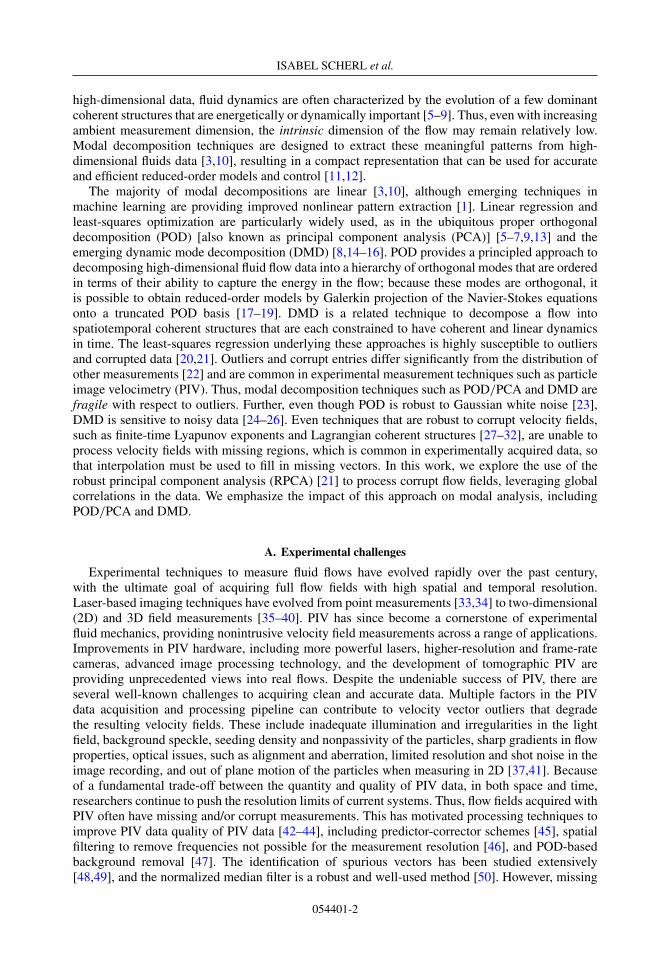
FIG. 1. Schematic of RPCA filtering applied to corrupt flow-field data. Corrupted snapshots are arrangedas column vectors in the matrix X, which is decomposed into the sum of a low-rank matrix L and a sparsematrix of outliers S.

vectors often cluster in regions of high shear, presenting a challenge for standard vector validationand interpolation methods that rely on local flow information [50]. In this work, we leverage robuststatistics and global spatiotemporal coherent structures across the entire data set to fill in missingmeasurements and improve modal decomposition of fluid flow fields.

B. Contributions of this work

We investigate the use of RPCA [21], a robust variant of POD/PCA [20,51]. RPCA uses asparsity-promoting optimization to decompose a data matrix into the sum of a low-rank matrixcontaining coherent structures and a sparse matrix containing outliers. RPCA was originallypopularized in the Netflix matrix completion algorithm for its recommender system [52] and hassince been widely used for image and video processing [53], electrical capacitance tomography[54], and voice separation [55]. Here, we use RPCA filtering to process flow-field data fromseveral simulations and experiments. Figure 1 demonstrates the ability of RPCA to uncoverand isolate the dominant low-rank coherent structures from sparse outliers in flow data froman idealized example. In addition to directly analyzing and processing flow-field data, we alsoperform PCA and DMD modal analyses on the data before and after RPCA filtering to assess itsperformance.

Here we consider a range of simulated and experimentally acquired flow fields of varyingcomplexity to isolate and analyze various aspects of the algorithm applied to data from fluidmechanics. First, we investigate high-fidelity flow fields from direct numerical simulations of alaminar flow past a cylinder and a turbulent channel flow, where it is possible to artificially addcorrupt velocity field vectors to compare the RPCA filtered fields with a known ground truth. Next,we apply the method to two experimentally acquired data sets, including a companion laminar flowpast a cylinder and measurements of a cross-flow turbine wake. Although there is not a ground-truthmodel for these flows, it is possible to estimate the effect of RPCA filtering in reducing outliers andcorruption by analyzing the DMD spectrum, which has well-stereotyped behavior for such periodicwake flows [24]. In all cases, we show that the RPCA filtered fields yield DMD spectra that aremore consistent with a periodic wake in the absence of noise.

This work is organized as follows: First, we present the standard POD/PCA and DMD modalanalysis techniques in Sec. II, followed by the RPCA method in Sec. III. Section IV describes thefour flow fields used in this analysis. Results of RPCA filtering on these flow fields and its impacton downstream modal analysis are presented in Sec. V.

054401-3

ISABEL SCHERL et al.

FIG. 2. Flowchart showing how we apply RPCA filtering to a data matrix and analyze the results.Depending on the data set in question, the data matrix may be artificially corrupted prior to RPCA filtering(Sec. IV). The results of principal component analysis and dynamic mode decomposition performed on the datamatrix (X) are referred to as PCA and DMD modes, respectively, whereas those same operations performed onthe low-rank matrix (L) are referred to as RPCA and RDMD modes.

II. MODAL ANALYSIS

Extracting coherent structures from high-dimensional data has been a central challenge in fluidmechanics for decades. Here we review two leading modal decomposition techniques for data fromfluid mechanics, the POD, also known as PCA (Sec. II A), and the DMD (Sec. II B). Both methodsapply equally well to data from simulations or experiments. We use these two modal decompositiontechniques to assess the effectiveness of RPCA filtering, in processing and correcting corrupt flowfields. Both techniques are based on the singular value decomposition (SVD) [56–59] and there areseveral detailed discussions of these decompositions [3,8,10,20]. The RPCA algorithm is explainedin Sec. III.

In this work, we follow the flowchart shown in Fig. 2. RPCA filtering is applied to a data matrix(X) which is bisected into the low-rank structure (L) and sparse (S) subspaces. From there, RPCAmodes and DMD modes are calculated from the low-rank data. We also calculate the POD/PCAand DMD modes on the data matrix.

A. Proper orthogonal decomposition

Proper orthogonal decomposition—referred to as PCA throughout results—is a widely usedmethod to identify spatially correlated coherent structures from data, decomposing the flow fieldinto a linear combination of orthogonal modes that are arranged hierarchically by energy content.There are several variants of POD [3,6,7,9,13,60], and we will present a variant of the snapshotPOD of Sirovich that relies on the numerically stable SVD [20,60]. First, flow-field data (e.g., avelocity or vorticity field) is measured or computed on a discrete spatial grid, and m snapshots ofthese flow fields are collected at various times t1, t2, . . . , tm. The flow-field data at time tk may bereshaped into a column vector xk = x(tk ) ∈ Rn, where n denotes the number of flow variables timesthe number of spatial grid locations. Next, a data matrix is formed by arranging the column vectorsxk in a matrix X:

X =⎡⎣

| | |x1 x2 · · · xm

| | |

⎤⎦. (1)

Finally, POD modes are obtained by computing the singular value decomposition of X ∈ Rn×m:

X = U�VT , (2)

where superscript T defines the matrix transpose, U ∈ Rn×n, � ∈ Rn×m, and V ∈ Rm×m. Thecolumns of U are POD modes with the same dimension as a flow field x. POD modes areorthonormal so that UT U = I; similarly, VT V = I. Moreover, the columns of U (respectively, rowsof VT ) are arranged in order of their importance in describing the data. The importance of each

054401-4

ROBUST PRINCIPAL COMPONENT ANALYSIS FOR MODAL …

mode (i.e., column of U) is given by the corresponding entry of the non-negative, diagonal matrixof singular values � ∈ Rn×m.

The matrix X will exhibit low-rank structure, so that it is well approximated by the first r �m < n columns of U and V:

X ≈ Ur�rVTr , (3)

where Ur and Vr denote the first r columns of each matrix and �r denotes the first r × r sub-blockof �. In fact, the Eckart-Young theorem states that this is the optimal rank-r approximation of thematrix X in a least-squares sense. More details about the SVD can be found in Ref. [20].

After truncating all but the first r dominant modes, a flow-field snapshot x may be approximatedby a linear combination of these modes:

x ≈r∑

k=1

ukαk,

where αk is the POD mode coefficient.Because the POD modal basis is orthogonal, it is possible to obtain a reduced-order nonlinear

dynamical system for the evolution of the coefficients αk (t ) in time via Galerkin projection of theNavier-Stokes equations onto the POD basis. In this way, the POD basis may be thought of a data-driven generalization of the Fourier basis that is tailored to a particular flow field. POD is also closelyrelated to PCA [51], the Karhunen-Loève decomposition [61], empirical orthogonal functions [62],or the Hotelling transform [63,64].

B. Dynamic mode decomposition

DMD is a modal decomposition technique that simultaneously identifies spatially coherentmodes that are constrained to have the same linear behavior in time, given by oscillations at afixed frequency with growth or decay [8,15]. Thus, the dynamic mode decomposition provides adimensionality reduction into a set of spatial modes along with a linear model for how these modesevolve in time. This is in contrast to POD, which results in orthogonal modes arranged in terms ofenergy content and without consideration of dynamics. However, in many formulations, DMD isclosely related to POD, and may be thought of as a linear combination of POD modes that resultsin linear evolution in time. DMD also has deep connections to nonlinear dynamical systems viaKoopman operator theory [8,14,16,65,66].

In the original formulation of DMD [15], the snapshots in the data matrix in Eq. (1) are spacedevenly in time, so that tk = k�t with �t sufficiently small to resolve the highest frequencies inthe dynamics. Generalizations have since been formulated to allow for nonsequential time series[16,67] and for data that is under-resolved in space [68,69] or time [70]; however, for simplicity, wewill present the standard exact DMD formulation of Tu et al. [16] with evenly spaced and sequentialsnapshots. DMD seeks to identify the leading eigenvalues and eigenvectors of the best-fit linearoperator A that evolves snapshots forward in time:

xk+1 ≈ Axk . (4)

The eigenvectors φ of A have the dimensions of a flow field and correspond to spatiotemporalcoherent structures whose dynamics in time evolve according to the associated eigenvalue γ .

In practice, this operator is identified by first splitting the data in Eq. (1) into two matrices:

X =⎡⎣

| | |x1 x2 · · · xm−1

| | |

⎤⎦ X′ =

⎡⎣

| | |x2 x3 · · · xm

| | |

⎤⎦, (5a)

and then solving for the best-fit operator that satisfies

X′ ≈ AX (6)

054401-5

ISABEL SCHERL et al.

via the following least-squares optimization problem:

A = argminA

||X′ − AX||F = X′X† ≈ X′Vr�−1r UT

r . (7)

Here we are minimizing the Frobenius norm || · ||F via the pseudoinverse X† = V�−1UT

≈ Vr�−1r UT

r .In practice, the matrix A is far too large to analyze directly, and instead, we project A onto an

r-dimensional POD subspace, given by the columns of Ur :

A = UTr AUr = UT

r X′Vr�−1r . (8)

The eigenvalues of A are the same as the eigenvalues of A, which are known as the DMDeigenvalues. They are computed via the eigendecomposition of the r × r matrix A:

AW = W�. (9)

Finally, the corresponding DMD modes are reconstructed using the full-dimensional data along withthe reduced eigenvectors in W:

� = X′Vr�−1r W. (10)

This formula for the eigenvectors is from the exact DMD algorithm [8,16]; the original formulationof Schmid [15] computes modes as � = UrW.

With the DMD modes � and eigenvalues � it is possible to reconstruct the state at time k�t ,

xk =r∑

j=1

φ jγk−1b j = ��k−1b, (11)

where the vector b of mode amplitudes is generally computed as

b = �†x1. (12)

More principled approaches to select the few dominant modes have been considered based onsparsity-promoting optimization [71].

The spectral expansion above may also be written in continuous time by introducing thecontinuous eigenvalues ω = log(γ )/�t :

x(t ) =r∑

j=1

φ jeω j t b j = � exp(�t )b, (13)

where � is a diagonal matrix containing the continuous-time eigenvalues ω j .DMD is known to be extremely sensitive to noisy data [24–26], and the eigenvalues specifically

suffer from a bias that is not reduced with increasing data. There are several modifications to makeDMD more robust to noise, including averaging forward-time and backward-time operators [25],total least squares [26], and variable projection [67]. For periodic wake data, as explored in threeof the examples in this paper, the discrete-time eigenvalues should occur in complex conjugatepairs γ , γ exactly on the unit circle in the complex plane for clean data. Similarly, the continuous-time eigenvalues should be in complex conjugate pairs ±iω on the imaginary axis, indicating pureoscillations with no growth or decay [24,72]. In Ref. [24], Bagheri characterized the perturbativeeffect of noise on these eigenvalues, deriving an asymptotic expression for how high frequencyeigenvalues become increasingly affected by noise. If the true continuous-time eigenvalue shouldbe ±iω in the absence of noise, Bagheri showed that in the presence of perturbative white noisewith magnitude ε � 1 the observed eigenvalue pair is

±iω − εCω2 + O(ε2), (14)

054401-6

ROBUST PRINCIPAL COMPONENT ANALYSIS FOR MODAL …

where C is a sensitivity constant. Thus, low noise levels cause a spurious real-valued damping−εCω2 that is quadratic in the frequency. We will make extensive use of this property to assess thequality of our RPCA filtered fields by computing the ratio of the best-fit factor εC before and afterapplying RPCA filtering. εC should decrease as a consequence of reduced noise and corruption.

III. ROBUST EXTRACTION OF FLUID COHERENT STRUCTURES

Techniques based on least-squares regression, such as POD/PCA and DMD, are highly sus-ceptible to outliers and corrupted data, making them fragile with respect to some experimentalmeasurement errors. Outliers and corruption are defined as data points that differ significantly fromthe statistical distribution of the majority of the data set [22], so that they cannot be considered as theoriginal data plus a small-to-moderate amount of white noise. To mitigate this sensitivity, Candeset al. [21] have developed RPCA that seeks to decompose a data matrix X into a structured low-rankmatrix L that is characterized by dominant coherent structures and a sparse matrix S containingoutliers and corrupt data:

X = L + S. (15)

The principal components of L are robust to outliers and corrupt data, which are isolated in S. Thisdecomposition, also referred to as a filter, has profound implications for many modern problems ofinterest, including video surveillance (where the background objects appear in L and foregroundobjects appear in S), facial recognition (eigenfaces are in L and shadows, occlusions, etc., are inS), natural language processing and latent semantic indexing, and ranking problems.1 StandardPCA/POD is effective at removing white noise that is smaller than the relevant singular valuesin the data [23]; however, it is not able to remove outliers. Instead, RPCA is used to correct outliersthat differ significantly from the distribution of the other observations.

Mathematically, the goal is to find L and S that satisfy the following:

minL,S

rank(L) + ||S||0 subject to L + S = X. (16)

||S||0 counts the number of nonzero elements in S, quantifying how sparse it is. rank(L) is thenumber of nonzero singular values in L, quantifying how many linearly independent rows andcolumns describe the data. However, neither the rank(L) nor the ||S||0 terms are convex, makingthis optimization intractable. Similarly to the compressed sensing problem, it is possible to solvefor L and S with high probability using a convex relaxation of (16):

minL,S

||L||∗ + λ0||S||1 subject to L + S = X, (17)

where || · ||∗ is the nuclear norm, given by the sum of singular values which is a proxy for therank of the matrix, and || · ||1 is the 1-norm of the matrix viewed as a vector, given by the sum ofthe magnitudes of each entry in the matrix, which is a proxy for the || · ||0 norm of a matrix; thehyperparameter λ0 is given by λ0 = λ/

√max(n, m). The solution to (17) converges to the solution

of (16) with high probability if λ = 1, where n and m are the dimensions of X, given that L is notsparse and S is not low rank. In the examples below, these assumptions may only be partially valid,so the optimal value of λ may vary slightly. The convex problem in (17) is known as principalcomponent pursuit and may be solved using the augmented Lagrange multiplier (ALM) algorithm.

1The ranking problem may be thought of in terms of the Netflix prize for matrix completion. In the Netflixprize, a large matrix of preferences is constructed, with rows corresponding to users and columns correspondingto movies. This matrix is sparse, as most users only rate a handful of movies. The Netflix prize seeks toaccurately fill in the missing entries of the matrix, revealing the likely user rating for movies the user has notseen.

054401-7

ISABEL SCHERL et al.

Specifically, an augmented Lagrangian may be constructed:

L(L, S, Y) = ||L||∗ + λ0||S||1 + 〈Y, X − L − S〉 + υ

2||X − L − S||2F , (18)

where Y is the matrix of Lagrange multipliers and υ is a hyperparameter. We then solve for Lk andSk to minimize L, update the Lagrange multipliers

Yk+1 = Yk + υ(X − Lk − Sk ),

and iterate until convergence. In this work, an inexact ALM implementation from Ref. [73] is used.The alternating directions method (ADM) [74,75] provides another simple procedure.

After the low-rank matrix L is obtained, it is possible to compute robust POD/PCA modes(Sec. II A) as in Eq. (2):

L = U�VT . (19)

Henceforth, we refer to the modes in U from L as RPCA modes. We note that in many flowapplications it is important to subtract the mean flow before computing POD, which allows the PODeigenvalues to be interpreted as the variance of fluctuations and the expansion to respect boundaryconditions by construction. However, before computing RPCA, it may be difficult to obtain anaccurate mean flow estimate. Instead, we advocate computing the RPCA, then subtracting the meanof L from itself, and finally computing POD on the mean-subtracted low-rank matrix; this final PODstep will remove small amounts of white noise.

Similarly, it is also possible to compute robust DMD (RDMD) modes and eigenvalues. We notethat the RDMD in this work should not be confused with the recursive DMD of Noack et al.[76], which uses the same acronym. We also note that this decomposition is similar in spirit to thecoherent vortex simulation approach [77], which separates turbulent flows into coherent and randomparts based on a wavelet decomposition. However, RPCA does not perform this decompositionusing a universal basis, such as wavelets, that rely on scale separation but rather based on statisticalcorrelations in the data.

IV. MODEL FLOWS

We demonstrate RPCA filtering on several example data sets of varying complexity, drawn fromdirect numerical simulations (DNS) and PIV data from experiments. Figure 3 provides an overviewof the four example flow fields.

A. Cylinder flow

Flow past a cylinder is a canonical example in fluid mechanics. We consider data from DNS ata diameter-based Reynolds number of 100 and from PIV measurements at Reynolds number 413[78].

The DNS data are generated by simulating the two-dimensional incompressible Navier-Stokesequations using the immersed boundary projection method [79,80]. The computational domaincomprises four nested grids: The finest grid covers a domain of 9 × 4 and the largest grid coversa domain of 72 × 32, where lengths are nondimensionalized by the cylinder diameter. Each gridcontains 449 × 199 points with a resolution of 50 points per cylinder diameter. The time step is�t = 0.02 and data are sampled at intervals of 10�t (30 times the vortex shedding frequency)with m = 150 snapshots saved, covering 5 vortex shedding cycles. The DNS provides a benchmark,where the uncorrupted flow field is known, to quantitatively assess performance of RPCA filteringon data with artificial salt-and-pepper corruption. Corrupted sample points are chosen uniformly inspace and time at a given rate, and both the u and v velocity components at each selected locationare randomly assigned a value of ±10 times the standard deviation of the streamwise velocity data.In addition, we consider a second case where corrupted sample points are chosen with a bias towardregions of high vorticity or shear magnitude, which is more physically realistic for PIV data. In this

054401-8

ROBUST PRINCIPAL COMPONENT ANALYSIS FOR MODAL …

FIG. 3. Left: Example flow-field data. Right: Singular value spectrum for each data set. Mean flow travelsfrom left to right in all cases.

second case, we select measurements for corruption based on a probability density given by α + |ω|,where α is a small positive constant and |ω| is the absolute value of the vorticity; when the rate ofcorruption is sufficiently high, these corrupted fields begin to resemble the uniformly corruptedcases, but with more corruption in vortex cores. Because vorticity is calculated from velocity fieldsusing a finite-difference derivative, there is a higher rate of corruption in the vorticity fields than inthe velocity fields.

The PIV data has frame size of 135 × 80 grid points with a resolution of 8 points per cylinderdiameter. Data are sampled at a rate of 20 Hz (125 times the shedding frequency) with m = 8000snapshots saved, which corresponds to 64 vortex shedding cycles.

B. Turbulent channel flow

For a more complex and multiscale flow, we consider DNS data from a forced, fully developedturbulent channel flow data with a friction velocity Reynolds number of Reτ = 1000, from theJohns Hopkins Turbulence Database [81]. This example provides a test case to see how turbulentkinetic energy at various scales is filtered depending on the level of added noise. The addition ofnoise is similar to the cylinder DNS where randomly selected sample points of the streamwiseand cross-stream velocity fields are assigned a value of ±10 standard deviations of the streamwisevelocity data. Due to the size of the full data set, we only consider two-dimensional fields on themidplane, with a 512 × 512 grid of three component velocity measurements spanning the channelwidth. Data are sampled at a rate of 966 times the mean flow-through time with m = 1000 snapshots.

C. Cross-flow turbine wake

Finally, we consider PIV wake data from a cross-flow turbine experiment conducted at theUniversity of Washington. Cross-flow turbines can be used to extract power from wind andwater currents for renewable energy generation. This flow exhibits both coherent and broadbandphenomena and provides a challenging test-case RPCA filtering. The frame consists of 158 × 98grid points, at a resolution of 99 points per rotor diameter. Data are sampled at a rate of 32 timesthe blade-pass frequency with m = 1000 snapshots. Vectors were calculated using a multigrid,multipass algorithm with adaptive image deformation [82]. Resulting vector fields were then

054401-9

ISABEL SCHERL et al.

FIG. 4. RPCA filtering removes noise and outliers in the flow past a cylinder (black circle), from DNS (left)with 10% of velocity field measurements corrupted with salt-and-pepper noise, and PIV measurements (right).All frames show resultant vorticity fields. As the parameter λ is decreased, RPCA filtering is more aggressive,eventually incorrectly identifying coherent flow structures as outliers.

validated using a normalized median filter with potential replacement by secondary correlationpeaks. The cross-correlation and validation steps result in missing data, particularly in regions ofhigh vorticity and shear. To apply RPCA filtering, these missing values are randomly assigneda value of ±10 standard deviations of the streamwise flow data, in contrast to the experimentalcylinder wake where missing measurements were previously interpolated.

V. RESULTS

We now explore the ability of RPCA filtering to isolate and remove noise and corruption fromthe example flow fields. We will begin with the simulated and experimental flow past a cylinder,followed by data from the Johns Hopkins turbulent channel flow simulation, and ending with theexperimental wake of a cross-flow turbine.

A. Cylinder flow

Figure 4 shows the results of RPCA filtering for flow past a cylinder, providing a side-by-sidecomparison of PIV and corrupted DNS data. Although the Reynolds numbers differ by a factor offour, the flow fields are qualitatively similar, characterized by periodic, laminar vortex shedding.For λ = 1, the data are correctly segmented with the coherent flow in L and the sparse corruptionin S. When λ is too small, RPCA filtering is overly aggressive, incorrectly including relevant flowstructures in S, and when λ is too large, the corruption is not filtered.

For the experimental data in Fig. 4 (right), the optimal value of λ is less clear. For λ = 0.1,the low-rank field L is visually smoother than the field at λ = 1, but the sparse matrix S containsa significant portion of the wake structures, indicating overfiltering. This filtering becomes morepronounced in the movies, where it is clear that much of the high-frequency “noise” in the bypassflow is actually free-stream turbulence, which is consistent with the turbulence intensity of the

054401-10

ROBUST PRINCIPAL COMPONENT ANALYSIS FOR MODAL …

FIG. 5. RPCA filtering removes vorticity-biased corruption from simulated flow past a cylinder at Reynoldsnumber 100. Unlike results shown in Fig. 4, corrupt entries are concentrated in regions of high vorticity insteadof being uniformly distributed. In the flow on the left, η = 1% of the velocity field measurements are corruptedand on the right η = 10% of the velocity field measurements are corrupted. All frames show resultant vorticityfields.

experiments. Further, as subsequently discussed, when we compute the RPCA modes, it is clearthat the λ = 0.1 case is heavily filtering out all but the first three modes. Thus, it appears thatthe theoretically optimal value λ = 1 has the best performance, although there may be a trade-offbetween filtering ambient free-stream turbulence and coherent structures of interest in experiments.

Figure 5 shows the results of RPCA filtering on the simulated data for the second case ofvorticity-biased corruption. Again, in all cases, the theoretically optimal value of λ = 1 yields thebest segmentation of the corruption into the matrix S. When the rate of corruption is increased from1% (left) to 10% (right), the free-stream flow begins to become corrupted, resembling the uniformcorruption case in Fig. 4. The mean error and relative nuclear norm of the low-rank matrix (L)compared to the true, uncorrupted data (X) are shown in Fig. 6 for varying percentages of corruptentries. Statistically, results are similar for vorticity-biased and randomly-distributed corruption.In both cases, RPCA filtering is remarkably robust to corruption, even for corruption in excess of

FIG. 6. Error (||Xuncorrupted − L||F/||Xuncorrupted||F ) and relative nuclear norm [||L||∗/||X ||∗= sum(σL )/sum(σX,uncorrupted )] of the low-rank matrix L compared with the uncorrupted data X forvarying percentages of corruption.

054401-11

ISABEL SCHERL et al.

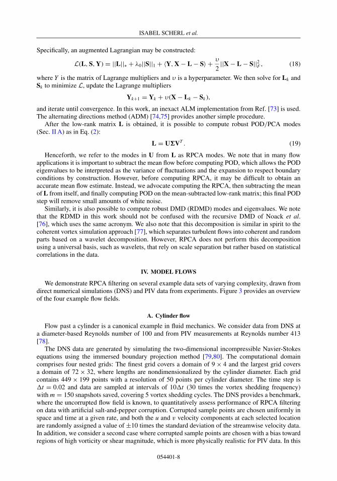
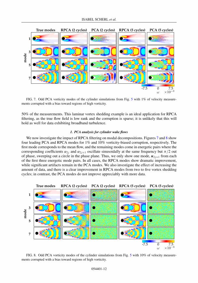
FIG. 7. Odd PCA vorticity modes of the cylinder simulations from Fig. 5 with 1% of velocity measure-ments corrupted with a bias toward regions of high vorticity.

50% of the measurements. This laminar vortex shedding example is an ideal application for RPCAfiltering, as the true flow field is low rank and the corruption is sparse; it is unlikely that this willhold as well for data exhibiting broadband turbulence.

1. PCA analysis for cylinder wake flows

We now investigate the impact of RPCA filtering on modal decompositions. Figures 7 and 8 showfour leading PCA and RPCA modes for 1% and 10% vorticity-biased corruption, respectively. Thefirst mode corresponds to the mean flow, and the remaining modes come in energetic pairs where thecorresponding coefficients α2 j and α2 j+1 oscillate sinusoidally at the same frequency but π/2 outof phase, sweeping out a circle in the phase plane. Thus, we only show one mode, u2 j+1 from eachof the first three energetic mode pairs. In all cases, the RPCA modes show dramatic improvement,while significant artifacts remain in the PCA modes. We also investigate the effect of increasing theamount of data, and there is a clear improvement in RPCA modes from two to five vortex sheddingcycles; in contrast, the PCA modes do not improve appreciably with more data.

FIG. 8. Odd PCA vorticity modes of the cylinder simulations from Fig. 5 with 10% of velocity measure-ments corrupted with a bias toward regions of high vorticity.

054401-12

ROBUST PRINCIPAL COMPONENT ANALYSIS FOR MODAL …

FIG. 9. L2 error between the true PCA modes of the clean cylinder simulation data X and the RPCA andPCA modes for corrupted data with 1% (left) and 10% (right) vorticity-biased corruption.

To quantify the improvement observed above, we compute the L2 error between the PCA andRPCA modes of corrupted data and the PCA modes for the clean data (i.e., DNS results) as afunction of the number of shedding periods. As shown in Fig. 9, the RPCA mode velocity fieldsquickly converge to a small error as the amount of data is increased for both the 1% and 10%corruption cases, while the PCA modes converge much more slowly and still have considerableerror after five shedding periods are included in the analysis.

The modes for the PIV data for the cylinder flow are shown in Fig. 10. This figure highlights theeffect of λ, the sparsity hyperparameter, which was previously discussed with respect to Fig. 4. Inthis case, we do not have a clean ground-truth data set to compare against. Although the flow fieldin Fig. 4 appears to have less corruption for λ = 0.1, here we see that all RPCA modes after the firstthree modes are heavily filtered, as seen in the rapid drop off in the singular values after the thirdmode. The corresponding modes are highly corrupt, further supporting that λ = 0.1 is not a goodchoice. In contrast, the RPCA modes for the theoretically optimal λ = 1 case appear to have slightlyless free-stream corruption than the PCA modes. Also, as expected, for a large enough value of λ,the RPCA filtering has little effect on the modes.

FIG. 10. Odd PCA vorticity modes of the experimental cylinder data for PCA and RPCA at λ = 0.1, 1,

and 10, along with their singular values.

054401-13

ISABEL SCHERL et al.

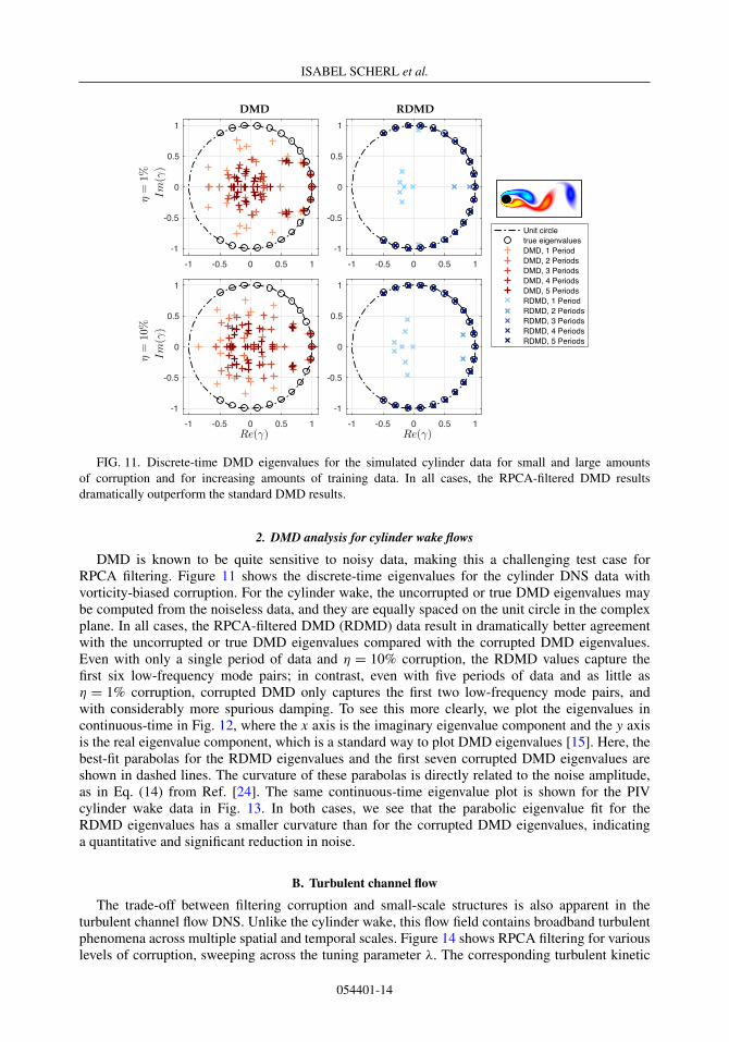
FIG. 11. Discrete-time DMD eigenvalues for the simulated cylinder data for small and large amountsof corruption and for increasing amounts of training data. In all cases, the RPCA-filtered DMD resultsdramatically outperform the standard DMD results.

2. DMD analysis for cylinder wake flows

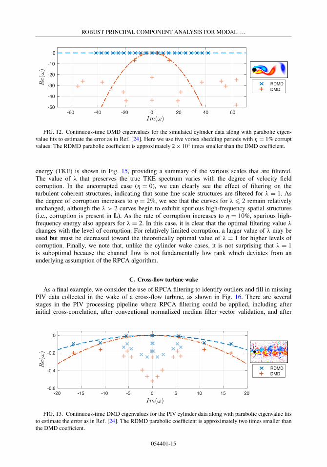
DMD is known to be quite sensitive to noisy data, making this a challenging test case forRPCA filtering. Figure 11 shows the discrete-time eigenvalues for the cylinder DNS data withvorticity-biased corruption. For the cylinder wake, the uncorrupted or true DMD eigenvalues maybe computed from the noiseless data, and they are equally spaced on the unit circle in the complexplane. In all cases, the RPCA-filtered DMD (RDMD) data result in dramatically better agreementwith the uncorrupted or true DMD eigenvalues compared with the corrupted DMD eigenvalues.Even with only a single period of data and η = 10% corruption, the RDMD values capture thefirst six low-frequency mode pairs; in contrast, even with five periods of data and as little asη = 1% corruption, corrupted DMD only captures the first two low-frequency mode pairs, andwith considerably more spurious damping. To see this more clearly, we plot the eigenvalues incontinuous-time in Fig. 12, where the x axis is the imaginary eigenvalue component and the y axisis the real eigenvalue component, which is a standard way to plot DMD eigenvalues [15]. Here, thebest-fit parabolas for the RDMD eigenvalues and the first seven corrupted DMD eigenvalues areshown in dashed lines. The curvature of these parabolas is directly related to the noise amplitude,as in Eq. (14) from Ref. [24]. The same continuous-time eigenvalue plot is shown for the PIVcylinder wake data in Fig. 13. In both cases, we see that the parabolic eigenvalue fit for theRDMD eigenvalues has a smaller curvature than for the corrupted DMD eigenvalues, indicatinga quantitative and significant reduction in noise.

B. Turbulent channel flow

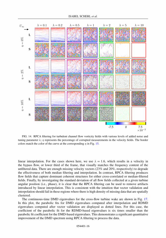
The trade-off between filtering corruption and small-scale structures is also apparent in theturbulent channel flow DNS. Unlike the cylinder wake, this flow field contains broadband turbulentphenomena across multiple spatial and temporal scales. Figure 14 shows RPCA filtering for variouslevels of corruption, sweeping across the tuning parameter λ. The corresponding turbulent kinetic

054401-14

ROBUST PRINCIPAL COMPONENT ANALYSIS FOR MODAL …

FIG. 12. Continuous-time DMD eigenvalues for the simulated cylinder data along with parabolic eigen-value fits to estimate the error as in Ref. [24]. Here we use five vortex shedding periods with η = 1% corruptvalues. The RDMD parabolic coefficient is approximately 2 × 104 times smaller than the DMD coefficient.

energy (TKE) is shown in Fig. 15, providing a summary of the various scales that are filtered.The value of λ that preserves the true TKE spectrum varies with the degree of velocity fieldcorruption. In the uncorrupted case (η = 0), we can clearly see the effect of filtering on theturbulent coherent structures, indicating that some fine-scale structures are filtered for λ = 1. Asthe degree of corruption increases to η = 2%, we see that the curves for λ � 2 remain relativelyunchanged, although the λ > 2 curves begin to exhibit spurious high-frequency spatial structures(i.e., corruption is present in L). As the rate of corruption increases to η = 10%, spurious high-frequency energy also appears for λ = 2. In this case, it is clear that the optimal filtering value λ

changes with the level of corruption. For relatively limited corruption, a larger value of λ may beused but must be decreased toward the theoretically optimal value of λ = 1 for higher levels ofcorruption. Finally, we note that, unlike the cylinder wake cases, it is not surprising that λ = 1is suboptimal because the channel flow is not fundamentally low rank which deviates from anunderlying assumption of the RPCA algorithm.

C. Cross-flow turbine wake

As a final example, we consider the use of RPCA filtering to identify outliers and fill in missingPIV data collected in the wake of a cross-flow turbine, as shown in Fig. 16. There are severalstages in the PIV processing pipeline where RPCA filtering could be applied, including afterinitial cross-correlation, after conventional normalized median filter vector validation, and after

FIG. 13. Continuous-time DMD eigenvalues for the PIV cylinder data along with parabolic eigenvalue fitsto estimate the error as in Ref. [24]. The RDMD parabolic coefficient is approximately two times smaller thanthe DMD coefficient.

054401-15

ISABEL SCHERL et al.

FIG. 14. RPCA filtering for turbulent channel flow vorticity fields with various levels of added noise andtuning parameter λ; η represents the percentage of corrupted measurements in the velocity fields. The bordercolors match the color of the curve at the corresponding η in Fig. 15.

linear interpolation. For the cases shown here, we use λ = 1.6, which results in a velocity inthe bypass flow, or lower third of the frame, that visually matches the frequency content of theunfiltered data. There are enough missing velocity vectors (23% and 20%, respectively) to degradethe effectiveness of both median filtering and interpolation. In contrast, RPCA filtering producesflow fields that capture dominant coherent structures for either cross-correlated or median-filteredfields. Finally, by investigating the standard deviation of all flow fields collected at a given turbineangular position (i.e., phase), it is clear that the RPCA filtering can be used to remove artifactsintroduced by linear interpolation. This is consistent with the intuition that vector validation andinterpolation should fail in these regions where there is high density of missing data that are spatiallyclustered.

The continuous-time DMD eigenvalues for the cross-flow turbine wake are shown in Fig. 17.In this plot, the parabolic fits for DMD eigenvalues computed after interpolation and RDMDeigenvalues computed after vector validation are displayed as dotted lines. For this case, thecoefficient of the parabolic fit for the RDMD-based eigenvalues is six times smaller than theparabolic fit coefficient for the DMD-based eigenvalues. This demonstrates a significant quantitativeimprovement of the DMD spectrum using RPCA filtering to process the data.

054401-16

ROBUST PRINCIPAL COMPONENT ANALYSIS FOR MODAL …

FIG. 15. TKE spectra for various levels of corruption and RPCA filtering. The TKE profiles provide asummary of the filtering that occurs at various scales. As corruption increases, the filtering remove more high-frequency information.

FIG. 16. RPCA filtering of cross-flow turbine wake PIV data. The standard PIV processing pipeline(top row) includes several steps where RPCA filtering can be applied (bottom row). In the cross-correlatedstreamwise velocity field (top left), 23% of the velocity vectors are missing. Vector validation reduces themissing vectors to 20%. Finally, linear interpolation is used to fill in these missing vectors. In all cases, RPCAfiltering captures the relevant phase-averaged coherent structures with fewer outliers and missing data, whichappear as dark spots in the standard deviation plot.

FIG. 17. Continuous-time DMD eigenvalues for the turbine wake PIV data, along with parabolic eigen-value fits to estimate the error as in Ref. [24]. The RDMD parabolic coefficient is approximately six timessmaller than the DMD coefficient.

054401-17

ISABEL SCHERL et al.

VI. CONCLUSIONS AND DISCUSSION

In this work, we have demonstrated the ability of RPCA filtering to effectively recoverdominant coherent structures from corrupt flow fields with missing measurements. Unlike standardPOD/PCA, which is based on least squares and is susceptible to outliers and corruption, RPCAutilizes sparse optimization to separate a data matrix into a low-rank matrix containing correlatedstructures and a sparse matrix containing the spurious entries.

We apply RPCA filtering to several types of fluid flow data (DNS and PIV), ranging from laminarvortex shedding behind a circular cylinder, to fully turbulent channel flow DNS, and concluding withan experimental flow past a cross-flow turbine. These flows exhibit a variety of phenomena and arange of measurement quality. The DNS examples provide us with a baseline, where it is possible toadd corruption to quantitatively assess the performance of RPCA. For flow past a cylinder in DNS,RPCA filtering is extremely effective at separating the true flow field from considerable corruption,with robust recovery even in flow fields with excess of 50% of the measurements corrupted. Inthe experimental counterpart, RPCA is still able to remove large outliers and corruption, althoughthere is a trade-off between filtering the background turbulence and coherent structures in thewake. The fully turbulent channel flow DNS provides an opportunity to more fully explore thistrade-off in a controlled setting, where we can incrementally increase the corruption ratio andobserve the filtering effects on various spatial frequencies. As expected, an increasingly aggressivefiltering leads to degradation at higher wave numbers, although dominant coherent structures arerobustly preserved. Finally, the wake behind a cross-flow turbine provides a practical real-worldflow that directly benefits from improved PIV processing. In all three wake flows we also assess theperformance of RPCA filtering to yield more accurate modal decompositions. Although we do nothave ground-truth measurements and modal decompositions, except in the case of direct numericalsimulations, we know that continuous-time DMD eigenvalues should be arranged on the imaginaryaxis in the complex plane for clean data, and deviations from this may be quantified using thederivation from Bagheri [24]. In all three cases, we see considerable reduction in spurious damping,indicating the denoising effectiveness of RPCA. Based on these results, we believe that RPCA canbe a valuable algorithm in the arsenal of PIV processing and filtering techniques, particularly whenthe processing pipeline culminates in modal analysis.

There are a number of future directions motivated by this work. First, RPCA depends onthe hyperparameter λ, and a better understanding of how to objectively choose λ for differentconditions is important. Because RPCA is based on sparse, nonconvex optimization, it is alsolikely that improved optimization techniques may improve speed and robustness. Although thiswork considered three-dimensional flows, the data comprised two-dimensional cross sections, andthe current analysis could be extended to flow volumes. In principle, the RPCA method shouldgeneralize, although there may be computational scaling challenges. Recent results have extendedRPCA from linear subspaces to manifolds [83], so it may be possible to robustly characterize fluidsdata that is well described by a low-dimensional manifold [84], rather than a low-dimensional PODsubspace. Nonstationary flows may be more challenging for this method, as the bulk distributionwill drift. Similarly shocks may be erroneously flagged as outliers; however, this may providean opportunity to identify shocks in the data. Investigating these flows is an important avenue offuture work. It would also be useful to extend this work to PIV measurements of other turbineconfigurations [85]. Finally, the quality of the RPCA filtered flow fields for additional downstreamanalyses should be assessed for example, in dynamical systems modeling via Galerkin projection[19] or regression [18] onto the filtered modes and in control [86].

The code and videos for this work are available [87,88].

054401-18

ROBUST PRINCIPAL COMPONENT ANALYSIS FOR MODAL …

ACKNOWLEDGMENTS

We gratefully acknowledge funding from the Army Research Office (Grant No. ARO W911NF-19-1-0045) and Naval Facilities Engineering Command. We also thank Jared Callaham, NathanKutz, Kazuki Maeda, and Joshua Proctor for valuable discussions.

[1] S. L. Brunton, B. R. Noack, and P. Koumoutsakos, Machine learning for fluid mechanics, Annu. Rev.Fluid Mech. 52, 477 (2020).

[2] K. Duraisamy, G. Iaccarino, and H. Xiao, Turbulence modeling in the age of data, Annu. Rev. Fluid Mech.51, 357 (2019).

[3] K. Taira, S. L. Brunton, S. T. M. Dawson, C. W. Rowley, T. Colonius, B. J. McKeon, O. T. Schmidt, S.Gordeyev, V. Theofilis, and L. S. Ukeiley, Modal analysis of fluid flows: An overview, AIAA J. 55, 4013(2017).

[4] A. Pollard, L. Castillo, L. Danaila, and M. Glauser, Whither Turbulence and Big Data in the 21st Century?(Springer, Berlin, 2016).

[5] N. Aubry, P. Holmes, J. L. Lumley, and E. Stone, The dynamics of coherent structures in the wall regionof a turbulent boundary layer, J. Fluid Mech. 192, 115 (1988).

[6] G. Berkooz, P. Holmes, and J. L. Lumley, The proper orthogonal decomposition in the analysis ofturbulent flows, Annu. Rev. Fluid Mech. 25, 539 (1993).

[7] P. J. Holmes, J. L. Lumley, G. Berkooz, and C. W. Rowley, Turbulence, Coherent Structures, DynamicalSystems and Symmetry, Cambridge Monographs in Mechanics, 2nd ed. (Cambridge University Press,Cambridge, UK, 2012).

[8] J. N. Kutz, S. L. Brunton, B. W. Brunton, and J. L. Proctor, Dynamic Mode Decomposition: Data-DrivenModeling of Complex Systems (SIAM, Philadelphia, PA, 2016).

[9] J. L. Lumley, Stochastic Tools in Turbulence (Academic Press, New York, 1970).[10] K. Taira, M. S. Hemati, S. L. Brunton, Y. Sun, K. Duraisamy, S. Bagheri, S. Dawson, and C.-A. Yeh,

Modal analysis of fluid flows: Applications and outlook, arXiv:1903.05750.[11] S. L. Brunton and B. R. Noack, Closed-loop turbulence control: Progress and challenges, Appl. Mech.

Rev. 67, 050801 (2015).[12] C. W. Rowley and S. T. M. Dawson, Model reduction for flow analysis and control, Annu. Rev. Fluid

Mech. 49, 387 (2017).[13] A. Towne, O. T. Schmidt, and T. Colonius, Spectral proper orthogonal decomposition and its relationship

to dynamic mode decomposition and resolvent analysis, J. Fluid Mech. 847, 821 (2018).[14] C. W. Rowley, I. Mezic, S. Bagheri, P. Schlatter, and D. S. Henningson, Spectral analysis of nonlinear

flows, J. Fluid Mech. 641, 115 (2009).[15] P. J. Schmid, Dynamic mode decomposition of numerical and experimental data, J. Fluid Mech. 656, 5

(2010).[16] J. H. Tu, C. W. Rowley, D. M. Luchtenburg, S. L. Brunton, and J. N. Kutz, On dynamic mode

decomposition: Theory and applications, J. Comput. Dyn. 1, 391 (2014).[17] K. Carlberg, M. Barone, and H. Antil, Galerkin v. least-squares petrov–galerkin projection in nonlinear

model reduction, J. Comput. Phys. 330, 693 (2017).[18] J.-C. Loiseau and S. L. Brunton, Constrained sparse Galerkin regression, J. Fluid Mech. 838, 42 (2018).[19] B. R. Noack, K. Afanasiev, M. Morzynski, G. Tadmor, and F. Thiele, A hierarchy of low-dimensional

models for the transient and post-transient cylinder wake, J. Fluid Mech. 497, 335 (2003).[20] S. L. Brunton and J. N. Kutz, Data-Driven Science and Engineering: Machine Learning, Dynamical

Systems, and Control (Cambridge University Press, Cambridge, UK, 2019).[21] E. J. Candès, X. Li, Y. Ma, and J. Wright, Robust principal component analysis? J. ACM 58, 11 (2011).[22] F. E. Grubbs, Procedures for detecting outlying observations in samples, Technometrics 11, 1 (1969).[23] M. Gavish and D. L. Donoho, The optimal hard threshold for singular values is 4/

√3, IEEE Trans. Inf.

Theory 60, 5040 (2014).

054401-19

ISABEL SCHERL et al.

[24] S. Bagheri, Effects of weak noise on oscillating flows: Linking quality factor, Floquet modes, andKoopman spectrum, Phys. Fluids 26, 094104 (2014).

[25] S. T. M. Dawson, M. S. Hemati, M. O. Williams, and C. W. Rowley, Characterizing and correcting forthe effect of sensor noise in the dynamic mode decomposition, Exp. Fluids 57, 42 (2016).

[26] M. S. Hemati, C. W. Rowley, E. A. Deem, and L. N. Cattafesta, De-biasing the dynamic modedecomposition for applied Koopman spectral analysis, Theor. Comput. Fluid Dyn. 31, 349 (2017).

[27] M. Farazmand and G. Haller, Computing Lagrangian coherent structures from their variational theory,Chaos 22, 013128 (2012).

[28] M. A. Green, C. W. Rowley, and A. J. Smits, The unsteady three-dimensional wake produced by atrapezoidal pitching panel, J. Fluid Mech. 685, 117 (2011).

[29] G. Haller, Lagrangian coherent structures from approximate velocity data, Phys. Fluids 14, 1851 (2002).[30] S. G. Raben, S. D. Ross, and P. P. Vlachos, Computation of finite-time Lyapunov exponents from time-

resolved particle image velocimetry data, Exp. Fluids 55, 1638 (2014).[31] S. C. Shadden, K. Katija, M. Rosenfeld, J. E. Marsden, and J. O. Dabiri, Transport and stirring induced

by vortex formation, J. Fluid Mech. 593, 315 (2007).[32] S. C. Shadden, F. Lekien, and J. E. Marsden, Definition and properties of Lagrangian coherent structures

from finite-time Lyapunov exponents in two-dimensional aperiodic flows, Physica D 212, 271 (2005).[33] J. W. Foreman Jr, E. W. George, and R. D. Lewis, Measurement of localized flow velocities in gases with

a laser doppler flowmeter, Appl. Phys. Lett. 7, 77 (1965).[34] Y. Yeh and H. Z. Cummins, Localized fluid flow measurements with an he–ne laser spectrometer,

Appl. Phys. Lett. 4, 176 (1964).[35] R. J. Adrian, Particle-imaging techniques for experimental fluid mechanics, Annu. Rev. Fluid Mech. 23,

261 (1991).[36] R. J. Adrian, Twenty years of particle image velocimetry, Exp. Fluids 39, 159 (2005).[37] R. J. Adrian and J. Westerweel, Particle Image Velocimetry (Cambridge University Press, Cambridge,

UK, 2011), Vol. 30.[38] M. Raffel, C. E. Willert, F. Scarano, C. J. Kähler, S. T. Wereley, and J. Kompenhans, Particle Image

Velocimetry: A Practical Guide (Springer, Berlin, 2018).[39] J. Westerweel, G. E. Elsinga, and R. J. Adrian, Particle image velocimetry for complex and turbulent

flows, Annu. Rev. Fluid Mech. 45, 409 (2013).[40] C. E. Willert and M. Gharib, Digital particle image velocimetry, Exp. Fluids 10, 181 (1991).[41] H. Huang, D. Dabiri, and M. Gharib, On errors of digital particle image velocimetry, Meas. Sci. Technol.

8, 1427 (1997).[42] D. Garcia, A fast all-in-one method for automated post-processing of PIV data, Exp. Fluids 50, 1247

(2011).[43] D. P. Hart, PIV error correction, Exp. Fluids 29, 13 (2000).[44] J. Nogueira, A. Lecuona, and P. A. Rodriguez, Data validation, false vectors correction and derived

magnitudes calculation on PIV data, Meas. Sci. Tech. 8, 1493 (1997).[45] F. F. J. Schrijer and F. Scarano, Effect of predictor–corrector filtering on the stability and spatial resolution

of iterative PIV interrogation, Exp. Fluids 45, 927 (2008).[46] S. Discetti, A. Natale, and T. Astarita, Spatial filtering improved tomographic PIV, Exp. Fluids 54, 1505

(2013).[47] M. A. Mendez, M. Raiola, A. Masullo, S. Discetti, A. Ianiro, R. Theunissen, and J.-M. Buchlin, Pod-based

background removal for particle image velocimetry, Exp. Therm. Fluid Sci. 80, 181 (2017).[48] J. Duncan, D. Dabiri, J. Hove, and 1, Universal outlier detection for particle image velocimetry (PIV) and

particle tracking velocimetry (PTV) data, Meas. Sci. Technol. 21, 057002 (2010).[49] J. Westerweel, Efficient detection of spurious vectors in particle image velocimetry data, Exp. Fluids 16,

236 (1994).[50] J. Westerweel and F. Scarano, Universal outlier detection for PIV data, Exp. Fluids 39, 1096 (2005).[51] K. Pearson, On lines and planes of closest fit to systems of points in space, Philos. Mag. 2, 559 (1901).[52] J. Wong, C. Colburn, E. Meeks, and S. Vedaraman, RAD–outlier detection on big data, 2015.

054401-20

ROBUST PRINCIPAL COMPONENT ANALYSIS FOR MODAL …

[53] T. Bouwmans and E. H. Zahzah, Robust PCA via principal component pursuit: A review for a comparativeevaluation in video surveillance, Comp. Vis. Image Under. 122, 22 (2014).

[54] J. Lei, S. Liu, X. Wang, and Q. Liu, An image reconstruction algorithm for electrical capacitancetomography based on robust principle component analysis, Sensors 13, 2076 (2013).

[55] P.-S. Huang, S. Deeann Chen, P. Smaragdis, and M. Hasegawa-Johnson, Singing-voice separation frommonaural recordings using robust principal component analysis, in Proceedings of the IEEE ICASSP,(IEEE, Los Alamitos, CA, 2012), p. 57–60.

[56] P. A. Businger and G. H. Golub, Algorithm 358: Singular value decomposition of a complex matrix[f1, 4, 5], Commun. ACM 12, 564 (1969).

[57] G. Golub and W. Kahan, Calculating the singular values and pseudo-inverse of a matrix, J. Soc. Ind. Appl.Math., Ser. B 2, 205 (1965).

[58] G. H. Golub and C. Reinsch, Singular value decomposition and least squares solutions, Numer. Math. 14,403 (1970).

[59] G. H. Golub and C. F. Van Loan, An analysis of the total least squares problem, SIAM J. Numer. Anal.17, 883 (1980).

[60] L. Sirovich, Turbulence and the dynamics of coherent structures, parts I-III, Q. Appl. Math. 45, 561(1987).

[61] K. Karhunen, Über lineare Methoden in der Wahrscheinlichkeitsrechnung, Vol. 37, Annales Academiæ-Scientiarum Fennicæ, Ser. A. I (Academia Scientiarum Fennica, Helsinki, 1947).

[62] E. N. Lorenz, Empirical orthogonal functions and statistical weather prediction, Technical Report,Massachusetts Institute of Technology (1956).

[63] H. Hotelling, Analysis of a complex of statistical variables into principal components, Journal ofEducational Psychology 24, 417 (1933).

[64] H. Hotelling, Analysis of a complex of statistical variables into principal components, Journal ofEducational Psychology 24, 498 (1933).

[65] I. Mezic, Spectral properties of dynamical systems, model reduction and decompositions, Nonlin. Dynam.41, 309 (2005).

[66] I. Mezic, Analysis of fluid flows via spectral properties of the Koopman operator, Annu. Rev. Fluid Mech.45, 357 (2013).

[67] T. Askham and J. N. Kutz, Variable projection methods for an optimized dynamic mode decomposition,SIAM J. Appl. Dyn. Syst. 17, 380 (2018).

[68] S. L. Brunton, J. L. Proctor, J. H. Tu, and J. N. Kutz, Compressed sensing and dynamic modedecomposition, J. Comput. Dyn. 2, 165 (2015).

[69] F. Gueniat, L. Mathelin, and L. Pastur, A dynamic mode decomposition approach for large and arbitrarilysampled systems, Phys. Fluids 27, 025113 (2015).

[70] J. H. Tu, C. W. Rowley, J. N. Kutz, and J. K. Shang, Spectral analysis of fluid flows using sub-Nyquist-ratePIV data, Exp. Fluids 55, 1805 (2014).

[71] M. R. Jovanovic, P. J. Schmid, and J. W. Nichols, Sparsity-promoting dynamic mode decomposition,Phys. Fluids 26, 024103 (2014).

[72] S. Bagheri, Koopman-mode decomposition of the cylinder wake, J. Fluid Mech. 726, 596 (2013).[73] A. Sobral, T. Bouwmans, and El-hadi Zahzah, Lrslibrary: Low-rank and sparse tools for background

modeling and subtraction in videos, in Robust Low-Rank and Sparse Matrix Decomposition: Applicationsin Image and Video Processing (CRC Press, Boca Raton, FL, 2015).

[74] Z. Lin, M. Chen, and Yi Ma, The augmented lagrange multiplier method for exact recovery of corruptedlow-rank matrices, arXiv:1009.5055.

[75] X. Yuan and J. Yang, Sparse and low-rank matrix decomposition via alternating direction methods(unpublished).

[76] B. R. Noack, W. Stankiewicz, M. Morzynski, and P. J. Schmid, Recursive dynamic mode decompositionof a transient cylinder wake, J. Fluid Mech. 809, 843 (2016).

[77] M. Farge and K. Schneider, Coherent vortex simulation (CVS), a semi-deterministic turbulence modelusing wavelets, Flow, Turbul. Combust. 66, 393 (2001).

054401-21

ISABEL SCHERL et al.

[78] J. K. Shang, Flexibility and curvature effects on vortex dynamics and fluid-structure interactions, Ph.D.thesis, Princeton University, 2015.

[79] T. Colonius and K. Taira, A fast immersed boundary method using a nullspace approach and multi-domainfar-field boundary conditions, Comput. Methods Appl. Mech. Eng. 197, 2131 (2008).

[80] K. Taira and T. Colonius, The immersed boundary method: A projection approach, J. Comput. Phys. 225,2118 (2007).

[81] J. Graham, K. Kanov, X. I. A. Yang, M. Lee, N. Malaya, C. C. Lalescu, R. Burns, G. Eyink, A. Szalay,R. D. Moser, and C. Meneveau, A web services accessible database of turbulent channel flow and its usefor testing a new integral wall model for LES, J. Turbul. 17, 181 (2016).

[82] F. Scarano, Iterative image deformation methods in PIV, Meas. Sci. Tech. 13, R1 (2001).[83] He Lyu, N. Sha, S. Qin, M. Yan, Y. Xie, and R. Wang, Manifold denoising by nonlinear robust principal

component analysis, in Advances in Neural Information Processing Systems (2019), pp. 13390–13400.[84] J.-C. Loiseau, B. R. Noack, and S. L. Brunton, Sparse reduced-order modeling: Sensor-based dynamics

to full-state estimation, J. Fluid Mech. 844, 459 (2018).[85] A. Posa, C. M. Parker, M. C. Leftwich, and E. Balaras, Wake structure of a single vertical axis wind

turbine, Int. J. Heat Fluid Flow 61, 75 (2016).[86] Z. P. Berger, P. R. Shea, M. G. Berry, B. R. Noack, S. Gogineni, and M. N. Glauser, Active flow control

for high speed jets with large window piv, Flow, Turbul. Combust. 94, 97 (2015).[87] Matlab code: github.com/ischerl/RPCA-PIV.[88] Videos: tinyurl.com/RPCA-PIV.

054401-22