Pi i l f C i i Principles of Communications

P i i l f C i iPrinciples of Communications

Chapter 3: Analog Modulation(continued)

Textbook: Ch 3, Ch 4.1-4.4, Ch 6.1-6.2

1

3 2 Eff t f N i AM S t3.2 Effect of Noise on AM SystemsBaseband system (a basis for comparison of various modulation systems):

No carrier demodulationNo carrier demodulationThe receiver is an ideal LPF with bandwidth W Noise power at the output of the receiverNoise power at the output of the receiver

0

002

W

n W

NP df N W−

= =∫Baseband SNR is given by

n(t)

2

0

R

b

PSN N W

⎛ ⎞ =⎜ ⎟⎝ ⎠

+ LPF

n(t)

)(tsm

2010/2011 Meixia Tao @ SJTU 2

+ LPF

E lExample:Find the SNR in a baseband system with a bandwidth of 5 kHz and with W/Hz. The transmitter power is 1kW and the channel attenuation is

140 / 2 10N −=

1210−power is 1kW and the channel attenuation is

Solution:

1210

12 3 9Solution: 12 3 910 10 10 WattsRP − −= × =

910 20RPS −⎛ ⎞⎜ ⎟ 14

0

2010 5000

R

bN N W −

⎛ ⎞ = = =⎜ ⎟ ×⎝ ⎠

1010log 20 13dB= =


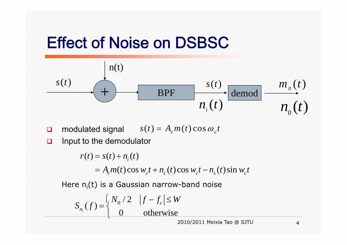
Eff t f N i DSBSCEffect of Noise on DSBSC n(t)

+ BPF demod

n(t)

( )s t )(0 tm( )s t+ BPF demod

)(tni )(0 tnmodulated signal Input to the demodulator

( ) ( ) cosc cs t A m t tω=

( ) ( ) ( )( ) cos ( )cos ( )sin

i

c c c c s c

r t s t n tA m t w t n t w t n t w t

= +

= + −

Here ni(t) is a Gaussian narrow-band noise

0 / 2( ) cN f f W

S f⎧ − ≤

= ⎨


( )0 otherwiseinS f = ⎨

⎩

In the demodulator, the received signal is first multiplied by a locally generated sinusoid signal

( ) cos( ) ( )cos cos( )( ) cos cos( ) ( )sin cos( )

c c c c

c c c s c c

r t w t A m t w t w tn t w t w t n t w t w t

φ φφ φ

+ = +

+ + − +

1 1( )cos ( )cos(2 )2 2c c cA m t A m t w tφ φ= + +

[ ]1 ( )cos ( )sin21

c sn t n tφ φ+ +

Assume coherent detector we have

[ ]1 ( )cos(2 ) ( )sin(2 )2 c c s cn t w t n t w tφ φ+ + − +

0φ2010/2011 Meixia Tao @ SJTU

Assume coherent detector, we have5

0φ =

Then the signal is passed through a LPF with bandwidth WThen the signal is passed through a LPF with bandwidth W

[ ]1( ) ( ) ( )2 c cy t A m t n t= + ( ) ( ) ( )

c i in n c n cS f S f f S f f

for f W

= − + +

≤where

The output SNR can thus be defined as2

21 A PP A PS⎛ ⎞

for f W≤

2

0

41 24

oc

c mo c m

o nn

A PP A PSN P WNP

⎛ ⎞ = = =⎜ ⎟⎝ ⎠

2A PSince the received power of DSBSC in baseband is The output SNR can be rewritten as

42

c mR

A PP =

0

R

oDSB b

PS SN WN N

⎛ ⎞ ⎛ ⎞= =⎜ ⎟ ⎜ ⎟⎝ ⎠ ⎝ ⎠

DBSSC does not provide any SNR improvement over a simple baseband systems


0oDSB b⎝ ⎠ ⎝ ⎠ simple baseband systems

Eff t f N i SSBEffect of Noise on SSBModulated signal:Input to the demodulator

( ) ( ) cos ( )sinc c c cs t A m t w t A m t w t= ± )

0 / 2 / 2( ) cN f f W

S f⎧ − ≤⎨

[ ] [ ]( ) ( ) cos ( ) ( ) sinA m t n t w t A m t n t w t= + + ± −)

0( )0 otherwise

cn

f fS f = ⎨

⎩( ) ( ) ( )ir t s t n t= + where

Output of LPF:

[ ] [ ]( ) ( ) cos ( ) ( ) sinc c c c s cA m t n t w t A m t n t w t= + + ±

1( ) ( ) ( )cAy t m t n t= +

Therefore, the output SNR is

( ) ( ) ( )2 2 cy t m t n t+

1 22

0

141

c mo c m

A PP A PSN P WNP

⎛ ⎞ = = =⎜ ⎟⎝ ⎠


0

4o

co n

nN P WNP⎝ ⎠

But in this case, 2

R c mP A P=

Thus,

PS S⎛ ⎞ ⎛ ⎞ SNR in an SSB system is

0

R

oSSB b

PS SN WN N

⎛ ⎞ ⎛ ⎞= =⎜ ⎟ ⎜ ⎟⎝ ⎠ ⎝ ⎠

yequivalent to that of a DSBSC system


Eff t f N i C ti l AMEffect of Noise on Conventional AMModulated signal

[ ]( ) 1 ( ) cosc cs t A am t w t= +

Input to the demodulator (coherent detector)( ) ( ) ( )ir t s t n t= +

After mixing and low pass filter[ ]( ) ( ) cos ( )sinc c c c s cA A am t n t w t n t w t= + + −

[ ]11( ) ( ) ( )2 c c cy t A A am t n t= + +

Removing DC component

[ ]1( ) ( ) ( )y t A am t n t= +


[ ]( ) ( ) ( )2 c cy t A am t n t= +

2 21 ⎡ ⎤In this case, the received signal powerNow, we can derive the output SNR as

2 21 12R c mP A a P⎡ ⎤= +⎣ ⎦

2 22 2

14

1 2

c mc m

A a P A a PSN WN

⎛ ⎞ = =⎜ ⎟⎝ ⎠ 0

22

1 24

1

oAMc

N WNn

A P

⎜ ⎟⎝ ⎠

⎡ ⎤

Modulation efficiency

22

20

12

1

cm

m

bm

A a Pa P Sa P N W N

η⎡ ⎤+⎣ ⎦ ⎛ ⎞= ⋅ = ⎜ ⎟+ ⎝ ⎠

SNR in conventional AM is always smaller than that in baseband.


P f f E l D t tPerformance of Envelope-DetectorInput to the envelope-detector

[ ]( ) ( ) ( ) cos ( )sinc c c c s cr t A A am t n t w t n t w t= + + −

Envelope of r(t)

[ ]2 2( ) ( ) ( ) ( )V t A A am t n t n t= + + +

If signal component is much stronger than noise [ ]( ) ( ) ( ) ( )r c c c sV t A A am t n t n t= + + +

( ) ( ) ( )V A AAfter removing DC component, we obtain

( ) ( ) ( )r c c cV t A A am t n t≈ + +

( ) ( ) ( )c cy t A am t n t= +

At high SNR, performance of coherent detector


and envelop detector is the same

P f f E l D t tPerformance of Envelope-DetectorIf noise power is much stronger than the signal power

( ) ( )22 2 2( ) 1 ( ) ( ) ( ) 2 ( ) 1 ( )V t A am t n t n t A n t am t= + + + + +( ) ( )( ) 1 ( ) ( ) ( ) 2 ( ) 1 ( )r c c s c cV t A am t n t n t A n t am t+ + + + +

2 ( )A t⎡ ⎤Ignore 1st term

( ) ( )2 22 2

2 ( )( ) ( ) 1 1 ( )( ) ( )

c cc s

c s

A n tn t n t am tn t n t

⎡ ⎤≈ + + +⎢ ⎥+⎣ ⎦

2 2( ) ( ) ( )V t t t+

( )2

( )( ) 1 1 ( )( )

c cn

A n tV t am tV t

⎡ ⎤≈ + +⎢ ⎥

⎣ ⎦1 1

2εε+ ≈ +

( ) ( ) ( )n c sV t n t n t= +

( )

( )( )( ) 1 ( )

( )

n

c cn

V tA n tV t am tV t

⎣ ⎦

= + +

2The system is operating below the threshold, no meaningful SNR can be defined


( )nV t SNR can be defined.

E iExercise C id h h i WSS M( ) i hConsider that the message is a WSS r.p M(t) with autocorrelation function . It is given that .

2( ) 16sinc (10000 )MR τ τ=( ) 6m t =that .

We want to transmit this message to a destination via a channel with a 50dB attenuation and additive white noise

max( )

12with PSD . . We also want to achieve an SNR at the modulator output of at least 50dB. What is the required transmitted power and the channel

120( ) / 2 10 W/HznS f N −= =

What is the required transmitted power and the channel bandwidth if we employ the following modulation schemes?

DSB-SCSSBAM with modulation index = 0.8


3 3 A l M d l ti3.3 Angle ModulationAngle modulation is either phase or frequency of the carrier Angle modulation is either phase or frequency of the carrier is varied according to the message signal

The general form of an angle modulated wave isg g

where f = carrier freq, θ(t) is the time-varying phase and

[ ]( ) cos 2 ( )c cs t A f t tπ θ= +

where fc carrier freq, θ(t) is the time varying phase and varied by the message m(t)

The instantaneous frequency of s(t) is

1 ( )d tθ1 ( )( )2i c

d tf t fdtθ

π= +


R t ti f FM d PM i lRepresentation of FM and PM signalsFor phase modulation (PM), we have

( ) ( )pt k m tθ = where kp = phase deviation

For frequency modulation (FM) we have

( ) ( )p p pconstant

For frequency modulation (FM), we havewhere kf = frequency deviation constant

1( ) ( ) ( )2i c f

df t f k m t tdtθ

π− = =

The phase of FM is

deviation constant2 dtπ

The phase of FM is

0( ) 2 ( )

t

ft k m dθ π τ τ= ∫


Distinguishing Features of PM and FMDistinguishing Features of PM and FMNo perfect regularity in spacing of zero crossingNo perfect regularity in spacing of zero crossing

Zero crossings refer to the time instants at which a waveform changes between negative and positive values

Constant envelop, i.e. amplitude of s(t) is constant

R l ti hi b t PM d FMRelationship between PM and FM

[ ]integrator

m(t) Phasemodulator

∫ dttm )(FM wave

[ ]∫+ dttmktfA pcC )(2cos π

)2cos( tfA cC π

modulator

Discuss the

differentiator Frequencymodulator

m(t) )(tmdtd

[ ])(22cos tmktfA fcC ππ +

PM wave

Discuss the properties of FM only


)2cos( tfA cC π

E l Si id l M d l tiExample: Sinusoidal ModulationSinusoid Sinusoid modulating wave m(t)

FM wave

)(tmdtd

PM

dt

PM wave


E l S M d l tiExample: Square ModulationSquare Square modulating wave m(t)

FM wave

PM wavePM wave


FM by a Sinusoidal SignalFM by a Sinusoidal SignalConsider a sinusoidal modulating waveConsider a sinusoidal modulating wave

Instantaneous frequency of resulting FM wave is)2cos()( tfAtm mm π=

Instantaneous frequency of resulting FM wave is

)2cos()2cos()( tffftfAkftf mcmmfci ππ Δ+=+=

where is called the frequency deviation, proportional to the amplitude of m(t), and independent of fm.

mf Akf =Δ

Hence, the carrier phase is

( )0

( ) 2 ( ) sin(2 )t

i c mft f f d f t

fθ π τ τ πΔ

= − =∫ ( )0

sin(2 )

i c mm

m

ff tβ π=

∫


Where is called the modulation indexmffΔ=β

ExampleExample

Problem: i id l d l ti f lit d 5V dProblem: a sinusoidal modulating wave of amplitude 5V and frequency 1kHz is applied to a frequency modulator. The frequency sensitivity is 40Hz/V. The carrier frequency is 100kHz. Calculate (a) the f d i ti d (b) th d l ti i dfrequency deviation, and (b) the modulation index

Solution:Solution:Frequency deviation HzAkf mf 200540 =×==Δ

Modulation index 2.01000200

==Δ

=mffβ


Spectrum Analysis of Sinusoidal FM WaveSpectrum Analysis of Sinusoidal FM WaveThe FM wave for sinusoidal modulation is

[ ][ ] [ ] )2sin()2sin(sin)2cos()2sin(cos

)2sin(2cos)(tftfAtftfA

tftfAts mcc

ππβππβπβπ

−=+=

[ ] [ ] )2sin()2sin(sin)2cos()2sin(cos tftfAtftfA cmccmc ππβππβ

[ ])2i ()( fA β

In-phase component Quadrature-phase component

Hence, the complex envelop of FM wave is

[ ])2sin(cos)( tfAts mcI πβ= [ ])2sin(sin)( tfAts mcQ πβ=

, p p)2sin()()()(~ tfj

cQImeAtjststs πβ=+=

retains complete information about s(t))(~ ts[ ]{ } [ ]tfjtftfj

ccmc etseAts ππβπ 2)2sin(2 )(~ReRe)( == +


is periodic can be expanded in Fourier series as)(~ ts is periodic, can be expanded in Fourier series as

where

)(ts

∑∞

−∞=

=n

tnfjn

mects π2)(~ )2sin()(~ tfjc

meAts πβ=

[ ]

dtetsfc

m

m

m

m

f tftfj

f

f

tnfjmn

∫

∫−−=

)2/(1 2)2i (

)2/(1

)2/(1

2)(~

β

π

Let x = 2πfmt

[ ]dteAf m

m

mmf

f

tnftfjcm ∫−

−=)(

)2/(1

2)2sin( ππβ

A ( )exp sin2

cn

Ac j x nx dxπ

πβ

π −= −⎡ ⎤⎣ ⎦∫

n-th order Bessel function of the first kind Jn(β) is defined as

( )1( ) exp sin2nJ j x nx dx

π

πβ β

π= −⎡ ⎤⎣ ⎦∫

Hence,

( )2 ππ − ⎣ ⎦∫

)(βncn JAc =


ncn

Substituting c into )(~ ts )()( βJAtc =Substituting cn into )(ts

( )∑∞

∞=

=n

mnc tnfjJAts πβ 2exp)()(~

)()( βnc JAtc =

Hence, FM wave in time domain can be represented by−∞=n

[ ]∞⎧ ⎫

⎨ ⎬∑ [ ]

[ ]

( ) Re ( )exp 2 ( )

( ) 2 ( )

c n c mn

s t A J j f nf t

A J f f

β π

β

=−∞

∞

⎧ ⎫= +⎨ ⎬⎩ ⎭∑

∑

In frequency domain we have

[ ]( ) cos 2 ( )c n c mn

A J f nf tβ π=−∞

= +∑

In frequency-domain, we have

[ ])()()(2

)( mcmcnc nfffnfffJAfS +++−−= ∑

∞

δδβ


[ ])()()(2

)( mcmcn

nc

fffffff ∑−∞=

β

Property 1:Narrowband FM (for small β≤0.3 )– Approximations

2)(1)(0

≈≈

JJ

βββ ? In what ways do a

conventinal AM wave and b d FM

– Substituting above into s(t)

1,0)(2)(1

>≈≈

nJJ

n βββ a narrow band FM wave

differ from each other

g ( )

[ ]tffAtfAts mcc

cc )(2cos2

)2cos()( ++≈ πβπ

[ ]tffAmc

c )(2cos2

−− πβ

ββ 0)(J ∞→→ ββ as0)(nJ

⎩⎨⎧

=− dd)(even,)(

)(J

nJJ n

n ββ

β

2010/2011 Meixia Tao @ SJTU10/4/2004 24

⎩⎨− odd,)(

)(nJn

n ββ

Property 2: Wideband FM (for large β>1 )Property 2: Wideband FM (for large β 1 )In theory, s(t) contains a carrier and an infinite number of side-frequency components, with no approximations made

Property 3: Constant average powerThe envelop of FM wave is constant, so the average power is also constantalso constant,

The average power is also given by

2/2cAP =

[ ])(2cos)()( nffJAts += ∑∞

πβg p g y

2)(

2

22

2c

nc AJAP == ∑ β

[ ])(2cos)()( mcn

nc nffJAts +∑−∞=

πβ

22 n∑

1)(2 =∑∞

nJ β


)(∑−∞=n

n β

ExampleGoal: to investigate how the amplitude A and frequency fGoal: to investigate how the amplitude Am, and frequency fm, of a sinusoidal modulating wave affect the spectrum of FM wave Fixed fm and varying Am ⇒ frequency deviation Δf = kfAm and modulation index β =Δf/fm are varied

5β

1.01.0

5=β

f

1=β

cf

Increasing Am increases the number of harmonics in the fΔ2

cffΔ2

cf


bandwidth

Fixed Am and varying fm ⇒ Δf is fixed, but β is varied

1.01.0

1=β

1.0

5=β

fΔ2cf

fΔ2cf

Increasing fm decreases the number of harmonics but t th ti i th i b t th

f

at the same time increases the spacing between the harmonics.


Effective Bandwidth of FW WavesEffective Bandwidth of FW Waves

Theoretically FM bandwidth = infiniteTheoretically, FM bandwidth = infinite

In practice for a single tone FM wave when β is large B isIn practice, for a single tone FM wave, when β is large, B is only slightly greater than the total frequency excursion 2Δf. when β is small, the spectrum is effectively limited to [fc - fm, fc + fm]

C ’ R l i ti f i l t d l tiCarson’s Rule approximation for single-tone modulating wave of frequency fm

2 2 2(1 )m mB f f fβ≈ Δ + = +


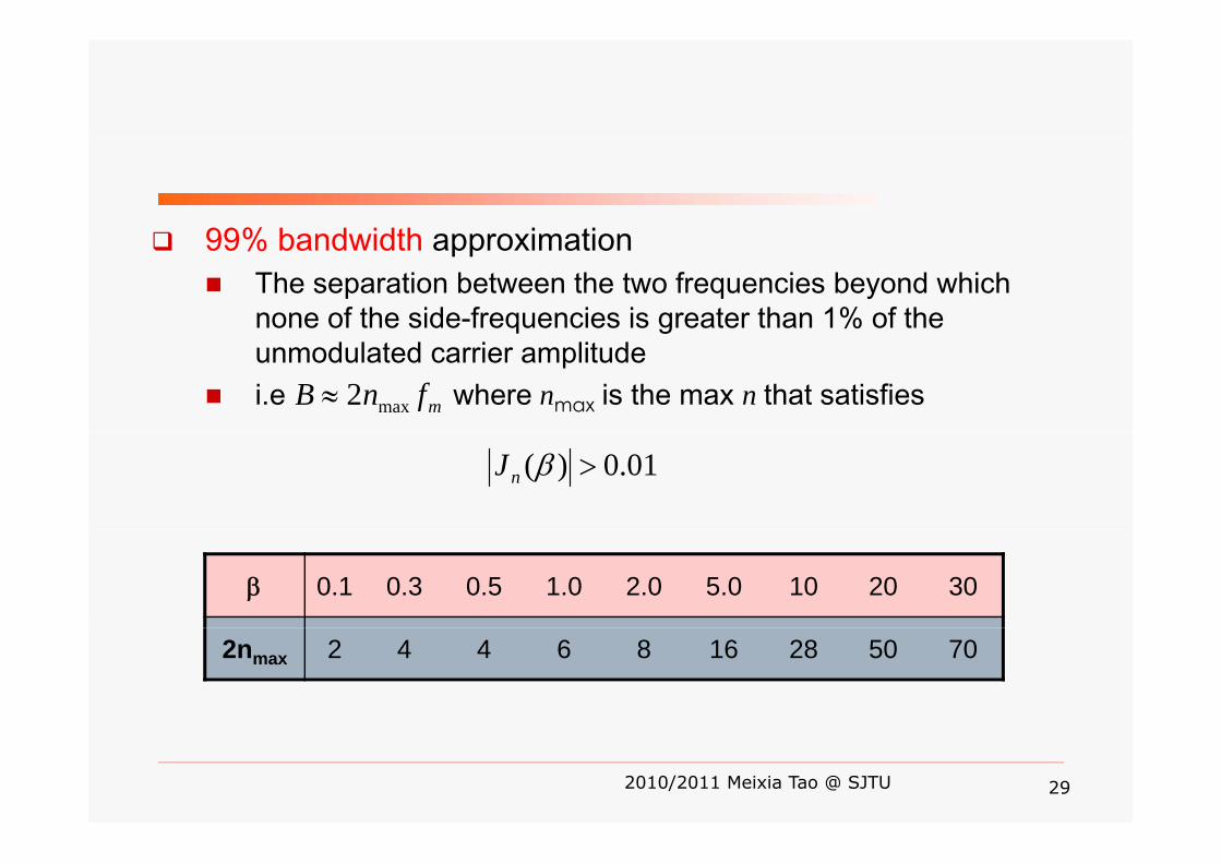
99% bandwidth approximation99% bandwidth approximationThe separation between the two frequencies beyond which none of the side-frequencies is greater than 1% of the gunmodulated carrier amplitudei.e where nmax is the max n that satisfies mfnB max2≈

01.0)( >βnJ

β 0.1 0.3 0.5 1.0 2.0 5.0 10 20 30

2nmax 2 4 4 6 8 16 28 50 70


A universal curve for evaluating the 99% bandwidth As β increases, the bandwidth occupied by the significant side-frequencies drops toward that over which the carrier frequencyfrequencies drops toward that over which the carrier frequency actually deviates, i.e. B become less affected by β

20

2


0.2 2

FM by an Arbitrary MessageFM by an Arbitrary MessageConsider an arbitrary m(t) with highest freq component WConsider an arbitrary m(t) with highest freq component W

Define deviation ratio D = Δf / W, where max ( )ff k m tΔ =

D ⇔ β and W ⇔ fm

Carson’s rule applies as

( )2 2 2 1B f W W D≈ Δ + = +

Carson’s rule somewhat underestimate the FM bandwidth requirement, while universal curve yields a somewhat conservative result

Assess FM bandwidth between the bounds given by


Carson’s rule and the universal curve

E lExampleI th A i th i l f fIn north America, the maximum value of frequency deviation Δf is fixed at 75kHz for commercial FM broadcasting by ratio. If we take the modulation frequency W = 15kHz, which is typically the maximum audio frequency of interest in FM transmission the corresponding value of the deviation ratiotransmission, the corresponding value of the deviation ratio is D = 75/15 = 5Using Carson’s rule the approximate value of theUsing Carson s rule, the approximate value of the transmission bandwidth of the FM wave is

B = 2 (75+15) = 180kHz( )Using universal curve,

B = 3 2 Δf = 3 2 x 75 = 240kHz2010/2011 Meixia Tao @ SJTU 32

B = 3.2 Δf = 3.2 x 75 = 240kHz

E iExercise( )4Assuming that , determine the

transmission bandwidth of an FM modulated signal with

( )4( ) 10sinc 10m t t=

4000k =with 4000fk =


G ti f FMGeneration of FM wavesDirect approach

Design an oscillator whose frequency changes with the input voltage => voltage controlled oscillator (VCO)input voltage => voltage-controlled oscillator (VCO)

Indirect approachFirst generate a narrowband FM signal and thenFirst generate a narrowband FM signal and then change it to a wideband signalDue to the similarity of conventional AM signals, the y g ,generation of a narrowband FM signal is straightforward.


Generation of Narrow-band FMGeneration of Narrow-band FM

Consider a narrow band FM waveConsider a narrow band FM wave

where

[ ])(2cos)( 1111 ttfAts φπ +=

∫t f = carrier frequencywhere

Gi en φ (t) <<1 ith β ≤ 0 3 e ma se

∫=t

dmkt011 )(2)( ττπφ f1 = carrier frequency

k1 = frequency sensitivity

Given φ1(t) <<1 with β ≤ 0.3, we may use[ ][ ]⎩

⎨⎧

≈≈

)()(sin1)(cos 1

ttt

φφφ

Correspondingly, we may approximate s1(t) as

[ ]⎩ ≈ )()(sin 11 tt φφ

( ) ( ) ttfAtfAt )(2i2)( φ( ) ( )( ) ( )∫−=

−=t

dmtfAktfA

ttfAtfAts

011111

111111

)(2sin22cos

)(2sin2cos)(

ττπππ

φππ


Narrow-band FW wave

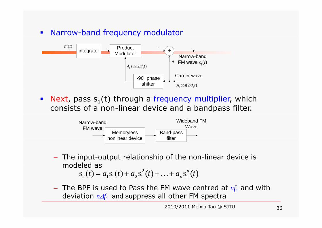
Narrow-band frequency modulator

integratorm(t) Product

Modulator +-

+Narrow-bandFM wave s (t)

q y

)2sin( 11 tfA π

-900 phaseshifter )2cos( 11 tfA π

Carrier wave

+ FM wave s1(t)

Next, pass s1(t) through a frequency multiplier, which consists of a non-linear device and a bandpass filter.

Memorylessnonlinear device

Narrow-bandFM wave

Band-passfilter

Wideband FMWave

– The input-output relationship of the non-linear device is modeled as

o ea de ce e

)()()()( 1212112 tsatsatsats n

n+++= Kmodeled as

– The BPF is used to Pass the FM wave centred at nf1 and with


1deviation nΔf1 and suppress all other FM spectra

Example: frequency multiplier with n = 2a p e eque cy u p e

Problem: Consider a square law device based frequency multiplierProblem: Consider a square-law device based frequency multiplier

with)()()( 2

12112 tsatsats +=

⎟⎞⎜⎛ ∫twith

Specify the midband freq. and bandwidth of BPF used in the freq. f f

⎟⎠⎞⎜

⎝⎛ += ∫

tdmktfAts

01111 )(22cos)( ττππ

multiplier for the resulting freq. deviation to be twice that at the input of the nonlinear deviceSolution:Solution:

⎞⎛⎞⎛

⎟⎠⎞⎜

⎝⎛ ++⎟

⎠⎞⎜

⎝⎛ += ∫∫

tt

tt

AaAa

dmktfAadmktfAats

22

01122

12011112 )(22cos)(22cos)( ττππττππ

⎟⎠⎞⎜

⎝⎛ +++⎟

⎠⎞⎜

⎝⎛ += ∫∫

ttdmktfAaAadmktfAa

0111212

01111 )(44cos22

)(22cos ττππττππ

fc=2f1


Removed by BPF with BW > 2Δf = 4Δf1

Thus connecting the narrow-band frequency modulatorThus, connecting the narrow-band frequency modulator and the frequency multiplier, we may build the wideband frequency modulator

⎞⎛q y

Message Wid b d

⎟⎠⎞⎜

⎝⎛ += ∫

tdmktfAts

01111 )(22cos)( ττππ

Integrator

Messagesignal Narrow-band

phasemodulator

WidebandFM signalFrequency

multiplier

(2 )A f tCrystal-controlled

oscillator

1cos(2 )cA f tπ

⎥⎦⎤

⎢⎣⎡ += ∫

t

fcc dmktfAts0

)(22cos)( ττππ 1

1

nkknff

f

c

==


⎥⎦⎢⎣ ∫01fnf Δ=Δ

MiMixerf f may not be the desired carrier frequency. The modulator performs an up/down conversion to shift the modulated signal to the desired center freq

1cf nf=

the modulated signal to the desired center freq. This consists of a mixer and a BPF

(t)s(t) v2(t)v1(t) Band-pass filter

)2cos( tflπ


Exercise: A typical FM transmitterExercise: A typical FM transmitter

Problem: Gi th i lifi d bl k di f t i l FMProblem: Given the simplified block diagram of a typical FM transmitter used to transmit audio signals containing frequencies in the range 100Hz to 15kHz. Desired FM wave: fc = 100MHz, Δf = 75kHz. Set β1 = 0.2 in the narrowband phase modulation to limit harmonic distortiondistortion. Specify the two-stage frequency multiplier factors n1 and n2

0.1MHz 9.5MHz


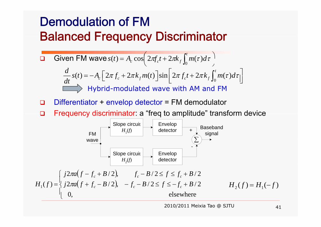
Demodulation of FMBalanced Frequency DiscriminatorBalanced Frequency Discriminator

Given FM wave ⎟⎠⎞⎜

⎝⎛ += ∫

t

fcc dmktfAts0

)(22cos)( ττππ⎠⎝ ∫fcc f

0)()(

0( ) 2 2 ( ) sin 2 2 ( )

t

c c f c fd s t A f k m t f t k m ddt

π π π π τ τ⎡ ⎤⎡ ⎤= − + +⎣ ⎦ ⎢ ⎥⎣ ⎦∫Hybrid modulated wave with AM and FM

Differentiator + envelop detector = FM demodulatorFrequency discriminator: a “freq to amplitude” transform device

Hybrid-modulated wave with AM and FM

Frequency discriminator: a freq to amplitude transform device

FMwave

Basebandsignal

Envelopdetector

Slope circuitH1(f)

∑+

wave

Slope circuitH2(f)

Envelopdetector

∑-

( )( )

⎪

⎪⎨

⎧+−≤≤−−−++≤≤−+−

= 2/2/,2/22/2/ ,2/2

)(1 BffBfBffajBffBfBffaj

fH ccc

ccc

ππ

)()( 12 fHfH −=


⎪⎩ elsewhere ,0

Circuit diagram and frequency response


Thi kThink …Compared with amplitude modulation, angle modulation requires a higher implementation complexity and a higher bandwidth occupancycomplexity and a higher bandwidth occupancy.

What is the usefulness of angle modulation systems?What is the usefulness of angle modulation systems?


Application: FM Radio broadcastingApplication: FM Radio broadcastingAs with standard AM radio most FM radio receivers areAs with standard AM radio, most FM radio receivers are of super-heterodyne type

Typical freq parameters

Limiter

Typical freq parameters– RF carrier range = 88~108

MHzLimiter

discriminator

– Midband of IF = 10.7MHz– IF bandwidth = 200kHz

Baseband low-pass filter

l d k

– Peak freq. deviation = 75KHz

Audio amplifier with de-emphasis

loudspeaker


FM Radio Stereo M ltiple ingFM Radio Stereo MultiplexingStereo multiplexing is a form of FDM ∑

+ml(t)Stereo multiplexing is a form of FDM designed to transmit two separate signals via the same carrier. Widely used in FM broadcasting to

∑

∑ ∑

++

-

mr(t)+

+ m(t)

Widely used in FM broadcasting to send two different elements of a program (e.g. vocalist and accompanist in an orchestra) so as to

Frequencydoubler

K

accompanist in an orchestra) so as to give a spatial dimension to its perception by a listener at the receiving end

)2cos( tf cπ

[ ][ ]

)()()( tmtmtm rl +=receiving end [ ]

)2cos()4cos()()(

tfKtftmtm

c

crl

ππ

+−+

The sum signal is left unprocessed in its baseband formTh diff i l d 38 kH The difference signal and a 38-kHz subcarrier produce a DSBSC waveThe 19-kHz pilot is included as a

f f h t d t ti

fc = 19kHz

2010/2011 Meixia Tao @ SJTU10/4/2004 45

reference for coherent detection

FM Stereo ReceiverFM-Stereo Receiver

Baseband LPF

m(t)

∑+

++

2ml(t)ml(t)+mr(t)

To two loudspeakersBPF centered at 2fc=38kHz

Frequency

m(t)∑

+

- 2mr(t)

Baseband LPF

ml(t)-mr(t)

Narrow-band filter tuned to

f 19kH

Frequency doubler

fc=19kHz

2010/2011 Meixia Tao @ SJTU10/4/2004 46

ff f3.4 Effect of Noise on Angle Modulation

Block diagram of an angle demodulator

( ) ( )s t n t+( ) ( ) ( )r t s t n t= + ( )y t S

N⎛ ⎞⎜ ⎟⎝ ⎠BPF

BW=Bc Demod LPFBW=W

( ) ( )ws t n t+ oN⎝ ⎠

Input to the demodulator is( ) ( )s t n t+

[ ]cos ( ) ( )cos ( )sinA t t n t t n t tω φ ω ω= + + −

( )r t =

[ ]cos ( ) ( )cos ( )sinc c c c s cA t t n t t n t tω φ ω ω= + + −

( )cos( ( ))n c nR t w t tθ= +


( ) ( ( ))n c n

Assume that the signal is much larger than the noise( )( ) ( )cos ( ) ( )c n nr t A R t t tθ φ≈ + − ⋅⎡ ⎤⎣ ⎦

( )( )

1 ( )sin ( ) ( )cos ( )

( )cos ( ) ( )n n

cc n n

R t t tw t t tg

A R t t tθ φ

φθ φ

−⎛ ⎞−+ +⎜ ⎟⎜ ⎟+ −⎝ ⎠

( )nR t( )c n n⎝ ⎠

The phase term can be further approximated as

( )sn t( )

etθ ( ) ( )

nt

tθ

φ−

( )yR

tcA( )( )( ) ( ) sin ( ) ( )n

r nc

R tt t t tA

θ φ θ φ= + −

pp

( )n t

( )nR t( )tφ ( )y tθ ( )n tθ


( )cn t2 2 ( )cA E n t⎡ ⎤⎣ ⎦

Th f h f h d d l iTherefore, the output of the demodulator is

( )( )( ) ( ) ( ) sin ( ) ( )nr f n

R td dy t t k m t t tθ θ φ= = + −( )( ) ( ) ( ) ( ) ( )2 2

( ) ( )2

r f nc

f n

ydt dt A

dk m t Y tdt

φπ π

= +2f ndtπ

Desired signal Noise

The noise component is inversely proportional to the signal amplitude Ac. (This is not the case for AM system)

( ) 1R t ( ) [ ]( ) 1( ) sin ( ) ( ) ( )cos ( ) ( )sin ( )nn n s c

c c

R tY t t t n t t n t tA A

θ φ φ φ= − = −

[ ]1 ( )cos ( )sinn t n tφ φ= − (Since is slowly varying)( )tφ


[ ]( )cos ( )sins cc

n t n tA

φ φ= (Since is slowly varying)( )tφ

1 dThe power spectral density of is 1 ( )2 n

d Y tdtπ

2 22 24 cos sinfπ φ φ⎡ ⎤⎛ ⎞ ⎛ ⎞⎢ ⎥2

2

2

4 cos sin( ) ( ) ( )4 n s cY n n

c c

f S f f S f S fA A

f

π φ φπ

⎡ ⎤⎛ ⎞ ⎛ ⎞⎢ ⎥= +⎜ ⎟ ⎜ ⎟⎢ ⎥⎝ ⎠ ⎝ ⎠⎣ ⎦

⎧202

2

2( )

0 otherwisec

Cn c

c

f N f Bf S f AA

⎧≤⎪= = ⎨

⎪⎩⎩

( )nfS f( )noS f

At the output of LPF, the noise is limited to the freqnoise is limited to the freq. range [-W, W]

2010/2011 Meixia Tao @ SJTU 50xf− xf2TB− 2TB fW-W

Now we can determine the output SNR in FMFirst, the output signal power is

The output noise power is2

os f mP k P=

320 0

2 2

23o

W

n Wc c

N N WP f dfA A−

= =∫Then, the output SNR is

0

2 23s f c mP k A PS⎛ ⎞

⎜ ⎟23 f mP Sβ ⎛ ⎞

⎜ ⎟0

202

o

f m

o nN P W N W= =⎜ ⎟

⎝ ⎠ ( )2max ( )

f

bNm t= ⎜ ⎟

⎝ ⎠


Ob tiObservationsIncreasing the modulation index increases the output SNR, in contrast to AMI i th b d idth i th t t SNR

β

Increasing the bandwidth increases the output SNR.Therefore, angle modulation provides a way to trade off bandwidth for transmitted poweroff bandwidth for transmitted powerIncreasing the transmitted power increases output SNR in both FM and AM systems, but the y ,mechanisms are totally different (explain!)Increasing up to a certain value improves the βg p pperformance, but cannot continue indefinitely due to the threshold effect

β


Th h ld Eff tThreshold EffectThere exists a specific SNR at the input of the demodulator below which the signal is not distinguishable from the noisedistinguishable from the noise

FMS FM

DSB

0

0

NS

DSB

i

i

NS


0 a

C i f A l M d l tiComparison of Analog-ModulationBandwidth efficiencyBandwidth efficiency

SSB is the most bandwidth efficient, but cannot effectively transmit DCVSB is a good compromisePM/FM are the least favorable systems

Power efficiencyPower efficiencyFM provides high noise immunityConventional AM is the least power efficient

Ease of implementation (transmitter and receiver)The simplest receiver structure is conventional AMFM receivers are also easy to implementFM receivers are also easy to implementDSB-SC and SSB-SC requires coherent detector and hence is much more complicated.


A li tiApplicationsSSB-SC:

Voice transmission over microwave and satellite linksVSB SCVSB-SC

Widely used in TV broadcastingFMFM

High-fidelity radio broadcastingC ti l AMConventional AM

AM radio broadcastingDSB SCDSB-SC

Hardly used in analog signal transmission!


Date post:	13-Jan-2017
Category:	Documents
Upload:	phamkien
View:	217 times
Download:	1 times

Pi i l f C i i Principles of Communications

Documents