Additional information is available at the end of the chapter
http://dx.doi.org/10.5772/48497
1. Introduction Many industrial applications have digital closed loop control systems and the main algorithm used at these applications is the Proportional Integral Derivative structure (PID). This chapter presents some useful MATLAB commands that might be used as an instrument to analyze the closed loop and also to help the control system design. The first part presents the general standard structure of this controller, whereas MATLAB/SIMULINK programs are used to illustrate some design aspects. Script codes are used to describe the dynamic systems through the Laplace Transform and time response analysis of the system with time delays. Block diagram descriptions employed to represent the distillation process are used to analyses the Proportional Integral controller (PI) applied to the system. Performance analysis is conducted to implement an exhaustive searching algorithm applied in tuning PI parameters. At the second part a Smith Predictor structure is designed and presented to enhance the system performance. Some common feedback structures are presented and the classical literature will be referenced to present the main topics.
Along the chapter the tuning algorithms and the system analyses tools are presented through a specific application. This example is related to the tuning of PI control system applied to the temperature and pressure control in a distillation process designed to obtain the anhydrous ethanol and the hydrated ethanol from the sugarcane fermentation and distillation.
2. PID structures In the literature, several works has describing the PID structure (Ǻström & Hägglund, 1995), (Ang, 2008), (Mansour, 2011) and (Alfaro, 2005). According to the authors the three term form is the standard PID structure of this controller. The structure is also known as parallel form and is represented by:
1 1( ) 1p I D p DI
G s K K K s K T ss T s
(1)
MATLAB – A Fundamental Tool for Scientific Computing and Engineering Applications – Volume 1
4
Where:
Kp : proportional gain; KI : integral gain; KD : derivative gain; TI : integral time constant and TD : derivative time constant.
In MATLAB, the script code of parallel form may be represented by:
s = tf('s'); % PID Parallel form Kp=10; Td=0.1; Ti=0.1; G=Kp*(1+(1/(Ti*s))+Td*s);
The control parameters are:
- The proportional term: providing an overall control action proportional to the error signal through the constant gain factor.
- The integral term: the action is to reduce steady-state errors through low-frequency compensation by an integrator.
- The derivative term: improves transient response through high-frequency compensation by a differentiator.
The very same system may be designed at SIMULINK Toolbox, represented in figure 1.
Figure 1. Simulink PID Control
To minimize the gain at high frequencies, the derivative term is usually modified to:
PID Control Design
5
1( ) 11
Dp
I D
T sG s K
T s T s
(2)
Where α is a positive parameter adjusted between 0.01 and 1. This formulation is also used to obtain a causal relationship between the input and the output of the controller. Another usual structure employed at the PID controller is presented in figure 2.
Figure 2. PID Controller with derivative term at the feedback branch.
According to this configuration, the derivative term is inserted out of the direct branch. The structure is carried to minimize the effect of set-point changes at the output of the control algorithm. By using this configuration only variations at the output signal of the plant will be added with the integral and proportional actions.
2.1. Tuning methods
Several tuning methods are described in (Ǻström & Hägglund, 1995) and in (Ang, 2007). The tuning methods are employed to obtain the stability of the closed-loop system and to meet given objectives associated with the following characteristics:
stability robustness; set-point following and tracking performance at transient response, including rise-time,
overshoot, and settling time; regulation performance at steady-state, including load disturbance rejection; robustness against plant modelling uncertainty; noise attenuation and robustness against environmental uncertainty.
In (Ang, 2007), the PID controllers tuning methods are classified and grouped according to their nature and usage. The groups that describe each tuning method are:
Analytical methods—at these methods the PID parameters are calculated through the use of analytical or algebraic relations based in a plant model representation and in some design specification.
MATLAB – A Fundamental Tool for Scientific Computing and Engineering Applications – Volume 1
6
Heuristic methods—These methods are evolved from practical experience in manual tuning and are coded trough the use of artificial intelligence techniques, like expert systems, fuzzy logic and neural networks.
Frequency response methods—the frequency response characteristics of the controlled process is used to tune the PID controller. Frequently these are offline and academic methods, where the main concern of design is stability robustness since plant transfer function have unstructured uncertainty.
Optimization methods—these methods utilize an offline numerical optimization method for a single composite objective or use computerised heuristics or, yet, an evolutionary algorithm for multiple design objectives. According to the characteristics of the problem, an exhaustive search for the best solution may be applied. Some kind of enhanced searching method may be used also. These are often time-domain methods and mostly applied offline. This is the tuning method used at the development of this work.
Adaptive tuning methods—these methods are based in automated online tuning, where the parameters are adjusted in real-time through one or a combination of the previous methods. System identification may be used to obtain the process dynamics over the use of the input-output data analysis and real time modelling.
2.2. Measures of controlled system performance
A set of performance indicators may be used as a design tool aimed to evaluate tuning methods results. These performance indicators are listed from (3) to (6) equations.
Integral Squared Error (ISE)
20
( )T
ISEJ e t dt (3)
Integral Absolute Error (IAE)
0
( )T
IAEJ e t dt (4)
Integral Time-weighted Absolute Error (ITAE)
0
( )T
ITAEJ t e t dt (5)
Integral Time-weighted Squared Error (ITSE)
2
0
( )T
ITSEJ t e t dt (6)
PID Control Design
7
These indicators can help the design engineer to decide about the best adjustment for the PID control parameters. In (Cao, 2008) it is presented some MATLAB codes to obtain these indicators.
3. Distillation column dynamics
In Brazil approximately 50% of vehicle fleet is composed of flex vehicles, resulting in 30 million of vehicles. This kind of vehicle uses fossil fuel and/or ethanol. The ignition system is adjusted automatically depending of the proportion of each fuel kind. To attend the national ethanol demand there are several ethanol distillation facilities across the country. In each of these facilities the fermented sugarcane is distilled, obtaining two products: the anhydrous ethanol and the hydrated ethanol.
The hydrated ethanol is obtained from link between the second and the third column. The anhydrous ethanol is obtained at the base of the third column, see Figure 3. The production process is composed of a series of columns where two variables are controlled to generate the hydrated ethanol and the anhydrous ethanol at the standardized specification: the pressure at the column A and the temperature at the distillation tray A20 (Santos et al., 2010). The hydrated ethanol has to have a concentration of 92,6 oINPM (oINPM is a measurement of the weight of pure ethanol fuel in 100g of ethanol fuel – water mixture). So as near the concentration is about this value, the best will be the quality of the hydrated ethanol and the anhydrous ethanol.
Figure 3. Distillation process to produce anhydrous ethanol and the hydrated ethanol.
MATLAB – A Fundamental Tool for Scientific Computing and Engineering Applications – Volume 1
8
These variables depend respectively on the steam flow at the basis of the column A and on the flow of fermented mash applied at the column A. The minimization of the variability of the alcoholic content according the brazilian standard NBR 5992-80 is the main design objective of the control system.
The distillation process is characterized by a high coupling through the system variables and by a non-linear relationship between them. According (Santos, 2010) the models that represent the relationship between the main process variables is FOTD (First Order with Time Delay).
( )1
sKeG ss
(7)
In this work the modeling procedure was developed and the following equation was obtained from the relationship of the pressure variation at the A column and the steam flow valve actuation:
1 0
2 1
(0,36 0,44).110%55 85,91
0,26% / %323
PVKMV
K bar opennigt t st t s
(8)
Where MP is the Manipulated Variable e PV is the Process Variable.
So, the FODT representation is:
30,26( )
23 1
seG ss
(9)
The same modeling procedure was developed to obtain the relationship among the variation of the temperature at the distillation tray A20 and the variation of the flow of fermented mash applied at the column A:
1 0
2 1
(97,8 95,8) .110%150´23% 33%
´ 0,133% / %
´ 85´ 174
oopennig
PVKMV
K C
t t st t s
(10)
So, the FODT representation is:
850,133( )
174 1
seG ss
(11)
PID Control Design
9
3.1. Tuning methods
The above systems were described in (Santos, 2010) and at that work there also were described and applied four tuning methods of the PI control: Ziegler-Nichols (First Method), CHR, Cohen-Coon and IMC (Internal Model Control).
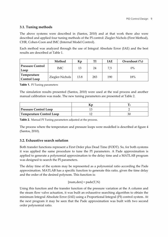
Each method was analyzed through the use of Integral Absolute Error (IAE) and the best results are described at Table 1.
Method Kp TI IAE Overshoot (%) Pressure Control Loop IMC 13 24 7,5 0%
Temperature Control Loop Ziegler-Nichols 13.8 283 190 18%
Table 1. PI Tuning parameters
The simulation results presented (Santos, 2010) were used at the real process and another manual calibration was made. The new tuning parameters are presented at Table 2.
Kp TI Pressure Control Loop 13 2 Temperature Control Loop 12 30
Table 2. Manual PI Tuning parameters adjusted at the process.
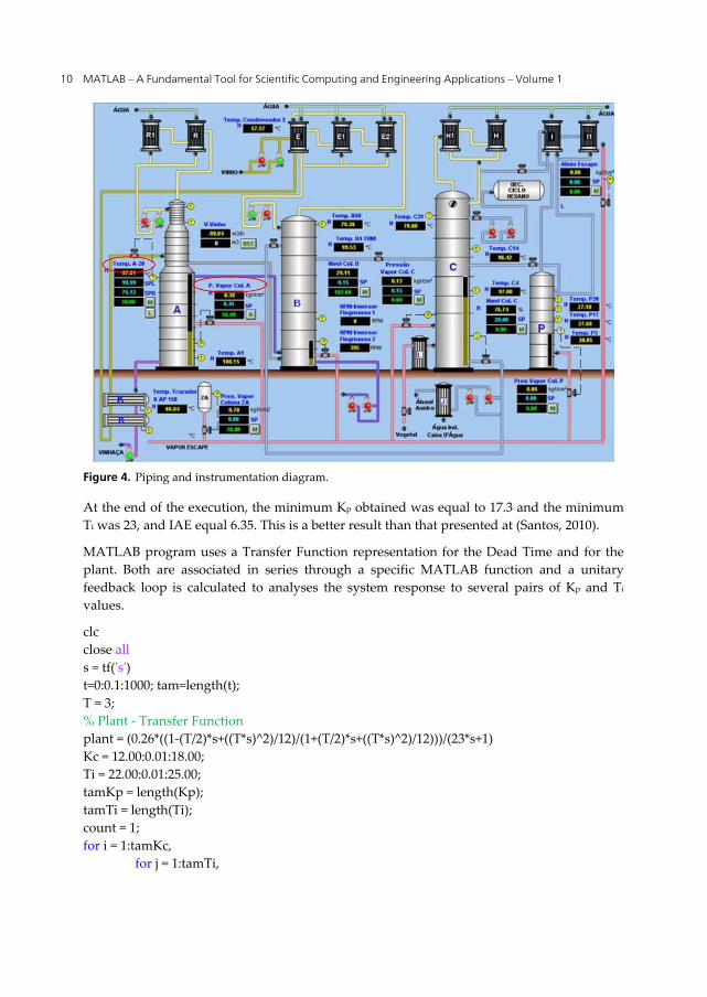
The process where the temperature and pressure loops were modelled is described at figure 4 (Santos, 2010).
3.2. Exhaustive search solution
Both transfer functions represent a First Order plus Dead Time (FODT). So, for both systems it was applied the same procedure to tune the PI parameters. A Pade approximation is applied to generate a polynomial approximation to the delay time and a MATLAB program was designed to search the PI parameters.
The delay time of the system may be represented as a polynomial ratio according the Pade approximation. MATLAB has a specific function to generate this ratio, given the time delay and the order of the desired polynom. This function is:
[num,den] = pade(T,N)
Using this function and the transfer function of the pressure variation at the A column and the steam flow valve actuation, it was built an exhaustive searching algorithm to obtain the minimum Integral Absolute Error (IAE) using a Proportional Integral (PI) control system. At the next program it may be seen that the Pade approximation was built with two second order polynomial ratio.
MATLAB – A Fundamental Tool for Scientific Computing and Engineering Applications – Volume 1
10
Figure 4. Piping and instrumentation diagram.
At the end of the execution, the minimum Kp obtained was equal to 17.3 and the minimum Ti was 23, and IAE equal 6.35. This is a better result than that presented at (Santos, 2010).
MATLAB program uses a Transfer Function representation for the Dead Time and for the plant. Both are associated in series through a specific MATLAB function and a unitary feedback loop is calculated to analyses the system response to several pairs of Kp and Ti
values.
clc close all s = tf('s') t=0:0.1:1000; tam=length(t); T = 3; % Plant - Transfer Function plant = (0.26*((1-(T/2)*s+((T*s)^2)/12)/(1+(T/2)*s+((T*s)^2)/12)))/(23*s+1) Kc = 12.00:0.01:18.00; Ti = 22.00:0.01:25.00; tamKp = length(Kp); tamTi = length(Ti); count = 1; for i = 1:tamKc, for j = 1:tamTi,
PID Control Design
11
PI = Kp(i)*(1+1/(Ti(j)*s)); H=series(PI,plant); L=feedback(H,1); [output, t] = step(L,t); MP = Calcul_MP(output); IAE = IAE_U_Step(output,0.1); result(count,1) = Kp(i); result(count,2) = Ti(j); result(count,3) = MP; result(count,4) = IAE; count = count+1; end count end % Search for minimum Kc and minimum Ti tam = length(result) minimumIAE = 1000 for i=1:tam(1), if minimumIAE > result(i,4) minimumIAE = result(i,4); minimumKp = result(i,1); minimumTi = result(i,2); end end minimumIAE minimumKp minimumTi
At the program listed above, two other functions were developed: Calcul_Mp and IAE_U_Step.
These functions are listed below:
function [MP] = CalculMP(output) tam = length(output); MP = (max(output)-output(tam))/output(tam)*100; end
At the function CalculMP the output length is obtained to take the last value of the output variable to the step response. It is used to calculate the overshoot of the system.
At the next function the Integral Absolute Error (IAE) is numerically obtained using the output generated at the main mathscript code.
function [IAE_Value] = IAE_U_Step(output,int_T) Tam = length(output); IAE_Value = 0;
MATLAB – A Fundamental Tool for Scientific Computing and Engineering Applications – Volume 1
12
for i=1:Tam, if output(i) < 1 IAE_Value = IAE_Value + (1-output(i))*int_T; else IAE_Value = IAE_Value + (1-output(i))*(-1)*int_T ; end end end
The closed loop system model with a PI control was built at SIMULINK as represented at figure 5.
Figure 5. Closed loop Pressure Control with Pade approximation.
Applying a step function from 51 bar to 85 bar at the input of the system presented at figure 5, the output is presented at figure 6 for the tuning parameters obtained at the exhaustive search algorithm.
0 5 10 15 20 25 3045
50
55
60
65
70
75
80
85
90
Time(s)
Pre
ssur
e
Pressure Response
Figure 6. Step response of the closed loop pressure control system.
PID Control Design
13
The step response presented at Figure 6 represents a fast response with low overshoot than that presented at (Santos, 2010). It is possible to verify the delay time at the output signal.
The same procedure was used to design the control algorithm to the temperature loop and best results were obtained when compared with those presented at (Santos, 2010). In both closed loops the exhaustive search for the best response was executed near the initial solution obtained through the experimental tuning procedure.
4. Smith Predictor design
A design tool very useful to control engineers when it is necessary to design a control system with delay at time response is the Smith Predictor (Ogata, 2009). At the distillation plant both SISO systems are represented by transfer functions with time delays. At this item it is done some considerations about the use of this technique to generate better results for the time response of the system. The control structure of the Smith Predictor is presented at figure 7.
Figure 7. Smith Predictor Structure.
In the system presented at figure 7, H(s) represents the pure delay time and F(s) represents the plant transfer function without delay. Analysing as separated parts, it is proposed a controller with input E(s) and output U(s) that has the delay time transfer function H(s) and F(s) modelled in its structure. It is possible to analyse the system proposed and verify that its transfer function C(s)/R(s) is equal to the transfer function of the system presented at figure 8.
Figure 8. Equivalent system.
MATLAB – A Fundamental Tool for Scientific Computing and Engineering Applications – Volume 1
14
At figure 8 it is possible to verify that G(s) may be designed considering the transfer function F(s) without the time-delay. The transfer function of the complete system has the design specification plus the dead time present at the original plant.
4.1. MATLAB code implementing Smith Predictor
To analyse the system performance with a Smith Predictor structure it was developed a MATLAB code and a SIMULINK model. The mathscript code is presented below, with a Pade approximation to represent the time delay. The polynomial ratio used at the next code represents a delay of 3 seconds with the ratio of two second order polynomials. The block association was developed through the use of the association commands series and feedback.
Representing the Smith Predictor in a MATLAB code:
% Smith Predictor clc clear all close all s=tf('s') % Delay with Pade aproximation [num_d,den_d]=pade(3,2) % PI Control System Kp=2; Ti=15; G=Kp*(1+(1/(Ti*s))); H=tf(num_d,den_d) Gc=feedback(G,series((1-H),(0.26/(23*s+1)))) CL=feedback(series(Gc,series(tf(num_d,den_d),0.26/(23*s+1))),1) figure(1) step(CL,200) grid
It is possible to see that the association Gc represents the control algorithm, where G is the Proportional Integral controller designed to the plant without delay. The system designed with SIMULINK model is presented at figure 9.
At the next figure the step response obtained at the end of the program. It is possible to see that the stationary error is equal to zero and that the control parameters could be adjusted to obtain a small overshoot.
PID Control Design
15
TransportDelay
0.26
23s+1
0.26
23s+1
Step
Scope
Kp
2
Integrator
1s
1/Ti
1/15
Figure 9. Smith Predictor in SIMULINK model.
0 20 40 60 80 100 120 140 160 180 200-0.2
0
0.2
0.4
0.6
0.8
1
1.2Step Response
Time (sec)
Am
plitu
de
Figure 10. Closed loop system response.
0 5 10 15 20 25 30 35 40 45 500
0.5
1
1.5
2
2.5
3
3.5
4Controller Output
time(s) Figure 11. Controller output.
MATLAB – A Fundamental Tool for Scientific Computing and Engineering Applications – Volume 1
16
The output of the controller must be verified after the control system design to avoid the saturation of the actuators.
4.2. Digital control design
The control algorithm designed through the Smith Predictor may be described in a digital form, using the Z-Transform representation. The MATLAB script code below represents this transfer function.
% Digital Smith Predictor clc clear all close all s=tf('s') Kp=2; Ti=15; G=Kp*(1+(1/(Ti*s))); T=0.1; Gz=c2d(G,T,'tustin') n=3/T; z=tf('z',0.1) Hz=c2d(0.26/(26*s+1),T,'tustin') Gcz=feedback(Gz,series(Hz,1-z^(-n))
The G transfer function represents the Proportional Integral algorithm and Gz is its discrete form using the Bilinear (Tustin) approximation. The sample time was adjusted in 0.1 s, since the dimension of time delay is about 30 times greater than this value. The time delay verified at the system may be easily modelled measuring how many samples the system measure along the total time delay. This measurement is represented at n=3/T.
The digital controller designed is represented by:
...0.001 ( 30) 0.000006 ( 31) 0.00099 ( 32)u k e k e k e k u k u k
u k u k u k
(12)
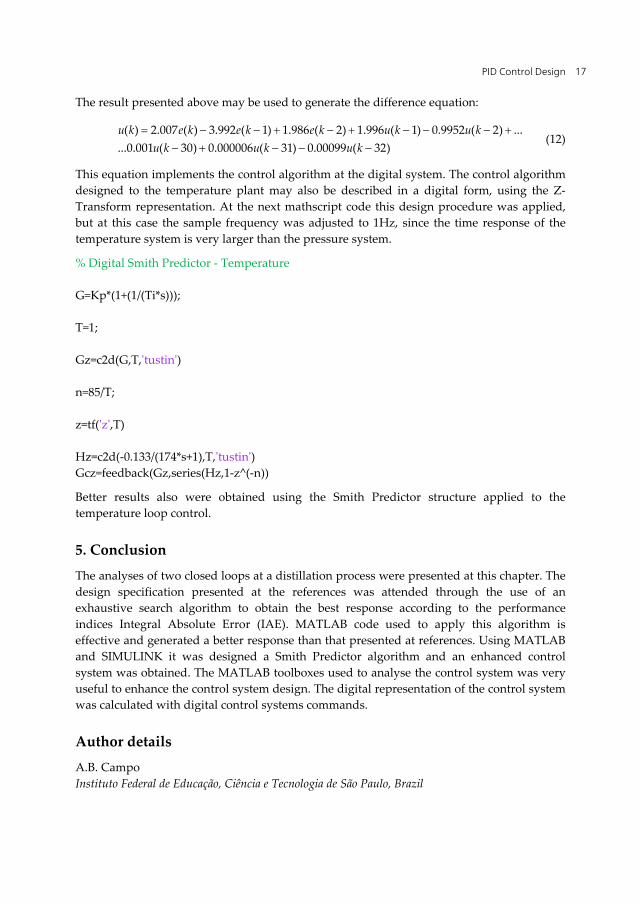
This equation implements the control algorithm at the digital system. The control algorithm designed to the temperature plant may also be described in a digital form, using the Z-Transform representation. At the next mathscript code this design procedure was applied, but at this case the sample frequency was adjusted to 1Hz, since the time response of the temperature system is very larger than the pressure system.
% Digital Smith Predictor - Temperature G=Kp*(1+(1/(Ti*s))); T=1; Gz=c2d(G,T,'tustin') n=85/T; z=tf('z',T) Hz=c2d(-0.133/(174*s+1),T,'tustin') Gcz=feedback(Gz,series(Hz,1-z^(-n))
Better results also were obtained using the Smith Predictor structure applied to the temperature loop control.
5. Conclusion
The analyses of two closed loops at a distillation process were presented at this chapter. The design specification presented at the references was attended through the use of an exhaustive search algorithm to obtain the best response according to the performance indices Integral Absolute Error (IAE). MATLAB code used to apply this algorithm is effective and generated a better response than that presented at references. Using MATLAB and SIMULINK it was designed a Smith Predictor algorithm and an enhanced control system was obtained. The MATLAB toolboxes used to analyse the control system was very useful to enhance the control system design. The digital representation of the control system was calculated with digital control systems commands.
Author details
A.B. Campo Instituto Federal de Educação, Ciência e Tecnologia de São Paulo, Brazil
MATLAB – A Fundamental Tool for Scientific Computing and Engineering Applications – Volume 1
18
Acknowledgement
The author would like to thanks Instituto Federal de Educação, Ciência e Tecnologia de São Paulo for the MATLAB license and hardware resources used at the development of this work.
6. References
Alfaro, V. M., Vilanova, R. Arrieta O. Two-Degree-of-Freedom PI/PID Tuning Approach for smooth Control on Cascade Control Systems, Proceedings of the 47th IEEE Conference on Decision and Control Cancun, Mexico, Dec. 9-11, 2008.
Ang, K.H., Chong G. LI, Yun PID Control System Analysis, Design, and Technology, In: IEEE Transactions on Control Systems Technology, vol. 13, no. 4, july, 2005.
Ǻström, K.J. , Hägglund, T. (1995) PID controllers Setting the standard for automation 2nd Edition, 343 p., International Society for Measurement and Control.
Ǻström, K. J. , Hägglund, T. (1995) PID Controllers: Theory, Design, and Tuning, 2nd Edition ISBN 978-1-55617-516-9.
Cao, Yao. (January 2008). Learning PID Tuning III: Performance Index Optimization, In: MATLAB CENTRAL File Exchange, 08.04.2012, Available from
Mannini, P. ; Mello, V.F.; Santos, D.S.; Araújo, G.C.; Campo, A.B (2012) Projeto de controle PID em uma coluna de destilação de álcool, Revista Sinergia (submitted).
Mansour,T. (2011) PID Control, Implementation and Tuning, 238 p., InTech, ISBN 978-953-307-166-4, Rijeka, Croatia.
Ogata, K. (2009) Modern Control Engineering, 912p., 5nd. Edition, Prentice Hall ISBN-13: 978-0136156734,
Seborg, D.E.; Edgar, T.F., Mellichamp, D.A. Process Dynamics and Control, John Wiley & Sons, Singapore, 717p., 1989.
Santos, J.C. dos S.; Santos, R.P. dos; Salles, J.L.F. Redução da Variabilidade do Teor Alcoólico na Indústria Sucroalcooleira, ISA Show, Brazil, 2010.
Yurkevich, V. D. (2011) Advances in PID Control, InTech, ISBN 978-953-307-267-8, Rijeka, Croatia.