International Journal of Systems Science, 2013http://dx.doi.org/10.1080/00207721.2013.775385

PID position domain control for contour tracking

P.R. Ouyang∗, V. Pano and T. Dam

Department of Aerospace Engineering, Ryerson University, Toronto, Canada

(Received 6 January 2012; final version received 2 February 2013)

Contour error reduction for modern machining processes is an important concern in multi-axis contour tracking applicationsin order to ensure the quality of final products. Many control methods were developed in time domain to deal with contourtracking problems, and a proportional–derivative (PD) position domain control (PDC) was also proposed by the authors. It iswell known that proportional–integral–differential (PID) control is the most popular control in applications of control theory.In this paper, a PID PDC is proposed for reducing contour tracking errors and improving contour tracking performances.To determine proper control gains, system stability analysis is conducted for the proposed PDC. Several experiments areconducted to evaluate the performance of the developed approach and are compared with the PID time domain control(TDC) and the cross-coupled control. Different control gains are used in the simulations to explore the robustness of PIDPDC. Comparison results demonstrate the effectiveness and good contour performances of PID PDC for contour trackingapplications.

Keywords: position domain; PID control; contour tracking; contour error; stability

1. Introduction

In manufacturing processes, one of the most important is-sues is the reduction of machining errors to ensure thequality of final products. To achieve this goal, a good con-trol system is required in a machining system. Despite thedevelopment of various advanced control algorithms in in-dustry and academia over past a few decades, it is wellknown that proportional–integral–differential (PID) con-trol (Radke and Isermann 1987; Mills and Goldenbery1988; Qu and Dorsey 1991; Rocco 1996; Visioli and Leg-nani 2002; Astrom and Hagglund 2006; Jin, Yang, andChang 2013) is the most popular one in applications ofcontrol theory. Due to its simple structure, easy implemen-tation and robust operation, PID control is widely used forthe following applications: process control, robot manip-ulations, motor drives, automotive control, flight control,instrumentation operations, etc. Most industrial robot ma-nipulators are equipped with PID controllers that do not re-quire information about the robot dynamics in their controllaws. A linear and decoupled PID control with appropri-ate control gains can achieve the desired position withoutsteady-state error. That is the main reason for the wideapplications of PID control. It is thought that PID con-trol is the best solution from an industrial point of view(Khalil 2002). Many studies have been conducted for sta-bility analysis of PID control using different approaches(Qu and Dorsey 1991; Mills and Goldenbery 1988;Rocco 1996).

∗Corresponding author. Email: pouyang@ryerson.ca

There are two different control tasks in applications ofrobot manipulators: one is set-point (position) control thatdoes not specify the path of the end-effector, and the otheris trajectory tracking control that requires a robot manip-ulator following a specifically defined path. According tothe controlled target, robot control can be classified into twodifferent categories: one is in the joint level, and the other isin the end-effect or task space level. For the purpose of con-trol, it should be noted that the task space control should bemapped into the joint level control of the actuators throughinverse kinematic analysis.

A contour error is defined as the error between thedesired contour and the real contour in an orthogonal di-rection. The contour error is an important index to measurethe quality of a machined product or the contour track-ing performance. In a conventional approach, for example,the decoupled PID control, the contour error is controlledand improved by a tracking controller for each individ-ual axis. A common method to improve the contour accu-racy is to achieve high tracking accuracy of each individualaxis. Many efforts have been made to improve the trackingperformance through developing many advanced controlsystems, such as adaptive control (Radke and Isermann1987), robust control (Jin et al. 2013), sliding mode control(Zhao and Zou 2012), fuzzy logic control (Tzafestas andPapanikolopoulos 1990), neural network control (Miller,Hewes, Glanz, and Kraft 1990), iterative learning control(Bouakrif, Boukhetala, and Boudjea 2013), etc.

C© 2013 Taylor & Francis

Dow

nloa

ded

by [

Rye

rson

Uni

vers

ity]

at 1

2:36

22

Mar

ch 2

013

2 P.R. Ouyang et al.

It should be noted that a good tracking performancefor each individual axis does not guarantee the reductionof contour errors for a multi-axis motion system, as poorsynchronisations of relevant motion axes result in dimin-ished contour accuracy of the contour tracking (Koren 1980;Fang and Chen 2002; Barton and Alleyne 2008; Hu, Yao,and Wang 2009). To solve this problem, a so-called cross-coupled control (CCC) was proposed by Koren (1980) andextensively discussed in Fang and Chen (2002), Barton andAlleyne (2008) and Hu et al. 2009) for further improve-ments. Actually, the majority of CCC is a combinationof proportional–derivative (PD)/PID control for individualaxis and a coupled error feedback control for multiple axes.

In our previous work (Ouyang, Dam, Huang, and Zhang2012), a PD-type contour tracking control law established inposition domain was proposed, focusing on contour track-ing performance improvement. In order to further improvethe contour accuracy, a PID contour tracking control inposition domain is developed in this paper. The stabilityanalysis is conducted using the Lyapunov method, and theprinciple for selecting control gains in position domain isprovided based on the stability analysis. After that, somecomplex contour tracking problems are examined and com-pared with the traditional PID control and CCC in time do-main. Simulation results demonstrate the effectiveness andhigh contour performances of the proposed PID positiondomain control (PDC).

2. PID PDC and contour error

2.1. System description and dynamic model intime domain and position domain

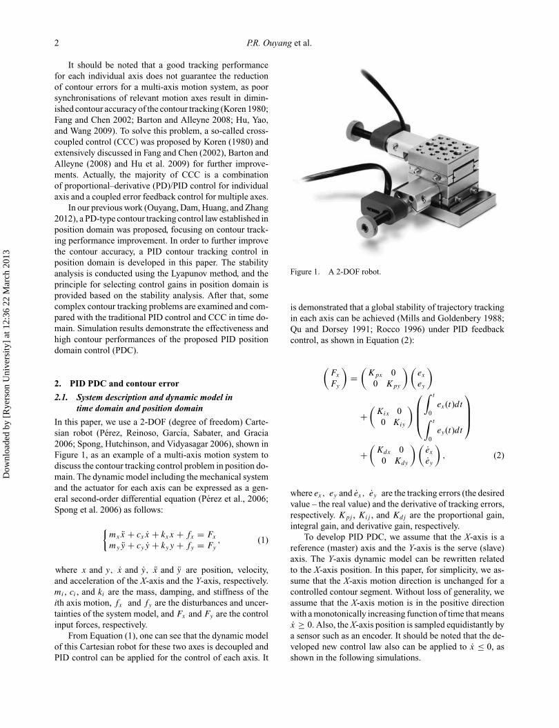
In this paper, we use a 2-DOF (degree of freedom) Carte-sian robot (Perez, Reinoso, Garcıa, Sabater, and Gracia2006; Spong, Hutchinson, and Vidyasagar 2006), shown inFigure 1, as an example of a multi-axis motion system todiscuss the contour tracking control problem in position do-main. The dynamic model including the mechanical systemand the actuator for each axis can be expressed as a gen-eral second-order differential equation (Perez et al., 2006;Spong et al. 2006) as follows:

{mxx + cxx + kxx + fx = Fx

myy + cyy + kyy + fy = Fy, (1)

where x and y, x and y, x and y are position, velocity,and acceleration of the X-axis and the Y-axis, respectively.mi , ci , and ki are the mass, damping, and stiffness of theith axis motion, fx and fy are the disturbances and uncer-tainties of the system model, and Fx and Fy are the controlinput forces, respectively.

From Equation (1), one can see that the dynamic modelof this Cartesian robot for these two axes is decoupled andPID control can be applied for the control of each axis. It

Figure 1. A 2-DOF robot.

is demonstrated that a global stability of trajectory trackingin each axis can be achieved (Mills and Goldenbery 1988;Qu and Dorsey 1991; Rocco 1996) under PID feedbackcontrol, as shown in Equation (2):

(Fx

Fy

)=

(Kpx 0

0 Kpy

)(ex

ey

)

+(

Kix 00 Kiy

) ⎛⎜⎜⎝

∫ t

0ex(t)dt∫ t

0ey(t)dt

⎞⎟⎟⎠

+(

Kdx 00 Kdy

) (ex

ey

), (2)

where ex, ey and ex , ey are the tracking errors (the desiredvalue – the real value) and the derivative of tracking errors,respectively. Kpj , Kij , and Kdj are the proportional gain,integral gain, and derivative gain, respectively.

To develop PID PDC, we assume that the X-axis is areference (master) axis and the Y-axis is the serve (slave)axis. The Y-axis dynamic model can be rewritten relatedto the X-axis position. In this paper, for simplicity, we as-sume that the X-axis motion direction is unchanged for acontrolled contour segment. Without loss of generality, weassume that the X-axis motion is in the positive directionwith a monotonically increasing function of time that meansx ≥ 0. Also, the X-axis position is sampled equidistantly bya sensor such as an encoder. It should be noted that the de-veloped new control law also can be applied to x ≤ 0, asshown in the following simulations.

Dow

nloa

ded

by [

Rye

rson

Uni

vers

ity]

at 1

2:36

22

Mar

ch 2

013

International Journal of Systems Science 3

If we define a space velocity (the first derivative) and aspace acceleration (the second derivative) of y with respectto variable x (the master motion) as:

y ′ = dy

dx, (3)

y ′′ = dy ′

dx= d2y

dx2, (4)

where y ′ is called the relative position domain velocity ofthe Y-axis with respect to the X-axis, and y ′′ is the relativeposition domain acceleration, as both are defined in positiondomain with respect to the X-axis. It is clear that y ′ is thetangent of a tracking contour at a point of the reference xor the contour motion direction.

To develop the dynamic model in position domain, arelationship between the absolute velocity and the relativevelocity for the Y-axis motion can be expressed as:

y = dy

dt= dy

dx

dx

dt= y ′x, (5)

where x > 0.Similarly, a relationship between the absolute accelera-

tion and the relative acceleration can be obtained:

y = dy

dt= dy ′

dtx + dx

dty ′ = x2y ′′ + xy ′. (6)

Applying Equations (5) and (6) to the original dynamicmodel, Equation (1), the dynamic model for the Y-axismotion in Equation (1) can be rewritten in position domainas (Ouyang et al. 2012):

myx2y ′′ (x) + myxy ′ (x) + cyxy ′ (x) + kyy (x)

+ fy = Fy (x) , (7)

where Fy (x) is the control input described in positiondomain.

2.2. PID PDC

For the position domain dynamic model expressed in Equa-tion (7), we propose a new PID PDC law as follows:

Fy (x) = Kpyey (x) + Kiy

∫ x

0ey (s) ds + Kdye

′y (x). (8)

The contour tracking error and its relative derivative inposition domain are defined as:

{ey (x) = yd (x) − y (x)e′y (x) = y ′

d (x) − y ′ (x). (9)

Remark 1: The PID PDC law in Equation (8) is similar informula to the traditional PID control law in Equation (2).

But there are some significant differences. First, these twocontrol laws are defined in two different domains. Second,the derivative gains have different meanings because of thedifferences between e′

y (x)and e (t).

Remark 2: The tracking error, Equation (9), forms thecontour error in position domain where the X-axis is thereference axis with zero bias. That is, ec (x) = Cyey (x) forPDC. According to the definition of y ′ (x) in Equation (3),there is no need to get the velocity information for theX-axis. Only the position information of the X-axis isneeded in order to define the contour tracking error. Asthe contour tracking error and the contour tracking errorderivative in Equation (9) are defined in position domain;therefore, we call the new developed PID control as a PIDPDC.

Applying Equations (8) and (9) to Equation (7), thedynamic model based on PID PDC can be expressed as

myx2y ′′(x) + (myx + cyx)y ′ (x) + kyy (x) + fy (x)

= Kpy (yd (x) − y (x)) + Kiy

∫ x

0(yd (s) − y (s))ds

+Kdy(y ′d (x) − y ′(x)). (10)

Examine the control law for the Y-axis motion in Equa-tion (8). Substituting Equation (5) in Equation (8), we havethe following equation:

Fy (x) = Kpyey (x) + Kiy

∫ x

0ey (x)ds + Kdye

′y (x)

= Kpy (yd (x) − y (x)) + Kiy

∫ x

0(yd (s) − y (s))ds

+ Kdy

xey (x) (11)

Remark 3: It is clearly shown in Equation (11) that a posi-tion domain linear PID control is equivalent to a nonlinearPID control in time domain (Ouyang, Zhang, and Wu 2002)when the speed of motion in the X-axis is not constant. Itshould be noted that the transformation of dynamics fromtime domain to position domain is a one-to-one nonlinearmapping. The dynamic model in Equation (7) describedin position domain is equivalent to the dynamic model,Equation (1), in time domain. Therefore, the proposed PIDcontrol in position domain has the same stability propertyas the PID control developed in time domain. It means thatthe developed PID PDC is stable for contour control of therobotic system. A detailed discussion about the stabilityanalysis will be presented in the next section.

2.3. CCC and contour error

In this paper, to demonstrate the effectiveness and successof PID PDC as compared with time domain control (TDC)

Dow

nloa

ded

by [

Rye

rson

Uni

vers

ity]

at 1

2:36

22

Mar

ch 2

013

4 P.R. Ouyang et al.

Figure 2. Tracking and contour errors.

methods, CCC applied in time domain is also used andits control laws are selected (Koren 1980; Fang and Chen2002; Barton and Alleyne 2008; Hu et al. 2009) as:

Fcx =Kpxex +Kix

∫ t

0exds + Kdxex −Cx(Kpcec + Kdcec)

Fcy =Kpyey +Kiy

∫ t

0eyds + Kdyey + Cy(Kpcec +Kdcec)

,

(12)

where ec and ec are the contour error and its derivative, re-spectively. Contour error is defined as the shortest distancefrom the actual position to the desired contour. The differ-ence between the tracking error and contour error can beidentified through Figure 2. From this figure, one can seethat the contour error is less than the tracking error.

For a linear motion, the contour errors are defined as(Koren 1980; Fang and Chen 2002; Barton and Alleyne2008; Hu et al. 2009):

{ec = −Cxex + Cyey

ec = −Cxex + Cyey, (13)

where Cx = sin θ, Cy = cos θ . θ is the angle between theX-axis and the desired line measured in a counter-clockwisedirection.

For a circular motion, the contour errors are definedas (Koren 1980; Fang and Chen 2002; Barton and Alleyne2008; Hu et al. 2009):

{ec = −Cxex + Cyey

ec = −Cxex + Cyey − Cxex + Cyey, (14)

where Cx = sin θ − ex/2R, Cy = cos θ + ey/2R, Cx =θ cos θ − ex/2R, Cy = −θ sin θ + ey/2R, and R is theradius of the tracked circular motion. It should be mentionedthat the angle θ is not constant in a circular contour motion.

In summary, we developed a PID PDC for contour track-ing of a Cartesian robot in this section. In the followingsections, we will fulfil the stability analysis and conductsome simulation tests to demonstrate the effectiveness ofthe proposed PID PDC based on the comparison with PIDTDC and CCC.

3. Stability analysis

3.1. Preparation and Lemma

Consider a dynamic system described in position domainby

y ′ (x) = f (x, y (x)), (15)

where x ∈ R is the ‘position’ of the master motion or theindependent variable, and y (x) ∈ Rn is the state.

Lemma 1: Let D ⊂ Rn be a domain that contains theorigin and V: [0,∞) × D → R be a continuously differ-entiable function such that

γ1 (‖y‖) ≤ V (y) ≤ γ2(‖y‖), (16)

V ′(y) ≤ −W (y), ∀ ‖y‖ ≥ μ > 0, ∀ x ≥ 0, ∀ y ∈ D,

(17)

where γ1 and γ2 are class K functions and W (y) is acontinuous positive definite function. Take r > 0 such thatBr ⊂ D, and suppose that

μ < γ −12 (γ1 (r)) . (18)

Then, there exists a class KL function φ, and for everyinitial state y(x0) satisfying ‖y(x0)‖ ≤ γ −1

2 (γ1 (r)), there isX ≥ 0 such that the solution of dynamic equation satisfies

‖y(x)‖ ≤ φ(‖y(x0)‖, x − x0), ∀ x0 ≤ x ≤ x0 + X,

(19)

‖y(x)‖ ≤ γ −11 (γ2(μ)), ∀x ≥ x0 + X. (20)

Moreover, if D = Rn and γ1 belongs to class K∞, thenEquations (19) and (20) hold for any initial statey (x0), withno restriction on how large μ is.

Proof 1: See reference Khalil (2002). �This lemma proves that the dynamic system is globallyuniformly exponentially convergent to a closed ball for anyinitial conditions if one can find a positive definite functionV(y) so that Equations (16) and (17) hold.

3.2. Theorem

To facilitate the discussion, we have the following assump-tions:

(A1). The desired contour of yd (x)is of the third-ordercontinuity for x ∈ [xini, xf in].

(A2). The real tracking path in the X-axis x (t) is of thethird-order continuity for the contour.

(A3). The disturbance fy (x)is bounded in the fullcontour tracking process.

Dow

nloa

ded

by [

Rye

rson

Uni

vers

ity]

at 1

2:36

22

Mar

ch 2

013

International Journal of Systems Science 5

For the briefness of the stability analysis, some notationsare introduced and used in the following sections:

‖z‖ = max1≤i≤n

|zi |,

ρ = myx2y ′′

d (x) + (myx + cyx)y ′d (x) + kyyd (x) + fy,

|ρ|max

= ∣∣myx2y ′′

d (x)+(myx+cyx

)y ′

d (x)+kyyd (x) + fy

∣∣max

≤ my

∥∥x2∥∥ ∥∥y ′′

d (x)∥∥ + (

my ‖x‖ + cy

∥∥x2∥∥) ∥∥y ′

d (x)∥∥ ,

+ ky ‖yd (x)‖ + ∥∥fy

∥∥ρe = Kpy + ky + myx + cyx

2− Kiy

β− α

2β, and

ρe′ = Kdy +(

1 + β

2

) (myx + cyx

) − βmyx2 − α

2

,

where α and β are positive constants.According to the assumptions (A1∼A3), one can prove

that the parameter |ρ|max is bounded. Parameter ρe′ is relatedto Kdy ,while ρe is related to all other two control gains. Forthe developed position domain PID controller, Equation (8),we have the following theorem:

Theorem 1: A robot system represented in position domainby Equation (7), where the desired contour shape satisfiesassumptions A1 and A2, is controlled by the proposed PIDPDC law in Equation (8). The contour tracking error andits relative derivative are bounded, and the boundednessesare given by

⎧⎪⎪⎪⎪⎪⎨⎪⎪⎪⎪⎪⎩

∥∥ey

∥∥ ≤ 2

√1

ρ2e

+ 1

βρeρe′|ρ|max ,

∥∥e′y

∥∥ ≤ 2

√β

ρeρe′+ 1

ρ2e′

|ρ|max

. (21)

Provided that the control gains and the positive constantparameters are selected properly such that

⎧⎪⎪⎪⎪⎪⎪⎪⎪⎨⎪⎪⎪⎪⎪⎪⎪⎪⎩

α > β > 0� = α − β(my ‖x‖ + cy ‖x‖) ≥ 0

Kpy > α + �

2+ βmy ‖x‖2

Kiy < αβ

Kdy >�

2+ my ‖x‖ + cy ‖x‖ + βmy ‖x‖2

, (22)

it is noted that Equation (22) provides some guidelinesabout the choices of control gains for the developed PIDPDC. In order to reduce the tracking errors, we need to in-crease the values of two parameters: ρe and ρe′ . These twoparameters are related to the PID control gains. Generallyspeaking, the larger the control gains, the larger the values

for ρe and ρe′ , and the better the contour tracking perfor-mance, which will be demonstrated through the followingsimulation study. Specifically, the derivative gain Kdy deter-mines the parameter ρe′ that is dominantly controlling theboundary value of the relative derivative error e′

y , and theproportional–integral (PI) gains determine the parameterρe that is dominantly controlling the boundary value of thetracking error ey . Basically, to determine the control gains,first we choose these two constants α and β, then determinethe maximum value of control gain Kiy, followed by theselection of Kpy and Kdy. As there is no restriction for theselection of α and β; therefore, the selection of three PIDcontrol gains is very easy and simple.

3.3. Stability proof

A stability analysis for the proposed PID PDC is conductedbased on the Lyapunov function method. First, we define

⎧⎨⎩σy (x) =

∫ x

0ey (s)ds

σ ′y (x) = ey (x)

. (23)

Using Equation (9), the dynamic model with position do-main PID controller in Equation (10) can be re-describedin an error function format as follows:

myx2e′′

y (x) + (myx + cyx + Kdy

)e′y (x) + Kiyσy (x)

+ (Kpy + ky

)ey (x) = ρ. (24)

For the dynamic system described in position domain,we define the following two functions:

⎧⎪⎪⎪⎪⎪⎪⎪⎪⎪⎪⎪⎨⎪⎪⎪⎪⎪⎪⎪⎪⎪⎪⎪⎩

V1(ey (x) , e′

y (x)) = 1

2

(ey e′

y

) [Kpy + ky βmyx

2

βmyx2 myx

2

]

×⎛⎝ ey

e′y

⎞⎠

V2(ey(x), σy(x)) = 1

2( ey σy )

[α Kiy

Kiy βKiy

](ey

σy

)+ β

2Kdye

2y

.

(25)Based on Equation (25), we define the Lyapunov func-

tion as

V (ey(x), e′y(x), σy(x)) = V1(ey (x) , e′

y (x))

+V2(ey (x) , σy (x)). (26)

If the control gains are properly chosen according toEquation (22), the following inequality holds:

Kpy > α + βmy ‖x‖2 > β2myx2 − ky. (27)

Dow

nloa

ded

by [

Rye

rson

Uni

vers

ity]

at 1

2:36

22

Mar

ch 2

013

6 P.R. Ouyang et al.

According to Equation (27), we can prove thatV1

(ey (x) , e′

y (x))

is a positive definite function. Also, fromEquation (22), we have Kiy < αβ, and it is easy to provethat V2

(ey (x) , σy (x)

)is also a positive definite function

according to Sylvester’s criterion. Therefore, the Lyapunovfunction V

(ey (x) , e′

y (x) , σy (x))

in Equation (26) is a pos-itive definite function. It means that V ≥ 0.

It is easy to demonstrate that

⎧⎪⎨⎪⎩

ab ≥ −1

2(a2 + b2)

ab ≤ 1

2(a2 + b2)

. (28)

Applying Equation (28) to Equation (25) and (26), thefollowing inequalities can be obtained:

1

2(Kpy + ky − βmyx

2)e2y + 1

2(1 − β)myx

2e′2y

+V2(ey(x), σy(x)). ≤ V (ey(x), e′y(x), σy(x))

≤ 1

2(Kpy + ky + βmyx

2)e2y + 1

2(1 + β)myx

2e′2y

+V2(ey(x), σy(x)) (29)

From Equation (29), we can see that the defined Lyapunovfunction satisfies Equation (16).

In PDC, the reference position x of the X-axis motionis an independent variable that has a similar meaning oft in time domain. ey and e′

y are functions of the indepen-dent variable x. Therefore, the derivative of the Lyapunovfunction V is related to variable x in this stability analysis.

Rewritting Equation (24), we have

myx2e′′

y (x) = ρ − (myx + cyx + Kdy)e′y (x) − Kiyσy (x)

− (Kpy + ky)ey(x). (30)

Differentiating Equation (26) with respect to the variable xand using Equation (30), we have

V ′ = (e′y e′′

y

) [Kpy + ky βmyx

2

βmyx2 myx

2

] (ey

e′y

)

+ (e′y ey

) [α Kiy

Kiy βKiy

] (ey

σy

)+ βKdyeye

′y.

= (Kpy + ky)eye′y + (e′

y + βey)myx2e′′

y + βmyx2e′2

y

+ (βKdy + α)eye′y + Kiye

′yσy + βKiyeyσy + Kiye

2y

= (Kpy + ky + α)eye′y + βmyx

2e′2y + (e′

y + βey)Kiyσy

+Kiye2y + (e′

y + βey)(ρ − (myx + cyx + Kdy)e′

y

−(Kpy + ky)ey − Kiyσy

)= − (

myx + cyx + Kdy − βmyx2)e′2y

− (β

(Kpy + ky

) − Kiy

)e2y

+ (α − β

(myx + cyx

))eye

′y + (

e′y + βey

)ρ (31)

According to Equation (22), we have α >

β(my‖x‖ + cy‖x‖) ≥ β(‖myx + cyx‖) ≥ β(myx + cyx).From Equation (28), we can prove that

(α − β(myx + cyx))eye′y

≤ 1

2(α − β(myx + cyx))(e2

y + e′2y ). (32)

Applying Equation (32) to Equation (31), we have

V ′ ≤ −(

Kdy +(

1 + β

2

) (myx + cyx

) − βmyx2 − α

2

)

× e′2y − β

(Kpy + ky + myx + cyx

2− Kiy

β− α

2β

)× e2

y + (e′y + βey

)ρ. (33)

From Equation (22), if we choose Kpy > α + �2β

+βmy ‖x‖ and Kiy < αβ, one can prove that

ρe = Kpy + ky + myx + cyx

2− Kiy

β− α

2β> α − Kiy

β

+ ky + +βmy ‖x‖ + βmy ‖x‖ ≥ ky

+βmy ‖x‖ > 0. (34)

Similarly, from Equation (22), if we choose Kdy > �2 +

my ‖x‖ + cy ‖x‖ + βmy ‖x‖2 , then we have

ρe′ = Kdy +(

1 + β

2

) (myx + cyx

) − βmyx2 − α

2> 0.

(35)

Applying Equations (34) and (35) to Equation (33), weobtain

V ′ ≤ − βρee2y − ρe′e

′2y + (

βey + e′y

)ρ ≤ −βρee

2y

+βey |ρ|max − ρe′e′2y + e′

y |ρ|max . (36)

Applying another inequality:

az − bz2 ≤ a2

b− 1

4bz2 for a > 0 and b > 0,

(37)we have⎧⎪⎪⎨

⎪⎪⎩β |ρ|max ey − βρee

2y ≤ −βρe

4e2y + β |ρ|2max

ρe

|ρ|max e′y − ρe′e

′2y ≤ −ρe′

4e

′2y + |ρ|2max

ρe′

. (38)

Applying Equation (38) to Equation (36), we get

V ′ ≤ −βρe

4e

′2y − ρe′

4e

′2y +

(β

ρe

+ 1

ρe′

)|ρ|2max. (39)

Dow

nloa

ded

by [

Rye

rson

Uni

vers

ity]

at 1

2:36

22

Mar

ch 2

013

International Journal of Systems Science 7

Figure 3. Contour tracking results for a zigzag motion. (a) Tracking errors for the zigzag motion. (b) Desired and actual motions with10 × amplified errors.

Therefore, According to Lemma 1, we can demonstratethat both the contour tracking error and the derivative ofthe contour tracking error are bounded as follows:

⎧⎪⎪⎪⎪⎪⎨⎪⎪⎪⎪⎪⎩

‖ey‖ ≤ 2

√1

ρ2e

+ 1

βρeρe′|ρ|max

‖e′y‖ ≤ 2

√β

ρeρe′+ 1

ρ2e′

|ρ|max

. (40)

According to Equation (40), one can see that the contour er-ror and its derivative are bounded. From Equation (40), it isalso shown that the maximum errors can be reduced to verysmall values by increasing control gains Kpy and Kiy (re-lated to ρe), and Kdy(related to ρe′ ). Therefore, the trackingerrors will be reduced by choosing high PID control gainsaccording to Equation (40).

4. Simulation tests

In this section, two different types of contour tracking prob-lems are simulated: linear motion contours and nonlinear

motion contours. It is assumed that the 2-DOF robotic sys-tem has the following parameters:

mx = 10 kg, cx = 10 N · s/m, kx = 20 N/mmy = 5 kg, cy = 10 N · s/m, ky = 20 N/m.

4.1. Linear motion contour tracking

In the first two simulation examples, linear motion contourswith positive and negative speed of the master motions areconsidered to verify the effectiveness of the proposed PIDPDC for contour tracking.

4.1.1. Zigzag motion contour tracking

In this simulation, a zigzag linear motion contour is trackedfor 8 seconds, where x ∈ [0, 4] and y ∈ [0, 2]. To definethe trajectories in two axes controlled in time domain, weassume that each linear motion segment for the zigzag shapeis defined by a fifth-order polynomial (Spong et al. 2006)in 2 seconds. In PDC, we assume that the X-axis is con-trolled by a traditional PID control, and we measured its

Dow

nloa

ded

by [

Rye

rson

Uni

vers

ity]

at 1

2:36

22

Mar

ch 2

013

8 P.R. Ouyang et al.

displacement by a sensor, and used it as a reference for theY-axis PDC.

According to the trajectory planning method, we have‖x‖ < 1 m/s, and ‖x‖ < 1 m/s2. If we chooseα = 1000 andβ = 10, according to Equation (22), the control gains forthe proposed PID PDC can be estimated as follows:

⎧⎨⎩

Kpy > 1975Kiy < 10, 000Kdy > 490

.

Of course, as there is no restriction for the selection ofparameters α and β, the control gains can be easily deter-mined based on Equation (22) and selected to some othervalues. For each segment, as the motion range in the Y-axisis double that in the X-axis, we set control gains for theX-axis to be half of the control gains used for the Y-axis.Therefore, the following control gains are chosen for timedomain and position domain controllers for all simulationexamples:

Kpx = 2000, Kdx = 1200, Kix = 2000Kpy = 4000, Kdy = 2400, Kiy = 4000Kpc = 2000, Kdc = 1200

.

For the zigzag motion, the motion in the X-axis is in onedirection, with positive speeds from one segment to anothersegment. Figure 3 shows the contour tracking performancesfor PID TDC, CCC, and the proposed PID PDC, respec-tively. On the tracking error side, it is clearly shown thatTDC in the Y-axis and PDC obtained good tracking results,whereas CCC obtained acceptable result. The tracking per-formance for TDC in the X-axis is the worst. From the am-plified contour tracking performances shown in Figure 3(b),it can be seen that PDC obtained the best contour perfor-mance and demonstrated the effectiveness of the proposedPDC.

On the contour tracking error side, Figure 4 showsthe contour errors for three different control methods. Itshows the significant reductions in the contour errors based

Figure 4. Comparison of contour errors for zigzag motion.

on PDC as compared with TDC and CCC. ComparingFigure 4 with Figure 3, one can see that the contour errorsfor these three control methods are less than the maximumtracking errors. Such results are expected, as the contourerror is defined as the shortest distance between the actualposition and the desired contour. Another observation fromFigure 4 is that the contour errors controlled by TDC andCCC are discontinuous at the connecting points of the seg-ments. The actual positions for both these controllers arebehind the desired positions shown in Figure 3. The actualpositions are above the desired contours for the odd seg-ments that produce negative contour errors, and the actualpositions are below the desired contours for the even seg-ments that obtain positive contour errors. Therefore, thereis a sign change at the connecting points that makes the con-tour errors discontinuous. For the contour tracking based onPDC, all the actual positions are below the desired contour,so there is no sign change for the contour error that makesthe contour errors smooth.

Table 1. Zigzag contour performance comparison under different control gains.

TDC (×10−3) CCC (×10−3) PDC (×10−3)

Max. Min. Max. Min. Max. Min.

Factor_p = 0.5 17.46 –8.96 12.79 –6.17 3.53 –2.30Factor_p = 1.0 12.60 –8.97 10.15 –5.71 2.57 –0.94Factor_p = 1.5 10.66 –7.55 8.69 –5.04 1.94 –0.57Factor_i = 0.5 18.65 –13.14 14.44 –7.55 2.82 –0.13Factor_i = 1.0 12.60 –8.97 10.15 –5.71 2.57 –0.94Factor_i = 1.5 9.65 –6.02 8.00 –5.18 2.35 –1.48Factor_d = 0.5 13.00 –9.09 10.87 –7.08 2.98 –1.77Factor_d = 1.0 12.60 –8.97 10.15 –5.71 2.57 –0.94Factor_d = 1.5 11.84 –8.64 9.80 –4.92 2.19 –0.28

Dow

nloa

ded

by [

Rye

rson

Uni

vers

ity]

at 1

2:36

22

Mar

ch 2

013

International Journal of Systems Science 9

Figure 5. Comparison of contour errors between PID and PDcontrol for zigzag motion.

To examine the effects of control gains on contour track-ing performances, different factors on PID control gainsselected before are used in the simulations, and the maxi-mum and minimum contour errors are obtained and listed inTable 1. From this table, one can see that the larger the con-trol gains, the lesser the contour tracking errors. Also, it isshown that the proportional and derivative gains have largecontributions to the final contour tracking performances forall three control methods, especially the proportional gain.Overall, PDC has the lowest contour tracking errors.

To demonstrate the effectiveness of the proposed PIDPDC, a comparison study is also conducted with PD PDC.Figure 5 presents the contour errors controlled by PD andPID PDCs. It shows the better contour performance con-trolled by PID PDC. From this figure, one can see that thecontour errors are distributed on the positive side controlledby PD PDC, while the contour errors are distributed on bothsides controlled by PID PDC. Such a result is contributedby the effect of integral control.

4.1.2. Diamond contour tracking

A desired diamond contour is required to track for x ∈[0, 2] and y ∈ [−2, 2]. For TDC and CCC, the time du-ration for tracking the diamond contour in both axes isassumed to be 8 seconds: 4 seconds for the positive mo-tions of the X-axis and 4 seconds for the negative motion.This experiment demonstrates the effectiveness of PDC forboth positive and negative speed cases in the X-axis. Inthis simulation study, the control gains for three differentcontrol algorithms are chosen the same as those in zigzagmotion.

Figure 6 shows the tracking performances under threedifferent control methods where Figure 6(a) depicts the

tracking errors, Figure 6(b) shows the actual contours basedon these three control methods, while Figure 6(c) showsthe contour errors. It can be seen from Figure 6(a) that thetracking errors of the Y-axis for all three controllers arealmost at the same level. But the tracking errors in the X-axis for TDC are little higher than those for CCC. TDCis the worst control in terms of tracking errors and contourerrors; CCC and PDC have the same level of tracking errors,but have significant differences in contour errors, as shownin Figure 6(c). It is shown in Figure 6(c) that PDC ensuresthe best contour tracking performance. One can see thatthe maximum contour error for PDC is about one-third ofthat for TDC and half of the maximum contour error forCCC. It also demonstrates that CCC has some advantagescompared with TDC for linear motion where the angle forcalculating the contour errors in each segment is constant.

4.2. Nonlinear motion contour tracking

In the previous section, simulation results show that PDC isbetter than the controllers based on time domain for linearmotions. In this part, we use some nonlinear motion contourtracking examples to verify the effectiveness of PDC.

4.2.1. Circular motion contour tracking

A full circular contour with radius of 0.5 m is simulated us-ing three different control methods. For TDC and CCC,the time durations for path tracking are assumed to be10 seconds. The control gains for both axes are selected thesame as the control gains for the Y-axis used in the linearmotion contour tracking examples. It should be noted thatfor the full circular contour tracking problem, the speed ofthe X-axis is positive for the first half-circle and negative forthe second half-circle. Figure 7 shows the tracking errorsand contour tracking results using three different controlmethods. From this figure, specifically for the amplified ac-tual contour shown in Figure 7(b), one can see that PDCobtained the best contour tracking result, CCC obtained agood contour tracking result, and TDC got the worst track-ing result. Such a conclusion is the same as for the linearmotion contour tracking.

For the circular contour tracking problem, to examinethe robustness of the proposed PDC, two speed cases aresimulated. The low-speed case is the case where the timeduration is 10 seconds, while the high-speed case is whenthe time duration is reduced by half to 5 seconds for boththe X-axis and the Y-axis. The same control gains are usedfor both cases in the three control methods. The simulationresult of contour tracking errors is shown in Figure 8. FromFigure 8, one can see that PDC is ensured the smallestcontour tracking errors for both low-speed and high-speedmotions.

Table 2 shows the maximum and minimum contourtracking errors under different gain factor conditions. It still

Dow

nloa

ded

by [

Rye

rson

Uni

vers

ity]

at 1

2:36

22

Mar

ch 2

013

10 P.R. Ouyang et al.

Figure 6. Contour tracking control results for a diamond contour. (a) Tracking errors under different control laws. (b) Actual contourtracking results for a diamond shape. (c) Contour errors based on different control laws.

Dow

nloa

ded

by [

Rye

rson

Uni

vers

ity]

at 1

2:36

22

Mar

ch 2

013

International Journal of Systems Science 11

Figure 7. Contour tracking control results for a circular contour. (a) Tracking errors for a circular contour based on three control methods.(b) Actual contour tracking results for a circular contour (10×).

demonstrates that the larger the control gains, the smallerthe contour errors for all three control methods, and the besttracking performance is obtained by PDC.

In Table 2, the maximum contour errors controlledby PD-based controllers are also included when we setFactor_i = 0 for all three controllers. Comparing PID PDC

Figure 8. Contour tracking errors for a full circular motion. (a) Low-speed case. (b) High-speed case.

Dow

nloa

ded

by [

Rye

rson

Uni

vers

ity]

at 1

2:36

22

Mar

ch 2

013

12 P.R. Ouyang et al.

Figure 9. Contour tracking results for an ellipse motion. (a) Tracking errors for an ellipse contour. (b). Contour tracking results withamplified tracking errors (10×). (c) Contour tracking errors for an ellipse motion contour.

with PD PDC, one can see that the contour performancecontrolled by PID PDC is better than that controlled by PDPDC. Also, it shows the improvement in contour trackingwith the increase in integral gain in PID PDC.

4.2.2. Ellipse contour tracking

Finally, an ellipse motion contour tracking example is sim-ulated using the same control gains listed before and the

results are shown in Figure 9, where the tracking errorsare shown in Figure 9(a), the amplified contour errors arepresented in Figure 9(b), and the contour tracking errorsare shown in Figure 9(c) for the three different controlmethods. From Figure 9(a), it can be clearly seen the besttracking performance is by PDC. From Figure 9(b), it canbe clearly seen that the best contour tracking performanceis by PDC and the worst contour tracking performance is byTDC. From Figure 9(c), one can see that the biggest contour

Dow

nloa

ded

by [

Rye

rson

Uni

vers

ity]

at 1

2:36

22

Mar

ch 2

013

International Journal of Systems Science 13

Table 2. Circular contour performance comparison under different control gains.

TDC (×10−4) CCC (×10−4) PDC (×10−4)

Max. Min. Max. Min. Max. Min.

Factor_p = 0.5 23.74 –57.38 14.92 –32.77 7.95 –14.99Factor_p = 1.0 14.23 –24.64 10.19 –15.12 9.11 –11.68Factor_p = 1.5 10.21 –15.25 7.30 –10.35 8.33 –9.52Factor_i = 0 20.28 –23.93 14.61 –18.54 8.49 –12.13Factor_i = 0.5 16.71 –24.57 11.92 –19.08 8.89 –11.90Factor_i = 1.0 14.23 –24.64 10.19 –15.12 9.11 –11.68Factor_i = 1.5 12.66 –22.77 9.66 –10.98 9.14 –11.54Factor_d = 0.5 15.24 –26.41 10.52 –14.12 14.79 –15.28Factor_d = 1.0 14.23 –24.64 10.19 –15.12 9.11 –11.68Factor_d = 1.5 13.37 –21.52 9.16 –15.55 5.30 –9.32

Figure 10. Comparison of contour errors between PID and PDcontrol for an ellipse motion.

error controlled by PDC is about half of that by CCC andone-third of that by TDC.

Figure 10 shows the comparison results of contourtracking errors controlled by PD and PID in position do-main. Once again, it demonstrates that PID PDC is betterthan PD PDC in terms of reduction in contour errors.

5. Conclusions

Many machining applications involve the generation ofcomplex profiles and need to synchronise the motions ofdifferent axes in order to obtain good contour tracking per-formance. In this paper, a PID PDC is proposed for contourtracking control as an alternative to traditional PID TDC.The proposed PDC adopts the master–slave synchronisedcontrol concept. In the developed PDC, the master motionis sampled equidistantly and used as a reference; therefore,

there is no tracking error for the master motion. Only theslave motion tracking errors will affect the final contourtracking performance.

The guideline for determining control gains is set upthrough the stability analysis. It is demonstrated that PIDPDC is stable and can obtain very good contour trackingperformance. The new developed PD PDC is applied to arobotic system for improving the contour tracking perfor-mance. Linear and nonlinear motion contours are used toverify the effectiveness of the new controller through com-parison with PID TDC and CCC. Also, it is demonstratedthat PID PDC is better than its PD counterpart. More ad-vanced control in position domain for multiple DOF systemcontrol would be a future research direction.

AcknowledgementThis research is supported by the Natural Sciences and Engineer-ing Research Council of Canada (NSERC) through a DiscoveryGrant.

Notes on contributorsPuren Ouyang is an assistant professor inthe Department of Aerospace Engineeringat Ryerson University, Toronto, Canada. Hehas been working in the areas of robotics andcontrol, mechatronics, and precision manip-ulator and devices for more than 20 years. DrOuyang has also specialised in robotic sys-tems with compliant mechanisms. He hasdeveloped a novel position domain control

method that can significantly improve the contour tracking per-formance as compared with time domain control methods. Thisresearch was recognised in an IEEE conference in 2011 throughthe best paper award. In the robotics and control area, he has de-veloped a series of robust and adaptive online learning controlmethods. Dr Ouyang has published more than 40 refereed journalpapers and 30 conference articles.

Dow

nloa

ded

by [

Rye

rson

Uni

vers

ity]

at 1

2:36

22

Mar

ch 2

013

14 P.R. Ouyang et al.

Vangjel Pano received his Bachelor’s de-gree in Aerospace Engineering from Ry-erson University in Canada in 2011. Cur-rently, he is studying as an MASc student inthe Aerospace Engineering Department ofRyerson University. His research interestsinclude robotics and advanced control.

Truong Dam graduated from Ryerson Uni-versity in Toronto, Canada. He received hisBEng and MSc for aerospace engineering in2010 and 2012, respectively. He is currentlyemployed in the aerospace sector.

ReferencesAstrom, K.J., and Hagglund, T. (2006), Advanced PID Control,

Research Triangle Park, NC: Instrumentation, Systems, andAutomation Society (ISA).

Barton, K.L., and Alleyne, A.G. (2008), A ‘Cross-Coupled Iter-ative Learning Control Design for Precision Motion Con-trol’, IEEE on Control Systems Technology, 16(6), 1218–1230.

Bouakrif, F., Boukhetala, D., and Boudjea, F. (2013), ‘VelocityObserved-Based Iterative Learning Control for Robot Ma-nipulators’, International Journal of Systems Science, 44(2),214–222.

Fang, R.W., and Chen, J.S. (2002), ‘Cross-Coupling Control for aDirect-Drive Robot’, JSMA, Series C, 45(3), 749–757.

Hu, C., Yao, B., and Wang, Q. (2009), ‘Coordinated Con-touring Controller Design for an Industrial Biaxial LinearMotor Driven Gantry’, in IEEE/ASME International Con-ference on Advanced Intelligent Mechatronics, pp. 1810–1815.

Jin, X.Z., Yang, G.H., and Chang, X.H. (2013), ‘Robust H∞and Adaptive Tracking Control Against Actuator Faults Witha Linearised Aircraft Application’, International Journal ofSystems Science, 44(1), 151–165.

Khalil, H.K. (2002), Nonlinear Systems (3rd Version), Upper Sad-dle River, NJ: Prentice Hall.

Koren, Y. (1980), ‘Cross-Coupled Biaxial Computer Control forManufacturing Systems’, ASME Journal of Dynamic Systems,Measurement, and Control, 102(4), 265–272.

Miller, W.T., Hewes, R.P., Glanz, F.H., and Kraft, L.G. (1990),‘Real-Time Dynamic Control of an Industrial ManipulatorUsing a Neural-Network-Based Learning Controller’, IEEETransactions on Robotics and Automation, 6(1), 1–9.

Mills, J.K., and Goldenbery, A.A. (1988), ‘Global Connective Sta-bility of a Class of Robot Manipulators’, Automatica, 24(6),835–839.

Ouyang, P.R., Dam, T., Huang, J., and Zhang, W.J. (2012), ‘Con-tour Tracking Control in Position Domain’, Mechatronics,22(7), 934–944.

Ouyang, P.R., Zhang, W.J., and Wu, F.X. (2002), ‘Nonlinear PDControl for Trajectory Tracking With Consideration of theDesign for Control Methodology’, Proceedings of 2002 IEEEICRA, 4126–4131.

Perez, C., Reinoso, O., Garcıa, N., Sabater, J.M., and Gracia, L.(2006), ‘Modelling of a Direct Drive Industrial Robot’, WorldAcademy of Science, Engineering and Technology, 24, 109–114.

Qu, Z., and Dorsey, J. (1991), ‘Robust PID Control of Robots’,International Journal of Robotic and Automation, 6(4), 228–235.

Radke, F., and Isermann, R. (1987), ‘A Parameter-Adaptive PID-Controller With Stepwise Parameter Optimization’, Automat-ica, 23(4), 449–457.

Rocco, P. (1996), ‘Stability of PID Control for Industrial RobotArms’, IEEE Transactions On Robotics and Automation,12(4), 606–614.

Spong, M.W., Hutchinson, S., and Vidyasagar, M. (2006), RobotModeling and Control, Hoboken, NJ: John Wiley.

Tzafestas, S., and Papanikolopoulos, N.P. (1990), ‘IncrementalFuzzy Expert PID Control’, IEEE Transactions on IndustrialElectronics, 37(5), 365–371.

Visioli, A., and Legnani, G. (2002), ‘On the Trajectory Track-ing Control of Industrial SCARA Robot Manipulators’, IEEETransactions Industrial Electronics, 49(1), 224–232.

Zhao, D.Y., and Zou, T. (2012), ‘A Finite-Time Approach toFormation Control of Multiple Mobile Robots With Termi-nal Sliding Mode’, International Journal of Systems Science,43(11), 1998–2014.

Dow

nloa

ded

by [

Rye

rson

Uni

vers

ity]

at 1

2:36

22

Mar

ch 2

013