Piecewise-Bezier C1 smoothing on manifoldswith application to wind field estimation

Pierre-Yves Gousenbourger1, Estelle M. Massart1, Antoni Musolas2,P.-A. Absil1, Julien M. Hendrickx1, Laurent Jacques1, Youssef Marzouk2. ∗

1- ICTEAM Institute, Universite catholique de Louvain, Louvain-la-Neuve, Belgium

2- Dept. of Aeronautics and Astronautics, MIT, Cambridge, USA

Abstract. We propose an algorithm for fitting C1 piecewise-Beziercurves to (possibly corrupted) data points on manifolds. The curve ischosen as a compromise between proximity to data points and regularity.We apply our algorithm as an example to fit a curve to a set of low-rankcovariance matrices, a task arising in wind field modeling. We show thatour algorithm has denoising abilities for this application.

1 Introduction

This paper concerns univariate manifold-valued data approximation by meansof C1 piecewise-Bezier curves.

This task is motivated, among other applications, by parametric model re-duction problems [1] where the data points are projectors from the full statespace to the reduced state space and hence belong to the Grassmann manifold.

We illustrate here the benefits of our algorithm by applying it to wind fieldestimation, which requires to fit a curve to a set of data points belonging tothe manifold of p× p positive semidefinite (PSD) matrices of rank r. The windfield estimation problem is motivated by applications of unmanned aerial vehi-cles (UAV). Safe and reliable navigation of UAVs requires consideration of thesurrounding environment, in particular, the external wind conditions. The windfield around the UAV can be modelled as a Gaussian process characterized bya covariance matrix that is itself parameterized by external meteorological pa-rameters (e.g., the prevailing wind in the area of interest). For each prevailingwind, computationally expensive unsteady CFD simulations are run to estimatethe corresponding covariance matrix. We propose here to run those simulationsfor only a few values of the prevailing wind, and to fit a curve to the covariancematrices obtained to deduce covariance matrices for other prevailing winds. No-tice that if additional information on the wind field is available (e.g., comingfrom sensors onboard the UAV), it can also be incorporated in the model using,e.g., a Kalman filter.

Interpolation and fitting on manifolds has been an active research topic inthe past few years. In particular, in Samir et al. [2], the search space is infinite-

∗Acknowledgments: the paper presents research results of the Belgian Network DYSCO(Dynamical Systems, Control, and Optimization), funded by the Interuniversity AttractionPoles Programme initiated by the Belgian Science Policy Office, and of the Concerted Re-search Action (ARC) programme supported by the Federation Wallonia-Brussels (contractARC 14/19-060).

305

ESANN 2017 proceedings, European Symposium on Artificial Neural Networks, Computational Intelligence and Machine Learning. Bruges (Belgium), 26-28 April 2017, i6doc.com publ., ISBN 978-287587039-1. Available from http://www.i6doc.com/en/.

dimensional and the objective function is minimized with a manifold-valued gra-dient descent; see also Su et al. [3] for an application in image processing. Absilet al. [4] proposed interpolation techniques where the search space is restrictedto a finite dimensional space of C1 piecewise-Bezier functions. We also mentionthe very recent work of Machado et al. [5] for the specific case of the sphere.

In this paper, as in [2], we consider a smoothing objective function—theweighted sum of a data-attachment term and a roughness penalty—but, as in [4],we restrict the search space to a class of C1 piecewise-Bezier curves. The advan-tage with respect to [4] is that interpolation is replaced by smoothing, a moreapt framework for noisy data. The advantages with respect to [2] are (i) a lowerspace complexity (the solution curve is represented by a few Bezier control pointson the manifold) and (ii) a considerably simpler method that only requires twoobjects on the manifold: the Riemannian exponential and the Riemannian loga-rithm. The other side of the coin is the suboptimality of the proposed approach,which is due in the first place to the restricted search space, and in the secondplace to the proposed computational method: it ensures optimality within therestricted search space only if the manifold is flat. Whether the suboptimalitycauses a significant lack of quality in practical applications is a topic for furtherresearch.

The paper is organized as follows. We first recall theory about Bezier func-tions generalized to manifolds and make a small reminder on the manifold arisingin our application. Then, we develop our generic fitting method in Section 3,and we illustrate it on the wind field estimation problem in Section 4.

2 Background

Bezier curves. On the Euclidean space Rr, Bezier curves of degree K ∈ N

are functions parametrized by control points b0, . . . , bK ∈ Rr of the form

βK(·; b0, . . . , bK) : [0, 1] → Rr, t �→∑K

j=0 bjBjK(t), (1)

where BjK(t) =(Kj

)tj(1−t)K−j are Bernstein polynomials (also called binomial

functions) [6]. One well-known way to generalize Bezier curves to a Riemannianmanifold M is via the De Casteljau algorithm, which only requires the Rieman-nian exponential and logarithm; see, e.g., [7, §2].

The manifold S+(r, p). Several geometries have been proposed for the man-ifold S+(r, p) of p × p PSD matrices of rank r (see [8, §7] for a survey), but toour knowledge, none of them allows turning it into a complete metric space withclosed-form expressions for geodesics.

We resort here to the quotient space geometry described in [8, §7.2], in whicheach matrix S ∈ S+(r, p) is factorized as S = Y Y T , where Y belongs to R

p×r∗ ,

the set of full rank p × r matrices. For Q orthogonal of size r, all matricesY Q are then equivalent because (Y Q)(Y Q)T = Y Y T = S. This geometryresults in cheap closed-form expressions for end-points geodesics. The geodesic

306

ESANN 2017 proceedings, European Symposium on Artificial Neural Networks, Computational Intelligence and Machine Learning. Bruges (Belgium), 26-28 April 2017, i6doc.com publ., ISBN 978-287587039-1. Available from http://www.i6doc.com/en/.

γ : [0, 1] → S+(r, p) : t �→ γ(t), with γ(0) = S0 = Y0YT0 and γ(1) = S1 =

Y1YT1 , is given by γ(t) = γY(t)γY(t)

T , where γY(t) = (1 − t)Y0 + tY1QT , with

Q the orthogonal factor of the polar decomposition Y T0 Y1 = HQ. In the Y –

representation, the Riemannian exponential and logarithm are thus expY (η) =Y + η and logY (Z) = ZQ′T − Y , where η is restricted to the horizontal spaceHY = {η ∈ R

p×r : ηTY = Y T η} and Q′ comes from the polar decompositionY TZ = H ′Q′.

3 Fitting method on Riemannian manifolds

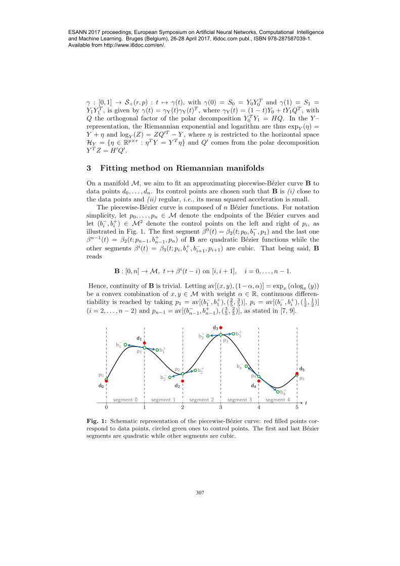
On a manifold M, we aim to fit an approximating piecewise-Bezier curve B todata points d0, . . . , dn. Its control points are chosen such that B is (i) close tothe data points and (ii) regular, i.e., its mean squared acceleration is small.

The piecewise-Bezier curve is composed of n Bezier functions. For notationsimplicity, let p0, . . . , pn ∈ M denote the endpoints of the Bezier curves andlet (b−i , b

+i ) ∈ M2 denote the control points on the left and right of pi, as

illustrated in Fig. 1. The first segment β0(t) = β2(t; p0, b−1 , p1) and the last one

βn−1(t) = β2(t; pn−1, b+n−1, pn) of B are quadratic Bezier functions while the

other segments βi(t) = β3(t; pi, b+i , b

−i+1, pi+1) are cubic. That being said, B

reads

B : [0, n] → M, t �→ βi(t− i) on [i, i+ 1], i = 0, . . . , n− 1.

Hence, continuity of B is trivial. Letting av[(x, y), (1−α, α)] = expx (αlogx (y))be a convex combination of x, y ∈ M with weight α ∈ R, continuous differen-tiability is reached by taking p1 = av[(b−1 , b

+1 ), (

25 ,

35 )], pi = av[(b−i , b

+i ), (

12 ,

12 )]

(i = 2, . . . , n− 2) and pn−1 = av[(b−n−1, b+n−1), (

35 ,

25 )], as stated in [7, 9].

segment 0 segment 1 segment 2 segment 3 segment 4t|

0|1

|2

|3

|4

|5

d0

d1

d2

d3

d4

d5p0

b−1p1 b+1

b−2

p2 b+2

b−3 p3

b+3

b−4p4

b+4

p5

Fig. 1: Schematic representation of the piecewise-Bezier curve: red filled points cor-respond to data points, circled green ones to control points. The first and last Beziersegments are quadratic while other segments are cubic.

307

ESANN 2017 proceedings, European Symposium on Artificial Neural Networks, Computational Intelligence and Machine Learning. Bruges (Belgium), 26-28 April 2017, i6doc.com publ., ISBN 978-287587039-1. Available from http://www.i6doc.com/en/.

Ideally, we would like to compute B that minimizes

minpi,b

+i ,b−i

f(B) + λn∑

i=0

d2(pi, di), (2)

where f(B) is the mean squared acceleration of B. The parameter λ > 0 adjuststhe balance between data fidelity and the “smoothness” of B. Note that, whenλ → ∞, (2) corresponds to the interpolation problem in [9]. However, insteadof addressing directly this difficult optimization problem where the optimizationvariables are control points on M, we take a suboptimal route that consists infinding optimality conditions when M = R

r and then generalizing those condi-tions to an arbitrary Riemannian manifold. As mentioned in the introduction,we will investigate in further work whether a more demanding “optimal route”would be worth the effort in practical applications.

In the easy case where M = Rr, d(·, ·) is the classical Euclidean distance and

f(B) =

n−1∑i=0

∫ 1

0

‖βi(t)‖2dt

Under continuity and differentiability constraints, the cost minimized in (2) isa quadratic function in the 2n variables p0, (b

−i , b

+i )

n−1i=1 and pn. Therefore, the

optimality conditions take the form of a linear system (A0 + λA1)x = λCd,where A0, A1 ∈ R

2n×2n and C ∈ R2n×n+1 are matrices of coefficients, x =

[x0, x1, . . . , x2n−1]T := [p0, b

−1 , b

+1 , . . . , b

+n−1, pn]

T ∈ R2n×r contains the 2n opti-

mization variables and d := [d0, . . . , dn]T ∈ R

n+1×r contains the data points.This problem is equivalent to x = λ(A0 + λA1)

−1Cd = Q(λ)d, or to

xj =∑n

l=0 qjl(λ)dl. (3)

Since the problem is invariant under translation, we have∑n

l=0 qjl(λ) = 1 for allλ. In other words, the unknown control point xj can be seen as an affine combi-nation of the data points dl. This also means that xj−d�j =

∑nl=0 qjl(λ)(dl−d�j ),

by translation with respect to a reference point d�j . As the Euclidean differencecan be seen as a logarithm map on a general manifold M, a simple and naturalway to generalize (3) to M is to (i) use the Riemannian logarithm to map thedata to the tangent space at the reference point d�j , (ii) compute the weighedmeans in the tangent space, and finally (iii) use the Riemannian exponential tomap the obtained points back to the manifold M. This yields

xj = expd�j

(n∑

l=0

qjl(λ)logd�j(dl)

). (4)

Observe that we recover (3) when M = Rr: indeed, we obtain xj = d�j +

(∑n

l=0 qjl(λ)(dl − d�j )), where d�j cancels out. This cancellation does not occurin general on nonlinear manifolds; by default, we choose d�j := di for xj being a

control point b−i , b+i or pi.

Finally, the curve B is reconstructed using the De Casteljau algorithm (asmentioned in Section 2).

308

ESANN 2017 proceedings, European Symposium on Artificial Neural Networks, Computational Intelligence and Machine Learning. Bruges (Belgium), 26-28 April 2017, i6doc.com publ., ISBN 978-287587039-1. Available from http://www.i6doc.com/en/.

4 Numerical results

θi

building

Fig. 2: Given a prevailing windθi, local wind orientation mightchange among the domain, spe-cially when an object (here a build-ing) perturbs it.

Now, we apply the proposed algorithm tothe wind field estimation problem (see Fig-ure 2). We work on a set of n = 33 covari-ance matrices C(θi) of size 3024 × 3024 ob-tained from unsteady CFD simulations andcorresponding to 33 prevailing wind orienta-tions θi = kπ/64, k ∈ {0, 1, . . . , 32}. For now,the magnitude of the wind field remains fixed,and further work will aim at extending our ap-proach to develop surface fitting tools, so thatboth the prevailing wind magnitude and ori-entation are allowed to vary simultaneously.Using a singular value decomposition, we re-duce the rank of C(θi) to r = 20 by factoriz-ing it as C(θi) � Y (θi)Y (θi)

T ∈ S+(20, 3024);hence Y (θi) ∈ R

3024×20∗ . Our algorithm is

implemented to directly work on the Y (θi),which has also the advantage of reducing thecomputational cost associated with basic matrix operations (notice that in thisapplication, it is not even necessary to build the matrix C(θi), and one caninstead obtain directly Y (θi) from the simulations).

We construct the piecewise-Bezier curve B(θ) ∈ S+(20, 3024) based on datafrom a training set ST = {C(θi)}i∈IT , where IT = {1, 3, 5, . . . , 33} and use theremaining data as a validation set SV = {C(θi)}i∈IV , with IV = {2, 4, . . . , 32}.We measure the fitting error of B(θ) compared to data from SΩ (Ω ∈ {T, V })as a relative mean squared error (MSE) in dB:

MSE(B(θ)) = 10 log

(∑i∈IΩ

||C(θi)−B(θi)||2F∑i∈IΩ

||C(θi)||2F

). (5)

We represent its evolution with respect to the parameter λ in Figure 3 (left).Not surprisingly, the MSE computed on the training set decreases when λ grows,as problem (2) is closer and closer to interpolation. Correspondingly, the MSEcomputed on the validation set at the limit λ → ∞ measures the model error,i.e., the inability of the piecewise-Bezier interpolation technique to recover thehidden data.

The main advantage of our method is its robustness to corrupted data. Toillustrate this, we artificially added some noise to the data. Consider a new

matrix C(θi) = C(θi)+0.05N(θi) with N(θi)lmiid∼ N (0, 1) for l,m = 1, . . . , 3024.

The corrupted matrices C(θi) are then factorized into C(θi) � Y (θi)Y (θi)T

similarly as above. This artificial noise results in an MSE(C(θ)) of about −9 dBcompared the (not corrupted) data points.

We compute the curve B(θ) based on the corrupted data from the set ST :={C(θi)}i∈IT and measure the MSE of B(θ) compared to the original data from

309

ESANN 2017 proceedings, European Symposium on Artificial Neural Networks, Computational Intelligence and Machine Learning. Bruges (Belgium), 26-28 April 2017, i6doc.com publ., ISBN 978-287587039-1. Available from http://www.i6doc.com/en/.

SΩ (Figure 3, right). We observe an optimal balance λopt between data fittingand curve smoothing with about 5 dB of MSE reduction compared to the noiselevel.

10−3 100 103 106−80

−60

−40

−20

0

training set

validation set

interpolation

λ

MSE

[dB]

No artificial noise on data

10−3 100 103 106

−15

−10

−5 training set

validation set

artificial noise

λopt

interpolation

5dB

λ

MSE

[dB]

With artificial noise on data

Fig. 3: Mean squared error (MSE) obtained on the training and validation sets,without (left) or with (right) additional noise on the data. When no noise is presenton the data (left), the error on the training set decreases with λ as the model tendsto interpolation. When noise is added to data (right), our method shows denoisingcapacities with up to 5 dB of MSE reduction compared to the noise level.

References

[1] L. Pyta and D. Abel. Interpolatory galerkin models for the navier-stokes-equations. IFAC-PapersOnLine, 49(8):204 – 209, 2016. 2nd IFACWorkshop on Control of Systems Governedby Partial Differential Equations CPDE, 2016.

[2] C. Samir, P.-A. Absil, A. Srivastava, and E. Klassen. A gradient-descent method for curvefitting on Riemannian manifolds. Foundations of Computational Mathematics, 12:49 – 73,2012.

[3] J. Su, I.L. Dryden, E. Klassen, H. Le, and A. Srivastava. Fitting smoothing splines to time-indexed, noisy points on nonlinear manifolds. Image and Vision Computing, 30(67):428 –442, 2012.

[4] P.-A. Absil, P.-Y. Gousenbourger, P. Striewski, and B. Wirth. Differentiable piecewise-Bezier surfaces on Riemannian manifolds. SIAM Journal on Imaging Sciences, to appear,2016.

[5] L. Machado and M. Teresa T. Monteiro. A numerical optimization approach to generatesmoothing spherical splines. Journal of Geometry and Physics, 111:71 – 81, 2016.

[6] G. Farin. Curves and Surfaces for CAGD. Academic Press, fifth edition, 2002.

[7] T. Popiel and L. Noakes. Bezier curves and C2 interpolation in Riemannian manifolds.Journal of Approximation Theory, 148(2):111–127, 2007.

[8] B. Vandereycken, P.-A. Absil, and S. Vandewalle. A Riemannian geometry with com-plete geodesics for the set of positive semidefinite matrices of fixed rank. IMA Journal ofNumerical Analysis, 33(2):481–514, 2013.

[9] A. Arnould, P.-Y. Gousenbourger, C. Samir, P.-A. Absil, and M. Canis. Fitting SmoothPaths on Riemannian Manifolds : Endometrial Surface Reconstruction and Preopera-tive MRI-Based Navigation. In F.Nielsen and F.Barbaresco, editors, GSI2015, 491–498.Springer International Publishing, 2015.

310

ESANN 2017 proceedings, European Symposium on Artificial Neural Networks, Computational Intelligence and Machine Learning. Bruges (Belgium), 26-28 April 2017, i6doc.com publ., ISBN 978-287587039-1. Available from http://www.i6doc.com/en/.