Preliminary—Comments welcome Pigou, Becker and the Regulation of Punishment‐Proof Firms Carl Davidson, Lawrence W. Martin, and John D. Wilson Department of Economics, Michigan State University; East Lansing, MI 48824 Revised, March 2012 Abstract : We study the use of fines and inspections to control production activities that create external damages. The model contains a continuum of firms, differing in their compliance costs, so that only high-cost firms evade the regulations. If fines are low, then Pigouvian rules for taxing externalities apply, modified to account for costly inspections. According to Becker’s classic work on crime and punishment, however, these inspection costs can be minimized by raising the fines to very high levels. But by bankrupting firms, high fines are shown to increase the external costs generated by a non-compliant firm’s production activities, although they reduce the number of firms that fail to comply with the regulation. We analyze this tradeoff in detail, and obtain some unexpected results about how it should be resolved.
Transcript
Preliminary—Comments welcome
Pigou, Becker and the Regulation of Punishment‐Proof Firms
Carl Davidson, Lawrence W. Martin, and John D. Wilson
Department of Economics, Michigan State University; East Lansing, MI 48824
Revised, March 2012
Abstract: We study the use of fines and inspections to control production activities that create external damages. The model contains a continuum of firms, differing in their compliance costs, so that only high-cost firms evade the regulations. If fines are low, then Pigouvian rules for taxing externalities apply, modified to account for costly inspections. According to Becker’s classic work on crime and punishment, however, these inspection costs can be minimized by raising the fines to very high levels. But by bankrupting firms, high fines are shown to increase the external costs generated by a non-compliant firm’s production activities, although they reduce the number of firms that fail to comply with the regulation. We analyze this tradeoff in detail, and obtain some unexpected results about how it should be resolved.
1
1. Introduction
Economic agents engage in a wide variety of activities that generate external effects. For
example, drivers impose congestion costs on others when they use public roads and may endanger
others by driving recklessly; homeowners may anger neighbors by listening to loud music or by
allowing their property to deteriorate; firms may generate hazardous waste as a byproduct of
production or expose their workforce to unnecessary health risks by not talking sufficient care in
designing their factories; and banks and other depositary institutions may accumulate the types and
quantities of assets that increase the risks of financial crises. Society responds to such situations by
attempting to regulating behavior and by punishing those who violate the established rules.
Sometimes the behavior is criminalized (it is illegal to dump hazardous waste), while in other
instances attempts are made to internalize the external damages (toll roads). In the economics
literature there are two classic treatments of the issues that surround such activity, due to Pigou
(1920) and Becker (1968), but the analyses differ in focus, and they offer solutions that have starkly
different tones. Our goal in this paper is to offer a new approach that unifies the messages of Pigou
and Becker by showing that the optimal policy prescription for activities that generate external costs
can take on either form, and identifying the conditions that determine which form it takes.
Pigou addressed the issue of externalities in The Economics of Welfare. An externality arises
whenever the social cost of an activity differs from the private cost. Pigou’s solution was to add a set
of taxes to the price mechanism that would force individuals to internalize the full social costs. Thus,
the Pigouvian solution is to set a tax which equals the marginal damage associated with the activity.
If the external cost of the activity is low, the Pigouvian tax will be low; whereas activities that
generate large external costs will be subject to large Pigouvian taxes. In this sense, the policy
prescription proposed by Pigou is one in which the punishment fits the crime. Although Pigou
(1954) acknowledged that there will be informational problems both in designing the optimal tax
2
scheme and implementing it, the issue of compliance played no role in his analysis. In addition,
Pigou’s analysis did not emphasize the illegal nature of non-compliance.
In contrast, the illegal nature of non-compliance is at the center of Becker’s (1968) analysis
of such issues in “Crime and Punishment: An Economic Approach.” Becker was interested in the
question of how society should go about enforcing laws that criminalize activities that generate
external costs. He focused on laws that are enforced by random inspection. The key policy
parameters are the probability of detection, adjusted by increasing the rate of inspection, and the level
of the fine imposed on those convicted of non-compliance. Becker’s goal was to find the optimal
policy; the one that minimizes the cost of the illegal activity.1 He argued that because detection is
costly while fines are nearly costless, the fine should be raised all the way up to the full wealth of the
perpetrator. This policy enables the regulation to be enforced with a low probability and low cost of
detection. It is important to note that in Becker’s world, it is optimal to set the fine at a very high
level, regardless of the costliness of detection and regardless of the extent of the external cost of the
activity. Thus, with Becker’s policy prescription, the size of the punishment does not necessarily fit
the crime – those found guilty of non-compliance are always driven to the edge of bankruptcy
regardless of the extent of the external damage.
It is clear that economists were uncomfortable with the counter-intuitive policy prescription
of drastically high fines and low audit rates put forth by Becker. In fact, this finding is sometimes
referred to as the “Becker conundrum” because we rarely observe such harsh punishment, even
though the argument in its favor is clear and compelling.2 Since 1968, over 200 articles have been
1 Becker recognized the need to correct marginal incentives. In fact, in the early part of his paper, he derived the optimal fine for a fixed inspection rate, showing that in the first-best outcome, the expected fine should be set equal to the harm (as noted by Polinsky and Shavell 2000, this result actually dates back to Bentham 1789). However, Becker’s focus was on enforcement. In particular, he argued that the existence of enforcement costs ensures that the marginal conditions that define the first-best outcome will not be satisfied. His solution of a high fine coupled with a low inspection rate was designed to minimize the distortions created by such costs. 2 In a survey of the literature on enforcement, Polinsky and Shavell (2000) provide a proof that the optimal fine is set at its upper limit when offenders are risk-neutral. Comparing this result with actual practice, they argue for
3
published on the economics of enforcement, with many targeted at conquering the Becker
conundrum.3 In contrast, the robustness of Pigou’s main result is rarely questioned.4 Extensions
have tended to focus on problems with implementation or complications that arise when Pigouvian
taxes co-exist with other taxes.5
In this paper, we argue that for certain regulations, Becker’s analysis is too narrow, in the
sense that it does not take into account the full implications of high fines. In particular, when firms
must borrow or rent capital to produce, but face regulations that are imperfectly enforced, high fines
may distort their choice of inputs and create inefficiencies in factor markets. The reason for this is
that if fines are high enough to bankrupt firms, they alter the effective cost of capital that firms face.
Bankruptcy eliminates the ability of the fine to depend on the firm’s capital usage, since the firm
knows that if it is caught evading the regulation, then it will pay all of its assets to the government
and investors, regardless of the size of the fine. If the external damages created by the firm’s
activities depend on its capital usage, then high fines may therefore increase these damages for each
non-compliant firm. In addition, the firm’s owners will realize that additional capital investment
cannot alter the assets available to them in the event of bankruptcy (none). Thus, the marginal cost
of capital is reduced by an amount that depends on the probability of detection and punishment.
higher fines. “Substantial enforcement costs could be saved without sacrificing deterrence by reducing enforcement effort and simultaneously raising fines.” 3 For example, harsh fines are not optimal if agents are risk averse (Polinsky and Shavell 1979), because high fines impose an additional risk-bearing cost. In addition, if illegal activities can take on different gradations, it is optimal to impose moderate fines on less serious violations, thereby maintaining sufficient marginal incentives to deter more serious offenses (Sandmo 1981). Other approaches concern the optimal treatment of self-reported violations (Innes 1999), the structure of the criminal justice system (Rubenfeld and Sappington 1987; Malik 1990; Andreoni 1991; and Acemoglu and Verdier 2000), and heterogeneity among offenders (Babchuck and Kaplow 1993). 4 For important exceptions, see Buchanan (1969), Carlton and Loury (1980, 1986) and Kohn (1986). In addition, as is well known, Coase (1960) argued that when transactions cost are low, Pigouvian taxes will not be needed to reach an efficient outcome. He argued that as long as property rights are well defined, economic agents will be able to agree to the first-best outcome and split the surplus that will be created by eliminating distortionary behavior. 5 The double dividend literature stresses that in addition to correcting behavior, Pigouvian taxes generate revenue for the government. This creates a secondary benefit by allowing the government to reduce other taxes in the economy that may be creating distortions, but the modern literature has emphasized flaws in this argument (see, for example, Bovenberg and de Mooij 1994, Fullerton and Metcalf 1998, or Fullerton, Leicester and Smith 2010). The problems associated with collecting the information required to implement a Pigouvian tax (for example, measuring the true social cost) were stressed Baumol (1972) and a steady stream of related work has followed.
4
This consideration reinforces our argument that high fines may increase the external damages created
by a firm’s production activities.
The costs of these distortions from high fines must be balanced against the gains from using
high fines to reduce detection costs while increasing the share of firms that comply with the
regulation. Below we develop a model that allows us to investigate how this tradeoff should be
resolved. We identify conditions under which it is optimal to enforce some regulations with
moderate fines and likely detection—the “Pigouvian approach”—while for others, a “Beckerian
approach” is optimal, with fines that not only bankrupt some or all firms, but seize some or all of the
assets that are involved in the illegal activity.
The Pigouvian approach survives when there are high external costs related to the firm’s
capital usage, whereas the Beckerian approach is preferable when there are high external costs
related to output, regardless of capital intensities. Perhaps more surprising, the Beckerian approach
is also preferable when these output-related external costs are low, provided capital-related external
costs are unimportant.
Other results are also potentially surprising. In particular, we find that low unit costs for
inspecting and detecting evasion of regulations do not necessarily justify the Pigouvian approach,
although this approach tends to rely heavily on inspection activities, to keep fines below levels that
would bankrupt firms. The basic insight is that low inspection costs may lower the resource costs
involved in maintaining a particular compliance level, but they do not increase the maximum feasible
level of compliance in our model.
While intuition might suggest that high fines should be avoided when firms’ demands for
capital are highly elastic, given the capital distortions described above, we show that the conditions
under which it is optimal for fines to bankrupt at least some non-compliant firms do not depend on
the capital demand elasticity.
5
A related result is that there can exist optimal fines and inspection rates that that embody both
the Pigouvian and Beckerian approaches, in the sense that some non-compliant firms are bankrupted
but fines, but not others, although the only innate differences between firms in our model is
differences in compliance costs. This finding does not mean that fines are at “intermediate levels.”
In fact, we show that if some or all non-compliant firms should be bankrupted by fines, then the fines
should seize all of their assets, leaving nothing to investors. Rather, other aspects of the fine and
inspection policies are adjusted to induce some firms to risk bankruptcy, such as higher fines on
detected evaders who have sufficient assets to remain solvent.
Finally, the Becker conundrum survives in unexpected cases in our model. When external
damages are low, we find that it is optimal to set fines high enough to not only bankrupt some firms,
but seize all of their assets; that is, “minor nuisances” should be addressed with low inspection costs
and very high fines, as a means of saving in inspection costs.
In the next section, we use a simplified version of our model to illustrate how bankruptcy
alters firm investment behavior in the presence of regulation and punishment. Our central concern is
with the structure of fines and inspection rates, but the government can employ a sales tax to offset
potentially undesirable impacts of fines and inspections on equilibrium output. Section 3 describes
the optimal policy under the constraint that fines are kept low enough not to bankrupt any firms -- the
Pigouvian approach. Section 4 describes the equilibrium when fines do create bankruptcies -- the
Beckerian approach -- and Section 5 demonstrates that if the government uses such fines, then they
should be set high enough to take all of a bankrupt firm’s assets, but not necessarily high enough to
bankrupt all firms. Sections 6-8 then provide a detailed exploration of the optimal choice between
the two approaches. Examples are provided in Section 9.
6
2. Framework
Our model consists of a perfectly competitive industry, in which firms finance capital on a
competitive market for loans. These firms face a government-imposed regulation of some sort. Our
model is set up to allow for a wide variety of regulations, including but not limited to, those that
restrict the type and quantity of capital (we provide some examples of appropriate regulatory settings
in Section 9). Compliance is costly, and we assume that the cost of compliance varies across firms.
In equilibrium, some firms choose to comply with the regulation, whereas other firms operate
illegally, risking detection and punishment, by evading the regulation. Neither the government nor
potential investors can observe the firm’s behavior (or its cost of compliance) without monitoring, so
investors cannot condition their investment decisions on the legal status of the firm.6 The
government enforces the regulation by randomly inspecting firms and fining evaders. A firm’s
capital is observed by the government’s auditor, so the fine will be allowed to vary with capital usage
in our formal model. But for illustrative purposes, we assume a fixed fine in this section. The
government’s goal is to set the regulation parameters (the inspection rate, fines and possibly taxes) in
a manner that maximizes social welfare.
We assume that each risk-neutral firm produces a single unit of output (x) using two inputs,
entrepreneurial activity (e) and capital (k), according to a production function, , , with neo-
classical properties. Capital is provided by investors, who are promised that after all markets clear,
they will be repaid the principal of the loan along with interest at rate r. The principal consists of the
6 Since the market for loans is competitive, all banks earn zero profits. Borrowers are able to obtain loans from multiple sources, and banks cannot increase profits by undertaking the costly activities needed to ascertain the borrower’s production plans. We ignore the effects of corporate and personal taxes on the cost of capital. In the absence of these considerations, the analysis does not depend on whether firms finance capital with equity or debt. In the case of equity financing, r becomes a required return on equity that firms must pay if they are not bankrupt. If firms use both debt and equity at the margin, then the required returns may differ, if bankruptcy reduces payments to debt holders, but not equity holders. We avoid this complication, since it would require that we develop a theory of the firm’s financial structure.
7
unit of capital, which does not depreciate, and the cost of a unit of entrepreneurial activity is
normalized at one.
The firm’s ability to repay investors will be determined by its choice of inputs, its behavior
with respect the law, and the size of the potential punishment. In particular, since entrepreneurial
assets are the residual claimants, the firm will have assets of to pay principal, interest and
fines, where p denotes the price of the product. If an evading firm chooses an input mix that ties up
its liquidity, then the fine is paid first and any remaining assets go to investors. If investors receive
less than the principal and interest owed to them, the firm is said to be “bankrupt.” Evading firms
that leave themselves with more liquidity may be able to pay large fines without bankruptcy.
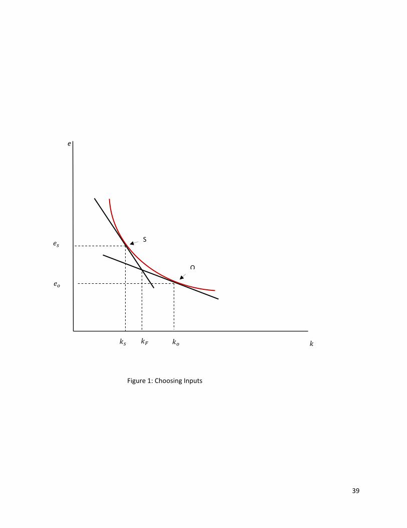
The firm’s input decision is depicted in Figure 1 with the convex curve representing the unit
isoquant. For law-abiding firms, the isocost curve is a straight-line with a slope of and, as is
usual, the firm minimizes costs at the tangency of the two curves. These firms always use an
efficient mix of inputs if r equals the social opportunity cost of capital (denoted by ∗). Things are
somewhat different for evaders; for them, the slope of the isocost curve will also depend on the
regulation parameters. To see this, note that for any given level of the fine, F, there exists a critical
level of capital, ≡ , such that an evader that selects will be bankrupt by the fine if
caught violating the law. This firm will realize that it’s effective cost of capital changes at . If the
firm selects , then it will carry sufficient liquidity to pay the fine and fully repay investors
regardless of circumstances. In this range, the firm’s effective cost of capital is the same as it is for a
law-abiding firm, r. However, if the firm selects , it will fully compensate investors when it
successfully evades the law, but it will be able to pay investors only the amount if fined.
If we use to denote the inspection rate, then the marginal cost of capital for evaders is 1 for
. The basic idea is that increasing k a unit, financed with borrowing, provides the firm with
another unit of assets to pay back principal, but there are no additional assets to pay interest in the
8
event the firm is fined; investors receive no interest income with probability . 7 A higher inspection
rate lowers this marginal cost because it increases the probability that the interest on additional
investment is effectively paid by the government through reduced fine payments, at no additional
cost to the firm. As a result, the isocost curve facing an evader is kinked, with a slope of for
and – 1 for . Since the kink occurs at , it will never be optimal for the firm
to use the level of capital that leaves it exactly bankrupt when fined.
Figure 1 illustrates the case where an evading firm is indifferent between choosing low and
high levels of k. In other words, the kinked isocost curve has two tangencies with the isoquant, one
on each side of the kink. More generally, when the when the fine is low, the kink occurs at a low
value for k, and it is optimal for the firm to operate on the steep portion of the isocost curve, at a
point such as S in Figure 1 (S for ‘solvent’). However, when the fine is high, the kink occurs at a low
value of k, and the firm will operate along the flatter portion of the isocost curve, at a point such as O
(O for ‘overleveraged’). In other words, a high enough fine lowers the marginal cost of capital from
r to 1 , causing the firm to increase its capital from to , and insuring bankruptcy in the
event of an inspection.
Thus, severe fines can significantly increase capital usage, resulting in large social costs,
particularly if greater capital usage increases external damages from the firm’s production activities.
Our formal model allows the government to base its fines on how much capital is employed by the
firm, but this is not helpful in the case of fines high enough to bankrupt the firm, because all of the
firm’s assets are lost, creating a fixed maximum punishment. Nevertheless, our analysis will show
that high fines are desirable in a variety of circumstances.
7 To be precise, for any given F, the expected cost of producing one unit of output is when and
1 when . Thus, the marginal cost of capital is r for and 1 for .
9
3. Pigouvian Regulation
We are now ready to begin our formal analysis, which we divide into three parts. First, in
this section, we confine our attention to situations in which the government finds it optimal to use
low or modest fines, so that evading firms are not driven to bankruptcy if caught. In the next two
sections, we consider the case of severe fines, and, finally, in Sections 6-8 we compare the two
outcomes to find the globally-optimal enforcement mechanism.
Each of our perfectly competitive firms employs entrepreneurial activity e and capital k to
produce a unit of output. The regulation both restricts k to some socially-optimal level, ∗, and
requires that firms reduce any external costs associated with production. In general these external
costs will depend on both the level of k and on the regulations involving the production process (e.g.,
emission controls in the case of pollution or restrictions on the use of particular financial instruments
in the case of financial firms). But to simplify the analysis, we assume that firms that comply with
the regulation produce no external costs, whereas those who evade the regulation generate
units of “external activity”. If the total output of the private good produced by non-compliant firms
is , then total external output is ≡ , which generates an external cost equal to ,
where h is strictly convex. In other words, external costs are allowed to depend on both capital usage
and output.
Firms are identical in all aspects except one, the cost of compliance. We use to denote a
firm’s cost of complying with the regulation, and we assume that this firm-specific parameter is
drawn after the firm enters the market from a continuous distribution function, denoted by .
Since a complier, or “legal firm,” generates no external costs, it is always socially optimal for this
firm to choose its capital and entrepreneurial inputs to minimize costs at the social opportunity cost
of capital, denoted ∗. Letting ℓ∗ denote this minimized costs, the total cost of production and
compliance is ℓ∗ for a legal firm with compliance cost .
10
Evaders choose their own capital levels and do not incur compliance costs, but they risk
detection and punishment. The probability of detection is the inspection rate, , which is the same
for all firms. The total fine depends linearly on the firm’s capital, , defined over all k that are
low enough for the fine not to bankrupt the firm. We will later argue that it is desirable to depart
from this linear structure once k reaches the level at which the linear fine and capital payments
exhaust all of the firm’s assets. Thus, the expected total cost for an evader firm is ,
where r is the interest rate that investors charge the firm, and the cost of capital now includes the
expected marginal fine on capital (the sub-script n indicates that this is the cost function for a non-
compliant firm). We assume that investors obtain capital at the economy-wide rate (opportunity
cost) of ∗. In the Pigouvian equilibrium, firms that evade the regulation choose to carry enough
liquidity to repay investors fully, in which case investors charge all firms the interest rate ∗.
A firm that is indifferent between complying and not complying with the regulation has a
compliance cost, , that satisfies
(1) ∗ℓ∗
All firms with prefer to operate legally; and all firms with prefer to evade the
regulation.
To complete the model, we now describe the timing of decisions. In the initial stage, ex ante
identical firms decide whether to enter the market. In stage two, is revealed and firms make their
input and compliance decisions. In particular, they decide on the mix of entrepreneurial and capital
inputs, and obtain funding from investors. These two stages may be viewed as occurring towards the
beginning of a period; investors must wait until the beginning of the next period to be paid. During
the period, the capital is put in place. The remaining stages then occur towards the beginning of the
next period. In stage 3, output is produced and sold, using the capital and entrepreneurial inputs, and
the regulatory authority randomly inspects firms, detects non-compliance, and assesses fines, which
11
must be paid immediately. In stage 4, investors are paid and entrepreneurs receive any remaining
assets. The crucial assumption here is that the government collects fines before investors are paid.
If the fine is set at a high level, then there may not be sufficient assets available to repay the investors
if the firm is detected cheating.
We solve the model by backwards induction. The solution the firm’s compliance decision is
as determined by (1). For the entry decision, since the firms do not know their value of before
entry, their expected profits from production are given by
(2) Π ℓ∗ ,
where p is the price of the product, is a sunk cost of entry, and is the maximum value of
among firms that produce.8 For any given set of enforcement parameters (T, t and ), there is a
unique value of p at which expected profits are zero. For all higher p, all firms enter and there will
be excess supply in the product market; for all lower p, no firm produces. Solving Π 0 for p
and using (1) yields the market-clearing price:
(3) ℓ∗ 1 .
We assume that the government also collects revenue from consumers by imposing a sales tax of
on this good, so that the price paid by consumers for each unit is ≡ . The assumption here is
that while some firms evade the regulation, all firms pay the tax. For example, a regulation
concerning a production process may be evadable, while no good possibilities exist for selling the
product without paying a sales tax.9
8 For simplicity, we assume that is low enough so that all firms that enter the market choose to produce when they learn their . Setting fixed cost sufficiently high will raise the equilibrium price p to insure that this assumption holds, given any . We may then also assume that the maximum feasible punishment never causes all firms to comply. 9 For analyses of the welfare effects of activities undertaken to evade taxes, see Davidson et al. (2005, 2007).
12
On the demand side of the product market, the representative consumer has the following
quasi-linear utility function:
(4) , ,
where I denotes the consumer’s lump-sum income and x is total output.10 Income I consists of an
endowment of the numeraire good, plus a government transfer financed by tax revenue and fines.
The consumer treats as fixed and chooses x to maximize utility. Thus, x satisfies the following
first order condition,11
(5)
Summarizing the product market, the producer price of output, p, is determined by the free-
entry condition and is given by (3). Total output, x, is determined by the sales tax and the solution
to the consumer’s maximization problem, given by (5). Since each firm produces one unit of output,
x also denotes the number of firms with 1 of these firms evading the regulation.
If evaders choose a relatively low level of capital (so that they carry enough liquidity to fully
repay investors in all cases), their expected costs are ∗ , as previously discussed. But
a higher level of capital (as depicted by point O in Figure 1) results in expected total costs of
1 ∗ , since the fine bankrupts the firm.12 As described in the previous section, the
higher level of capital entails a lower effective cost of capital and leads to a lower payment by the
firm when caught evading the regulation. It is important to note that the expected marginal fine on
capital, , no longer enters the cost of capital. Evaders who are not inspected pay no fine, and
evaders who are inspected surrender all of their assets to the government and investors. A rise in k
10 Production by law-abiding firms creates no external costs because these firms comply with the regulation. 11 We assume that I is large enough that (5) is satisfied for all relevant q. 12 At point O in Figure 1, the firm pays to entrepreneurs, 1 to capital owners, including principal, when not inspected (which occurs with probability 1 ) and to capital owners, when inspected (which occurs with probability ). Thus, expected production costs at O (excluding principal) are 1
. In addition, the firm faces an expected fine of . Summing to get total expected costs, we obtain 1 1 .
13
may increase the amount owed to the government, but the firm does not care about the split of its
assets between investors and the government; costs would not change if the government were given
all of the firm’s assets, leaving investors with none.
For the lower level of capital to be optimal for the firm, as required for a Pigou equilibrium, it
must lead to lower or the same expected costs, which occurs when
(6) ∗ 1 ∗
Thus, bankruptcy will not occur in equilibrium if (6) is satisfied by the government’s chosen
regulation parameters. We refer to (6) as the “Pigou constraint.”
We now turn to the government’s problem of optimal enforcement. In addition to the
external cost of , the government must also be concerned about the resources that it devotes to
enforcement. This cost is given by , where denotes the cost of inspecting one firm and is
the total number of inspections that are carried out. Social welfare (W) is given by
(7) ℓ∗ ∗ 1
where 1 and ∗ ∗ ; that is, the
asterisk indicates that we are evaluating the evader’s profit-maximizing inputs at the social
opportunity cost of capital [ ∗ for legal firms and ∗ ′ β) for evaders]. We assume that lump-
sum transfers are available to balance the government budget. Using (1) and (3), we may rewrite the
Pigou constraint, given by (6), as follows:
(8) ℓ∗ 1 σ ℓ
∗ 1 ∗ .
The government’s problem is to select the policy variables , , and τ to maximize social
welfare, subject to the Pigou constraint and the market equilibrium conditions. But the equilibrium
conditions have already been used to state the problem as the maximization of (7), subject to (8).
Note first that the fine T does not appear in the problem. Rather, it is replaced with the marginal
14
compliance cost, , as a control variable. Second, the sales tax is replaced by output x. Thus, the
control variables are , , , and x. After solving for their optimal values, we can return to the
equilibrium conditions and find the values of T and τ that support the equilibrium.
Maximizing (7) over x yields the following first-order-condition
(9) 1 ℓ∗ ∗ 1 0
where, to shorten notation, we have defined , ∗ ∗ , and ∗ with
the sub-script s used to reflects that the firm is solvent at this level of k. If we use (5) to substitute for
, (3) to substitute for p, and then solve for τ, we obtain
(10) 1 .
The tax is positive for two reasons. First, when another firm produces, expected inspections rise,
with an expected cost equal to . Second, the additional firm generates an expected external cost
equal to 1 , where 1 is the probability that the entrant will fail to comply
with the regulation. But there is a decline in expected total compliance costs equal to 1 . We
show below that the excess of this external cost over the reduced compliance cost is positive when
inspections are costly. Hence, a positive sales tax is needed to internalize this excess external cost,
plus the additional inspection cost.
Note next that the marginal fine on capital, t, enters only the objective function. Thus, we
may differentiate the objective function with respect to t, and obtain the following first-order
condition:
(11) β
This is the usual Pigouvian rule: the tax on another unit of an externality-producing activity should
equal the marginal external cost from that activity. Here the activity is additional investment. Note
that inspection costs do not alter the rule, because t can be adjusted without altering the total number
15
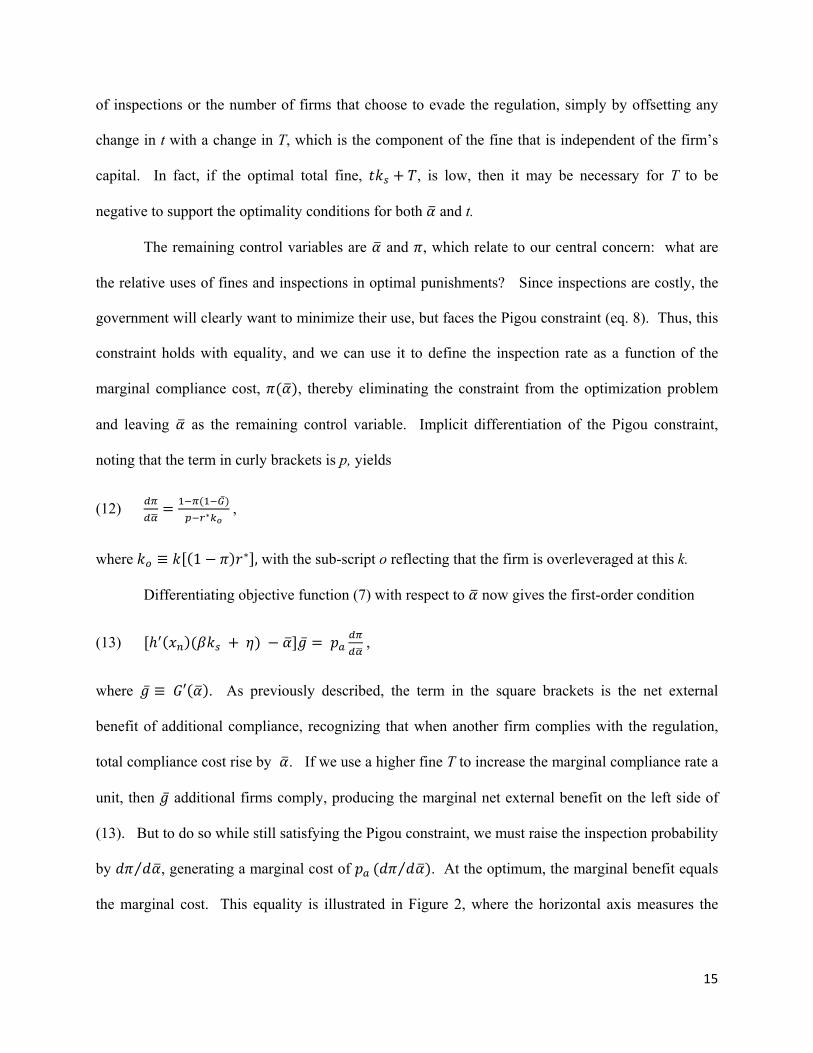
of inspections or the number of firms that choose to evade the regulation, simply by offsetting any
change in t with a change in T, which is the component of the fine that is independent of the firm’s
capital. In fact, if the optimal total fine, , is low, then it may be necessary for T to be
negative to support the optimality conditions for both and t.
The remaining control variables are and , which relate to our central concern: what are
the relative uses of fines and inspections in optimal punishments? Since inspections are costly, the
government will clearly want to minimize their use, but faces the Pigou constraint (eq. 8). Thus, this
constraint holds with equality, and we can use it to define the inspection rate as a function of the
marginal compliance cost, , thereby eliminating the constraint from the optimization problem
and leaving as the remaining control variable. Implicit differentiation of the Pigou constraint,
noting that the term in curly brackets is p, yields
(12)
∗ ,
where ≡ 1 ∗ , with the sub-script o reflecting that the firm is overleveraged at this k.
Differentiating objective function (7) with respect to now gives the first-order condition
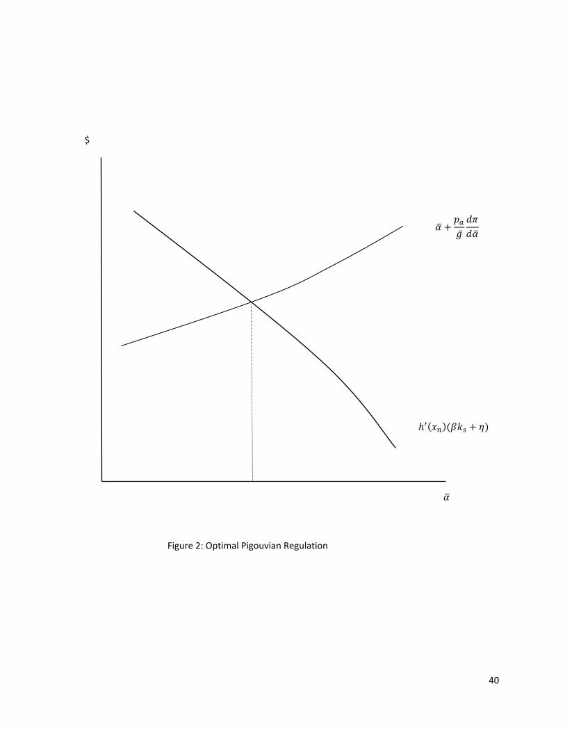
(13) ,
where ≡ ′ . As previously described, the term in the square brackets is the net external
benefit of additional compliance, recognizing that when another firm complies with the regulation,
total compliance cost rise by . If we use a higher fine T to increase the marginal compliance rate a
unit, then additional firms comply, producing the marginal net external benefit on the left side of
(13). But to do so while still satisfying the Pigou constraint, we must raise the inspection probability
by ⁄ , generating a marginal cost of ⁄ . At the optimum, the marginal benefit equals
the marginal cost. This equality is illustrated in Figure 2, where the horizontal axis measures the
16
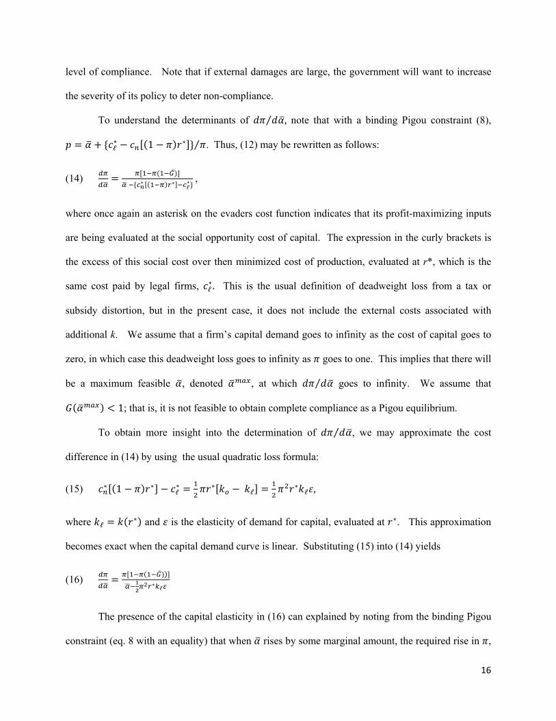
level of compliance. Note that if external damages are large, the government will want to increase
the severity of its policy to deter non-compliance.
To understand the determinants of ⁄ , note that with a binding Pigou constraint (8),
ℓ∗ 1 ∗ ⁄ . Thus, (12) may be rewritten as follows:
(14)
∗ ∗ℓ∗ ,
where once again an asterisk on the evaders cost function indicates that its profit-maximizing inputs
are being evaluated at the social opportunity cost of capital. The expression in the curly brackets is
the excess of this social cost over then minimized cost of production, evaluated at r*, which is the
same cost paid by legal firms, ℓ∗. This is the usual definition of deadweight loss from a tax or
subsidy distortion, but in the present case, it does not include the external costs associated with
additional k. We assume that a firm’s capital demand goes to infinity as the cost of capital goes to
zero, in which case this deadweight loss goes to infinity as goes to one. This implies that there will
be a maximum feasible , denoted , at which ⁄ goes to infinity. We assume that
1; that is, it is not feasible to obtain complete compliance as a Pigou equilibrium.
To obtain more insight into the determination of ⁄ , we may approximate the cost
difference in (14) by using the usual quadratic loss formula:
(15) ∗ 1 ∗ℓ∗ ∗ ℓ
∗ℓ ,
where ℓ∗ and is the elasticity of demand for capital, evaluated at ∗. This approximation
becomes exact when the capital demand curve is linear. Substituting (15) into (14) yields
(16)
∗ℓ
The presence of the capital elasticity in (16) can explained by noting from the binding Pigou
constraint (eq. 8 with an equality) that when rises by some marginal amount, the required rise in ,
17
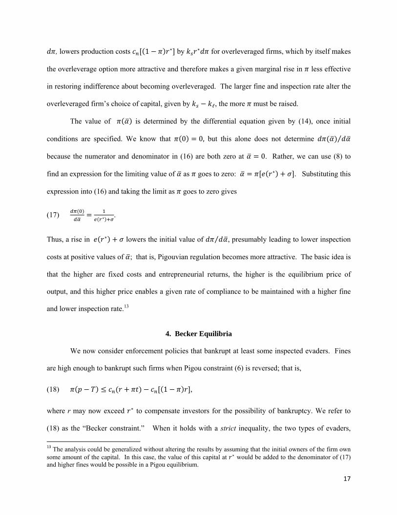
, lowers production costs 1 ∗ by ∗ for overleveraged firms, which by itself makes
the overleverage option more attractive and therefore makes a given marginal rise in less effective
in restoring indifference about becoming overleveraged. The larger fine and inspection rate alter the
overleveraged firm’s choice of capital, given by ℓ, the more must be raised.
The value of is determined by the differential equation given by (14), once initial
conditions are specified. We know that 0 0, but this alone does not determine ⁄
because the numerator and denominator in (16) are both zero at 0. Rather, we can use (8) to
find an expression for the limiting value of as goes to zero: ∗ . Substituting this
expression into (16) and taking the limit as goes to zero gives
(17) ∗ .
Thus, a rise in ∗ lowers the initial value of ⁄ , presumably leading to lower inspection
costs at positive values of ; that is, Pigouvian regulation becomes more attractive. The basic idea is
that the higher are fixed costs and entrepreneurial returns, the higher is the equilibrium price of
output, and this higher price enables a given rate of compliance to be maintained with a higher fine
and lower inspection rate.13
4. Becker Equilibria
We now consider enforcement policies that bankrupt at least some inspected evaders. Fines
are high enough to bankrupt such firms when Pigou constraint (6) is reversed; that is,
(18) 1 ,
where r may now exceed ∗ to compensate investors for the possibility of bankruptcy. We refer to
(18) as the “Becker constraint.” When it holds with a strict inequality, the two types of evaders,
13 The analysis could be generalized without altering the results by assuming that the initial owners of the firm own some amount of the capital. In this case, the value of this capital at ∗ would be added to the denominator of (17) and higher fines would be possible in a Pigou equilibrium.
18
“overleveraged” and “solvent” (when fined) will always use different amounts of capital to minimize
their costs of production. In particular, as described in Section 2, overleveraged firms will use a
higher level of capital, because they realize that if they fined, the marginal capital will be costless.
Equilibria where at least some evaders are overleveraged are referred to as “Becker
equilibria.” We can also distinguish between partial and full Becker equilibria, depending on
whether some or all evaders are overleveraged. Partial Becker equilibria are possible when the
Becker constraint holds with equality, in which case < 1 denotes the positive fraction of firms that
are overleveraged. To summarize, 1 in a full Becker equilibrium, ∈ 0,1 in a partial Becker
equilibrium, and 0 in a Pigou equilibrium.
Note that an equality on the Becker constraint does not distinguish a partial Becker
equilibrium from a full Becker equilibrium. If (18) holds with a strict inequality, the resulting
absence of any solvent evaders (when fined) implies that lowering their fine through a reduction in T
has no real effects. Thus, any Becker equilibrium can be supported with a fine structure that leaves
firms indifferent about becoming overleveraged. This indifference may be illustrated in Figure 1.
Once capital equals the cutoff level kF, above which the firm is bankrupt, the only restriction on
where we set the fine at higher k is that it must be high enough to continue to bankrupt the firm.
Given market prices, a bankrupt firm does not care if the fine is increased, since the higher fine is
financed by reduced payments of interest or principal. For this reason, the Becker constraint does
not contain a fine for bankrupt firms. However, we next show that the specific value of the fine on
bankrupt firms still matters, because it affects the equilibrium interest rate.
When the government inspects an overleveraged evader, it will now lay claim to some
income owed investors in an attempt to collect the unpaid fines. These anticipated seizures will
distort the capital market and lead to a higher price of capital for the regulated market. In
equilibrium, the profits earned by investors from supplying capital to this industry must exactly offset
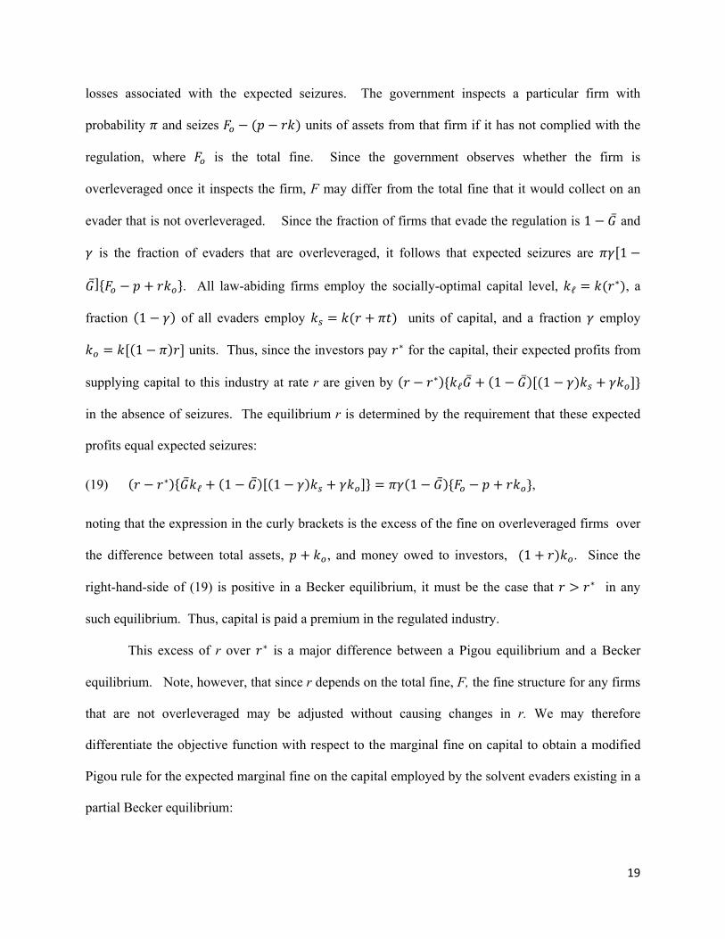
19
losses associated with the expected seizures. The government inspects a particular firm with
probability and seizes units of assets from that firm if it has not complied with the
regulation, where is the total fine. Since the government observes whether the firm is
overleveraged once it inspects the firm, F may differ from the total fine that it would collect on an
evader that is not overleveraged. Since the fraction of firms that evade the regulation is 1 and
is the fraction of evaders that are overleveraged, it follows that expected seizures are 1
. All law-abiding firms employ the socially-optimal capital level, ℓ∗ , a
fraction 1 of all evaders employ units of capital, and a fraction employ
1 units. Thus, since the investors pay ∗ for the capital, their expected profits from
supplying capital to this industry at rate r are given by ∗ℓ 1 1
in the absence of seizures. The equilibrium r is determined by the requirement that these expected
profits equal expected seizures:
(19) ∗ ℓ 1 1 1 ,
noting that the expression in the curly brackets is the excess of the fine on overleveraged firms over
the difference between total assets, , and money owed to investors, 1 . Since the
right-hand-side of (19) is positive in a Becker equilibrium, it must be the case that ∗ in any
such equilibrium. Thus, capital is paid a premium in the regulated industry.
This excess of r over ∗ is a major difference between a Pigou equilibrium and a Becker
equilibrium. Note, however, that since r depends on the total fine, F, the fine structure for any firms
that are not overleveraged may be adjusted without causing changes in r. We may therefore
differentiate the objective function with respect to the marginal fine on capital to obtain a modified
Pigou rule for the expected marginal fine on the capital employed by the solvent evaders existing in a
partial Becker equilibrium:
20
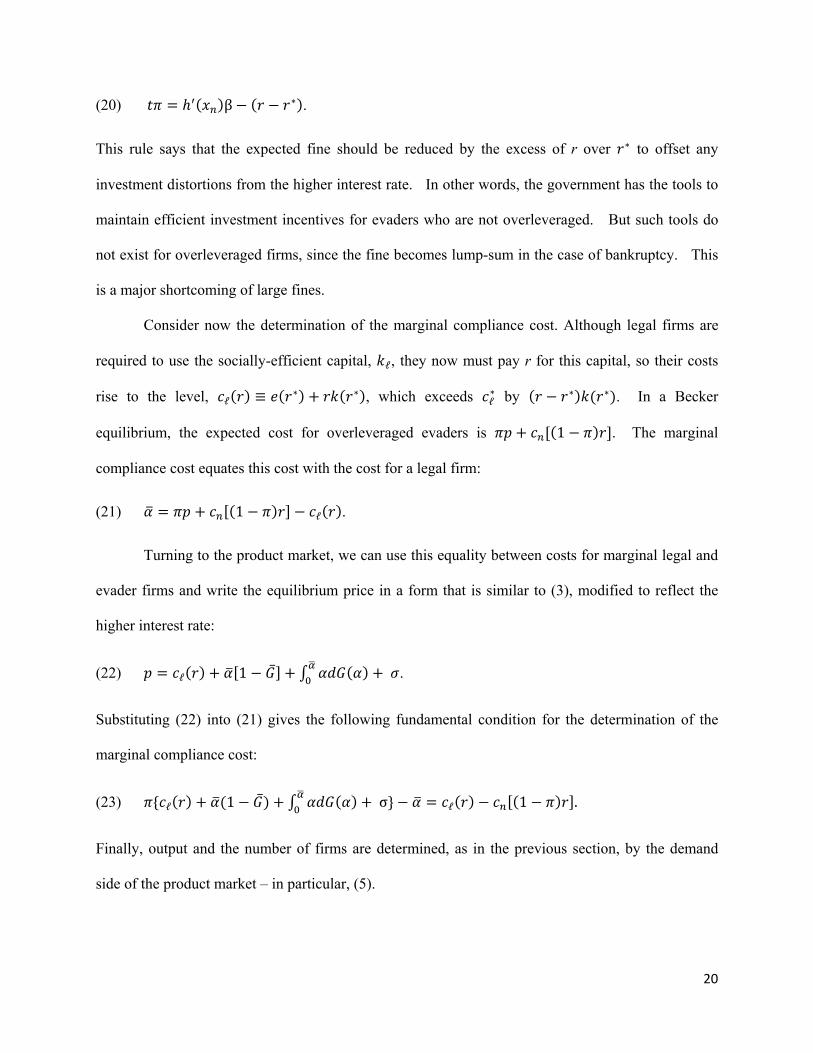
(20) β ∗ .
This rule says that the expected fine should be reduced by the excess of r over ∗ to offset any
investment distortions from the higher interest rate. In other words, the government has the tools to
maintain efficient investment incentives for evaders who are not overleveraged. But such tools do
not exist for overleveraged firms, since the fine becomes lump-sum in the case of bankruptcy. This
is a major shortcoming of large fines.
Consider now the determination of the marginal compliance cost. Although legal firms are
required to use the socially-efficient capital, ℓ, they now must pay r for this capital, so their costs
rise to the level, ℓ ≡ ∗ ∗ , which exceeds ℓ∗ by ∗ ∗ . In a Becker
equilibrium, the expected cost for overleveraged evaders is 1 . The marginal
compliance cost equates this cost with the cost for a legal firm:
(21) 1 ℓ .
Turning to the product market, we can use this equality between costs for marginal legal and
evader firms and write the equilibrium price in a form that is similar to (3), modified to reflect the
higher interest rate:
(22) ℓ 1 .
Substituting (22) into (21) gives the following fundamental condition for the determination of the
marginal compliance cost:
(23) ℓ 1 σ ℓ 1 .
Finally, output and the number of firms are determined, as in the previous section, by the demand
side of the product market – in particular, (5).
21
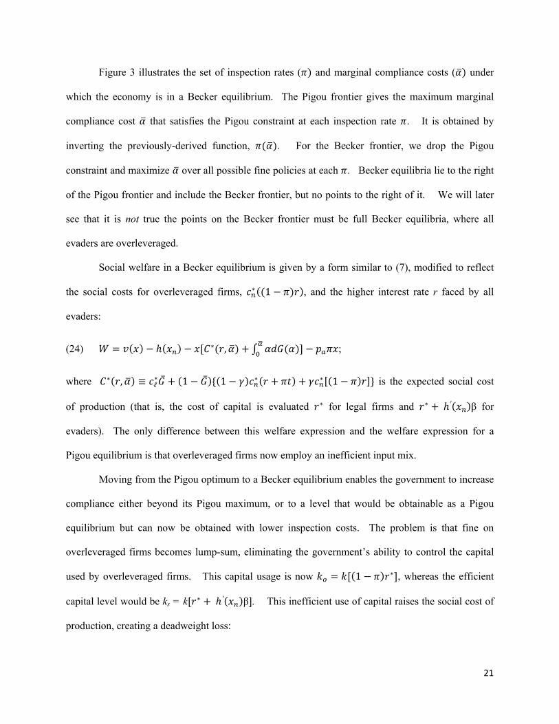
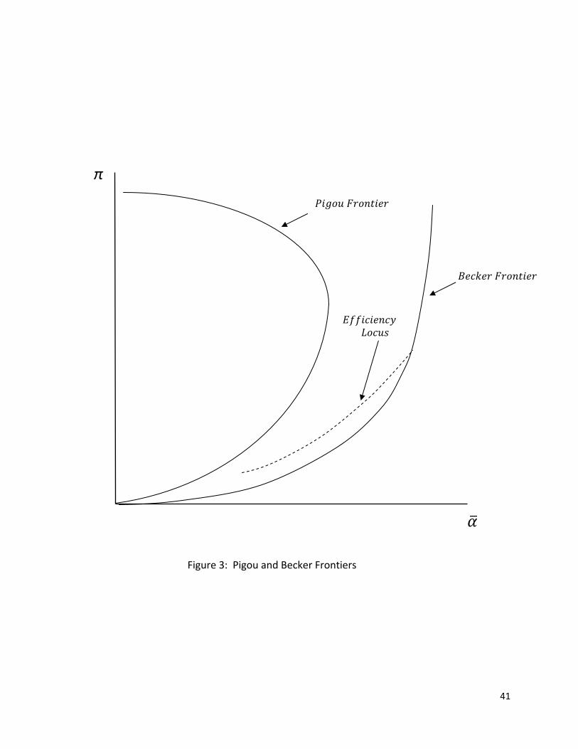
Figure 3 illustrates the set of inspection rates ( and marginal compliance costs ( under
which the economy is in a Becker equilibrium. The Pigou frontier gives the maximum marginal
compliance cost that satisfies the Pigou constraint at each inspection rate . It is obtained by
inverting the previously-derived function, . For the Becker frontier, we drop the Pigou
constraint and maximize over all possible fine policies at each . Becker equilibria lie to the right
of the Pigou frontier and include the Becker frontier, but no points to the right of it. We will later
see that it is not true the points on the Becker frontier must be full Becker equilibria, where all
evaders are overleveraged.
Social welfare in a Becker equilibrium is given by a form similar to (7), modified to reflect
the social costs for overleveraged firms, ∗ 1 , and the higher interest rate r faced by all
evaders:
(24) ∗ , ;
where ∗ , ≡ ℓ∗ 1 1 ∗ ∗ 1 is the expected social cost
of production (that is, the cost of capital is evaluated ∗ for legal firms and ∗ ′ β for
evaders). The only difference between this welfare expression and the welfare expression for a
Pigou equilibrium is that overleveraged firms now employ an inefficient input mix.
Moving from the Pigou optimum to a Becker equilibrium enables the government to increase
compliance either beyond its Pigou maximum, or to a level that would be obtainable as a Pigou
equilibrium but can now be obtained with lower inspection costs. The problem is that fine on
overleveraged firms becomes lump-sum, eliminating the government’s ability to control the capital
used by overleveraged firms. This capital usage is now 1 ∗ , whereas the efficient
capital level would be ks = k ∗ ′ β . This inefficient use of capital raises the social cost of
production, creating a deadweight loss:
22
(25) L = ∗ ′ β ∗ ′ β ∗ 1 ′ ,
where the second equality uses the quadratic loss expression for deadweight loss. This deadweight
loss represents the extra social cost involved in a move to a Becker equilibrium.
5. Optimal Fines in Becker Equilibria
Before investigating the desirability of moving to a Becker equilibrium, we investigate fines
in this type of equilibrium. In particular, we find that positive inspection costs are not sufficient to
overturn Becker’s conclusion that the fine should be maximized:
Proposition 1: Given any inspection rate π and marginal compliance cost that are supported by a
Becker equilibrium, welfare is maximized by setting the fine on overleveraged firms at its maximum
level, where the government takes all of the firm’s assets, leaving nothing for investors.
Proof: Suppose that the fine is less than its maximum level for overleveraged firms. Recall that we
can adjust the fine on solvent evaders to make them indifferent about becoming overleveraged. Then
we can raise the fine while lowering the share of evaders that are overleveraged, in a way that keeps
the equilibrium r fixed. With r fixed, there is no change in capital demands by overleveraged firms,
and so no change in deadweight loss per overleveraged firm; and there is no change in the
compliance level. But the fall in the share of evaders that are overleveraged implies lower total
deadweight loss, if overleveraged firms generate positive deadweight losses. In this case, welfare
rises. If deadweight losses are zero, there is no change in welfare. Q.E.D.
Thus, even for small policy changes from the Pigou optimum to a Becker equilibrium, it will
be optimal to raise the fine on some evaders -- the overleveraged firms -- to its highest possible level.
23
6. Is a Becker Equilibrium Better than the Pigou Optimum?
This section identifies conditions under which welfare can be improved by moving to a
Becker equilibrium. In particular, we consider small policy changes from the Pigou optimum that
create overleveraged firms, and we ask whether these changes increase welfare.
The introduction of overleveraged firms raises both and r, from 0 and ∗. But the
change in r does not directly cause any marginal distortions, because all existing firms in the Pigou
equilibrium are choosing their socially-optimal capital levels. Rather, only the increase in matters,
and it lowers welfare because each new overleveraged firm is creating the deadweight loss, L, by
using too much capital. The marginal welfare change per unit of output x is
(26) 1 .
The first and second terms also apply to the Pigou equilibrium and would be equated to zero if the
changes in and were required to satisfy the binding Pigou constraint. But now can be
increased with a lower increase in costly inspections. However, raising with fewer additional
inspections means a greater increase in fine, which generates the movement of some firms to the
overleveraged status. The third term in (26) gives the resulting welfare loss. Given our starting point,
ℓ 1 now denotes the average capital used by firms at the Pigou optimum.
Assuming that the capital demand curve is linear over the relevant region, which allows us to employ
the quadratic deadweight loss approximation in (26), we obtain:
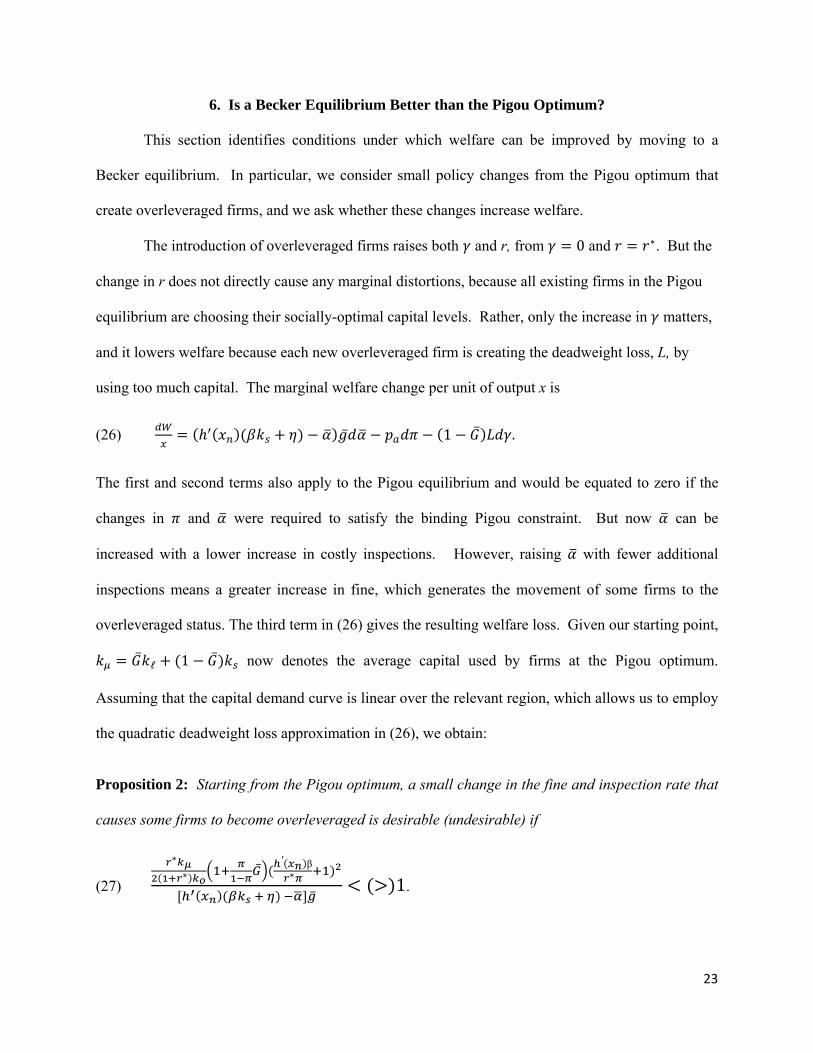
Proposition 2: Starting from the Pigou optimum, a small change in the fine and inspection rate that
causes some firms to become overleveraged is desirable (undesirable) if
(27)
∗
∗ ′ β∗
1.
24
Proof: Start with the optimal ( , , determined by (12) and (13):
(28) ;
∗ .
Next, implement a perturbation in the inspection rate and fine that involves increasing a marginal
unit, but with a rise in that is an amount less than the amount needed to remain in the Pigou
regime:
(29)
∗ ∗ℓ∗ .
With evaders indifferent about becoming overleveraged in the partial Becker equilibrium, the Becker
constraint (18) holds with equality, and (21) can be used to rewrite it in the same form as Pigou
constraint (8), modified to reflect a possible r > ∗:
(30) ℓ 1 ℓ 1 .
We may differentiate (30) to find the change in r from ∗ needed to keep evaders indifferent about
becoming overleveraged, following the changes in the expected fine and inspection rate satisfying
(29):
(31) ℓ
.
Differentiating the condition for capital market equilibrium, given by (19), we obtain the
marginal effect of a rise in r from ∗ on the fraction of firms that choose to become overleveraged:
(32)
∗ .
Multiplying (31) and (32) together then gives
(33)
ℓ ∗ .
25
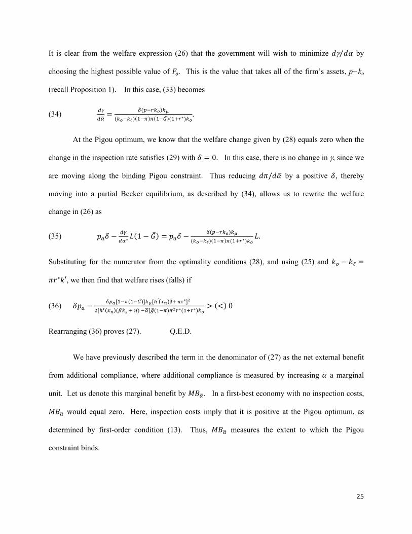
It is clear from the welfare expression (26) that the government will wish to minimize ⁄ by
choosing the highest possible value of . This is the value that takes all of the firm’s assets, p+ko
(recall Proposition 1). In this case, (33) becomes
(34)
ℓ ∗ .
At the Pigou optimum, we know that the welfare change given by (28) equals zero when the
change in the inspection rate satisfies (29) with 0. In this case, there is no change in , since we
are moving along the binding Pigou constraint. Thus reducing / by a positive , thereby
moving into a partial Becker equilibrium, as described by (34), allows us to rewrite the welfare
change in (26) as
(35) ∗ 1 ℓ
∗ .
Substituting for the numerator from the optimality conditions (28), and using (25) and ℓ
∗ ′, we then find that welfare rises (falls) if
(36) ′ β ∗
∗ ∗ 0
Rearranging (36) proves (27). Q.E.D.
We have previously described the term in the denominator of (27) as the net external benefit
from additional compliance, where additional compliance is measured by increasing a marginal
unit. Let us denote this marginal benefit by . In a first-best economy with no inspection costs,
would equal zero. Here, inspection costs imply that it is positive at the Pigou optimum, as
determined by first-order condition (13). Thus, measures the extent to which the Pigou
constraint binds.
26
On the other hand, the numerator of (27) is related to the costs involved in moving into the
partial Becker region. As increases, the market interest rate r rises to support the higher by
increasing the effective punishment of detected evaders who are overleveraged. But r must rise a lot
if the inspection rate is close to zero, because then ℓ, is small, indicating that the rise in r does
not “punish” evaders much more than legal firms. For this reason, dr/d is inversely proportional to
ℓ, and therefore inversely proportional to in the case of a linear capital demand function (see
eq. 31). In addition, dγ/dr is also inversely proportional to (see eq. 32). If there are few
inspections, then each overleveraged firm has only a small probability of not paying back investors.
Hence, there must be a large number of overleveraged firms to support an r above r*. Multiplying
these two derivatives together gives dγ/ , which is then inversely proportional to the square of .
Thus, lower leads to a higher rate at which the share of evaders who are overleveraged must rise as
the compliance level rises. On the other hand, a lower also reduces the deadweight loss generated
by each overleveraged firm. But even at 0,deadweight loss remains if β > 0, since increased
capital usage by overleveraged firms is then generating more external costs. The following
proposition reflects this tradeoff:
Proposition 3: For any pa > 0 and β>0, there exists a marginal compliance cost, ’ > 0, such that
if the economy is initially on the Pigou frontier at a positive < ’, then any marginal policy
change that creates overleveraged firms causes welfare to fall.
Proof: Assume that β>0. Equation (17) and optimality condition (28) show that the denominator
of (27) converges to a positive number as goes to zero, provided pa is positive, as assumed. For
β 0, the numerator of (27) goes to infinity as goes to zero, which happens along the Pigou
frontier as goes to zero. Thus, the left side of (27) exceeds the right side for sufficiently small ,
implying that welfare falls. Q.E.D.
27
Thus, if the Pigou optimum involves sufficiently low levels of compliance and capital-related
external costs are positive (β>0), then small policy changes that create overleveraged firms must
lower welfare. The Pigou optimum will have low levels of compliance if external costs are low or
unit inspection costs are high. In these cases, Proposition 3 tell us that it is not desirable to create a
small number of overleveraged firms. When we later consider policy changes that create greater
numbers of overleveraged firms, welfare improvements will be possible with low compliance levels
and positive values of β, but it will still be necessary to restrict the relative size of β.
Suppose next that external costs are high enough to move the Pigou-optimal marginal
compliance cost close to its maximum feasible level, denoted by . In this case, welfare
improvements from the Pigou optimum are also possible. 14
Proposition 4: For any pa >0 and ≥ 0, there exists a marginal compliance cost, ’ < , such
that if external cost parameter is large enough to imply a Pigou optimum with marginal
compliance cost between ’ and , then any marginal policy change from this optimum that
creates overleveraged firms must raise welfare.
Proof: Recall that 1. Since d / goes to infinity as goes to from below,
(28) shows that the marginal benefit term in the denominator of (27) also goes to infinity. But the
numerator of (27) stays bounded from above by some positive number. Thus, the expression in (27)
goes to zero, proving the proposition. Q.E.D.
Thus, creating some overleveraged firms is desirable if the external cost component
associated with output is high, since then there is a large benefit from being able to raise compliance
through the use of high fines. But restrictions must be placed on the relative size of the external cost
14 There are no similar results for a sufficiently low pa because reducing pa enough will produce a corner solution, where there is complete compliance at the Pigou optimum, and therefore no scope for increasing compliance. Moreover, it can be shown in this case there are no marginal changes in the fine and inspection rate that increase welfare by lowering compliance.
28
component that depends on capital, because the inability of fines to influence the capital usage of
overleveraged firms becomes increasingly costly as this component rises.
7. Efficient Becker Equilibria
We now show that in some cases there will exist Becker equilibria in which overleveraged
firms create no deadweight losses. The simple idea here is that the equilibrium r can increase so
much that it offsets the negative impact of the inspection rate in the cost of capital formula, leaving
deadweight losses equal to zero, as defined in (25). Whether this is possible will require that the
external costs associated with capital (β) be sufficiently small, since their presence raises the social
cost of capital. Also, there cannot be too few non-compliant firms, because then r need not increase
much to compensate investors for their bankruptcy risks. The result may be stated as follows:
Proposition 5: For sufficiently small values of the external cost parameter β, there exists an
interval, , ,with , such that any marginal compliance cost in this
interval is supported by an efficient Becker equilibrium (L = 0). As β goes to zero, 1(β) converges
to zero and 2(β) converges to a positive number. A full Becker equilibrium supports 2(β); that is,
all firms are overleveraged.
Proof: From capital-market condition (19), we may write:
(37) ∗ 1 1
,
where is the average capital used by all firms – that is, ≡ ℓ 1 1 .
Setting , so that the fine takes all of the firm’s assets, (37) becomes
(38) ∗ 1 1
.
29
At = 0 and 1, (38) becomes ∗ 1 . It is then clear that ∗ 1 0 for
positive that are sufficiently close to zero. If is not too high, we will then also have
∗ 1 0 for sufficiently close to zero. If we then lower below one, we can achieve
equality between ∗ and 1 for sufficiently close to zero (since lowering causes r
to fall and if we take to zero, r would equal ∗). As rises we can continue to find a that restores
this equality (from eq. 19), until some maximum is reached, at which point equality is obtained
with 1. It is then clear that and can be constructed with the properties in the
proposition. Q.E.D.
Thus, moving to a Becker equilibrium enables us to achieve greater compliance, with no
change in inspection costs and no deadweight losses from inefficient use of capital, if the initial level
of compliance is sufficiently low, and the capital-induced external cost ( is not too high.
Conditions for low compliance would include low external costs (both and η), or high unit
inspection costs. But this result gives us a type of “Becker conundrum”: the regulatory response to
actions by firms that involve low social costs should be to save on inspection costs by bankrupting
some firms and taking all of their assets. But this result requires the qualification that is
sufficiently low. For high , bankruptcy will be too costly from a social welfare viewpoint, because
then the fine can no longer induce firms to use socially-efficient levels of capital. The fundamental
problem is that large fines are necessarily lump-sum punishments, if they cause bankruptcy. In
particular, the amount of punishment no longer depends on the amount of capital.
A possible set of efficient Becker equilibria is illustrated in Figure 3 by the curve called the
“efficiency locus.” At each point on this curve, the cost of capital is the same for overleveraged and
solvent evaders. Thus, they choose the same capital and therefore have the same costs when they
are not inspected and fined. For any partial Becker equilibrium, they must then be equally well off
when detected and fined. The solvent firms are able to pay investors back in full, leaving no assets
30
for the firm owners, whereas the overleveraged firms pay a fine equal to the entire value of their
assets (Prop. 1). But the fine can no longer be uniquely determined by the level of capital, since all
evaders have the same capital. Thus, points on the efficiency locus are supported using a policy of
random fines, where the government chooses a fraction of firms γ to pay the high fine, with the
remaining evaders paying the low fine. Given the marginal compliance cost , this fraction is set so
that r rises to the level at which all evaders pay the social marginal cost of capital.
The location of the efficiency locus can be used to show that points on the Becker frontier
need not be full Becker equilibria. If is positive, then the socially-optimal cost of capital for
evaders should exceed the cost of capital for legal firms, since only the former create capital-related
external costs. But then legal firms use more capital than evaders, so an increase in r makes evasion
more attractive [see eq. 23 for the relation between r and ]. Thus, given π, the only way to get
from the efficiency locus to the higher compliance level on the Becker frontier is for r to fall, and this
is possible while maintaining equilibrium in the capital market (eq. 19) only if there are fewer
overleveraged firms. It follows that points on the Becker frontier to the right of the efficiency locus
are partial Becker equilibria, not full Becker equilibria. In other words, the level of compliance need
not be maximized by going to a full Becker equilibrium.
For points on the Becker frontier where compliance is sufficiently high and the inspection
rate approaches one, it will not be possible to raise r enough for 1 to equal or exceed ∗. In
this case, legal firms are always more capital-intensive than overleveraged firms, so the Becker
frontier is achieved with a full Becker equilibrium. We next ask whether such full Becker
equilibrium is optimal.
8. When is a Full Becker Equilibrium Optimal?
In this section, we derive conditions under which a full Becker equilibrium is optimal. In
particular, we shall consider cases where full Becker equilibria involve relatively high levels of
31
compliance, in which case they lie on the Becker frontier. In such cases, it seems intuitively
reasonable for a full Becker equilibrium to be desirable when increasing compliance generates large
social benefits. This turns out to be true, but with some qualifications that concern the cost side.
Any deadweight losses from moving to a full Becker equilibrium are given by 1 ,
where the deadweight loss L is defined in (25). Recall the quadratic approximation of this loss:
(39) ∗ 1 k′,
where k’ is the capital demand derivative. Since the “effective subsidy” on capital is squared in the
deadweight loss formula, large values of may imply a huge deadweight loss, relative to any gains
from using fines that bankrupt firms to raise beyond its maximum Pigou value. We then have a
tradeoff: going from the Pigou-optimal compliance level to a level in the Becker region reduces the
number of firms that are creating external costs, but by increasing the capital used by the non-
compliant firms, it increases the external cost per firm. If either or the capital demand elasticity
are low, then the latter consideration is unimportant, but a high capital demand elasticity may
actually raise external costs so much that for high , the Pigou optimum remains preferable to any
Becker equilibrium. This demand elasticity is not an issue in Proposition 2, because although it
increases the deadweight loss per firm, we also showed that it increases the rate at which firms
become overleveraged as rises, given by ⁄ , and the two effects cancel out. Since 1 at a
full Becker equilibrium, a higher capital elasticity increases the deadweight loss, without offsetting
effects.
Consider, for example, the 2-technique case illustrate in Figure 4, where the technique with
the low capital intensity is assumed to be socially efficient. Suppose that 0 and > 0. If the
capital intensities for the two techniques are sufficiently far apart, while the lower cost of capital
faced by non-compliant firms in the Becker region causes them to switch to the high capital-intensive
technique, then external costs will actually be higher in the Becker region than in the Pigou region.
32
On the other hand, similar intensities combined with a sufficiently high will ensure that a Becker
equilibrium is superior to the Pigou optimum.
If external cost depend only on the component of external cost not dependent on the capital
intensity ( 0; 0), then increasing this component enables us to increase the marginal benefit
of additional compliance, , while having no effect on deadweight
loss, L . Thus, sufficiently high and low β will ensure that a full Becker equilibrium is better than
the Pigou optimum. We provide a more formal statement of this result for the case of an iso-elastic
marginal damage function.
Proposition 6: Assume that the external damage function h is isoelastic. Then there exists positive
numbers ’ and δ, such that if external cost parameter is greater than ’, while external cost
parameter β satisfies , then the globally-optimal fine and inspection rate supports a full
Becker equilibrium, where all evaders are overleveraged.
Proof: The iso-elastic h function may be written as , 1; in which case
. Thus, the constraints on and β in the proposition place an upper bounds
on deadweight loss, L, under any given structure of fines and inspection costs. On the other hand
can be increased without bound by raising , insuring that increasing into the Becker region
will eventually increase social welfare. Q.E.D.
Finally, it is tempting to conjecture that a sufficiently low pa insures that the Pigou optimum
provides greater welfare than any Becker equilibrium, but this conjecture turns out to be wrong. The
problem is that the at which ⁄ goes to infinity does not depend on pa, so the maximum
that satisfies the Pigou constraint is independent of pa. If external costs are sufficiently high, it may
be desirable to achieve higher compliance levels, at any unit inspection cost, including zero.
33
9. Examples
While we believe that our model applies to a broad spectrum of regulated activities, ranging
from nuisances, such as product safety and illegal parking, to environmental, safety and financial.
Not all of these regulation settings accord perfectly with the framework described above. Minor
deviations may emerge if, for example, the regulation does not restrict the level of capital that firms
may use.15 Nevertheless, our main results with respect to the desirability of Pigouvian versus Becker
regulation will carry through provided that the key features of the model remain in place. The key
attributes of the model that we need are: a regulation that specifies some production technology, the
existence of alternative technologies, the rental of some portion of capital from investors, the
inability of investors to discern the legal status of their borrowers, random inspection and monetary
fines that potentially bankrupt evaders. In addition, violations of the regulation must generate
external costs that may depend upon the level of output, the type of capital or the amount of capital.
To provide some additional context for the analysis that follows, we close this section by providing
four concrete examples and with a brief description of how they satisfy the criteria needed to
generate our results.
Ex. 1: Illegal parking by delivery firms.
Consider an industry of restaurants that deliver meals to households. When parking the
delivery vehicle, the firm faces a regulation about where it may park legally. Generally, the costs of
compliance will vary with the availability of legal spaces, congestion, the character of the
neighborhood, and the type of delivery car used. Any firm that evades the regulation risks a
monetary fine, which, if high enough, could lead to bankruptcy and the seizure of assets by the
parking authority. Investors considering loaning vehicles or lending money to firms in this industry
15 If legal firms are free to use any level of capital, then an additional inefficiency arises in the partial Becker and full Becker cases since the increase in r above ∗ will cause legal firms to under-invest in capital. This additional distortion makes the welfare analysis slightly more complicated, by adding additional welfare losses that are tied to strict punishment, but it does not alter the basic message of this paper.
34
will demand a premium that compensates them for their expected losses. Firms that face bankruptcy
will perceive a lower marginal cost of capital and presumably substitute cheap capital for other
relatively expensive inputs. In this example, the external cost depends only upon the amount of
illegal parking. In order to reduce it, the government may use higher fines, more likely detection and
perhaps a tax on the activity itself. Since it is the production of output—meal delivery—not the
capital used to produce it—trucks, ovens, etc.—that produces the external cost, our analysis suggest
the optimality of high fines, rather than high detection rates, particularly if we view illegal parking as
belonging to the category of relatively “minor nuisances” (Proposition 5). This solution is based
solely on efficiency considerations and assumes risk-neutrality.
Ex. 2: Pollution regulation
Pollution regulations often require the installation of the “best available” pollution control
equipment to mitigate the damage from emissions. A firm can evade the regulation by choosing a
different technology. Depending upon the age of the plant, the complexity of the production process,
the firm’s experience and the skills of its workforce, the cost savings will vary (forgoing these
savings is equivalent , of course, to bearing the costs of compliance). High fines may expose the
firm to bankruptcy if detected with the non-compliant equipment, but, as we have seen, they lower its
marginal cost of capital, inducing the firm to use more capital-intensive production techniques than
those employed by legal competitors. This factor market distortion is a cost of the severe fine. In
addition, the external cost depends on the amount of non-compliant capital. If this particular cost is
high, then low fines and frequent inspections may be desirable, so that that the fine structure can be
adjusted to provide evaders of the regulation with the proper incentives to limit their capital usage.
On the other hand, if there is little substitutability in the use of capital, then such incentives are
unimportant (the deadweight loss L is low in our model), and high external costs then suggest the
35
use of high fines, particularly if high inspection costs make it costly to control pollution with low
fines.
Ex. 3: Licensing requirements
Many industries have licensing requirements. For example, hair salons must hire licensed
stylists. The licensing requirement typically specifies some minimal level of training (that is, a
minimum level of industry-specific human capital).16 Measure the human capital on the vertical axis
of Figure 1. Then a non-compliant firm will hire stylists with illegally low levels of training and
substitute other forms of capital, such as furniture, design and equipment, for the regulated human
capital. Facing potential bankruptcy, these firms borrowed funds at a rate of 1 and
operate at a point such as B in Figure 1. Lenders will not perceive the compliance or non-compliance
of the individual firm but will be aware that losses exist and demand the appropriate payment. The
external cost will not depend upon the capital, but rather upon only the level of output. Assuming
this external cost is not too high, Proposition 5 suggests the use of high fines.
16 In Michigan barbers must complete a 2,000 hour course of study. (Barbering Law Book, Michigan Department of Labor and Economic Growth, BCS-LDL-PUB-001 (02/06).
36
References
Acemoglu, Daron and Thierry Verdier (2000). “The Choice Between Market Failures and
Corruption.” American Economic Review 90: 194-211.
Andreoni, James (1991). “Reasonable Doubt and the Optimal Magnitude of Fines: Should the
Penalty Fit the Crime?” Rand Journal of Economics 22(3): 385-95.
Babchuk, Lucien and Louis Kaplow (1993). “Optimal Sanctions and Differences in Individual’s
Likelihood of Avoiding Detection.” International Review of Law and Economics 13: 217-
24.
Baumol, William (1972). “On Taxation and the Control of Externalities.” American Economic
Review 62(3): 307-22.
Becker, Gary (1968). “Crime and Punishment: An Economic Approach.” Journal of Political
Economy 76: 167-217.
Bentham, Jeremy (1789). An Introduction to the Principles of Morals and Legislation. In The
Utilitarians. Rept. Garden City, NY: Anchor Books, 1973.
Bovenberg, A. Lans and Ruud de Mooij (1994). “Environmental Levies and Distortionay Taxation.”
American Economic Review 84(4):1085-89.
Buchanan, James (1969). "External Diseconomies, Corrective Taxes, and Market Structures."
American Economic Review 59: 174-77.
Carlton, Dennis and Glenn Loury (1980). “The Limitations of Pigouvian Taxes as a Long-Run
Remedy for Externalities.” Quarterly Journal of Economics 95(3): 559-66.
Carlton, Dennis and Glenn Loury (1986). “The Limitations of Pigouvian Taxes as a Long-Run
Remedy for Externalities: An Extension of Results.” Quarterly Journal of Economics
101(3): 631-34.
Coase, Ronald (1960). “The Problem of Social Cost.” Journal of Law and Economics 3(1): 1-44.
37
Davidson, Carl, Lawrence L. Martin and John D. Wilson (2005). “Tax Evasion as an Optimal Tax
Device.” Economics Letters 86: 285-290.
Davidson, Carl, Lawrence L. Martin and John D. Wilson (2007). “Efficient Black Markets?” Journal
of Public Economics 91: 1575-1590.
Fullerton, Don and Gilbert Metcalf (1998). “Environmental Taxes and the Double-Dividend
Hypothesis: Did You Really Expect Something for Nothing?” Chicago-Kent Law Review 73:
221-56.
Fullerton, Don; Andrew Leicester; and Stephen Smith (2010). “Environmental Taxes.” In
Dimensions of Tax Design. Ed. Institute for Fiscal Studies (IFS). Oxford: Oxford University
Press, 2010.
Innes, Robert (1999). “Remediation and self-reporting in optimal law enforcement.” Journal of
Public Economics 72(3): 379-93.
Kohn, Robert (1986). “The Limitations of Pigouvian Taxes as a Long-Run Remedy for
Externalities: Comment.” Quarterly Journal of Economics 101(3): 625-30.
Malik, Arun (1990). “Avoidance, Screening and Optimum Enforcement.” Rand Journal of
Economics 21(3): 341-53.
Mookherjee, Dilip and I.P.L. Png (1994). “Marginal Deterrence in Enforcement of Law.” Journal
of Political Economy 102: 1039-66.
Pigou, Arthur (1920). The Economics of Welfare. London: MacMillan.
Pigou, Arthur (1954). Some Aspects of the Welfare State. Diogenes.
Polinsky, Michael and Steven Shavell (1979). “The Optimal Tradeoff between the Probability and
the Magnitude of Fines.” American Economic Review 69: 880-91.
Polinsky, Michael and Steven Shavell (2000). “The Economic Theory of Public Enforcement of
Law.” Journal of Economic Literature 38: 45-76.
38
Rubinfeld, Daniel and David Sappington (1987). “Efficient Fines and Standards of Proof in Judicial
Proceedings.” Rand Journal of Economics 18(2): 308-15.
Sandmo, Agnar (1981). “Tax Evasion, Labor Supply and the Equity-Efficiency Tradeoff.” Journal of