Pigskin Party: A Statistical Analysis on Fantasy Football ... · Pigskin Party: A Statistical...

Pigskin Party: A Statistical Analysis on Fantasy Football and “The Machine”

Sponsored by Advanced Sports Logic: It’s All in the Math

A Major Qualifying Project Report submitted to the Faculty of

WORCESTER POLYTECHNIC INSTITUTE

in partial fulfilment of the requirements for the Degree of Bachelor of Science

Submitted By:

____________________________

Mark Johnston

____________________________

Ari Lathrop

____________________________

Nicholas Mondor

Approved By

_________________________

Professor Jon Abraham

_________________________

Leonard LaPadula, CEO

This report represents the work of four WPI undergraduate students submitted to the faculty as evidence of completion of a

degree requirement. WPI routinely publishes these reports on its web site without editorial or peer review.

Keywords:

1. Football

2. Sports

3. Advanced Sports Logic

ii

Abstract

This project used a variety of different mathematical techniques to improve upon

Advanced Sports Logic’s fantasy football software product known as “The Machine.” The team

looked at the mathematics behind some of the functions used within the software and

recommended changes accordingly. Additionally, the team also worked on creating a new

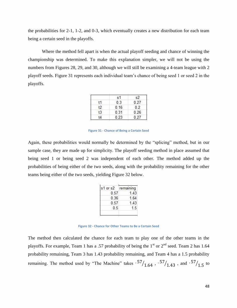
product within “The Machine” which projects statistics throughout the course of a season. The

team concluded that the contents of this project could be expanded upon and recommended how

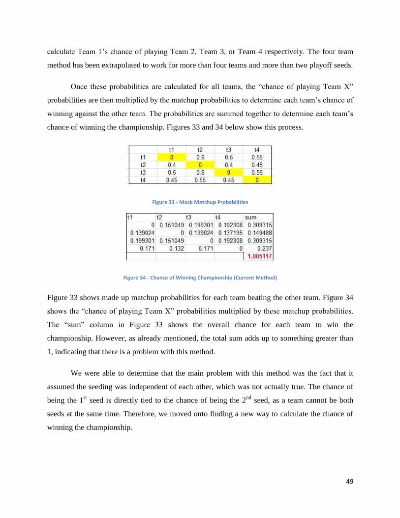
to do so consequently.

iii

Authorship

This report was developed through the collaborative efforts Mark Johnston, Ari Lathrop,

and Nicholas Mondor. All group members contributed equally to the completion of this project.

iv

Executive Summary

Advanced Sports Logic is an entrepreneurial company founded by WPI alumni Leonard

LaPadula that aims to provide its customers with a competitive advantage in fantasy football

leagues by increasing their overall chances of winning the league. Its software product, “The

Machine,” is designed to apply rigorous, mathematically sound formulas with the end goal of

providing recommendations on all possible player transactions available in fantasy football

leagues. With fantasy football becoming more and more popular amongst avid sports fans across

the world, Advanced Sports Logic has sought to further improve “The Machine” by asking our

group consisting of three senior actuarial mathematics majors from Worcester Polytechnic

Institute.

The project was broken down into three main objectives:

Generate different projection distributions for different tiers of players to account for

upside and downside potential.

Build and measure a method that uses historic data to generate projections which are both

accurate and detailed.

Review and refine the methods used to calculate playoff seeding and an individual team’s

chance of winning the championship.

For the first objective, the team gathered historical data from AccuScore (provided by

Advanced Sports Logic) and measured the overall accuracy and precision of the projection for

each player. We defined accuracy as a term to determine how accurate each of these projections

were, both in future weeks and the week right before the actual game; this was measured using

the . Meanwhile, we defined precision

(also known as variance throughout the report) as how much each projection changed throughout

the course of the season. Precision was found by taking the predictions in any given week and

calculating how much they change over the rest of the season (using standard deviation). In

addition, we generated a linear weighting scheme in an Excel file for the user so they could

choose which projections they valued the most throughout a season. By altering the three pivot

points found in Figure 16, the user was allowed to put a heavier weight on the predictions right

before the matchup, as well as lesser weights for weeks deeper into the future (or vice versa).

Additionally, we were also able to verify the “Shape shifting” method created by Advanced

Sports Logic, which determined player tiers for each position using total fantasy points scored.

v

The second objective of this project was broken down into four phases: (1) Defining what

data was needed; (2) Collecting the data; (3) Testing different methods for projections with the

data; and (4) Documenting results and creating recommendations.

The first thing that needed to be done for this objective was to determine all possible

factors for each position that should be taken into account when creating a projection model.

These factors can be found in section 3.2.1. After doing this, we then looked into a wide variety

of companies that kept historic football data. Eventually, we decided to have Advanced Sports

Logic purchase the data from TeamXML, which provided the data in a format that could be

extracted into an Excel file relatively easily. We then explored two different methods of

projecting statistics using a “top-down approach,” which involves predicting the statistics

(passing yards, rushing yards, receiving yards, touchdowns, interceptions, etc.) for each team for

an entire season and then allocating those stats to each game week-by-week. From there, the

approach looked to allocate the game-by-game statistics to individual players on each team.

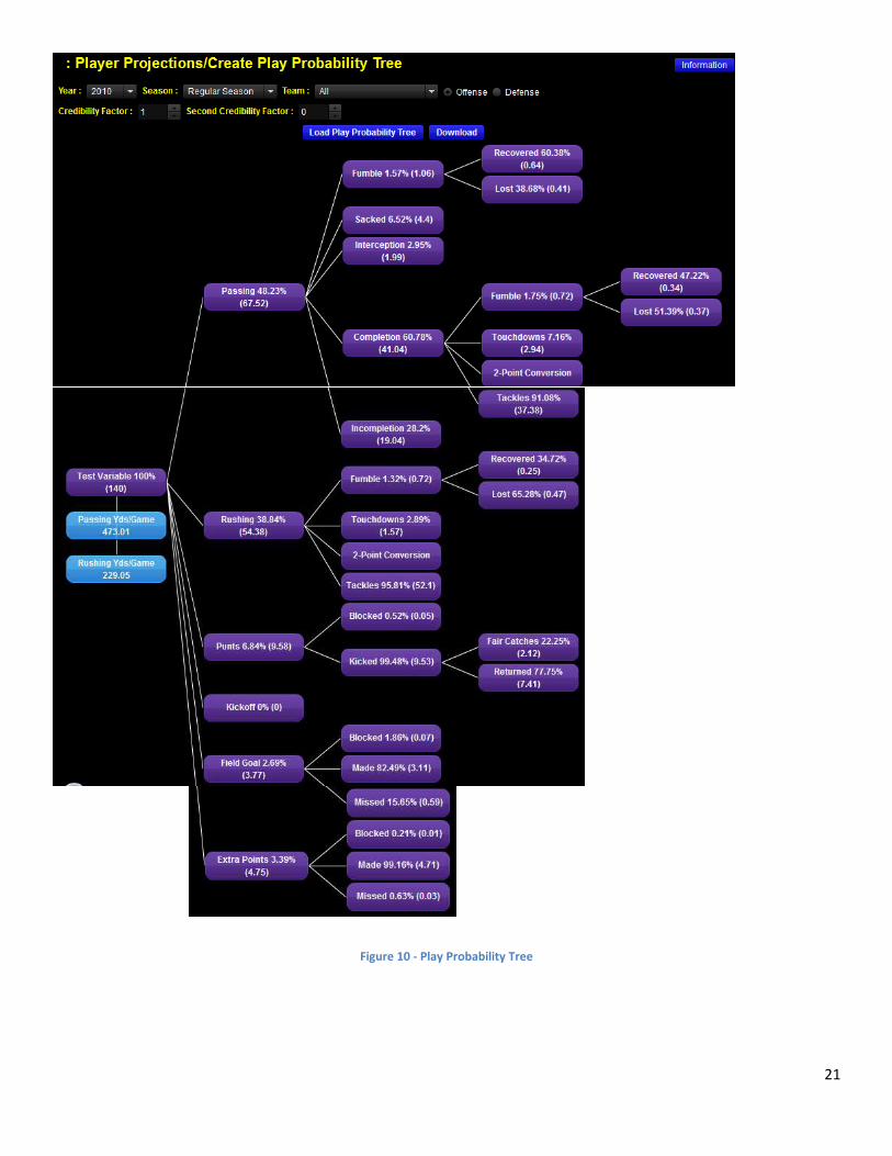
While exploring this “top-down approach,” the team decided to create a play probability

tree. We determined that there are a fixed number of things that can happen on any given play,

and those outcomes can happen with varying probabilities. From here, we were able to create

two different methods of projecting stats in conjunction with Advanced Sports Logic. The first

method involved blending the play probability trees together on a game-by-game basis and

creating a “predicted play probability tree.” This new probability tree was then multiplied by a

standard fantasy scoring rule set to yield team projections. The second method involved creating

an extremely basic Generalized Linear Model (GLM) using a variety of different parameters to

determine what would happen during each game.

We found that we were barely able to scratch the surface of the power of Generalized

Linear Models. However, our basic model yielded some interesting results, showing that a

method could be created to mathematically predict what would happen on a game-by-game

basis. Additionally, a direct comparison of the “predicted play probability tree” method to

AccuScore’s projections resulted in a graph showing that AccuScore overestimated their

projections in 2010 (Figure 23). The graph also showed that ASL’s basic projection method

vi

yielded a normal distribution, indicating that the projections at the team level were pretty

accurate.

The third objective involved exploring win probability methods and the various different

possibilities for playoff seeding in each league. We determined that the current method of

generating these seeding possibilities was not mathematically correct, and as such, explored

using conditional probability to solve the issue. However, the solution to the problem was much

simpler, as we already knew the playoff seeds by the time the playoffs came around. Therefore,

the only thing needed to determine a champion were the matchup probabilities as a team moved

throughout the playoffs.

While this project produced some very interesting results, the group still feels there is a

lot of work to be done. As such, we were able to come up with a number of different

recommendations:

1. Generate some sort of grading rubric for Objective 1 to determine what “good” accuracy

and precision numbers are.

2. Player tiers were created, but we recommend looking further into accounting for upside

and downside potential.

3. Investigate Generalized Linear Models further to determine the correlation between

variables, as they are a very powerful tool.

4. Determine a way to allocate team projections down to individual players. Doing so will

also help to determine whether or not the “top-down approach” is a valid projection

technique.

5. Look into conditional probability again for Objective 3, as the new method still feels too

simple to us.

vii

Table of Contents Abstract ......................................................................................................................................................... ii

Authorship ................................................................................................................................................... iii

Executive Summary ...................................................................................................................................... iv

1. Introduction ............................................................................................................................................. 1

2. Fantasy Sports and “The Machine” .......................................................................................................... 2

2.1 The History of Fantasy Sports ............................................................................................................. 2

2.2 Business Opportunities in Fantasy Sports ........................................................................................... 3

2.3 How Fantasy Football Works .............................................................................................................. 5

2.4 A Brief Explanation of “The Machine” ................................................................................................ 7

3. Improving “The Machine” ......................................................................................................................... 9

3.1 Objective 1: Building More Accurate Probability Distributions .......................................................... 9

3.1.1 Measuring Projection Accuracy and Precision ........................................................................... 11

3.1.2 Shape Shifting and Player Tiers .................................................................................................. 13

3.2 Objective 2: Creating a Method for Generating Fantasy Point Projections ..................................... 14

3.2.1 Phase 1: Data Definition ............................................................................................................ 14

3.2.2 Phase 2: Collecting the Data ...................................................................................................... 16

3.2.3 Phase 3: Testing Projection Methods ........................................................................................ 19

3.2.4 Phase 4: Documentation of Results ........................................................................................... 24

3.3 Objective 3: Reviewing and Refining Win Probability Methods ....................................................... 24

3.3.1 Analyzing the Current Playoff Seeding Method ......................................................................... 25

3.3.2 Creating a New Playoff Seeding Method ................................................................................... 28

3.3.3 Testing the Method .................................................................................................................... 29

4. Results from New Calculation Methods ................................................................................................. 30

4.1 Increased Accuracy on Probability Distribution Results ................................................................... 30

4.1.1 Accuracy and Precision .............................................................................................................. 30

4.1.2 Shape Shifting Results ............................................................................................................... 33

4.2 Projection Modeling Results ............................................................................................................. 38

4.2.1 Predicted Play Probability Tree Method .................................................................................... 38

4.2.2 Generalized Linear Model Results ............................................................................................. 40

4.3 Win Probability Results ..................................................................................................................... 44

4.3.1 Results of the Current Method .................................................................................................. 44

viii

4.3.2 Results from the New Win Probability Method ......................................................................... 50

5. Conclusions and Recommendations ....................................................................................................... 55

References .................................................................................................................................................. 58

Appendix A – Code for Win Probability Method ........................................................................................ 59

Appendix B – Excel Files .............................................................................................................................. 63

ix

Table of Figures

Figure 1 - FSTA Fantasy Sports Breakdown (CBS Sports, 2012) .................................................................... 3

Figure 2 - Statistics for Fantasy Football Players on CBSSports.com (CBS Sports, 2012) ............................. 4

Figure 3 - Flowchart of "The Machine" ......................................................................................................... 7

Figure 4 - Objective 1 Outline ..................................................................................................................... 10

Figure 5 - AccuScore Projection File ............................................................................................................ 11

Figure 6 - Linear Weighting Scheme ........................................................................................................... 13

Figure 7 - Phases for Projecting Fantasy Points .......................................................................................... 14

Figure 8 - TeamXML Query Builder (Page 1) ............................................................................................... 18

Figure 9 - TeamXML Query Builder (Page 2) ............................................................................................... 19

Figure 10 - Play Probability Tree ................................................................................................................. 21

Figure 11 - Objective 3 Methodology Flow Chart ....................................................................................... 25

Figure 12 - Example Win Probability Distribution ....................................................................................... 26

Figure 13 - Win/Loss Probability Distribution Graph .................................................................................. 28

Figure 14 - Proximity and Overall Accuracy Example ................................................................................. 30

Figure 15 - Precision Example ..................................................................................................................... 31

Figure 16 - Weighting Schematic ................................................................................................................ 32

Figure 17 - Weight Schematic Factored into Accuracy ............................................................................... 32

Figure 18 – Player Tiers Example ................................................................................................................ 35

Figure 19 - Tier 1 Running Backs ................................................................................................................. 36

Figure 20 - Tier 1 Defensive Backs .............................................................................................................. 36

Figure 21 - Tier 1 Wide Receivers ............................................................................................................... 37

Figure 22 - Objective 2 Ratio Sorting .......................................................................................................... 38

Figure 23 - Projection Comparison between ASL and AccuScore ............................................................... 39

Figure 24 - Generalized Linear Model for Pass TDs .................................................................................... 40

Figure 25 - Pass Predictions for Patriots in 2009 ........................................................................................ 41

Figure 26 - Patriots Predicted vs. Actual Graph .......................................................................................... 42

Figure 27 - Patriots Pass TD Delta Graph .................................................................................................... 43

Figure 28 - Mock Win Probabilities ............................................................................................................. 45

Figure 29 - Mock Win/Loss Probability Distribution ................................................................................... 46

Figure 30 - Stacked Win/Loss Probability Distribution ............................................................................... 47

Figure 31 - Chance of Being a Certain Seed ................................................................................................ 48

Figure 32 - Chance for Other Teams to Be a Certain Seed ......................................................................... 48

Figure 33 - Mock Matchup Probabilities ..................................................................................................... 49

Figure 34 - Chance of Winning Championship (Current Method) .............................................................. 49

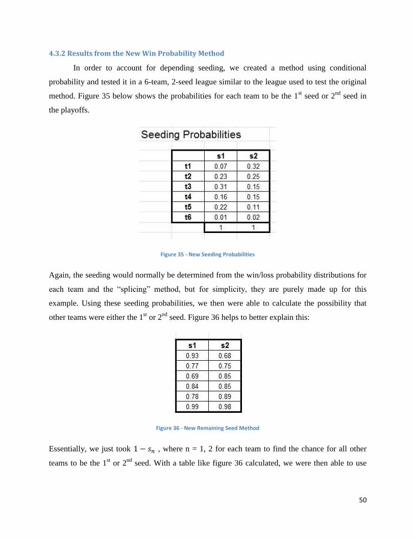
Figure 35 - New Seeding Probabilities ........................................................................................................ 50

Figure 36 - New Remaining Seed Method .................................................................................................. 50

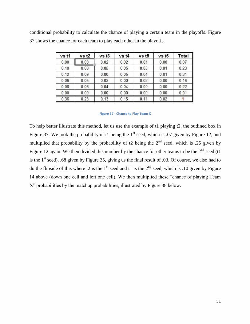
Figure 37 - Chance to Play Team X .............................................................................................................. 51

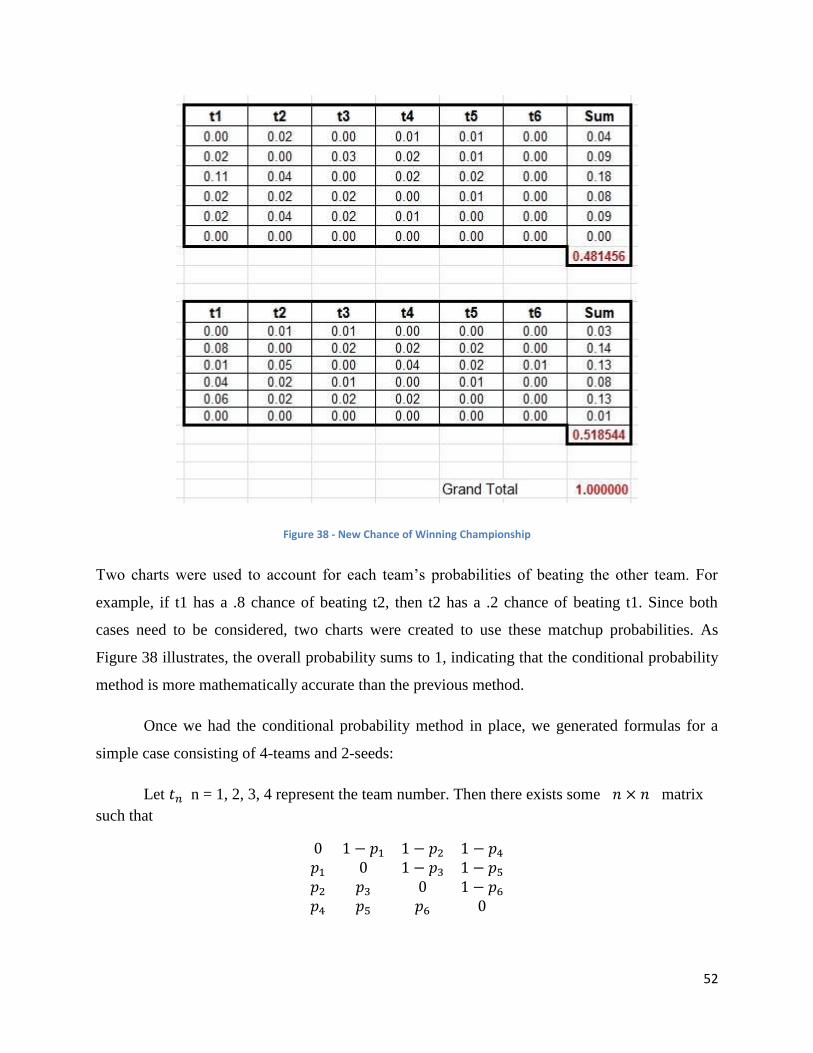
Figure 38 - New Chance of Winning Championship ................................................................................... 52

1

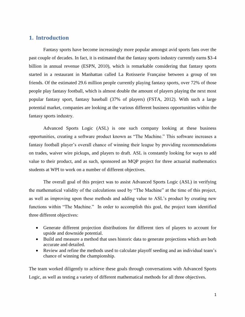
1. Introduction

Fantasy sports have become increasingly more popular amongst avid sports fans over the

past couple of decades. In fact, it is estimated that the fantasy sports industry currently earns $3-4

billion in annual revenue (ESPN, 2010), which is remarkable considering that fantasy sports

started in a restaurant in Manhattan called La Rotisserie Française between a group of ten

friends. Of the estimated 29.6 million people currently playing fantasy sports, over 72% of those

people play fantasy football, which is almost double the amount of players playing the next most

popular fantasy sport, fantasy baseball (37% of players) (FSTA, 2012). With such a large

potential market, companies are looking at the various different business opportunities within the

fantasy sports industry.

Advanced Sports Logic (ASL) is one such company looking at these business

opportunities, creating a software product known as “The Machine.” This software increases a

fantasy football player’s overall chance of winning their league by providing recommendations

on trades, waiver wire pickups, and players to draft. ASL is constantly looking for ways to add

value to their product, and as such, sponsored an MQP project for three actuarial mathematics

students at WPI to work on a number of different objectives.

The overall goal of this project was to assist Advanced Sports Logic (ASL) in verifying

the mathematical validity of the calculations used by “The Machine” at the time of this project,

as well as improving upon these methods and adding value to ASL’s product by creating new

functions within “The Machine.” In order to accomplish this goal, the project team identified

three different objectives:







The team worked diligently to achieve these goals through conversations with Advanced Sports

Logic, as well as testing a variety of different mathematical methods for all three objectives.

2

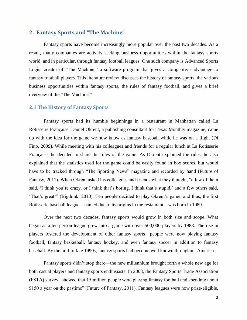
2. Fantasy Sports and “The Machine”

Fantasy sports have become increasingly more popular over the past two decades. As a

result, many companies are actively seeking business opportunities within the fantasy sports

world, and in particular, through fantasy football leagues. One such company is Advanced Sports

Logic, creator of “The Machine,” a software program that gives a competitive advantage to

fantasy football players. This literature review discusses the history of fantasy sports, the various

business opportunities within fantasy sports, the rules of fantasy football, and gives a brief

overview of the “The Machine.”

2.1 The History of Fantasy Sports

Fantasy sports had its humble beginnings in a restaurant in Manhattan called La

Rotisserie Française. Daniel Okrent, a publishing consultant for Texas Monthly magazine, came

up with the idea for the game we now know as fantasy baseball while he was on a flight (Di

Fino, 2009). While meeting with his colleagues and friends for a regular lunch at La Rotisserie

Française, he decided to share the rules of the game. As Okrent explained the rules, he also

explained that the statistics used for the game could be easily found in box scores, but would

have to be tracked through “The Sporting News” magazine and recorded by hand (Future of

Fantasy, 2011). When Okrent asked his colleagues and friends what they thought, “a few of them

said, ‘I think you’re crazy, or I think that’s boring, I think that’s stupid,’ and a few others said,

‘That’s great’” (Bigthink, 2010). Ten people decided to play Okrent’s game, and thus, the first

Rotisserie baseball league—named due to its origins in the restaurant—was born in 1980.

Over the next two decades, fantasy sports would grow in both size and scope. What

began as a ten person league grew into a game with over 500,000 players by 1988. The rise in

players fostered the development of other fantasy sports—people were now playing fantasy

football, fantasy basketball, fantasy hockey, and even fantasy soccer in addition to fantasy

baseball. By the mid-to-late 1990s, fantasy sports had become well known throughout America.

Fantasy sports didn’t stop there—the new millennium brought forth a whole new age for

both casual players and fantasy sports enthusiasts. In 2003, the Fantasy Sports Trade Association

(FSTA) survey “showed that 15 million people were playing fantasy football and spending about

$150 a year on the pastime” (Future of Fantasy, 2011). Fantasy leagues were now prize-eligible,

3

pay-to-play leagues, meaning that for a small entrance fee, players had the ability to participate

in leagues where the winner would receive a cash prize. Additionally, the high level of interest

resulted in television shows, blogs, and other means of media strictly dedicated to fantasy sports.

As of January 16th

, 2012, it is estimated that there are approximately 29.6 million fantasy

sports players in the United States alone (Fantasy Sports Trade Association, 2012). According to

a fantasy sports quiz issued by the Entertainment and Sports Programming Network (ESPN), it is

also estimated that fantasy sports produces $3-4 billion in annual revenue (ESPN, 2010).

2.2 Business Opportunities in Fantasy Sports

With approximately 29.6 million fantasy sports players and a 3-4 billion dollar industry,

it is no secret that there are many potential business opportunities within fantasy sports. CBS

Sports’ publication The Next Generation of Fantasy Sports: The Open Fantasy Platform at

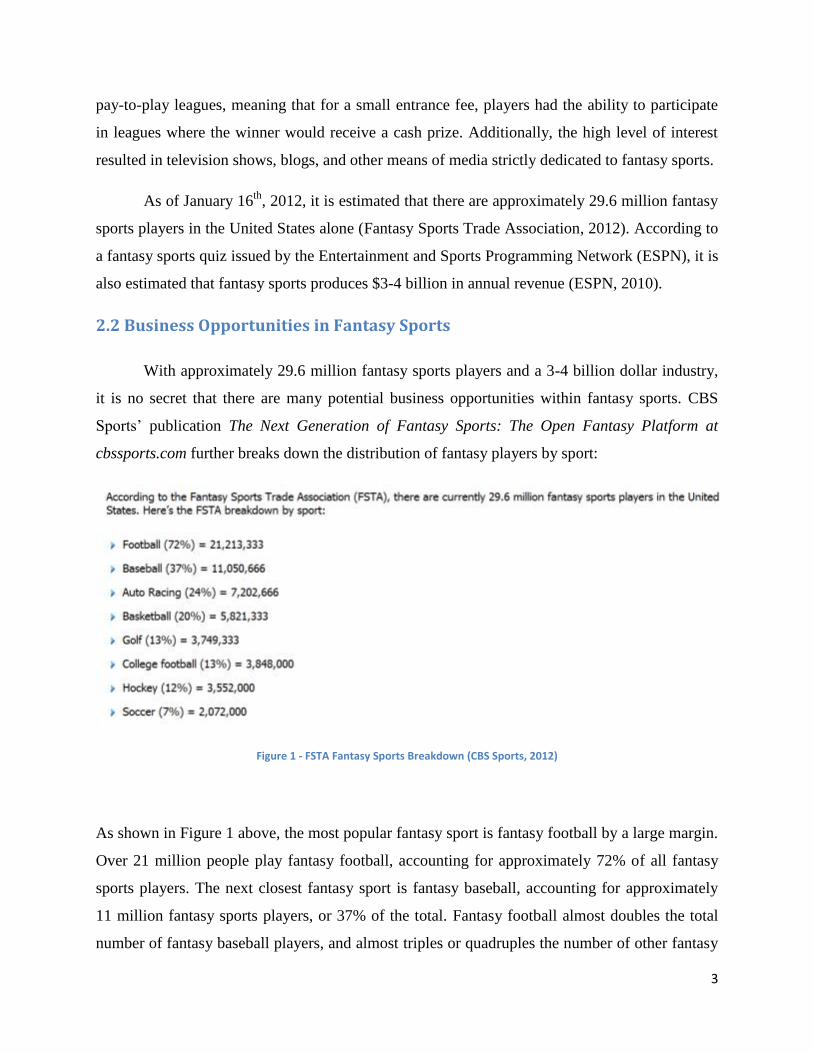
cbssports.com further breaks down the distribution of fantasy players by sport:

Figure 1 - FSTA Fantasy Sports Breakdown (CBS Sports, 2012)

As shown in Figure 1 above, the most popular fantasy sport is fantasy football by a large margin.

Over 21 million people play fantasy football, accounting for approximately 72% of all fantasy

sports players. The next closest fantasy sport is fantasy baseball, accounting for approximately

11 million fantasy sports players, or 37% of the total. Fantasy football almost doubles the total

number of fantasy baseball players, and almost triples or quadruples the number of other fantasy

4

sports players participating in fantasy auto racing, fantasy basketball, and fantasy golf. However,

it is important to note that the data provided by the FSTA includes players who may play

multiple fantasy sports. In other words, the data shows the number of non-unique players in each

fantasy sport.

The same CBS publication provides valuable insight into the potential market for

Advanced Sports Logic, which already gives CBS Sports’ fantasy football players the option of

buying their team selection software known as “The Machine.” According to the Nielsen Net

Ratings for fantasy sports, “fantasy football players on CBSSports.com register the highest level

of engagement of any major site, with players spending an average of 1 hour, 41 minutes per

session and returning 4 times each week to research and optimize their rosters” (CBS Sports,

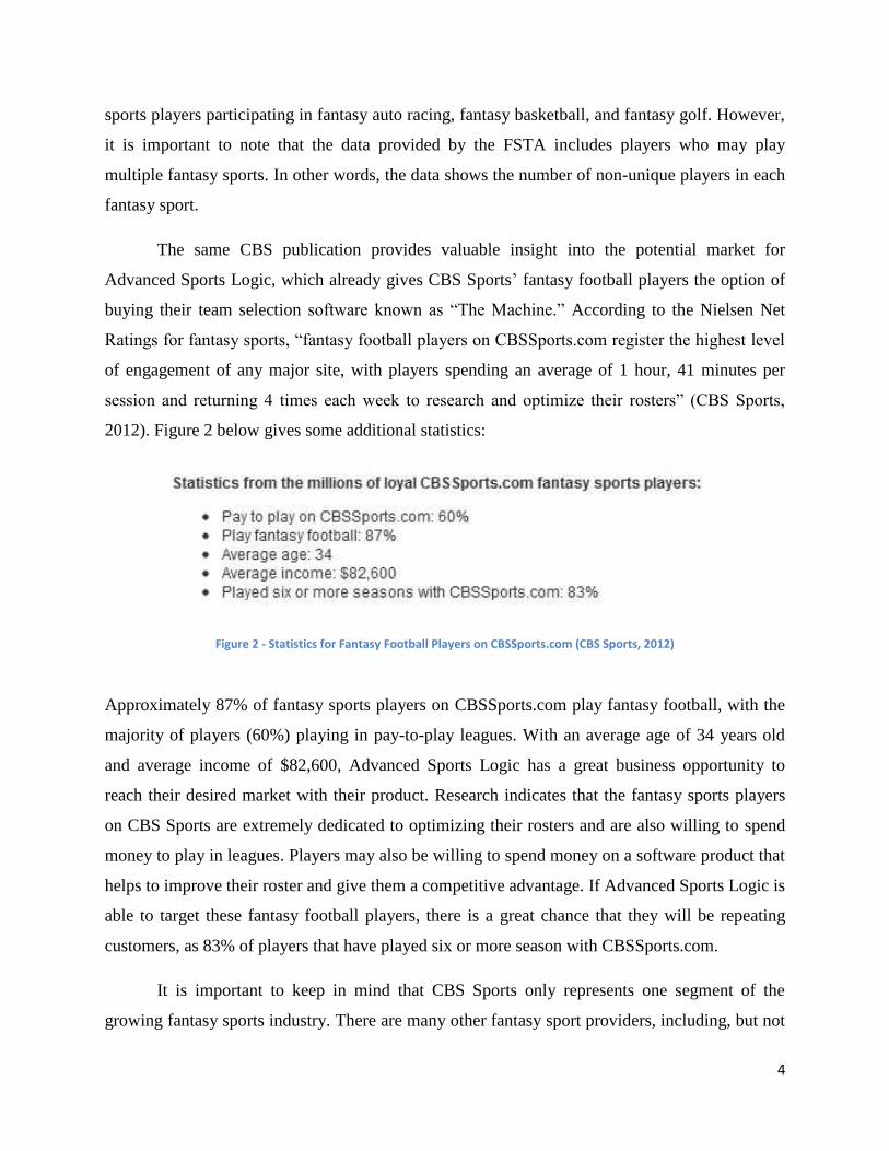
2012). Figure 2 below gives some additional statistics:

Figure 2 - Statistics for Fantasy Football Players on CBSSports.com (CBS Sports, 2012)

Approximately 87% of fantasy sports players on CBSSports.com play fantasy football, with the

majority of players (60%) playing in pay-to-play leagues. With an average age of 34 years old

and average income of $82,600, Advanced Sports Logic has a great business opportunity to

reach their desired market with their product. Research indicates that the fantasy sports players

on CBS Sports are extremely dedicated to optimizing their rosters and are also willing to spend

money to play in leagues. Players may also be willing to spend money on a software product that

helps to improve their roster and give them a competitive advantage. If Advanced Sports Logic is

able to target these fantasy football players, there is a great chance that they will be repeating

customers, as 83% of players that have played six or more season with CBSSports.com.

It is important to keep in mind that CBS Sports only represents one segment of the

growing fantasy sports industry. There are many other fantasy sport providers, including, but not

5

limited to: ESPN, Yahoo!, Fox, Fantasy Sharks, etc. Expanding the company and offering “The

Machine” to players on other websites will allow for an even greater business opportunity for

Advanced Sports Logic.

2.3 How Fantasy Football Works

Before we take a closer look at “The Machine,” we must first have a basic understanding

of how fantasy football works. While there are a variety of different categories and sets of rules,

the overall objective of the game is always the same—score more fantasy points than your

opponent.

The very first aspect of fantasy football involves signing up or creating a league. There

are many different options available for fantasy football players—they can sign up for free

leagues as well as prize-eligible leagues. Prize-eligible leagues require an entrance fee for each

participant—the winner of the league receives a larger sum of money after commissions are

taken out. The size of a league can range from two to twenty players; the standard size for a

league on CBS Sports is twelve players. Additionally, leagues can either be public or private,

meaning that they can be open to the public or require a password to join, respectively.

The next aspect of fantasy football involves a league-wide draft in which each team

selects their players. There are two types of drafts: (1) Snake and (2) Auction. Snake drafts

arrange the picks like a snake, with the first overall pick having the last pick in the 2nd

round and

1st pick in the 3

rd round, second overall pick having the second to last pick in the 2

nd round and

2nd

pick in the 3rd

round, etc. Auction drafts allow fantasy players to essentially “win” players

depending on how much money is put down on a certain player. Players may outbid each other

to acquire a certain player, but need to manage their money carefully as there is a spending limit.

Drafts conclude when a team fills its roster with starters and bench players. In CBS

Sports standard leagues, a full team means 1 Quarterback, 2 Running Backs, 2 Wide Receivers, 1

“Flex” (either Running Back or Wide Receiver), 1 Tight End, 1 Kicker, 1 Defense/Special

Teams, and 6 Bench players. Bench players may be moved from “Reserve” status to “Active” in

any given week, but rosters lock before the games begin to ensure players cannot make changes

as games are in progress.

6

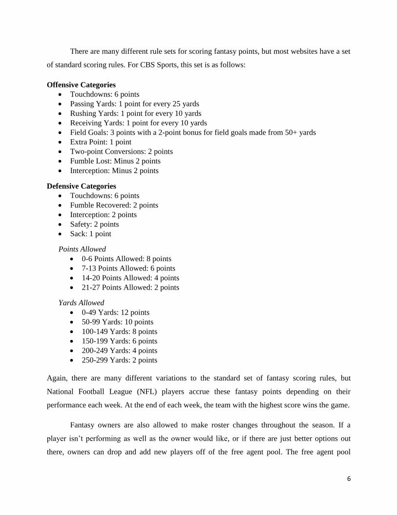
There are many different rule sets for scoring fantasy points, but most websites have a set

of standard scoring rules. For CBS Sports, this set is as follows:

Offensive Categories

Touchdowns: 6 points

Passing Yards: 1 point for every 25 yards

Rushing Yards: 1 point for every 10 yards

Receiving Yards: 1 point for every 10 yards

Field Goals: 3 points with a 2-point bonus for field goals made from 50+ yards

Extra Point: 1 point

Two-point Conversions: 2 points

Fumble Lost: Minus 2 points

Interception: Minus 2 points

Defensive Categories

Touchdowns: 6 points

Fumble Recovered: 2 points

Interception: 2 points

Safety: 2 points

Sack: 1 point

Points Allowed

0-6 Points Allowed: 8 points




Yards Allowed

0-49 Yards: 12 points






Again, there are many different variations to the standard set of fantasy scoring rules, but

National Football League (NFL) players accrue these fantasy points depending on their

performance each week. At the end of each week, the team with the highest score wins the game.

Fantasy owners are also allowed to make roster changes throughout the season. If a

player isn’t performing as well as the owner would like, or if there are just better options out

there, owners can drop and add new players off of the free agent pool. The free agent pool

7

contains all players who weren’t drafted at the start of the season and have not been acquired by

another owner in the league. Additionally, owners can also make trades depending on their

team’s needs.

2.4 A Brief Explanation of “The Machine”

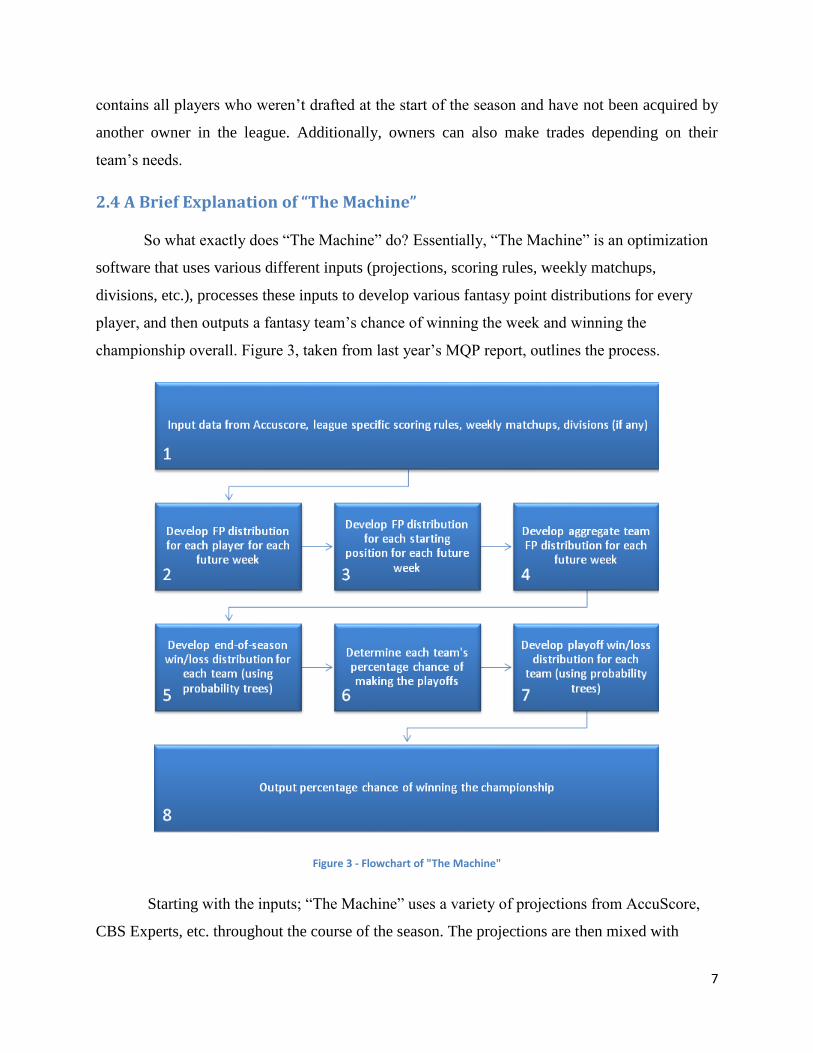
So what exactly does “The Machine” do? Essentially, “The Machine” is an optimization

software that uses various different inputs (projections, scoring rules, weekly matchups,

divisions, etc.), processes these inputs to develop various fantasy point distributions for every

player, and then outputs a fantasy team’s chance of winning the week and winning the

championship overall. Figure 3, taken from last year’s MQP report, outlines the process.

Figure 3 - Flowchart of "The Machine"

Starting with the inputs; “The Machine” uses a variety of projections from AccuScore,

CBS Experts, etc. throughout the course of the season. The projections are then mixed with

8

league specific variables such as scoring rules, weekly matchups, and divisions. “The Machine”

uses the information to calculate fantasy point distributions for each player for every week in the

season, the next step in the process outlined by Figure 3.

Now, these fantasy point distributions created from the inputs change as the projections

for each player change. For example, if a player was predicted to score 18 points in Week 1, but

only scored 12 points, it is possible that the projections would change to account for that player

not being as productive as originally thought. The change in projections is reflected in the

fantasy point distribution for that player for every future week, not just Week 2.

Using the information explained above, “The Machine” is able to build fantasy point

distributions for an entire team and calculate a team’s chance of beating another team based on

these aggregate team distributions. Additionally, “The Machine” also recommends free agent

pickups and trades that can help improve a player’s team, hence increasing their overall chances

of winning their matchups each week.

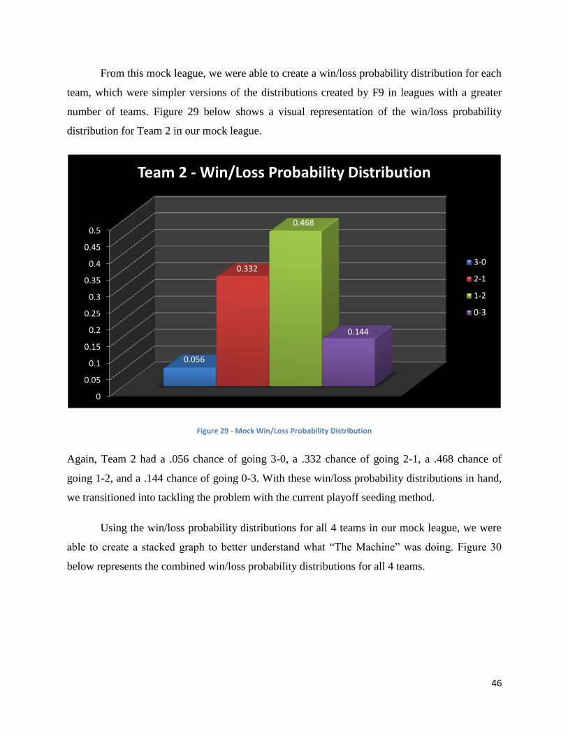
The final output of “The Machine” is the overall chance of winning the championship.

Using the aggregate team distributions, the software is able to create win/loss probability

distributions, meaning that it creates a graph with a fantasy team’s chance of going 0-12, 1-11, 2-

10, 3-9, 4-8, 5-7, etc. From this, it is able to determine a team’s playoff seed and the overall

chance of winning the championship. However, there have been changes to that system, which

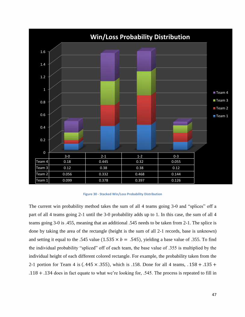
are later discussed in sections 3.3, 4.3, and 5.

9

3. Improving “The Machine”

The overall goal of this project was to assist Advanced Sports Logic (ASL) in verifying

the mathematical validity of the calculations used by “The Machine” at the time of this project,

as well as improving upon these methods and adding value to ASL’s product by creating new

functions within “The Machine.” In order to accomplish this goal, the project team identified

three different objectives:







In order to accomplish these objectives, the project team used a variety of data collection,

calculation, and testing methods. Some of these methods included meeting with ASL’s CEO to

gather information on how “The Machine” currently does its calculations, purchasing and

reorganizing historical football data into a more usable format, creating several different

mathematical prediction models and statistical weighting schemes, and testing prediction models

and weighting schemes using the purchased historical data.

3.1 Objective 1: Building More Accurate Probability Distributions

One of the main improvements that the project team focused on was modifying the player

probability distributions generated by “The Machine.” As outlined in section 2.4, these are the

probability distributions created using projections, as well as league specific inputs such as

scoring rules. “The Machine” does not currently account for different tiers of players; players

that are projected at high performance levels typically have more downside potential than upside

potential, whereas players projected at low performance levels typically have more upside

potential than downside potential.

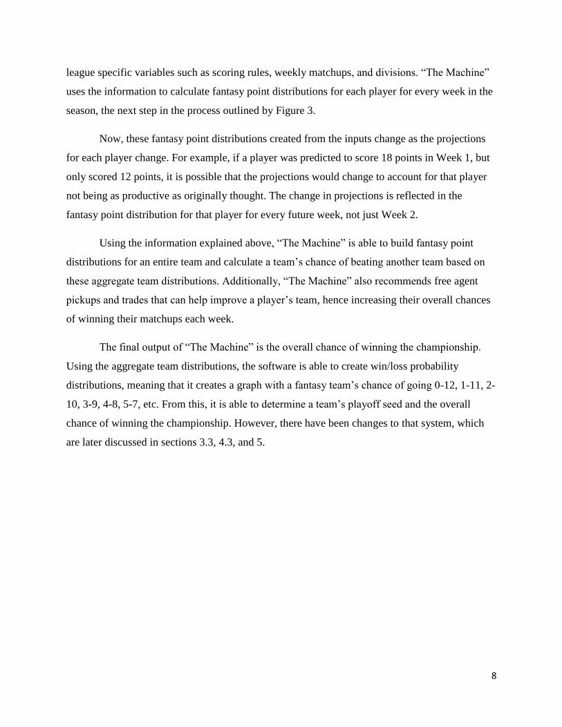
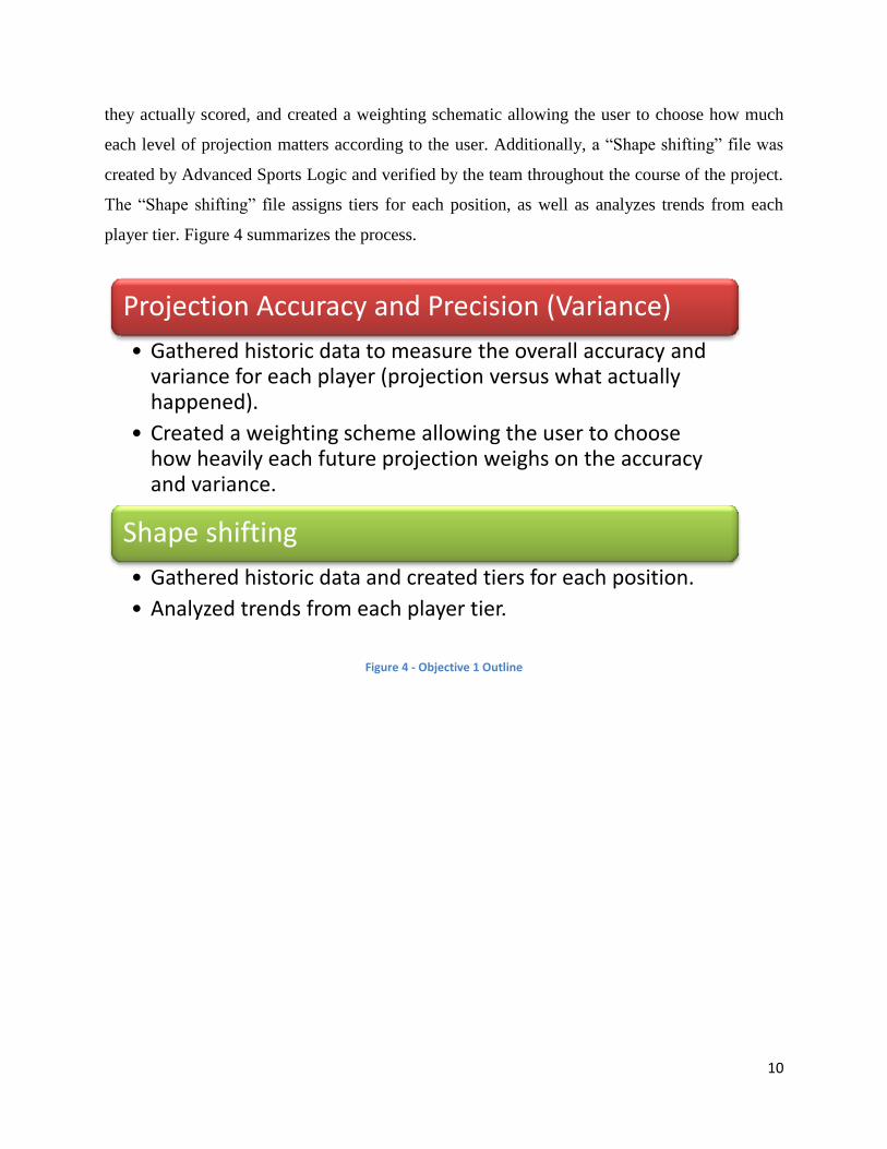
To account for this upside and downside potential, we gathered historical data from

AccuScore, measured the accuracy and standard deviation of each player projection versus what

10

they actually scored, and created a weighting schematic allowing the user to choose how much

each level of projection matters according to the user. Additionally, a “Shape shifting” file was

created by Advanced Sports Logic and verified by the team throughout the course of the project.

The “Shape shifting” file assigns tiers for each position, as well as analyzes trends from each

player tier. Figure 4 summarizes the process.

Figure 4 - Objective 1 Outline

Projection Accuracy and Precision (Variance)

• Gathered historic data to measure the overall accuracy and variance for each player (projection versus what actually happened).

• Created a weighting scheme allowing the user to choose how heavily each future projection weighs on the accuracy and variance.

Shape shifting

• Gathered historic data and created tiers for each position.

• Analyzed trends from each player tier.

11

3.1.1 Measuring Projection Accuracy and Precision

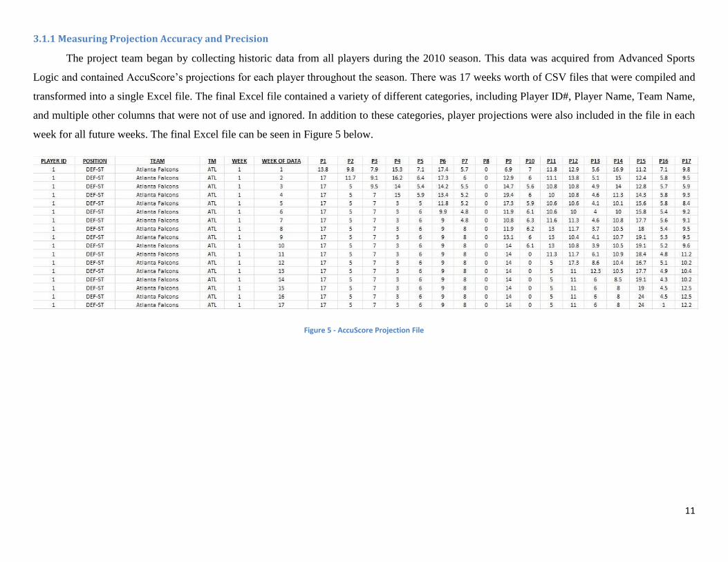
The project team began by collecting historic data from all players during the 2010 season. This data was acquired from Advanced Sports

Logic and contained AccuScore’s projections for each player throughout the season. There was 17 weeks worth of CSV files that were compiled and

transformed into a single Excel file. The final Excel file contained a variety of different categories, including Player ID#, Player Name, Team Name,

and multiple other columns that were not of use and ignored. In addition to these categories, player projections were also included in the file in each

week for all future weeks. The final Excel file can be seen in Figure 5 below.

Figure 5 - AccuScore Projection File

12

The “Week of Data” column indicates which week the data came from, whereas P1, P2, … , P17

indicate the projections for each future week going across the cells. Taking a quick look at P1,

you will notice that there the value is “17” for “Week of Data” 2-17. This number represents

what the player—in this case the Atlanta Falcons DEF-ST—actually scored in Week 1.

However, you’ll also notice that the projections in “Week of Data” 2 change going across the

row. For example, P2 changed from 9.8 to 11.7, P3 changed from 7.9 to 9.1, P4 changed from

15.3 to 16.2, etc.

After the data was compiled, we made sure to eliminate all players without 17 full weeks

of data. This was due to a complication with the formulas to calculate accuracy and precision

more than anything, but also due to the fact that we wanted complete data sets for all players we

were analyzing.

From the Excel file shown in figure 5, we were able to generate accuracy and precision,

which is further explained in section 4.1.1. Accuracy was measured by taking

, whereas precision was calculated by taking the standard deviation of the

predictions going down each column (P2, P3, P4, etc.). The precision aimed to quantify how

much each projection changed throughout the course of the season, while accuracy aimed to

quantify how accurate each of these projections were, both in future weeks and the week right

before the actual game.

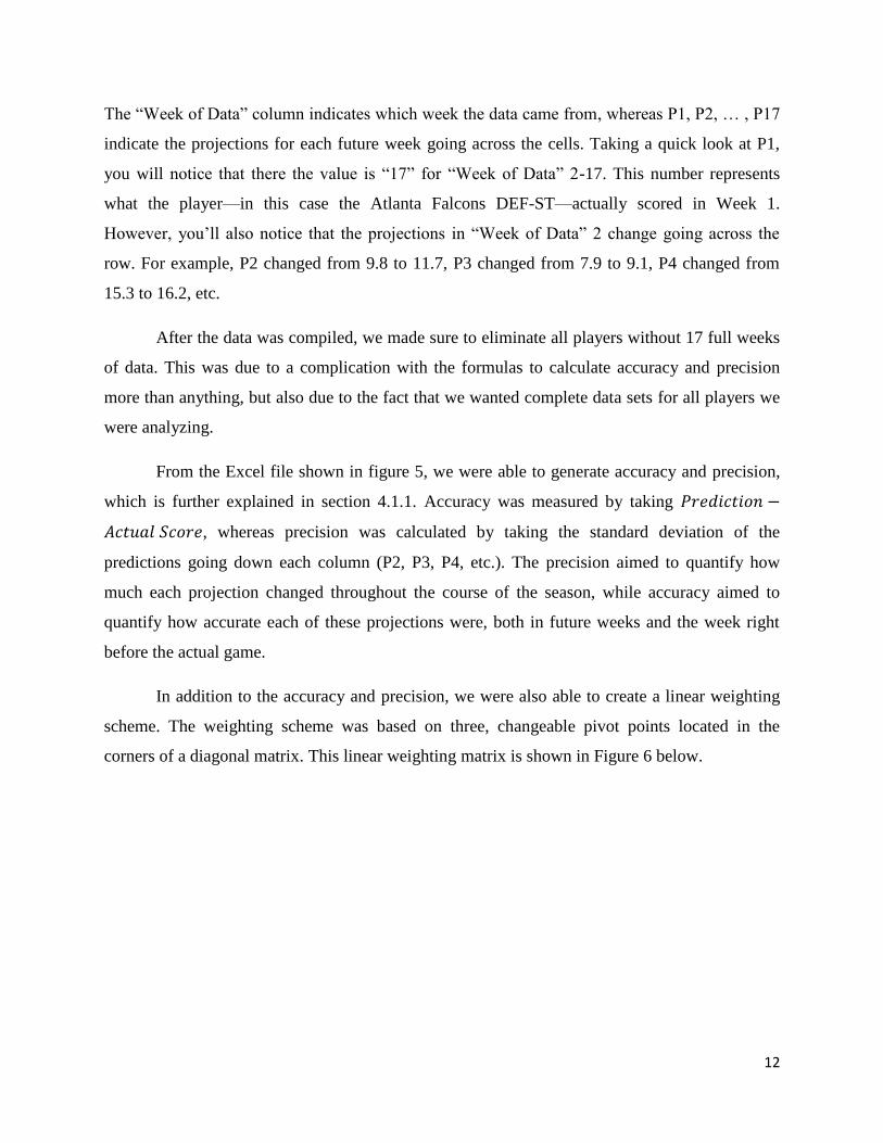
In addition to the accuracy and precision, we were also able to create a linear weighting

scheme. The weighting scheme was based on three, changeable pivot points located in the

corners of a diagonal matrix. This linear weighting matrix is shown in Figure 6 below.

13

Figure 6 - Linear Weighting Scheme

While we allowed negative numbers on the pivot points to put weighting emphasis on a variety

of different places, if the weight is negative anywhere aside from these pivot points, it is

automatically set to 0. The user is able to put a heavier weight on the predictions right before the

matchup rather than in future weeks without having negative weights in these future weeks. Of

course, the opposite can also be done depending on where the user wants the most emphasis.

3.1.2 Shape Shifting and Player Tiers

The “Shape shifting” method used a similar Excel file composed of past historical data

from AccuScore to generate different tiers of players. These tiers were created using the overall

amount of fantasy points scored in a single season. Tiers were organized as follows:

1. 1-10 ranked players



4. All players that do not have all 0 for fantasy points

5. All players with all 0’s for fantasy points

Additionally, the accuracy and precision of the predictions were also calculated in the “Shape

shifting” method, but in a different manner. The accuracy only took into account the last

prediction (i.e. the prediction right before the game actually happens) and the precision only took

into account how much the predictions vary prior to the start of the season rather than throughout

the entire season. This data was further used in Objective 2 to see how accurate AccuScore’s

projections were versus the ASL projection model.

14

3.2 Objective 2: Creating a Method for Generating Fantasy Point Projections

There are many different companies that currently generate fantasy football point

projections including, but not limited to: AccuScore, CBS Sports, ESPN, and Fantasy Sharks. To

add value to “The Machine,” Advanced Sports Logic aims to be able to generate their own set of

projections more accurate than those generated by the companies listed above. Since AccuScore

is the only company (to our knowledge) that projects how players will do in all future weeks on a

week to week basis, Advanced Sports Logic has an opportunity to capture a part of the

projections market and set themselves apart from the competition.

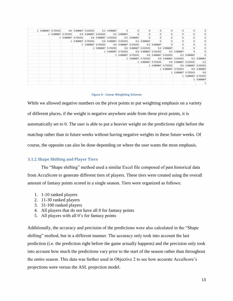
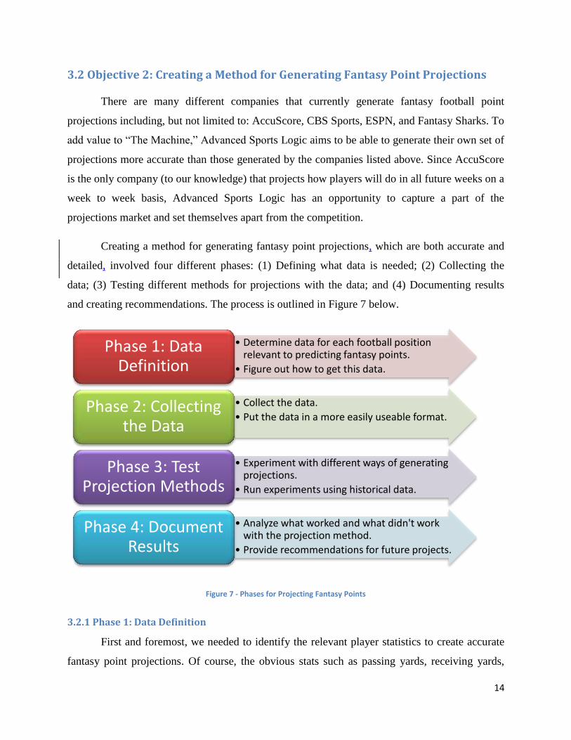
Creating a method for generating fantasy point projections, which are both accurate and

detailed, involved four different phases: (1) Defining what data is needed; (2) Collecting the

data; (3) Testing different methods for projections with the data; and (4) Documenting results

and creating recommendations. The process is outlined in Figure 7 below.

Figure 7 - Phases for Projecting Fantasy Points

3.2.1 Phase 1: Data Definition

First and foremost, we needed to identify the relevant player statistics to create accurate

fantasy point projections. Of course, the obvious stats such as passing yards, receiving yards,

• Determine data for each football position relevant to predicting fantasy points.

• Figure out how to get this data.

Phase 1: Data Definition

• Collect the data.

• Put the data in a more easily useable format. Phase 2: Collecting

the Data

• Experiment with different ways of generating projections.

• Run experiments using historical data.

Phase 3: Test Projection Methods

• Analyze what worked and what didn't work with the projection method.

• Provide recommendations for future projects.

Phase 4: Document Results

15

rushing yards, touchdowns, sacks, interceptions, points allowed, field goals, extra points, etc. are

needed to be able to project fantasy points on a week to week basis. However, there are many

additional factors that could be considered in a projection model. We decided to break down

these factors by position:

Quarterback

Offensive Line

Opposing defensive pass rush

Cornerbacks

Offensive receivers (talent)

Backs ability to block

Yards out of pocket vs. yards in the pocket

Arm strength/ability to fit the ball into tight windows

Wide Receiver

Cornerbacks

o Going along with this, receiver and cornerback size might come into play. Is the

receiver able to make catches over the cornerback? Quality of the cornerback

guarding the receiver is also something to make note of; for example defenders

such as Darrelle Revis don’t let the receiver they are guarding catch many balls.

Quarterback (talent)

Running Back

Offensive line

Defense , mostly defensive line

Fullback blocking

Downfield blocking

o Receivers blocking

Maybe measure how many runs went to the left, through the middle, and to the right

(outside speed running vs. power running)

Carries inside the 5 yard line (different RBs get carries as you get closer to the goal

line—Brandon Jacobs, Michael Bush, just to name a few)

Tight End

Quarterback (talent)

Defense

Blocks by RB

Size (Most TEs are larger in size due to the nature of the position and those that are good

route runners and have good hands can create mismatches against smaller defenders)

Kicker

Ability to score touchdowns

o 3rd

down conversion percentage could come into play into these two categories

16

Ability to move down the field

o Average starting yard line per drive and average yards earned per drive could

indicate how likely a kicker is to kick field goals vs. touchdowns

Leg strength vs. accuracy

o Look at percentage of kicks made from 10-20 yards, 20-30 yards, 30-40 yards, etc

D/ST

Opposing special teams/offense

Good kick/punt returner

Good kicker/punter

In addition to these positional factors, we also identified some additional parameters that did not

necessarily fit under these positions, such as:

Home vs. Away

Indoor vs. Outdoor

Weather

Altitude (for example Denver)

Player Age and Injury Record

While coming up with these factors was a relatively easy process, we initially struggled to

understand how all of these factors were going to be used to come up with a projection model.

We also had no idea if these factors would be quantifiable, and even if they were quantifiable,

we were unsure if these factors would be readily available to either find or purchase from another

company.

3.2.2 Phase 2: Collecting the Data

All of the necessary data (i.e. passing yards, rushing yards, receiving yards, touchdowns,

sacks, interceptions, etc.) was readily available on sites such as ESPN and Yahoo, but gathering

this data and pulling it from the websites into a central location would have been extremely

tedious. Additionally, most of the positional factors that we identified in section 3.2.1 were not

readily available even from companies that keep track of statistical data.

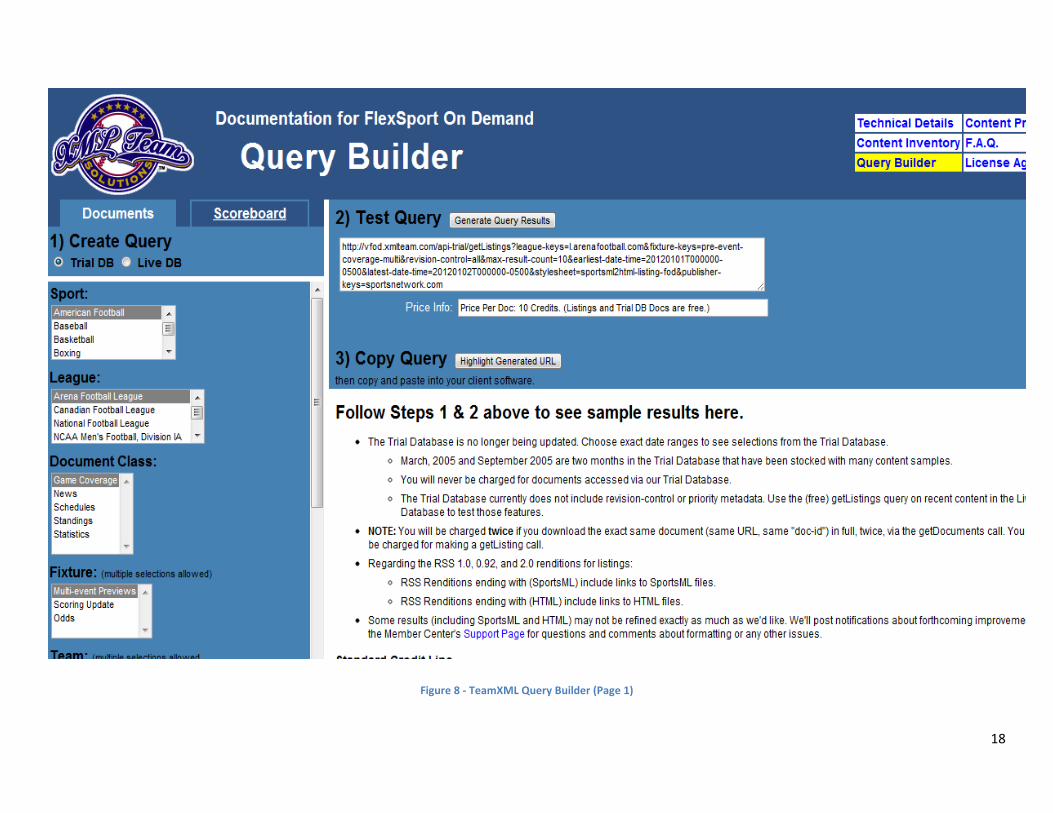
With these issues in mind, we looked to outsource the data gathering process. The team

took a look at quite a few companies that kept track of historical football data, but we eventually

decided to purchase from a company called TeamXML. TeamXML had the data in a format that

could be easily manipulated to fit our needs. As such, 5 years of data was purchased, consisting

17

of the basics needed to come up with a projection model (i.e. passing yards, rushing yards,

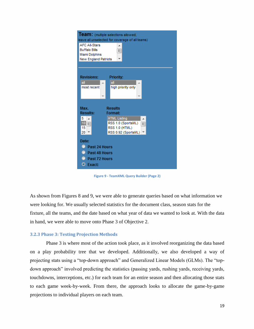
receiving yards, touchdowns, sacks, interceptions, etc.). Figures 8 and 9 below show what the

TeamXML website (http://fod.xmlteam.com/documentation/query-builder/) looked like after the

data was purchased.

http://fod.xmlteam.com/documentation/query-builder/

18

Figure 8 - TeamXML Query Builder (Page 1)

19

Figure 9 - TeamXML Query Builder (Page 2)

As shown from Figures 8 and 9, we were able to generate queries based on what information we

were looking for. We usually selected statistics for the document class, season stats for the

fixture, all the teams, and the date based on what year of data we wanted to look at. With the data

in hand, we were able to move onto Phase 3 of Objective 2.

3.2.3 Phase 3: Testing Projection Methods

Phase 3 is where most of the action took place, as it involved reorganizing the data based

on a play probability tree that we developed. Additionally, we also developed a way of

projecting stats using a “top-down approach” and Generalized Linear Models (GLMs). The “top-

down approach” involved predicting the statistics (passing yards, rushing yards, receiving yards,

touchdowns, interceptions, etc.) for each team for an entire season and then allocating those stats

to each game week-by-week. From there, the approach looks to allocate the game-by-game

projections to individual players on each team.

20

With the “top-down approach” in mind, we were able to develop what we refer to as the

play probability tree. The tree accounted for all possible outcomes for a single play. For example,

a play could end up in a pass, a run, or a kick. From there, if the play is a pass, there are multiple

different things that could happen, such as the quarterback fumbling the ball before the pass,

getting sacked by the defense, throwing an interception, throwing an incompletion, throwing a

completion for a certain number of yards, or throwing a completion for a touchdown. Similar

situations were developed for running and kicking plays, outlined in Figure 10 below.

21

Figure 10 - Play Probability Tree

22

The play probability tree was coded into the Projection Developer page on Advanced Sports

Logic’s website (http://asl-qa.com/ff2011/). The play probability tree can be generated for either

the whole NFL or a specific team for the preseason, regular season, and playoffs. In addition the

user can enter in a credibility factor, the highest being 1 and the lowest being 0, for the tree. This

credibility factor is essentially a weighting schematic that allows the user to select how much

weight should be placed on more recent weeks for projection purposes, which will be explained

later in this section. The larger the credibility factor, the more weight is placed on recent weeks.

Figure 10 also shows that each branch of the tree has been populated with a certain

percentage. These percentages were generated from the historic data purchased from TeamXML

and formatted into a specific manner. The data populating each tree can be easily downloaded as

a CSV file, allowing the user to see the raw statistics rather than just the percentages in the tree.

With the sorted data in place, it was time to come up with a method of projecting

statistics using our “top-down approach.” Advanced Sports Logic came up with a method using

the play probability tree, whereas the project team came up with a second method using

Generalized Linear Models.

The play probability tree projection method blended together two play probability trees

(one for both the defense and offense for each team) to generate a “predicted” play probability

tree for a game. The credibility factor was also used to determine how much data these play

probability trees should take into account. The default was set to 1 after testing what value

should be used, as a credibility factor of 1 yielded the most accurate projections when compared

to what actually happened in 2010.

Once these “predicted” play probability trees for a game were created, the total amount of

predicted fantasy points were generated by multiplying the percentages of the tree by a standard

fantasy football scoring rule set. Additionally, the sum of individual player projections by

AccuScore for each team on a game-by-game basis yielded “team” projections from a “bottom-

up approach.” Each game had two projections in each set (two for the predicted play probability

tree and two for the “bottom-up approach”), one overall projection for each team. The overall

projections were then compared to what actually happened and put into bins depending on how

far off the overall projections were from the actual fantasy points scored. A scale from -100% to

http://asl-qa.com/ff2011/

23

100% with bin values in between was used to create a comparison between ASL’s projection

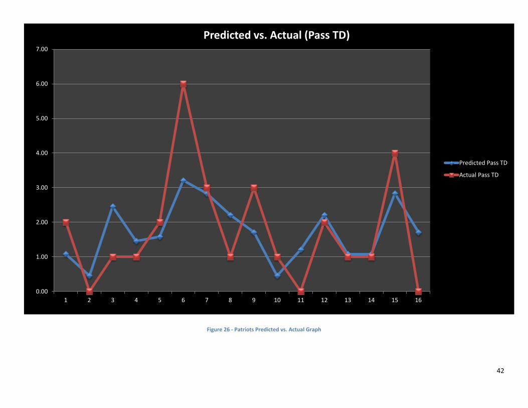
method versus AccuScore’s projection method.

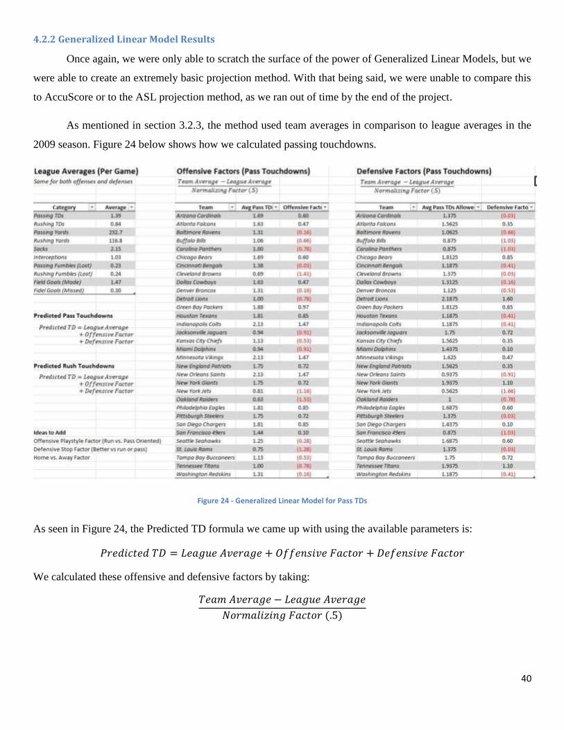
In addition to the play probability method, the project team was also able to generate a

different projection model. Due to Professor Abraham’s experience with predictive modeling in

the insurance industry, we determined that the most accurate way of projecting team statistics for

a season is through Generalized Linear Models (GLMs). A GLM is a multivariate method that

uses the most important parameters or statistics to predict a future outcome. The GLM method

was developed in an effort to fix some of the issues of one-way analyses, which only took into

account the individual predictor variable affecting a single response variable. Generalized Linear

Models look at the correlation between variables and attempt to display the observed variable, Y,

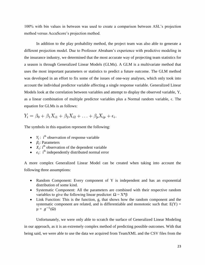
as a linear combination of multiple predictor variables plus a Normal random variable, ϵ. The

equation for GLMs is as follows:

The symbols in this equation represent the following:

: ith

observation of response variable

: Parameters

: ith

observation of the dependent variable

: ith

independently distributed normal error

A more complex Generalized Linear Model can be created when taking into account the

following three assumptions:

Random Component: Every component of Y is independent and has an exponential

distribution of some kind.

Systematic Component: All the parameters are combined with their respective random

variables to give the following linear predictor: Ω = X*β

Link Function: This is the function, g, that shows how the random component and the

systematic component are related, and is differentiable and monotonic such that: E(Y) =

µ = (Ω)

Unfortunately, we were only able to scratch the surface of Generalized Linear Modeling

in our approach, as it is an extremely complex method of predicting possible outcomes. With that

being said, we were able to use the data we acquired from TeamXML and the CSV files from the

24

play probability trees as different parameters for our prediction method. Many of the parameters

we used involved taking a team’s average in a single category in relation to the league average in

that same category. For example, say passing yards is the category we want to project. One of the

parameters would be the league average for passing yards. A second parameter would take into

account how the team does in relation to the league average and adding or subtracting a number

depending on if they were better or worse than that league average. A third parameter would

factor in the defense that was being played against during the game and its relation to the league

average (does it allow more passing yards than the league average or does it allow less). From

these three parameters, we were able to generate projections for each game.

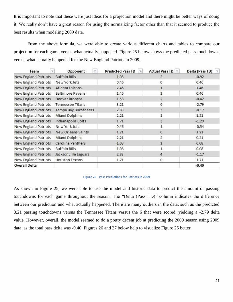
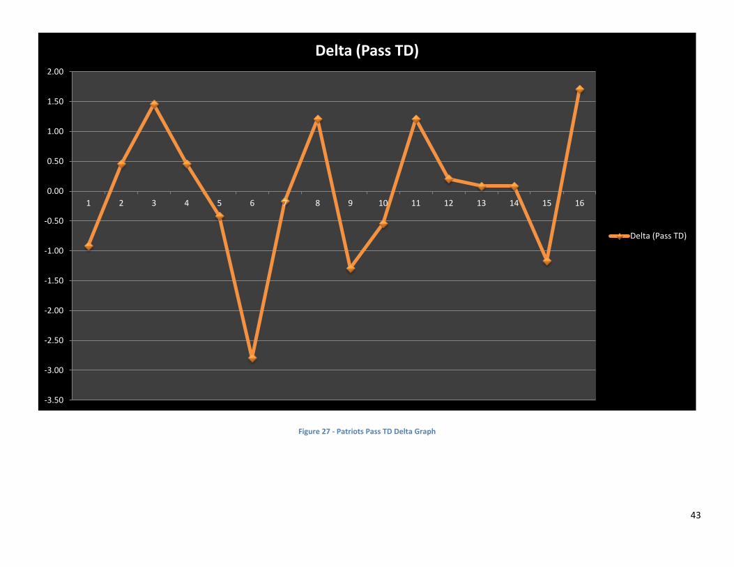
3.2.4 Phase 4: Documentation of Results

Phase 4 was fairly straight forward, as it involved looking at each projection method and

documenting the results. Much of this documentation was used in the creation of the results

section for Objective 2.

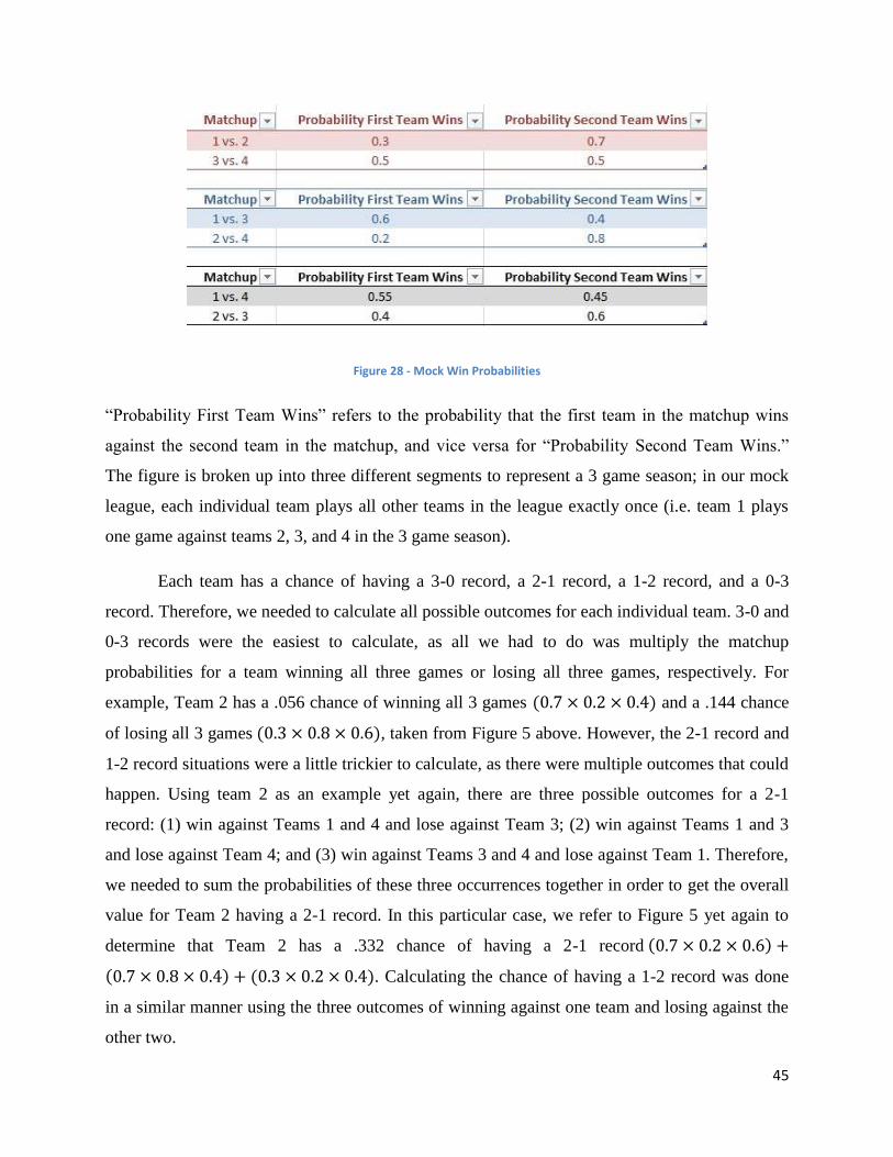
3.3 Objective 3: Reviewing and Refining Win Probability Methods

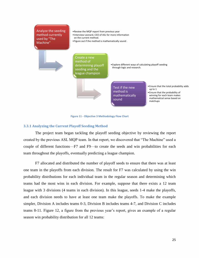
Reviewing and refining playoff seeding and win probability methods involved three

primary tasks: (1) Analyzing the method currently used by “The Machine” to determine the

league champion; (2) Creating a new method of determining the league champion; and (3)

Testing if the new method works from a mathematical standpoint. These tasks and their

associated subtasks are outlined in Figure 11 below:

25

Figure 11 - Objective 3 Methodology Flow Chart

3.3.1 Analyzing the Current Playoff Seeding Method

The project team began tackling the playoff seeding objective by reviewing the report

created by the previous ASL MQP team. In that report, we discovered that “The Machine” used a

couple of different functions—F7 and F9—to create the seeds and win probabilities for each

team throughout the playoffs, eventually predicting a league champion.

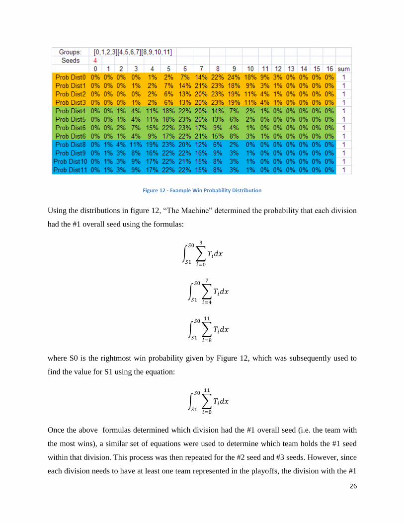
F7 allocated and distributed the number of playoff seeds to ensure that there was at least

one team in the playoffs from each division. The result for F7 was calculated by using the win

probability distributions for each individual team in the regular season and determining which

teams had the most wins in each division. For example, suppose that there exists a 12 team

league with 3 divisions (4 teams in each division). In this league, seeds 1-4 make the playoffs,

and each division needs to have at least one team make the playoffs. To make the example

simpler, Division A includes teams 0-3, Division B includes teams 4-7, and Division C includes

teams 8-11. Figure 12, a figure from the previous year’s report, gives an example of a regular

season win probability distribution for all 12 teams:

Analyze the seeding method currently used by "The Machine"

•Review the MQP report from previous year

•Interview Leonard, CEO of ASL for more information on the current method.

•Figure out if the method is mathematically sound .

Create a new method of determining playoff seeding and the league champion

•Explore different ways of calculating playoff seeding through logic and research.

Test if the new method is mathematically sound

•Ensure that the total probability adds up to 1

•Ensure that the probability of winning for each team makes mathematical sense based on matchups

26

Figure 12 - Example Win Probability Distribution

Using the distributions in figure 12, “The Machine” determined the probability that each division

had the #1 overall seed using the formulas:

∫ ∑

∫ ∑

∫ ∑

where S0 is the rightmost win probability given by Figure 12, which was subsequently used to

find the value for S1 using the equation:

∫ ∑

Once the above formulas determined which division had the #1 overall seed (i.e. the team with

the most wins), a similar set of equations were used to determine which team holds the #1 seed

within that division. This process was then repeated for the #2 seed and #3 seeds. However, since

each division needs to have at least one team represented in the playoffs, the division with the #1

27

overall seed cannot have the #2 overall seed or the #3 overall seed. Of course, this formula

changes depending on the set of rules used by each league. Leagues may allow for the best

overall teams to make the playoffs regardless of division, as well as have a different number of

divisions and teams allowed to make the playoffs. In our example, one additional team makes the

playoffs, which is determined by the formula below:

∑∫

The above summation essentially says that the team with the highest win probability distribution

will be the one that makes the playoffs. The 4th

seed to make the playoffs is not dependent on the

division.

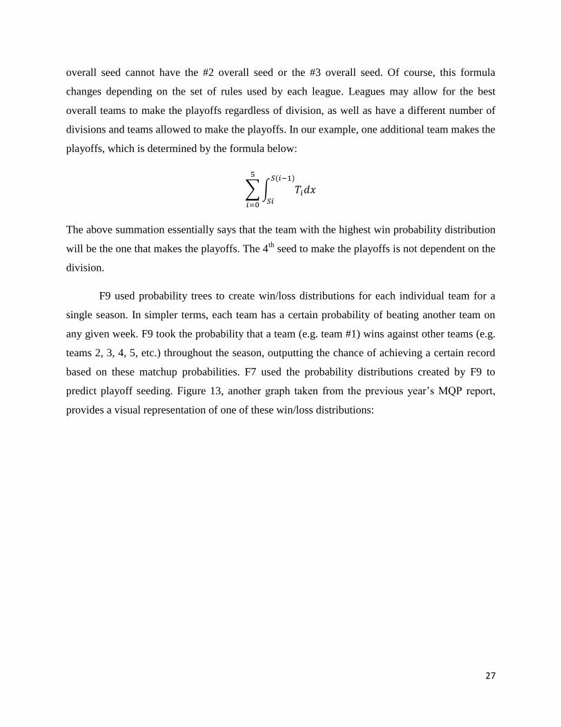
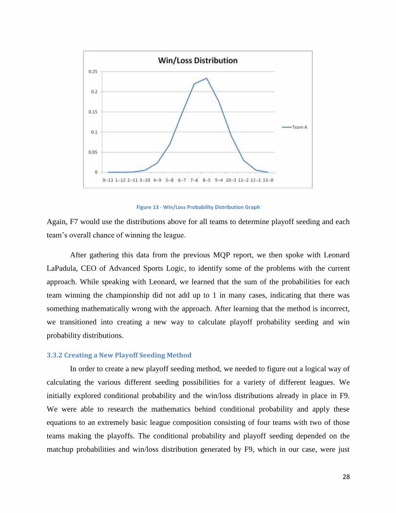
F9 used probability trees to create win/loss distributions for each individual team for a

single season. In simpler terms, each team has a certain probability of beating another team on

any given week. F9 took the probability that a team (e.g. team #1) wins against other teams (e.g.

teams 2, 3, 4, 5, etc.) throughout the season, outputting the chance of achieving a certain record

based on these matchup probabilities. F7 used the probability distributions created by F9 to

predict playoff seeding. Figure 13, another graph taken from the previous year’s MQP report,

provides a visual representation of one of these win/loss distributions:

28

Figure 13 - Win/Loss Probability Distribution Graph

Again, F7 would use the distributions above for all teams to determine playoff seeding and each

team’s overall chance of winning the league.

After gathering this data from the previous MQP report, we then spoke with Leonard

LaPadula, CEO of Advanced Sports Logic, to identify some of the problems with the current

approach. While speaking with Leonard, we learned that the sum of the probabilities for each

team winning the championship did not add up to 1 in many cases, indicating that there was

something mathematically wrong with the approach. After learning that the method is incorrect,

we transitioned into creating a new way to calculate playoff probability seeding and win

probability distributions.

3.3.2 Creating a New Playoff Seeding Method

In order to create a new playoff seeding method, we needed to figure out a logical way of

calculating the various different seeding possibilities for a variety of different leagues. We

initially explored conditional probability and the win/loss distributions already in place in F9.

We were able to research the mathematics behind conditional probability and apply these

equations to an extremely basic league composition consisting of four teams with two of those

teams making the playoffs. The conditional probability and playoff seeding depended on the

matchup probabilities and win/loss distribution generated by F9, which in our case, were just

29

made up to find a new method. The results and problems from the conditional probability

method are outlined in section 4.3.

Upon meeting with Leonard yet again to discuss a new playoff seeding method, we

determined that generating all possible outcomes for playoff seeding did not factor into

predicting the league champion once a league hit the playoffs. Since the playoff seeds were

already determined by that time, we were able to come up with a much simpler method using the

matchup probabilities for each team. The results are outlined in section 4.3.

3.3.3 Testing the Method

With a new method of determining the probability that a team wins the championship

created, we still needed to test if the method made mathematical sense. This was a rather simple

task, as all we had to do was ensure that the sum of all individual probabilities added up to 1. To

test this methodwe generated mock matchup probabilities and calculated each team’s chance of

becoming the league champion. We then added up all of these probabilities to determine if the

method worked or not.

30

4. Results from New Calculation Methods

4.1 Increased Accuracy on Probability Distribution Results

While we didn’t necessarily solve the issue of upper tier players having downside and

lower tier players having upside, we were able to create a base for weighting which projections

matter to the user, as well as verify Advanced Sports Logic’s “Shape shifting” method, which

begins to take into account tiers of players.

4.1.1 Accuracy and Precision

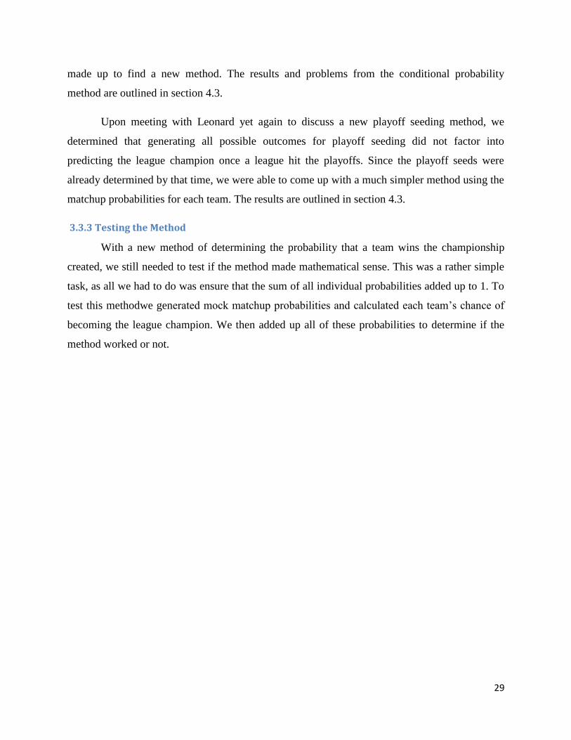
As mentioned in section 3.1.1, we used the Excel file with AccuScore’s predictions to

generate accuracy and precision. The predicted value subtracted from the actual value gave the

accuracy for each projection, whereas precision was measured as the standard deviation between

predictions from week to week.

Accuracy was broken down into two separate areas: (1) Proximity Accuracy and (2)

Overall Accuracy. Figure 14 below shows both the Proximity Accuracy and Overall Accuracy.

Figure 14 - Proximity and Overall Accuracy Example

As seen by Figure 14, the Proximity Accuracy is simply the diagonal of the Overall Accuracy

matrix. The Proximity Accuracy is the predicted value subtracted from the actual value the week

before the game actually happens for each player. The Overall Accuracy takes into account the

accuracy of all predictions throughout the season, no matter how far in the future they are. The

Overall Accuracy gives the larger picture on how accurate the predictions are throughout the

season. Negative numbers mean that AccuScore underestimated with their prediction, whereas

positive numbers mean that AccuScore overestimated with their prediction.

31

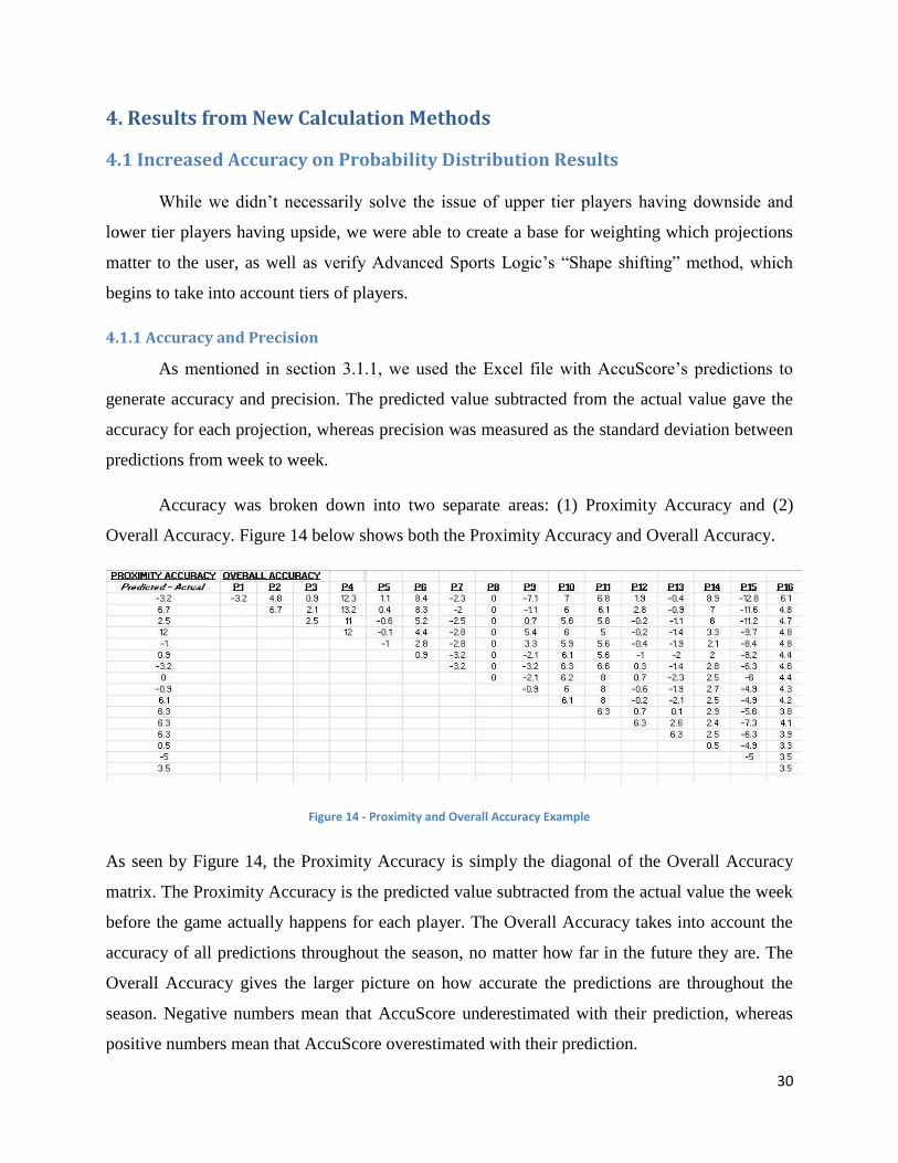
After accuracy was calculated, we then calculated precision. Figure 15 below gives an

example of the precision calculations.

Figure 15 - Precision Example

The precision shows how much the predictions varied from week to week. Of course, since there

is only one prediction in the P1 column in Figure 15, no standard deviation can be calculated for

that week.

While these calculations are neat (for lack of a better word), we were not able to decipher

what they meant in the larger picture of things. Yes, these calculations do show how much the

predictions varied from what actually happened and how much they changed over the course of

time. However, we did not have anything to compare the accuracy and precision to. For example,

if the summation of the overall accuracy for a single player was 50, who is to say that is good or

bad with no other predictions and accuracy measurements to compare it to?

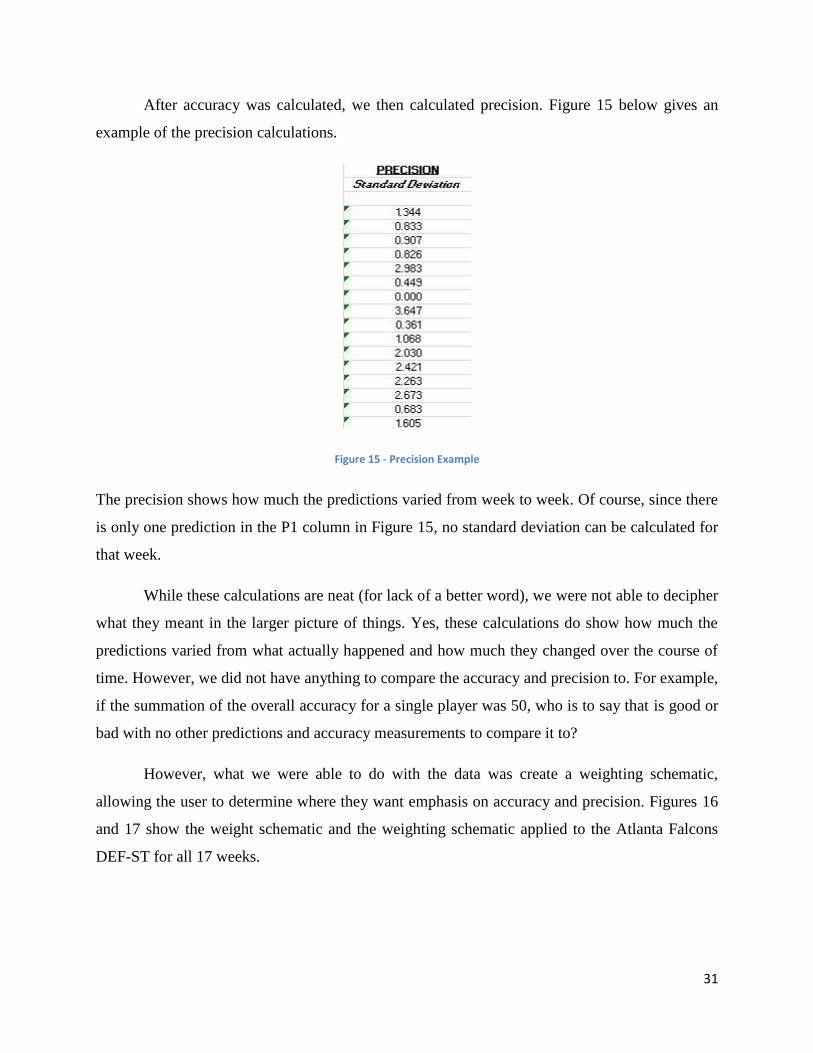
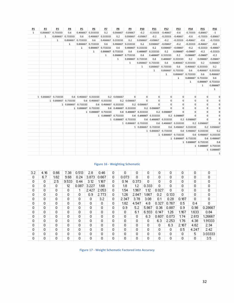
However, what we were able to do with the data was create a weighting schematic,

allowing the user to determine where they want emphasis on accuracy and precision. Figures 16

and 17 show the weight schematic and the weighting schematic applied to the Atlanta Falcons

DEF-ST for all 17 weeks.

32

Figure 16 - Weighting Schematic

Figure 17 - Weight Schematic Factored into Accuracy

33

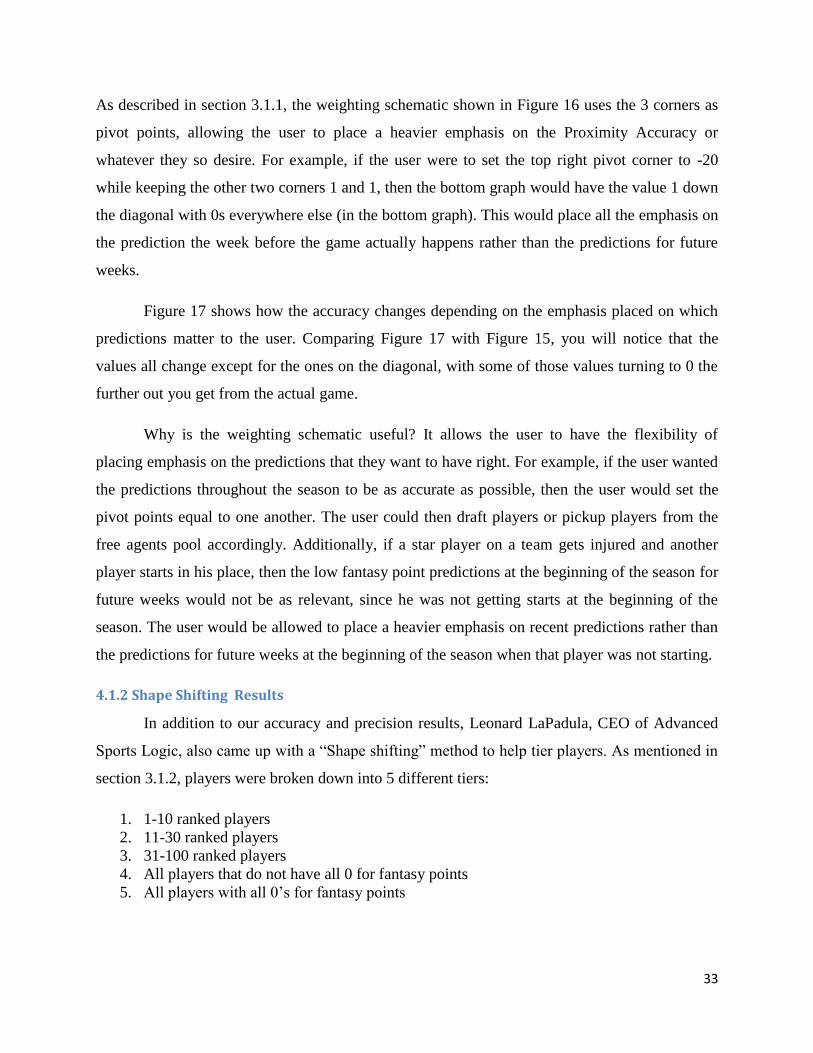
As described in section 3.1.1, the weighting schematic shown in Figure 16 uses the 3 corners as

pivot points, allowing the user to place a heavier emphasis on the Proximity Accuracy or

whatever they so desire. For example, if the user were to set the top right pivot corner to -20

while keeping the other two corners 1 and 1, then the bottom graph would have the value 1 down

the diagonal with 0s everywhere else (in the bottom graph). This would place all the emphasis on

the prediction the week before the game actually happens rather than the predictions for future

weeks.

Figure 17 shows how the accuracy changes depending on the emphasis placed on which

predictions matter to the user. Comparing Figure 17 with Figure 15, you will notice that the

values all change except for the ones on the diagonal, with some of those values turning to 0 the

further out you get from the actual game.

Why is the weighting schematic useful? It allows the user to have the flexibility of

placing emphasis on the predictions that they want to have right. For example, if the user wanted

the predictions throughout the season to be as accurate as possible, then the user would set the

pivot points equal to one another. The user could then draft players or pickup players from the

free agents pool accordingly. Additionally, if a star player on a team gets injured and another

player starts in his place, then the low fantasy point predictions at the beginning of the season for

future weeks would not be as relevant, since he was not getting starts at the beginning of the

season. The user would be allowed to place a heavier emphasis on recent predictions rather than

the predictions for future weeks at the beginning of the season when that player was not starting.

4.1.2 Shape Shifting Results

In addition to our accuracy and precision results, Leonard LaPadula, CEO of Advanced

Sports Logic, also came up with a “Shape shifting” method to help tier players. As mentioned in

section 3.1.2, players were broken down into 5 different tiers:




4. All players that do not have all 0 for fantasy points

5. All players with all 0’s for fantasy points

34

The tiers were determined by the predicted fantasy points scored by the player throughout the

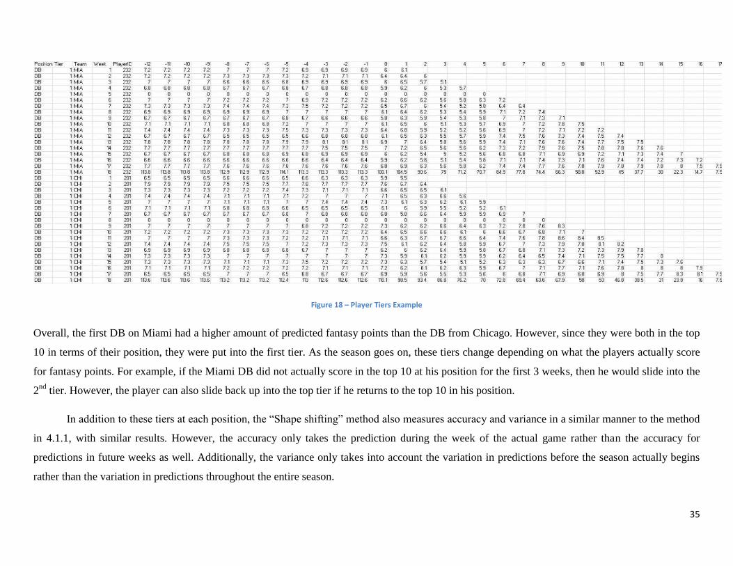
season. To help better illustrate the tier system, let us look at an example in Figure 18.

35

Figure 18 – Player Tiers Example

Overall, the first DB on Miami had a higher amount of predicted fantasy points than the DB from Chicago. However, since they were both in the top

10 in terms of their position, they were put into the first tier. As the season goes on, these tiers change depending on what the players actually score

for fantasy points. For example, if the Miami DB did not actually score in the top 10 at his position for the first 3 weeks, then he would slide into the

2nd

tier. However, the player can also slide back up into the top tier if he returns to the top 10 in his position.

In addition to these tiers at each position, the “Shape shifting” method also measures accuracy and variance in a similar manner to the method

in 4.1.1, with similar results. However, the accuracy only takes the prediction during the week of the actual game rather than the accuracy for

predictions in future weeks as well. Additionally, the variance only takes into account the variation in predictions before the season actually begins

rather than the variation in predictions throughout the entire season.

36

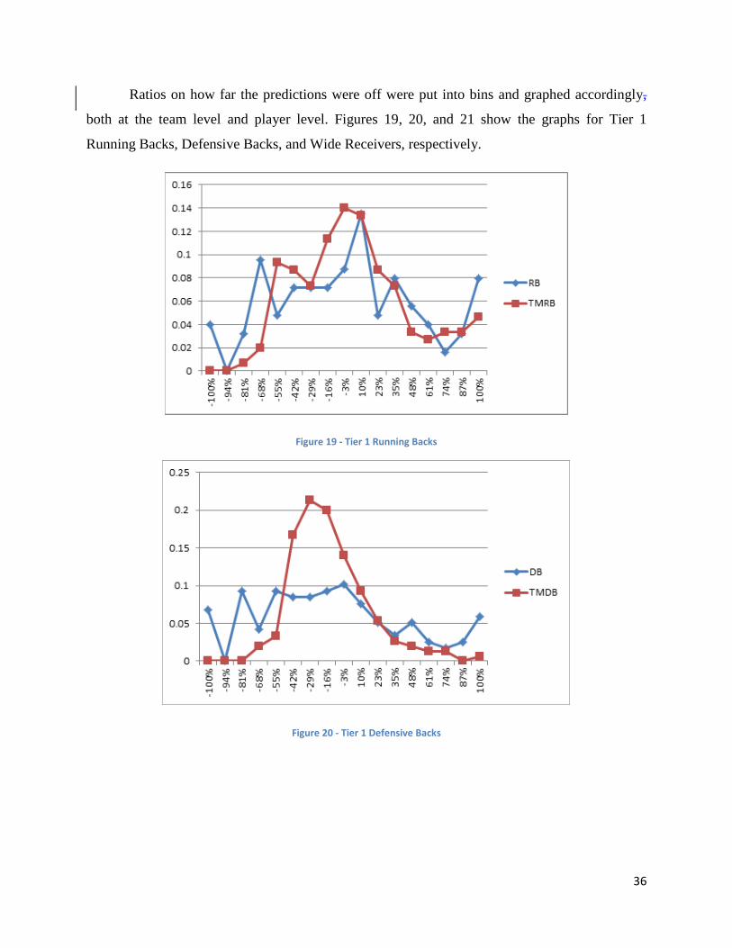
Ratios on how far the predictions were off were put into bins and graphed accordingly,

both at the team level and player level. Figures 19, 20, and 21 show the graphs for Tier 1

Running Backs, Defensive Backs, and Wide Receivers, respectively.

Figure 19 - Tier 1 Running Backs

Figure 20 - Tier 1 Defensive Backs

37

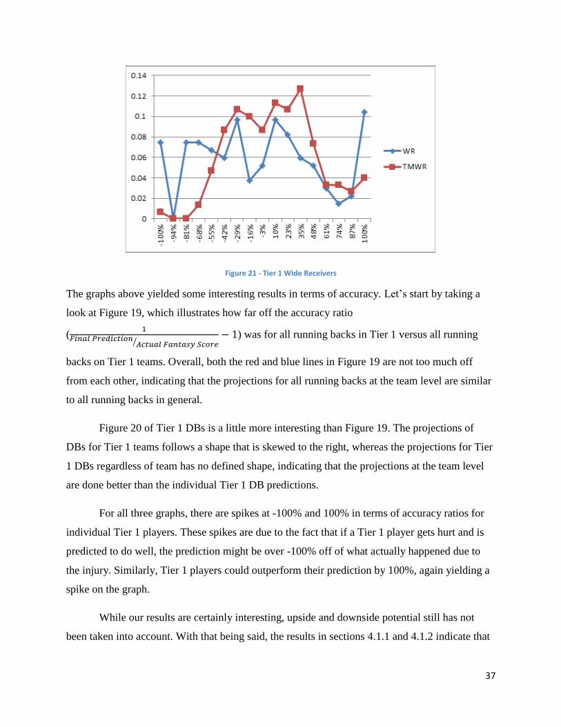
Figure 21 - Tier 1 Wide Receivers

The graphs above yielded some interesting results in terms of accuracy. Let’s start by taking a

look at Figure 19, which illustrates how far off the accuracy ratio

(

⁄

) was for all running backs in Tier 1 versus all running

backs on Tier 1 teams. Overall, both the red and blue lines in Figure 19 are not too much off

from each other, indicating that the projections for all running backs at the team level are similar

to all running backs in general.

Figure 20 of Tier 1 DBs is a little more interesting than Figure 19. The projections of

DBs for Tier 1 teams follows a shape that is skewed to the right, whereas the projections for Tier

1 DBs regardless of team has no defined shape, indicating that the projections at the team level

are done better than the individual Tier 1 DB predictions.

For all three graphs, there are spikes at -100% and 100% in terms of accuracy ratios for

individual Tier 1 players. These spikes are due to the fact that if a Tier 1 player gets hurt and is

predicted to do well, the prediction might be over -100% off of what actually happened due to

the injury. Similarly, Tier 1 players could outperform their prediction by 100%, again yielding a

spike on the graph.

While our results are certainly interesting, upside and downside potential still has not

been taken into account. With that being said, the results in sections 4.1.1 and 4.1.2 indicate that

38

ASL is on its way to being able to allow for a tier system that allows the user to see the upside

and downside potential for each player.

4.2 Projection Modeling Results

While Advanced Sports Logic and the project team were able to generate a couple of

different projection methods, it is important to note that a lot more can be done to increase the

accuracy of the projections and make more intricate mathematical models. With that being said,

let us examine some of the results.

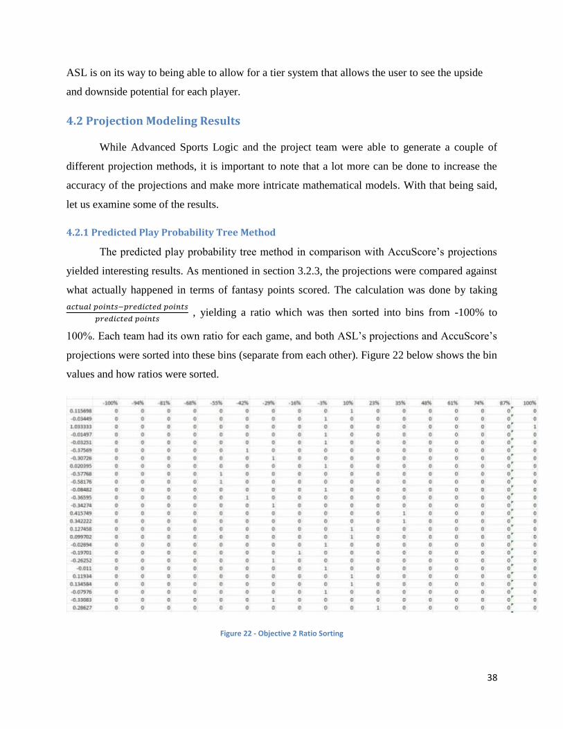
4.2.1 Predicted Play Probability Tree Method

The predicted play probability tree method in comparison with AccuScore’s projections

yielded interesting results. As mentioned in section 3.2.3, the projections were compared against

what actually happened in terms of fantasy points scored. The calculation was done by taking

, yielding a ratio which was then sorted into bins from -100% to

100%. Each team had its own ratio for each game, and both ASL’s projections and AccuScore’s

projections were sorted into these bins (separate from each other). Figure 22 below shows the bin

values and how ratios were sorted.

Figure 22 - Objective 2 Ratio Sorting

39

As shown in Figure 22, a value of .115698 would be sorted into the bin from 10% to 23%, a -.03449 ratio would

be sorted into the ratio from -16% to -3%, so on and so forth.

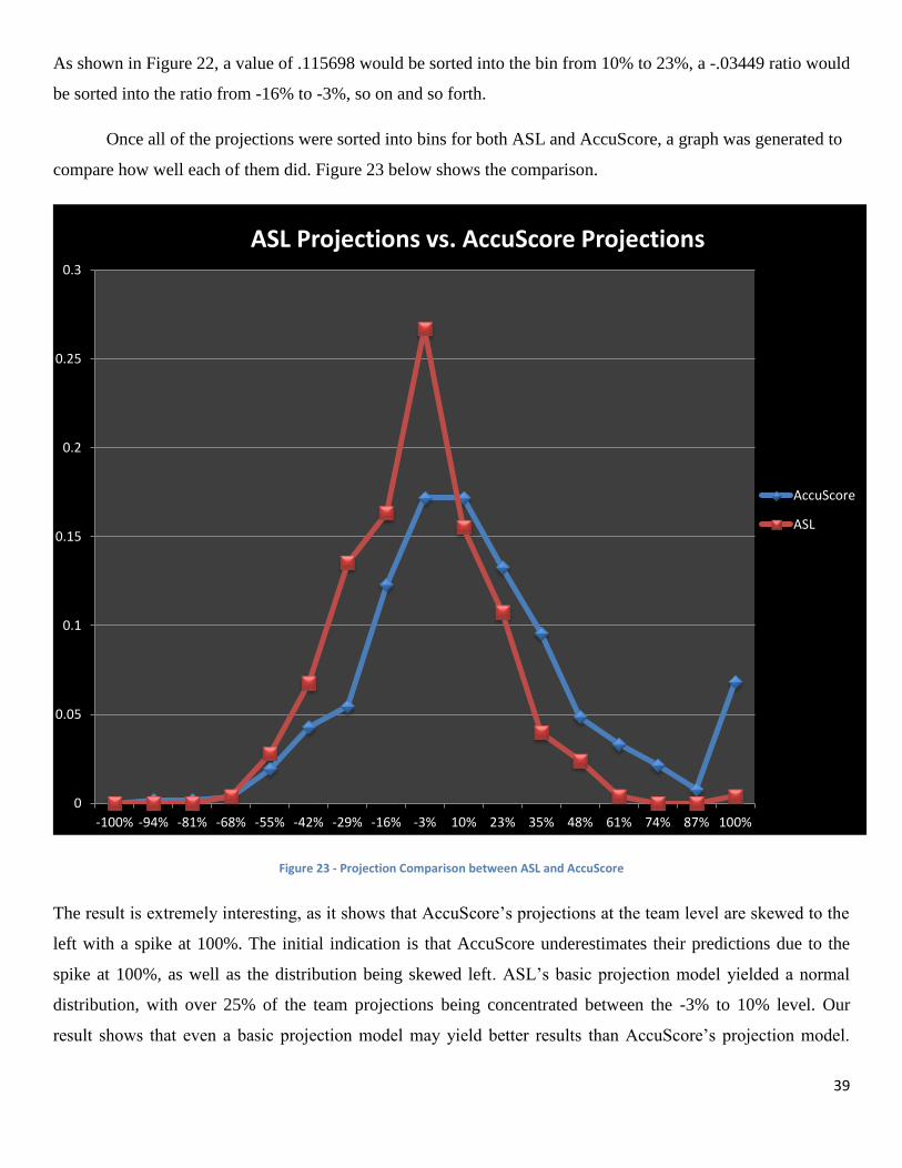
Once all of the projections were sorted into bins for both ASL and AccuScore, a graph was generated to

compare how well each of them did. Figure 23 below shows the comparison.

Figure 23 - Projection Comparison between ASL and AccuScore

The result is extremely interesting, as it shows that AccuScore’s projections at the team level are skewed to the

left with a spike at 100%. The initial indication is that AccuScore underestimates their predictions due to the

spike at 100%, as well as the distribution being skewed left. ASL’s basic projection model yielded a normal

distribution, with over 25% of the team projections being concentrated between the -3% to 10% level. Our

result shows that even a basic projection model may yield better results than AccuScore’s projection model.

0

0.05

0.1

0.15

0.2

0.25

0.3

-100% -94% -81% -68% -55% -42% -29% -16% -3% 10% 23% 35% 48% 61% 74% 87% 100%

ASL Projections vs. AccuScore Projections

AccuScore

ASL

40

4.2.2 Generalized Linear Model Results

Once again, we were only able to scratch the surface of the power of Generalized Linear Models, but we

were able to create an extremely basic projection method. With that being said, we were unable to compare this

to AccuScore or to the ASL projection method, as we ran out of time by the end of the project.

As mentioned in section 3.2.3, the method used team averages in comparison to league averages in the

2009 season. Figure 24 below shows how we calculated passing touchdowns.

Figure 24 - Generalized Linear Model for Pass TDs

As seen in Figure 24, the Predicted TD formula we came up with using the available parameters is:

We calculated these offensive and defensive factors by taking:

41

It is important to note that these were just ideas for a projection model and there might be better ways of doing

it. We really don’t have a great reason for using the normalizing factor other than that it seemed to produce the

best results when modeling 2009 data.

From the above formula, we were able to create various different charts and tables to compare our

projection for each game versus what actually happened. Figure 25 below shows the predicted pass touchdowns

versus what actually happened for the New England Patriots in 2009.

Figure 25 - Pass Predictions for Patriots in 2009

As shown in Figure 25, we were able to use the model and historic data to predict the amount of passing

touchdowns for each game throughout the season. The “Delta (Pass TD)” column indicates the difference

between our prediction and what actually happened. There are many outliers in the data, such as the predicted

3.21 passing touchdowns versus the Tennessee Titans versus the 6 that were scored, yielding a -2.79 delta

value. However, overall, the model seemed to do a pretty decent job at predicting the 2009 season using 2009

data, as the total pass delta was -0.40. Figures 26 and 27 below help to visualize Figure 25 better.

42

Figure 26 - Patriots Predicted vs. Actual Graph

0.00

1.00

2.00

3.00

4.00

5.00

6.00

7.00

1 2 3 4 5 6 7 8 9 10 11 12 13 14 15 16

Predicted vs. Actual (Pass TD)

Predicted Pass TD

Actual Pass TD

43

Figure 27 - Patriots Pass TD Delta Graph

-3.50

-3.00

-2.50

-2.00

-1.50

-1.00

-0.50

0.00

0.50

1.00

1.50

2.00

1 2 3 4 5 6 7 8 9 10 11 12 13 14 15 16

Delta (Pass TD)

Delta (Pass TD)

44

Figure 27 is of particular interest, as it really shows how much the model varied from week to

week. 9 of the 16 games played were within 1 touchdown of what actually happened, with 7 of

those 9 games being within 0.5 touchdowns of what actually happened.

Obviously, the results section only shows how the model did for one team. We ended up

testing it with a few other teams (Giants, Bills, Vikings), and the model seemed to be fairly

accurate in its overall delta with the exception of the Vikings. However, additional factors may

be able to be added in to increase the overall accuracy of the Generalized Linear Model

including, but not limited to:

Offensive play style (run vs. pass oriented)

Defensive stop factor (better vs. run or pass)

Home vs. away factor

Indoor vs. outdoor factor

Weather factor

Additionally, the main problem with the model right now is that it uses 2009 data to predict what

happened in 2009. In other words, we have not figured out a way to use the model to predict

what would have happened in 2010 just yet. As such, much more investigation is needed.

4.3 Win Probability Results

Overall, we were able to analyze the current playoff seeding method, show that the

current method has mathematical inaccuracies, and create a couple of different attempts at a new

method, one of which was much simpler than the other.

4.3.1 Results of the Current Method

In order to verify Leonard’s claim regarding the mathematical inaccuracy of F7—the

current playoff seeding method—we began by creating a simplified league with four teams. We

assigned mock probabilities for each team winning against another team, which can be seen in

Figure 28 below:

45

Figure 28 - Mock Win Probabilities

“Probability First Team Wins” refers to the probability that the first team in the matchup wins

against the second team in the matchup, and vice versa for “Probability Second Team Wins.”

The figure is broken up into three different segments to represent a 3 game season; in our mock

league, each individual team plays all other teams in the league exactly once (i.e. team 1 plays

one game against teams 2, 3, and 4 in the 3 game season).

Each team has a chance of having a 3-0 record, a 2-1 record, a 1-2 record, and a 0-3

record. Therefore, we needed to calculate all possible outcomes for each individual team. 3-0 and

0-3 records were the easiest to calculate, as all we had to do was multiply the matchup

probabilities for a team winning all three games or losing all three games, respectively. For

example, Team 2 has a .056 chance of winning all 3 games and a .144 chance

of losing all 3 games , taken from Figure 5 above. However, the 2-1 record and

1-2 record situations were a little trickier to calculate, as there were multiple outcomes that could

happen. Using team 2 as an example yet again, there are three possible outcomes for a 2-1

record: (1) win against Teams 1 and 4 and lose against Team 3; (2) win against Teams 1 and 3

and lose against Team 4; and (3) win against Teams 3 and 4 and lose against Team 1. Therefore,

we needed to sum the probabilities of these three occurrences together in order to get the overall

value for Team 2 having a 2-1 record. In this particular case, we refer to Figure 5 yet again to

determine that Team 2 has a .332 chance of having a 2-1 record

. Calculating the chance of having a 1-2 record was done

in a similar manner using the three outcomes of winning against one team and losing against the

other two.

46

From this mock league, we were able to create a win/loss probability distribution for each

team, which were simpler versions of the distributions created by F9 in leagues with a greater

number of teams. Figure 29 below shows a visual representation of the win/loss probability

distribution for Team 2 in our mock league.

Figure 29 - Mock Win/Loss Probability Distribution

Again, Team 2 had a .056 chance of going 3-0, a .332 chance of going 2-1, a .468 chance of

going 1-2, and a .144 chance of going 0-3. With these win/loss probability distributions in hand,

we transitioned into tackling the problem with the current playoff seeding method.

Using the win/loss probability distributions for all 4 teams in our mock league, we were

able to create a stacked graph to better understand what “The Machine” was doing. Figure 30

below represents the combined win/loss probability distributions for all 4 teams.

0

0.05

0.1

0.15

0.2

0.25

0.3

0.35

0.4

0.45

0.5

0.056

0.332

0.468

0.144

Team 2 - Win/Loss Probability Distribution

3-0

2-1

1-2

0-3

47

Figure 30 - Stacked Win/Loss Probability Distribution

The current win probability method takes the sum of all 4 teams going 3-0 and “splices” off a

part of all 4 teams going 2-1 until the 3-0 probability adds up to 1. In this case, the sum of all 4

teams going 3-0 is .455, meaning that an additional .545 needs to be taken from 2-1. The splice is

done by taking the area of the rectangle (height is the sum of all 2-1 records, base is unknown)

and setting it equal to the .545 value , yielding a base value of .355. To find

the individual probability “spliced” off of each team, the base value of .355 is multiplied by the

individual height of each different colored rectangle. For example, the probability taken from the

2-1 portion for Team 4 is , which is .158. Done for all 4 teams,

does in fact equate to what we’re looking for, .545. The process is repeated to fill in

0

0.2

0.4

0.6

0.8

1

1.2

1.4

1.6

3-0 2-1 1-2 0-3

Team 4 0.18 0.445 0.32 0.055

Team 3 0.12 0.38 0.38 0.12

Team 2 0.056 0.332 0.468 0.144

Team 1 0.099 0.378 0.397 0.126

Win/Loss Probability Distribution

Team 4

Team 3

Team 2

Team 1

48

the probabilities for 2-1, 1-2, and 0-3, which eventually creates a new distribution for each team

being a certain seed in the playoffs.

Where the method fell apart is when the actual playoff seeding and chance of winning the

championship was determined. To make this explanation simpler, we will not be using the

numbers from Figures 28, 29, and 30, although we will still be examining a 4-team league with 2

playoff seeds. Figure 31 represents each individual team’s chance of being seed 1 or seed 2 in the

playoffs.

Figure 31 - Chance of Being a Certain Seed

Again, these probabilities would normally be determined by the “splicing” method, but in our

sample case, they are made up for simplicity. The playoff seeding method in place assumed that

being seed 1 or being seed 2 was independent of each other. The method added up the

probabilities of being either of the two seeds, along with the probability remaining for the other

teams being either of the two seeds, yielding Figure 32 below.

Figure 32 - Chance for Other Teams to Be a Certain Seed

The method then calculated the chance for each team to play one of the other teams in the

playoffs. For example, Team 1 has a .57 probability of being the 1st or 2

nd seed. Team 2 has 1.64

probability remaining, Team 3 has 1.43 probability remaining, and Team 4 has a 1.5 probability

remaining. The method used by “The Machine” takes ⁄ , ⁄ , and ⁄ to

49

calculate Team 1’s chance of playing Team 2, Team 3, or Team 4 respectively. The four team

method has been extrapolated to work for more than four teams and more than two playoff seeds.

Once these probabilities are calculated for all teams, the “chance of playing Team X”

probabilities are then multiplied by the matchup probabilities to determine each team’s chance of

winning against the other team. The probabilities are summed together to determine each team’s

chance of winning the championship. Figures 33 and 34 below show this process.

Figure 33 - Mock Matchup Probabilities

Figure 34 - Chance of Winning Championship (Current Method)

Figure 33 shows made up matchup probabilities for each team beating the other team. Figure 34

shows the “chance of playing Team X” probabilities multiplied by these matchup probabilities.

The “sum” column in Figure 33 shows the overall chance for each team to win the

championship. However, as already mentioned, the total sum adds up to something greater than

1, indicating that there is a problem with this method.

We were able to determine that the main problem with this method was the fact that it

assumed the seeding was independent of each other, which was not actually true. The chance of

being the 1st seed is directly tied to the chance of being the 2

nd seed, as a team cannot be both

seeds at the same time. Therefore, we moved onto finding a new way to calculate the chance of

winning the championship.

50

4.3.2 Results from the New Win Probability Method

In order to account for depending seeding, we created a method using conditional

probability and tested it in a 6-team, 2-seed league similar to the league used to test the original

method. Figure 35 below shows the probabilities for each team to be the 1st seed or 2

nd seed in

the playoffs.

Figure 35 - New Seeding Probabilities

Again, the seeding would normally be determined from the win/loss probability distributions for

each team and the “splicing” method, but for simplicity, they are purely made up for this

example. Using these seeding probabilities, we then were able to calculate the possibility that

other teams were either the 1st or 2

nd seed. Figure 36 helps to better explain this:

Figure 36 - New Remaining Seed Method

Essentially, we just took , where n = 1, 2 for each team to find the chance for all other

teams to be the 1st or 2

nd seed. With a table like figure 36 calculated, we were then able to use

51

conditional probability to calculate the chance of playing a certain team in the playoffs. Figure

37 shows the chance for each team to play each other in the playoffs.

Figure 37 - Chance to Play Team X

To help better illustrate this method, let us use the example of t1 playing t2, the outlined box in

Figure 37. We took the probability of t1 being the 1st seed, which is .07 given by Figure 12, and

multiplied that probability by the probability of t2 being the 2nd

seed, which is .25 given by

Figure 12 again. We then divided this number by the chance for other teams to be the 2nd

seed (t1

is the 1st seed), .68 given by Figure 35, giving us the final result of .03. Of course, we also had to

do the flipside of this where t2 is the 1st seed and t1 is the 2

nd seed, which is .10 given by Figure

14 above (down one cell and left one cell). We then multiplied these “chance of playing Team

X” probabilities by the matchup probabilities, illustrated by Figure 38 below.

52

Figure 38 - New Chance of Winning Championship

Two charts were used to account for each team’s probabilities of beating the other team. For

example, if t1 has a .8 chance of beating t2, then t2 has a .2 chance of beating t1. Since both

cases need to be considered, two charts were created to use these matchup probabilities. As

Figure 38 illustrates, the overall probability sums to 1, indicating that the conditional probability

method is more mathematically accurate than the previous method.

Once we had the conditional probability method in place, we generated formulas for a

simple case consisting of 4-teams and 2-seeds:

Let n = 1, 2, 3, 4 represent the team number. Then there exists some matrix

such that

53

where n = 1, 2, … , 6 are probabilities for each matchup (i.e. is the probability of

winning versus , is the probability of winning versus , is the probability of

winning versus , etc).

Let m = 1, 2 represent the seeds for the playoffs. Then there exists some

matrix such that

where i = 1, 3, 5, 7 are the probabilities for each team being in the playoffs, and j = 2,

4, 6, 8 are the probabilities for each team being in the playoffs (i.e. and are the

probabilities for being seed #1 and seed #2, respectively, and are the probabilities for

being seed #1 and seed #2, respectively, etc).

Since the probability that is are dependent events (i.e. cannot be both and

), then the rules of conditional probability apply ( =

). Thus, there exists the

chance that is not (i.e. is not = , is not = , etc).

Using conditional probability, we can generate the chance that each team has of playing

each other in the playoffs. To solve, we need to exam all possible cases that a team makes the

playoffs as where m = 1,2 in this case. Therefore, as the first seed (m = 1), has the

conditional probability of playing a different n = 2, 3, 4 such that

where j = 4, 6, 8. As the second seed (m = 2), has the conditional probability of playing a

different n = 2, 3, 4 such that

where . These equations give the conditional probability for making the playoffs as

both the 1st and 2

nd seed ( where m = 1,2), as well as the probability that matches up with

each of the teams. If the calculations are done for all teams, then the conditional probability adds

to 1 for both of the equations above.

Next, we need to calculate the probability that a team actually wins the championship. To

solve, we take the conditional probabilities and multiply them by the probability that a team has

of winning against a different team. For , we take

54

where n = 1, 2, 4 resulting in the probability of winning against where n = 2, 3, 4 with as

either the #1 or #2 seed. In other words, summing these two equations will give us the overall

probability of winning the championship factoring in both the conditional probability of

making the playoffs as well as the probability of winning against each team. Done for all teams,

the total probability adds to 1.

While we were able to generate these formulas for an extremely basic case, we ran into a

lot of trouble creating formulas for more complex cases. More teams, more seeds, and different

divisions presented difficulties, as there were more and more matchup possibilities to take into

account. We were stuck for a while trying to figure out how to take all of these possibilities into

account.

However, what we eventually realized is that the playoff seeds are determined by the

time the playoffs start, meaning that we really didn’t have to worry about the various different

combinations of playoff seeds. We simply used the matchup probabilities multiplied together to

generate the overall chance for a team to win the league.

For example, in a 6-team league with 4-seeds, the playoff “bracket” is already

determined. Let us assume that Teams 1-4 make the playoffs, with Team 1 playing Team 4 and

Team 2 playing Team 3. The chance for Team 1 to win the championship is simply its chance of

beating Team 4 multiplied by its chance of beating Team 2 or Team 3. The same method can be

done for the other teams, with the total probability summing to 1. This method is much simpler

and still uses the chance of playing different teams, but discards the different possible playoff

seeds for all teams. The code within “The Machine” for this method is located in Appendix A.

55

5. Conclusions and Recommendations

While we were able to achieve a number of tangible results, a lot of things didn’t really

feel “complete” to us by the conclusion of the projection. However, we were able to draw some

conclusions and have quite a few recommendations for Advance Sports Logic or an MQP team

in future years.

WHILE WE WERE ABLE TO CREATE A WAY TO MEASURE ACCURACY AND

VARIANCE, WE HAVE NOTHING TO COMPARE IT TO.

The method for measuring accuracy and variance is there, but we determined that there

were a few potential scenarios that could happen:

Projections could be pretty close to what actually happened for the entire season, but

could really never be dead on.

Projections could be right on most of the time, but could be way off 1 or 2 weeks,

creating outliers.

Projections could be both right on or way off for the vast majority of the season, but

could be correct during the weeks at the end of the season during the playoffs.

It is extremely difficult to determine which scenario is best, as a lot of it depends on what the

user thinks. The weighting scheme helps to solve this issue. However, we believe that some sort

of grading rubric should be created to give the user the flexibility in determining what they want

and which projections are appropriate for them. Creating this rubric involves using the same

method using different sets of projections and creating a rubric to determine which scenario is

best. Additionally, creating a weighting schematic that allows the user to use non-linear

distributions would allow for even more user flexibility.

THE SHAPE SHIFTING METHOD CREATED DIFFERENT TIERS OF PLAYERS,

BUT DID NOT SOLVE THE ISSUE OF ACCOUNTING FOR UPSIDE AND

DOWNSIDE POTENTIAL.

While we believe that there is a solid method in place in terms of creating player tiers, the

issue at the heart of Objective 1 has not been addressed. Advanced Sports Logic could benefit

from showing that lower tier players have high upside, whereas upper tier players have limited

upside. While Figures 10, 11, and 12 show how far off the accuracy ratios were for Tier 1

Running Backs, Defensive Backs, and Wide Receivers, we struggled in really concluding

anything concrete from the data. We were confused as to why the accuracy ratios only took into

56

account the final prediction and what actually happened rather than all projections, including

those for future weeks. Additionally, we were confused as to why the variance between

predictions only took into account the variation before the season actually began rather than the

full season, as these projections are constantly changing. Further analysis is needed, as creating

non-normal projection distributions for different tiers of players would give Advanced Sports

Logic a leg up on its competitors.

WHILE WE HAVE CREATED A NICE BASE FOR A GENERALIZED LINEAR

MODEL, WE HAVE ONLY SCRATCHED THE SURFACE OF WHAT GLMs CAN DO

AND FURTHER INVESTIGATION IS NEEDED.

We were able to create a method for generating projections at the team level, our method

could be drastically improved by adding additional variables. However, it is important to not

include too many variables in the Generalized Linear Model, since including too many variables

may not tell you how each variable is correlated. A future group can test different ways of

generating these projections using GLMs using factors other than league averages and team

averages to project game statistics.

In addition, the method that we came up with does not really show how “test” variables

are correlated, as we weren’t able to readily find factors such as weather, player age, etc. We

were not able to determine if weather really affects how many pass touchdowns are thrown in a

game, or if home versus away games really affect how team statistics do in any given season. As

a result, a future MQP team can test some of these factors using GLMs to see how the

projections change in relation to what actually happened.

Lastly, the model that we created uses 2009 data to project what will happen in 2009

rather than future years. In other words, we have no way of using 2009 data to model what will

happen in 2010. A future group should look into how to use models to predict what will happen

in future years. It seems to us that no matter what, there will need to be some manual tweaking of

the model to account for what we THINK will happen in a future year. It can be as simple

adjusting team averages based on trades, free agent acquisitions, and the draft to adjust the

overall league average (for our model). However, there are probably many different ways to

adjust the model on a year-to-year basis, and those possibilities should be explored.

57

THE “TOP-DOWN APPROACH” SEEMS TO BE A VALID METHOD FOR

PROJECTIONS, BUT A METHOD FOR DISTRIBUTING THESE TEAM

PROJECTIONS IS NEEDED AT THE INDIVIDUAL LEVEL ONCE THE TEAM

METHOD IS SOLIDIFIED.

First and foremost, the graph created by ASL from the predicted play probability tree

projection model initially indicates that a “top-down approach” to projecting player stats may be

valid. However, we do not really have confirmation of this assumption yet, as we have not

generated a way to project individual player stats from these team stats. Further investigation is

needed to determine whether or not the “top-down approach” really is a valid method of

projecting player statistics.

Additionally, we had a lot of questions regarding how this would translate from the team

level down to the individual level. For example, how are team projections broken up among

players? Is it as simple as assigning a certain percentage to each player and determining that

they’re going to get that percentage of the team statistics on a week-to-week basis? Are there

distributions involved with breaking down team projections to players based on certain

matchups? What happens to team projections if a star player joins a new team? Does this change

how team projections are distributed among individual players on that team? We were not able to

determine the answers to these questions. There certainly appear to be a lot of different ways to

distribute team statistics down to the individual level. As such, further investigation is needed.

THE PLAYOFF SEEDING AND WIN PROBABILITY METHOD WORKS, BUT SEEMS

TOO SIMPLE.

The playoff seeds are determined by the time the playoffs start, and a team’s chance of

winning the league is simply determined by the matchup probabilities in the new method.

However, only using matchup probabilities just seemed too simple to us. Playoff seeding is

simply determined by record as you move throughout the season rather than a distribution on

what a team’s record could be for the remainder of the season. In other words, the method only

takes into account the current record rather than what a team’s future record could be. To us, it

seems like the conditional probability method could be looked at again to determine playoff

seeding based on the win/loss probability distributions.

58

References

Future of Fantasy. (2011). The History and Evolution of Fantasy Sports. Retrieved March 4,

2012, from http://futureoffantasy.com/the-history-and-evolution-of-fantasy-sports.

Di Fino, N. (2009, August 3). The Secret History of WHIP. Retrieved March 4, 2012, from

http://online.wsj.com/article/SB10001424052970204619004574318690805089868.html

Bigthink. (2010, May 11). Inventing Fantasy Sports. Retrieved March 4, 2012, from

http://bigthink.com/ideas/19993

CBS Sports. (2012, January 16). The Next Generation of Fantasy Sports: The Open Fantasy

Platform at cbssports.com. Retrieved March 4, 2012, from

http://www.cbssports.com/info/aboutus/press/2012/fope12.

ESPN. (2010, April 20). Quiz: History of Fantasy Sports. Retrieved March 5, 2012, from

http://espn.go.com/sportsnation/quiz/_/id/4189/history-of-fantasy-sports

http://futureoffantasy.com/the-history-and-evolution-of-fantasy-sports

http://online.wsj.com/article/SB10001424052970204619004574318690805089868.html

http://bigthink.com/ideas/19993

http://www.cbssports.com/info/aboutus/press/2012/fope12

http://espn.go.com/sportsnation/quiz/_/id/4189/history-of-fantasy-sports

59

Appendix A – Code for Win Probability Method

// Advanced Sports Logic Confidential: Do Not Distribute

public static function run(writeLeagueDetails:Boolean):Array

var seedDistributions:Array = [];

var teamsPreviousWeek:uint =

LeagueConfiguration.instance.numPlayoffTeams;

var week:uint;

var teams2NextWeek:uint;

var matchups:uint;

var matchup:uint;

var seed:uint;

var oSeed:uint;

var teamID:uint;

var oTeamID:uint;

var teamIDseed:Number;

var teamIDNotOseed:Number;

var probOfMatchupTeamSeedvsOteamOseed:Number;

var probWin:Array = [];

// This section calculates each team's probability of being each possible seed to the playoffs.

You can just skip past this.

if (LeagueConfiguration.instance.numPlayoffTeams > 1 &&

LeagueConfiguration.instance.divisionNames.length > 1)

seedDistributions[LeagueConfiguration.instance.numRegSeasonWeeks + 1] =

Functions.MathLibrary.F9.run(LeagueConfiguration.instance.numPlayoffTeams,F7

(Functions.SeasonCalculatorLibrary.Variables.RegSeasonProbs));

else

seedDistributions[LeagueConfiguration.instance.numRegSeasonWeeks + 1] =

Functions.MathLibrary.F9.run(LeagueConfiguration.instance.numPlayoffTeams,Fu

nctions.SeasonCalculatorLibrary.Variables.RegSeasonProbs);

for (week = LeagueConfiguration.instance.numRegSeasonWeeks + 2; week <=

LeagueConfiguration.instance.numRegSeasonWeeks +

LeagueConfiguration.instance.numPlayoffWeeks; ++week)

seedDistributions[week] = [];

60

// Here is the beginning of setting up the scenario to calculate the playoff math for each week of

the playoffs. The goal is to take the seed probabilities of the current week and calculate the seed

probabilities for the next week of the playoffs. The seed of being top seed after the

championship game is the probability of winning the championship.

for (week = LeagueConfiguration.instance.numRegSeasonWeeks + 1; week <=


LeagueConfiguration.instance.numPlayoffWeeks; ++week)

seedDistributions[week + 1] = [];

for (teamID = 0; teamID < LeagueConfiguration.instance.teams.length; ++teamID)

seedDistributions[week + 1][teamID] = [];

// This is how many teams advance to the next week from the current week. It is equal to the

// the binary multiple going back from the end of the playoffs, so only 1 team advances out

// of the last week of the playoffs as the champion.

teams2NextWeek = Math.pow(2,


LeagueConfiguration.instance.numPlayoffWeeks - week);

// The number of matchups required in a particular week is the number of teams entering the

week minus the number of teams that advance to next week. This is how many matchups must

occur in the current week of the playoffs to get the right attrition of teams for the next week.

matchups = teamsPreviousWeek - teams2NextWeek;

// Keep track of which match up we are working on so we can calculate the opposing seed for

that matchup. This is which matchup of the current week for which we are calculating

probabilities.

matchup = 0;

// Process each seed going out to next week, one at a time from highest (1) to lowest (N).

for (seed = 0; seed < teams2NextWeek; ++seed)

// Calculate if a seed has a byeweek. If there are more teams entering the playoff week

than 2x the matchups, then the highest seeds get a bye to the next week.

if (seed < teamsPreviousWeek - 2*matchups)

61

// For seeds that get a bye, each team's probability of being that seed gets passed to next

week with the same probability.

for (teamID = 0; teamID < LeagueConfiguration.instance.teams.length;

++teamID)

seedDistributions[week + 1][teamID][seed] =

seedDistributions[week][teamID][seed];

else

// Here is the code to actually calculate the result for a playoff week in terms of seeding into the

next playoff week. If a seed does not get a bye, calculate its probability of winning its matchup.

Opposing seeds should start from the lowest and and move one higher for each matchup. For

example, if there are 9 teams coming into a week and 8 teams advance, Seed should be 7 and

oSeed should be 8. If there are 7 teams, the matchups should be the 2nd seed, 1, against the 7th

seed, 6, 2 against 5, and 3 against 4.

oSeed = teamsPreviousWeek - matchup - 1;


probWin[teamID] = 0;


// Find all possible opponents for team. This includes all teams in the league except itself.

teamIDseed = Number(seedDistributions[week][teamID][seed]);

teamIDNotOseed = 1 - Number(seedDistributions[week][teamID][oSeed]);

// If assume teamID is seed, then we know it is not oSeed. If it is not oSeed, then all teams'

probabilities to be oSeed increase by dividing by teamIDNotSeed

for (oTeamID = 0; oTeamID < LeagueConfiguration.instance.teams.length; ++oTeamID)

if (teamID != oTeamID)

// Here we calculate the probability of the particular matchup occuring between teamID as seed

and oTeamID as oSeed

62

If (teamIDNotOseed == 0)

// If it is 100% certain that teamID is oSeed, then it is 100% certain the matchup will not occur

because oTeamID cannot be oSeed. We must handle this special case to avoid divide by zero.

probOfMatchupTeamSeedvsOteamOseed = 0;

else

probOfMatchupTeamSeedvsOteamOseed = teamIDseed *

Number(seedDistributions[week][oTeamID][oSeed])/teamIDNotOseed;

// Here we calculate the probability of the matchup occuring and for either team to win it. We

sum the probability of each team's probability of winning for all possible scenarios.

probWin[teamID] += probOfMatchupTeamSeedvsOteamOseed *

Functions.SeasonCalculatorLibrary.Variables.getPlayoffWinProbs(week,teamID,o

TeamID);

probWin[oTeamID] += probOfMatchupTeamSeedvsOteamOseed *

Functions.SeasonCalculatorLibrary.Variables.getPlayoffWinProbs(week,oTeamID,

teamID);


seedDistributions[week + 1][teamID][seed] = probWin[teamID];

++matchup;

// Now the number of teams that go on from this week become the number of teams that pass

into the current from the previous week for the next spin of the loop .

teamsPreviousWeek = teams2NextWeek;

return seedDistributions;

63

Appendix B – Excel Files

AccuScore Combined Data Transformed.xlsx

AccuScoreTeamProjectionAnalysis.xlsx

MeasureGameProjection_2011.xlsx

Objective 2 Prediction Model - 2009.xlsx

Date post:	01-Aug-2018
Category:	Documents
Upload:	buidat
View:	214 times
Download:	0 times

Pigskin Party: A Statistical Analysis on Fantasy Football ... · Pigskin Party: A Statistical...

Documents