Pilot study Gdynia – Numerical modelling -...

PilotstudyGdynia–Numericalmodelling

"Application of ecosystem principles for the location and management of offshore dumping sites in

SE Baltic Region (ECODUMP)”

Tomasz Marcinkowski, Tomasz Olszewski

Department of Aquatic Ecology

Maritime Institute in Gdańsk

Gdańsk,

December 2014

2

TABLE OF CONTENTS

1. Introduction ................................................................................. Error! Bookmark not defined.

2. Location and overall characteristics of Gdynia dumping site ..... Error! Bookmark not defined.

3. Disposal of dredged material and its resuspension .................... Error! Bookmark not defined.

4. Environmental conditions ........................................................... Error! Bookmark not defined.

5. Numerical modeling .................................................................... Error! Bookmark not defined.

5.1. MIKE21 – general information ............................................ Error! Bookmark not defined.

5.2. Mesh generation, input data ............................................... Error! Bookmark not defined.

5.3. Initial conditions .................................................................. Error! Bookmark not defined.

5.4. Environmental forcings ....................................................... Error! Bookmark not defined.

5.5. Scenarios ............................................................................. Error! Bookmark not defined.

6. Verification of data sources for boundary conditions ................. Error! Bookmark not defined.

6.1. Sea level variations .............................................................. Error! Bookmark not defined.

6.2. Wave parameters ................................................................ Error! Bookmark not defined.

7. Numerical model validation ........................................................ Error! Bookmark not defined.

8. Calculation results ....................................................................... Error! Bookmark not defined.

8.1. Scenario – Dredged material deposition – case study "A" .. Error! Bookmark not defined.

8.2. Scenario – dredged material deposition – case study "B" .. Error! Bookmark not defined.

8.3. Scenario – resuspension process – case study "C" .............. Error! Bookmark not defined.

9. Summary ..................................................................................... Error! Bookmark not defined.

References ........................................................................................... Error! Bookmark not defined.

3

LIST OF FIGURES

FIG. 2.1. LOCATION OF GDYNIA DUMPING SITE IN THE GULF OF GDAŃSK ......................................................................... 6

FIG. 2.2. BOTTOM TOPOGRAPHY OF GDYNIA DUMPING SITE ......................................................................................... 7

FIG. 3.2. DUMP SCOW LOADING IN A PORT (LEFT). DREDGED MATERIAL LOADED ON A DUMP SCOW AND READY TO BE TRANSPORTED

(RIGHT) .................................................................................................................................................... 9

FIG. 5.2. DISCRETIZATION OF THE COMPUTATIONAL AREA WITH A GRID OF TRIANGULAR ELEMENTS (FLEXIBLE MESH TYPE),

CONCENTRATED IN THE REGION OF GDYNIA DUMPING SITE ................................................................................. 14

FIG. 5.3. BOUNDARY CONDITION IN THE MIKE MODEL AS A TIME SERIES OF RELATIVE CHANGES IN SEA WATER LEVEL [M], SIGNIFICANT

WAVE HEIGHT [M], WAVE PERIOD [S] AND DIRECTION OF WAVE PROPAGATION [0] (ARROWS)FIG. 5.3. ........................ 15

FIG. 5.4. BOUNDARY CONDITION IN THE MIKE MODEL AS A TIME SERIES OF RELATIVE CHANGES IN SEA WATER LEVEL [M], SIGNIFICANT

WAVE HEIGHT [M], WAVE PERIOD [S] AND DIRECTION OF WAVE PROPAGATION [0] (ARROWS)FIG. 5.4. ........................ 16

FIG. 5.6. REAL FORCING CONDITION IN THE MIKE MODEL AS A TIME SERIES OF CHANGES IN WIND SPEED [M/S] AND WIND DIRECTION

............................................................................................................................................................. 18

FIG. 5.7. REAL FORCING CONDITION IN THE MIKE MODEL AS A TIME SERIES OF CHANGES IN WIND SPEED [M/S] AND WIND DIRECTION

............................................................................................................................................................. 18

FIG. 5.8. FORCING CONDITION AS A SCENARIO IN THE MIKE MODEL – A TIME SERIES OF CHANGES IN WIND SPEED [M/S] AND WIND

DIRECTION ............................................................................................................................................... 19

FIG. 6.1. CHANGES IN SEA WATER LEVEL [CM], FROM 2013.09.01 TO 2013.10.31, AT 5 COASTAL WATER GAUGE STATIONS (VISTULA

RIVER MOUTH, NORTHERN PORT OF GDAŃSK, GDYNIA, PUCK, HEL) .................................................................... 21

FIG. 6.2. COMPARISON OF CHANGES IN THE WATER LEVEL [CM] AT THE WATER GAUGE STATIONS GDYNIA (TOP) AND HEL (BOTTOM)

WITH DATA OBTAINED FROM THE HIROMB MODEL.......................................................................................... 22

FIG. 6.3. LOCATION OF AN AWAC INSTRUMENT (Λ=18.690661°, Φ=54.549538°) ..................................................... 23

FIG. 6.4. COMPARISON OF SIGNIFICANT WAVE HEIGHT HS [M] TIME CHANGES MEASURED WITH THE AWAC AND OBTAINED FROM THE

REGIONAL WAM MODEL ............................................................................................................................ 23

FIG. 6.5. COMPARISON OF WAVE PERIOD TP [S] TIME CHANGES MEASURED BY AWAC AND OBTAINED FROM THE REGIONAL WAM

MODEL ................................................................................................................................................... 24

FIG. 7.1. COMPARISON OF SEA LEVEL CHANGES IN TIME (2013.09.19‐2013.10‐29) BETWEEN THE RESULTS FROM THE MIKE AND

HIROMB MODELS AND DATA MEASURED BY AWAC IN THE CHOSEN POINT WITHIN THE DUMPING SITE ....................... 25

FIG. 7.2. COMPARISON OF SIGNIFICANT WAVE HEIGHT CHANGES IN TIME (2013.11.16‐2013.12.10) BETWEEN THE RESULTS FROM

THE MIKE MODELS AND DATA MEASURED BY AWAC IN THE CHOSEN POINT WITHIN THE DUMPING SITE ....................... 25

FIG. 7.3. COMPARISON OF CURRENT VELOCITY CHANGES IN TIME (2013.11.16‐2013.12.10) BETWEEN THE RESULTS FROM THE

MIKE MODELS AND DATA MEASURED BY AWAC IN THE CHOSEN POINT WITHIN THE DUMPING SITE ............................ 25

FIG. 8.1. RESULTS OF THE SIMULATION OF DREDGED MATERIAL DISPOSAL UNDER REAL HYDRODYNAMIC CONDITIONS, FOR THE CASE

STUDY „A”, AT T1 TIME STEP (WHITE SPOT – POINT OF DISPOSAL WITHIN THE DUMPING SITE) .................................... 28








STUDY „A”, AT T1 TIME STEP ....................................................................................................................... 32


STUDY „B”, AT T1 TIME STEP (WHITE SPOT – POINT OF DISPOSAL WITHIN THE DUMPING SITE) .................................... 35


STUDY „B”, AT T2 TIME STEP (WHITE SPOT – POINT OF DISPOSAL WITHIN THE DUMPING SITE) .................................... 36

4


STUDY „B”, AT T3 TIME STEP ....................................................................................................................... 37

FIG. 8.9. RESULTS OF THE SIMULATION OF DREDGED MATERIAL DISPOSAL AND THE EFFECT OF RESUSPENSION UNDER REAL

HYDRODYNAMIC CONDITIONS, FOR THE CASE STUDY „C”, AT T1 TIME STEP ............................................................. 39





5

1. Introduction

This report constitutes a part of the project "Application of ecosystem principles for the location and

management of offshore dumping sites in SE Baltic Region (ECODUMP)”.

The aim of this study was to investigate the usefulness of numerical models for the analysis of

hydrodynamic processes occurring during marine operations including disposal of dredged material

at sea (offshore dumping sites).

Dredged material from deepening harbour basins, characterized by a large number of fine fractions:

silts and clays, is deposited in dumping sites at sea. In Poland there are 9 such dumping sites and

their names are most often directly linked to the location. Therefore, they are called as follows:

Gdynia, Gdańsk, DCT, Łeba, Ustka, Darłowo, Kołobrzeg, Szczecin‐Świnoujście Port, Szczecin‐

Świnoujście Maritime Office. Gdynia dumping site has been chosen as a pilot research site in the area

of Polish territorial waters.

The main investigated issue was the dispersion process of fine‐grained sediments suspended in the

water column. In the case of dredged material deposition, it was taken into account that the

generation of suspended sediments can take place in two phases: initial – during dredged material

disposal, and secondary – as a result of sediment resuspension caused by currents and waves.

Numerical modeling can be helpful when analyzing different phenomena both in qualitative and

quantitative terms. In modeling, much attention is paid to the most reliable definition of boundary

and initial conditions.

6

2. Location and overall characteristics of Gdynia dumping site

Each of the ECODUMP project partners selected an existing dumping site in the territorial waters for

the purpose of numerical model construction. In the case of Poland, the choice fell on the constantly

used area in the vicinity of Gdynia. Gdynia dumping site is located in the Gulf of Gdańsk near the

approach channel to the port of Gdynia and approx. 8 km from the port. It has the shape of a

quadrangle with the vertices located at the following points:

54033,6’ N 18040,85’ E 54032,7’ N 18040,85’ E 54032,7’ N 18043,85’ E 54033,9’ N 18043,85’ E

This area covers approx. 6.4 km2 – Fig. 2.1.

Fig. 2.1. Location of Gdynia dumping site in the Gulf of Gdańsk

Dredged material has been deposited at Gdynia dumping site since 1995. About 4.6 million m3 of the

sediments had been disposed there up to 2011. The last disposal before starting the research took

place in the period from 06.03.2009 to 07.04.2011, amounted to 1.7 million m3 and the material

came from the port of Gdynia. It consisted mostly of fine fractions, from fine sand to sandy clayey silt

and clay.

Macroscopic analysis of core samples collected at the dumping site (detailed information on the

research can be found in the report Dembska G. et al. (2014)) showed that the surface sediment

layer consists mostly of fine sands, silty sands and silts. Fine fractions observed in sediments from the

area adjacent to the dumping site indicate the dispersion of dredged material during operations of its

disposal. The uppermost layer of sediments – surface layer of the dumping site, can also be subject

7

to resuspension during extreme storm events. On the basis of the research, it has been clearly

proved that the surface layer of sediments at the dumping site is of anthropogenic origin.

Bottom topography of the dumping site and the directly adjacent area was described in the report

Dembska G. et al. (2014). However, in this study the image of bottom topography is presented (Fig.

2.2.). Accurate bathymetric measurements conducted in the framework of the ECODUMP project

were used in numerical modeling.

Fig. 2.2. Bottom topography of Gdynia dumping site

3. Disposal of dredged material and its resuspension

3.1 Dredged material deposition

Dredging works in the Polish coastal zone are usually carried out using trailing suction hopper

dredgers (TSHD), bucket ladder dredgers and grab dredgers. They are equipped with own hoppers or

operate together with self‐propelled and non‐self‐propelled dump scows. Dredged material obtained

as a result of works aimed at maintenance of sufficient depth of waterways in port aquatories and

harbor basins is most often deposited at offshore dumping sites.

Dredged material can be transported to a disposal site with a pipeline, in dredger hoppers or in dump

scows. Disposal of dredged sediments and physical phenomena occurring when it is discharged into

the sea at the dumping site, depending on the technology used, has been shown schematically in Fig.

3.1.

8

Fig. 3.1. Physical phenomena during deposition of dredged material with the use of different technologies

(EPA/USACE, 2004)

The slurry (mixture of sediment and water) is transported through pipelines. All sediment fractions

are largely mixed. Consequently, the use of pipelines gives the greatest spatial dispersion of

sediments on the bottom, and the largest amount of dredged material goes into suspension. In the

case of discharge of the material from a TSHD or from dump scows (this technology is used for the

investigated Gdynia dumping site), the process of deposition is different. The consistency of the

material in hoppers is not uniform i.e., cohesive sediments are present as compacted, plastic lumps

and in a liquid state. Non‐cohesive sediments undergo initial segregation as a result of transport.

When emptying the hopper, non‐cohesive sediments and lumps of cohesive sediments fall onto the

bottom quickly and basically do not disperse, however, they cause additional disturbance of deposits

on the bottom and put them in suspension. The finest fractions in part of the material that remains in

a liquid state while dropped in the water column, form a plume which is subject to transport

processes.

A self‐propelled dump scow which is transporting dredged material has been shown in Fig. 3.2. Such

vessels are most commonly used during works connected with dredging within the areas of Polish

ports. The carrying capacity of such scows may exceed 1000 m3, their maximum speed during

transport is 5‐7 knots, whereas during discharge the speed is reduced to 1‐2 knots. Dump scows can

be unloaded either through hatches in their bottom or by hydraulic opening of the hull (split hull

dump scow).

Transport by

pipeline

sea current

Deposition from

a hopper dredger

Deposition from a

dump scow

9

Fig. 3.1. Dump scow loading in a port (left). Dredged material loaded on a dump scow and ready to be

transported (right)

Various, in terms of grain‐size composition, sediments can be deposited in different ways. Sands and

gravels almost immediately fall onto the bottom and stay there. Single fine particles of diameter of

0.063 – 0.002 mm (silts) and <0.002 mm (clays) behave differently. In contrast to the coarse fraction,

i.e. sands, gravels and boulders, those fine particles remain in the water quite long before they finally

settle on the bottom. Their discharge may cause long‐term and long‐range turbidity, which can have

a significant impact on marine ecosystem functioning. Turbidity plumes composed of suspended silt

and clay particles can move over distances of more than ten kilometers before they fully settle on the

bottom. Key elements to be determined in terms of environmental impact assessment of the project

are as follows: duration of the suspension, its concentration and range.

3.2 Resuspension

Sediments on the seabed, particularly those deposited relatively recently, can be characterized by a

loose structure. Thus, any enforcement in the form of increased waves or stronger currents, for

which the critical value of the shear stress in the surface layer of sediments is exceeded, will cause

dislodging and dispersion of sediment particles. In the model, the finest material which could go into

suspension is represented by the fraction for which the settling velocity was assumed to be 0.5 mm/s

(settling velocity for medium silts). For such material, the critical shear stress required to start

erosion is 0.1 Pa. The critical shear stress below which the sedimentation process begins was set at

0.07 Pa. The process may involve both single particles in the initial phase and intensive mass

transport under considerable exciting force. This phenomenon is called resuspension and occurs

almost every time when the seabed is disturbed. Remobilization of suspension can also be caused by

mechanical factors, such as dragging a net, trawl or anchor across the bottom and, to a lesser extent,

by underwater works performed by divers.

Moreover, sediment resuspension can be induced by deposition of dredged material or occur when

pipelines are embedded in bottom sediments. Every issue concerning the modeling of suspended

sediment dispersion, in particular its concentration, range and duration, requires the occurrence of

resuspension to be considered.

The amount of sediments dislodged from the bottom can be significant under favorable hydrological

conditions. This results in the occurrence of sediment suspension plumes of high concentration (Fig.

3.3) which can travel long distances before they are dispersed or undergo sedimentation.

10

In this study, the process of resuspension is analyzed for the period after deposition of dredged

material at the dumping site and while meteorological and hydrodynamic conditions correspond to

storm conditions.

Fig. 3.3. Underwater plume of suspended sediments generated in laboratory conditions

4. Environmental conditions Knowledge of environmental conditions controlling a marine water body and acting within this body

of water is necessary for the construction of a numerical model to simulate hydrodynamic processes

occurring during deposition of dredged material on a dumping site and to analyse the behaviour of

deposited sediments under the influence of environmental forcings. The best results in numerical

models are achieved when empirical data (based on measurements) are used as boundaries of these

models. However, such situation happens extremely rarely. Therefore, data from regional models or

hypothetical scenarios are most frequently used in practical application. In each case, the model in

the construction phase is verified by measurements at specific points, for example, marine stations,

measurement buoys or measurement sensors. The sources of information which were used in

determination of boundary, initial and forcing conditions in the numerical model constructed for

Gdynia dumping site have been presented below.

4.1 Meteorological conditions

Fundamental forcing conditions, largely responsible for generation of currents, wind waves, and

contributing to the variability in water levels, are wind conditions. In particular, the parameters

which should be determined are: direction and speed of the wind. In the modeling, wind forcing was

applied as "real" or hypothetical (e.g. modeling of extreme events) distribution of two‐dimensional

variable (wind speed and direction). In the case of the application of real wind forcings, data from

one of the following regional‐scale atmospheric models: COAMPS, UMPL or HIRLAM, were used for

specific points.

11

For the area of the Gulf of Gdańsk, measurements of wind parameters are carried out by the

Institute of Meteorology and Water Management at the first‐order stations in Hel and Gdańsk

(Northern Port). Previously conducted studies showed that there are differences between the results

of measurements of offshore conditions and those at shore‐based stations.

4.2 Hydrological conditions

For the Baltic Sea, such parameters as sea water level variations and the current field are included in

HIROMB model with a grid resolution of 1 n.m. As boundary conditions, it is essential to determine

variations in sea water level. This condition can be combined with the characteristics of spatio‐

temporal flows at offshore boundaries of the model (components of velocity and directions). There is

also the possibility to include a separated condition in the form of sea water level variation,

components of flow velocity or discharge at the adopted boundaries.

Sea water level observations in the area of the Gulf of Gdańsk are conducted at 5 coastal water

gauge stations in: Hel, Northern Port of Gdańsk, Gdynia, Puck and at the Vistula River Mouth.

4.3 Wave conditions

Surface waves, described in a satisfactory way, are included in the spectral WAM model (Gűnter,

2002). This model has been repeatedly verified and shows its practical usefulness (Cieślikiewicz and

Swerpel 2005, Paplińska 1999).

In the calculations, on which sea waves have significant impact, it is necessary to determine

characteristics of this motion in the spectral form for appropriate boundaries. In this context, wave

motion can be described by: significant wave height HS, wave peak period TP and wave direction θ

together with the spreading factor n. Moreover, wave motion at the boundary of the model can be

imposed as wind sea waves with or without taking into account low‐frequency swell.

In the area of the Gulf of Gdańsk, continuous measurements of waves are not carried out. However,

within the ECODUMP project, periodical measurements of waves, currents and variability in sea

water level were carried out at the point located within Gdynia dumping site.

5. Numerical modeling

5.1 MIKE21 – general information

Numerical computations were performed with the use of the licensed, Danish software package ‐

MIKE 21 Coupled Model FM. It is a computation package, which has been developed for years in the

Danish Hydraulic Institute (DHI), intended for calculating water flows, wave motion and sediment

transport in the coastal zone of the sea and in the open sea. The Coupled version enables the

simulation of hydraulic issues in a dynamic manner and with a mutual interaction of all the applied

modules. This program is widely used in the world (inter alia Burcharth et al., 2007).

For the purpose of performing computations related to the transport of suspended sediments, which

occurs during the disposal of dredged material, the following modules were used:

Hydrodynamic module (HD),

Spectral Wave module (SW),

12

Mud Transport module (MT).

The hydrodynamic (HD) module allows to simulate variations of current field and water level in

response to a variety of forcing functions in the open sea and coastal areas. In the module, the

following hydraulic effects and facilities are included in computations (DHI, 2013a):

Bottom shear stress and wind shear stress,

Barometric pressure gradients,

Coriolis force,

Sources and sinks,

Rainfalls and evaporation,

Flooding and drying of water areas,

Wave radiation stresses.

The spectral wave module (SW) enables to calculate the parameters of the wave field (height, period

and direction of waves) generated by the wind with direction and speed varying in time. In the

performed computations the following was considered (DHI, 2008):

Nonlinear wave‐wave interaction,

Dissipation due to bottom friction, white‐capping and depth‐induced wave breaking,

Refraction and shoaling due to depth variations,

Nonlinear interaction of waves with currents,

Storm surges variable in time,

Coexistance of wind waves and swell.

The mud transport module (MT) describes the erosion, transport and sedimentation of the finest

fractions, caused by the impact of sea currents and wave motion. The MT module can be used both

for silt and clay sediments, as well as for the mixture of these sediments with sand, in which,

however, fine fractions predominate and a significant feature of such mixture is its cohesion (DHI,

2013b).

The MIKE 21 software package reaches the maximum of its effectiveness in the case of the

simulation of medium‐period hydrodynamic phenomena, lasting from a couple of days to a couple of

months, in a limited basin.

The methodological construction of the numerical model involves the limitation of the

computation area by boundaries and generation of a numerical mesh corresponding with the

surveyed issue. Physical conditions must be defined in the boundaries of the model for each of the

considered issues, which are called boundary conditions. These conditions can originate from other

models, actual surveys or can be formulated in an artificial way, so as to analyze extreme events or

the accurately determined forcings. In the case of entering the conditions obtained from

computations in the boundaries of the model, it is suggested to verify these values with survey data

if such exist. It is also crucial to determine the state of the model in the moment of its

commencement by the so‐called initial conditions. The results of initial in‐situ surveys carried out in

the area for which the numerical model is created, enable a more precise recreation of the

environment’s characteristics.

13

The next methodological step in model construction is its validation and, in result, if it is necessary,

its calibration. For the issues included in this work, the calibration of the results was carried out

based on surveys concerning variability in the water level, sea currents and data characterizing the

wave field in the selected places.

5.2 Mesh generation, input data

The hydrodynamic model was constructed based on a numerical grid of Flexible MESH type (diverse

triangular and rectangular elements). For the issues related to the disposal of dredged material and

resuspension of sediments, a grid of 23 716 elements and 13 597 nodes, with a maximum area of a

single element not greater than 1 700 000 m2 was applied for the model.

Bathymetric data obtained from multibeam echosounder measurements were assigned to each

mesh. Resolution of bathymetric data for the area of Gdynia dumping site was 5x5 m, for the

western part of the Gulf of Gdańsk – 25x25 m and for the rest of the basin – 1000x1000 m (Error!

Reference source not found.).

Fig. 5.1. Resolution of bathymetric points

14

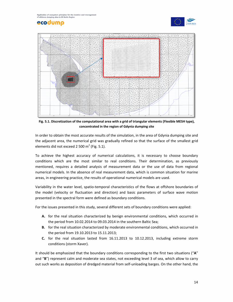
Fig. 5.1. Discretization of the computational area with a grid of triangular elements (Flexible MESH type),

concentrated in the region of Gdynia dumping site

In order to obtain the most accurate results of the simulation, in the area of Gdynia dumping site and

the adjacent area, the numerical grid was gradually refined so that the surface of the smallest grid

elements did not exceed 2 500 m2 (Fig. 5.1).

To achieve the highest accuracy of numerical calculations, it is necessary to choose boundary

conditions which are the most similar to real conditions. Their determination, as previously

mentioned, requires a detailed analysis of measurement data or the use of data from regional

numerical models. In the absence of real measurement data, which is common situation for marine

areas, in engineering practice, the results of operational numerical models are used.

Variability in the water level, spatio‐temporal characteristics of the flows at offshore boundaries of

the model (velocity or fluctuation and direction) and basic parameters of surface wave motion

presented in the spectral form were defined as boundary conditions.

For the issues presented in this study, several different sets of boundary conditions were applied:

A. for the real situation characterized by benign environmental conditions, which occurred in

the period from 10.02.2014 to 09.03.2014 in the southern Baltic Sea;

B. for the real situation characterized by moderate environmental conditions, which occurred in

the period from 19.10.2013 to 15.11.2013;

C. for the real situation lasted from 16.11.2013 to 10.12.2013, including extreme storm

conditions (storm Xaver).

It should be emphasized that the boundary conditions corresponding to the first two situations (“A”

and “B”) represent calm and moderate sea states, not exceeding level 3 of sea, which allow to carry

out such works as deposition of dredged material from self‐unloading barges. On the other hand, the

15

third situation (“C”), concerning much more dynamic environmental conditions, was selected to

evaluate the intensity of resuspension of previously deposited sediments.

For example, for the A‐situation, boundary condition related to variability in the water level and

parameters characterizing the wave spectrum at the northern boundary (offshore) of the model has

been shown in Fig. 5.3. Boundary condition in the MIKE model as a time series of relative changes in

sea water level [m], significant wave height [m], wave period [s] and direction of wave propagation

[0] (arrows)Fig. 5.2.

Fig. 5.3. Boundary condition in the MIKE model as a time series of relative changes in sea water level [m], significant wave height [m], wave period [s] and direction of wave propagation [0] (arrows)Fig. 5.2.

Similarly, for the B‐situation, boundary condition related to variability in the water level and

parameters characterizing the wave spectrum at the northern boundary of the model has been

shown in Fig. 5.4. Boundary condition in the MIKE model as a time series of relative changes in sea

water level [m], significant wave height [m], wave period [s] and direction of wave propagation [0]

(arrows)Fig. 5.3.

16

Fig. 5.4. Boundary condition in the MIKE model as a time series of relative changes in sea water level [m], significant wave height [m], wave period [s] and direction of wave propagation [0] (arrows)Fig. 5.3.

Boundary condition concerning a time series of water level variability and parameters characterizing

the wave spectrum at the northern boundary of the MIKE model for the most dynamic C‐situation

has been presented in Fig. 5.5. Boundary condition in the MIKE model as a time series of relative changes

in sea water level [m], significant wave height [m], wave period [s] and direction of wave propagation [0]

(arrows)

Fig. 5.5. Boundary condition in the MIKE model as a time series of relative changes in sea water level [m],

significant wave height [m], wave period [s] and direction of wave propagation [0] (arrows)

17

5.3 Initial conditions

An initial condition determines the physical state of a mathematical model at the moment (t0) of

starting numerical simulation.

For the issues described in this study, the initial conditions are as follows:

in the hydrodynamic module (HD): spatial distribution of sea water levels, distribution of velocities for current field,

in the spectral wave module (SW): spatial distribution of waves,

in the mud transport module (MT): concentration of different fractions of suspended sediments, thickness of all the mobile sediment layers.

In the implemented simulations, water level value at the time t0 for the entire water body

corresponds to the water level value of the boundary condition at the analogous point in time, and

surface waves are not taken into account. Additionally, concentration of different fractions of

suspended sediments, as an unknown value in the investigated water body, was set at zero level

(implementation of the excess‐type issue).

5.4 Environmental forcings

The environmental forcings in the conducted numerical simulations are: sea waves, sea currents,

variability in the water level, as well as the effect of wind over the water body, which, as a result of

the sheer stress, transfers the energy affecting wave motion and current variability. While the first

three factors, mentioned above, are imposed in the boundary conditions of specific model

configurations, the last condition is defined as variable in time and standardized for the entire study

area. Depending on the adopted computational scenarios, it is assumed to be a "real" distribution of

two‐dimensional variable (wind speed and direction) – the result of the atmospheric regional‐scale

model HIRLAM.

Wind forcings applied in the presented calculations have been shown in Fig. 5.4. Real forcing

condition in the MIKE model as a time series of changes in wind speed [m/s] and wind direction , Fig.

5.5, Fig. 5.6Error! Reference source not found. which correspond to the situations described above:

“A”, “B” and “C”.

18

Fig. 5.4. Real forcing condition in the MIKE model as a time series of changes in wind speed [m/s] and wind direction

Fig. 5.5. Real forcing condition in the MIKE model as a time series of changes in wind speed [m/s] and wind

direction

19

Fig. 5.6. Forcing condition as a scenario in the MIKE model – a time series of changes in wind speed [m/s] and

wind direction

It should be noted that works connected with dredged material disposal from self‐unloading dump

scows and with embedding power cables or pipelines are conducted when a sea state do not restrict

the vessel’s ability to operate. Thus, the application of environmental forcings at low or moderate

levels is most correct.

5.5 Scenarios

Dredged material deposition

Dredging works are carried out under favorable environmental conditions: weak waves and calm or

moderate wind conditions. The issue of dredged material deposition was analyzed assuming “A” and

“B” boundary conditions presented in section 5.2, and under appropriate wind forcing characterized

in section 5.4. In the study periods, different direction of winds occurred and it was included in the

analysis of suspended sediment dispersion.

The adopted scenarios were based on mathematical modeling of processes that are close to those

occurring during actually performed dredging works.

Multi‐bucket or single‐bucket dredgers, similarly as in the case of the port in Gdynia, deepen harbor

basins and load dredged material onto dump scows. In the scenario, self‐propelled and split hull

dump scows were used, in order to allow for self‐unloading. The carrying capacity of SM660 dump

scow is 660 m3. The analysis of scow operating time enabled to determine the period of time

between subsequent discharges of dredged material on the dumping site. In the model scenario, it

was assumed that dredged material is unloaded four times a day for the following 25 days and the

time of unloading is 3 min. Each time, dredged material discharged from a dump scow consisted of:

lumps of cohesive sediment, fine‐grained sand, mixture of silts, clays and water. For the purpose of

numerical modeling, it was assumed that one half of the load was fine sand and the other half was

mostly silty material. Only about 3% of sand fraction goes into suspension, while in case of silt

fraction with high water content, the amount which can be suspended is much higher, reaching up to

35%. The information concerning dredged material and dredging machinery/equipment was

obtained from the Port of Gdynia. The most important, from the point of view of numerical

20

modeling, are the particles of diameters smaller than 0.063 mm, which go into suspension and

remain as suspended particles for a period from several to several tens hours. Non‐cohesive

sediments and lumps of cohesive compacted solids reach the bottom after a short time and remain

there. Time, place and load of every single discharge are assumed within each computational

scenario. Dredged material (divided into fractions) is defined by parameters characterizing its

behavior in the water column, such as: fall velocity, limiting concentrations for the flocculation

process or initiation of hindered settling, dispersion and critical shear stress, below which deposition

occurs. Furthermore, the parameters such as: bottom roughness, density of different sediment

layers, critical shear stress for resuspension process in different bottom layers, are defined. Gdynia

dumping site can be characterized by relatively large water depths in the range of 27‐52 m. For

modeling dredged material discharges of small volume, morphological changes, having a negligible

effect on flow hydrodynamics, were not taken into account in the scenarios.

Resuspension process

Resuspension of sediments can occur only in the environmental conditions described as storm

conditions. These conditions exceed acceptable limits for using dredging equipment. As a result, in

order to consider the process of resuspension, the following scenario has been proposed:

environmental forcings described in the situation “B” are appropriate to conduct disposal operations,

and extreme forcings, described in the situation “C” occur immediately after the disposal and can

potentially cause resuspension process. The boundary conditions for this scenario have been

presented in the description of “C” situation in section 5.2.

It has been assumed that immediately after the deposition of dredged material, the surface layer of

the seabed within the area of the dumping site is partially covered with new sediments and the

conditions for resuspension of these particles have been characterized in section 3.

Forcing conditions in the scenario prepared to analyze the process of resuspension are the conditions

adopted from the real storm Xaver, which probability of occurring is lower than once in 50 years.

6. Verification of data sources for boundary conditions

Due to the lack of measurement data, for the local MIKE model, it was decided to use boundary

conditions and environmental forcings taken from the regional‐scale models (e.g. HIROMB, WAM).

In order to verify this approach, the results of the regional models were compared with

measurements conducted at hydrological coastal stations and with the results from the measuring

instrument installed in the area used for model computations.

6.1 Sea level variations

Temporal variability of sea water levels [cm] in the period from 01.09. 2013 to 31.10.2013 was

analyzed at 5 coastal water gauge stations (Vistula River Mouth, Northern Port of Gdańsk, Gdynia,

Puck, Hel). The results from observations at these stations comply with one another very well (Fig.

6.1. Changes in sea water level [cm], from 2013.09.01 to 2013.10.31, at 5 coastal water gauge stations

(Vistula River Mouth, Northern Port of Gdańsk, Gdynia, Puck, Hel) ). It is reflected by high values of linear

correlation coefficients (r> 0.9), which are a measure of linear, statistical relationship between two

21

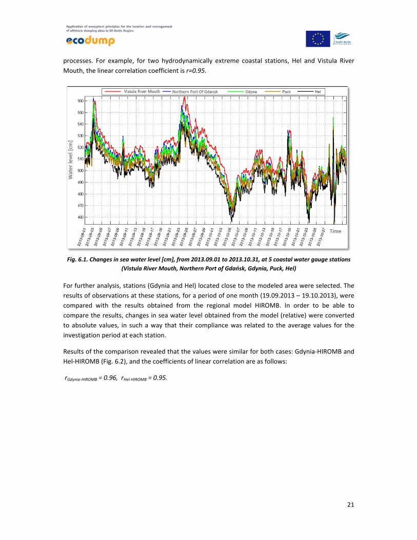
processes. For example, for two hydrodynamically extreme coastal stations, Hel and Vistula River

Mouth, the linear correlation coefficient is r=0.95.

Fig. 6.1. Changes in sea water level [cm], from 2013.09.01 to 2013.10.31, at 5 coastal water gauge stations

(Vistula River Mouth, Northern Port of Gdańsk, Gdynia, Puck, Hel)

For further analysis, stations (Gdynia and Hel) located close to the modeled area were selected. The

results of observations at these stations, for a period of one month (19.09.2013 – 19.10.2013), were

compared with the results obtained from the regional model HIROMB. In order to be able to

compare the results, changes in sea water level obtained from the model (relative) were converted

to absolute values, in such a way that their compliance was related to the average values for the

investigation period at each station.

Results of the comparison revealed that the values were similar for both cases: Gdynia‐HIROMB and

Hel‐HIROMB (Fig. 6.2), and the coefficients of linear correlation are as follows:

rGdynia‐HIROMB = 0.96, rHel‐HIROMB = 0.95.

22

Fig. 6.2. Comparison of changes in the water level [cm] at the water gauge stations Gdynia (top) and Hel

(bottom) with data obtained from the HIROMB model

Due to the fact that the offshore boundary of the local‐scale numerical model MIKE is considerably

far from the shoreline (Fig. 5.2, section Error! Reference source not found.), it is necessary to choose

the correct boundary condition for sea water changes.

The above analysis, which confirmed high compliance of sea level changes from the HIROMB model

and data obtained from the measurements at coastal stations (Gdynia, Hel), justifies the acceptance

of data from the regional HIROMB model for further numerical computations in the MIKE model.

6.2 Wave parameters

Measurement data from the selected point within Gdynia dumping site were obtained based on the

registration of current velocities and wave heights by an acoustic current profiler of AWAC‐type

(Acoustic Wave And Current) set at that point (location of the instrument has been presented in

Fig. 6.3).

23

Fig. 6.3. Location of an AWAC instrument (λ=18.690661°, ϕ=54.549538°)

The results of significant wave heights Hs [m] obtained from the measurements by AWAC, for a

period of two months (19.10.2013 – 19.12.2013), were compared with the results obtained from the

regional WAM model (WAM grid point closest to the dumping site). Comparison of time series

variation in Hs from measurements and from the model has been shown in Fig. 6.4.

Fig. 6.4. Comparison of significant wave height Hs [m] time changes measured with the AWAC and

obtained from the regional WAM model

The graph shows high compatibility of two series of data, and the linear correlation coefficient is r =

0.92.

24

This analysis also confirms high compliance of the results of significant wave height changes from the

WAM model with observational data from AWAC instrument, which justifies the acceptance of data

from the regional model WAM for further numerical computations in the MIKE model. Similarly, the

results of wave period Tp [s] measurements with an AWAC (19.10.2013 – 19.12.2013) were compared

with the results obtained from the regional WAM model. The comparison of time series

variations in Tp, from the measurements and from the model, has been presented in Fig. 6.5.

Fig. 6.5. Comparison of wave period Tp [s] time changes measured by AWAC and obtained from the

regional WAM model

The graph shows high compatibility of two data series, and the linear correlation coefficient r equals

0.50.

7. Numerical model validation

After numerical simulations conducted with the use of the local‐scale MIKE model (in which data

from regional models HIROMB and WAM were used as boundary conditions and forcing), the results

were compared with the real data obtained from measurements at the selected point within the

dumping site. The purpose of this comparison was to calibrate the hydrodynamic model, based on

measurement data. The following figures show the results of the comparison of data from numerical

computations after the model calibration process, and measurement data collected by AWAC

instrument.

Error! Reference source not found. presents a time series of changes in sea water level, while in Fig.

7.2 we can see the comparison of the variation in time of significant wave height Hs.

Fig. 7.3 shows the comparison of sea current velocities at the same point.

A good agreement of the measurement data with the results of computations was observed for sea

water levels, wave heights and current velocities.

25

Calibration of the hydrodynamic model included changes in the bottom roughness and

characteristics of wind friction. The application of appropriate changes led to the improvement in the

agreement between calculated and measured sea currents.

Fig. 7.1. Comparison of sea level changes in time (2013.09.19‐2013.10‐29) between the results from the MIKE

and HIROMB models and data measured by AWAC in the chosen point within the dumping site

Fig. 7.2. Comparison of significant wave height changes in time (2013.11.16‐2013.12.10) between the results

from the MIKE models and data measured by AWAC in the chosen point within the dumping site

Fig. 7.3. Comparison of current velocity changes in time (2013.11.16‐2013.12.10) between the results from

the MIKE models and data measured by AWAC in the chosen point within the dumping site

8. Calculation results

8.1 Scenario – dredged material deposition – case study “A”

26

The results of simulation concerning the dumping of dredged material have been presented for the

subsequent time steps (t1, t2, t3, t4, t5) in the figures

, Error! Reference source not found., Error! Reference source not found.,

and Fig. 8.5, in the following way:

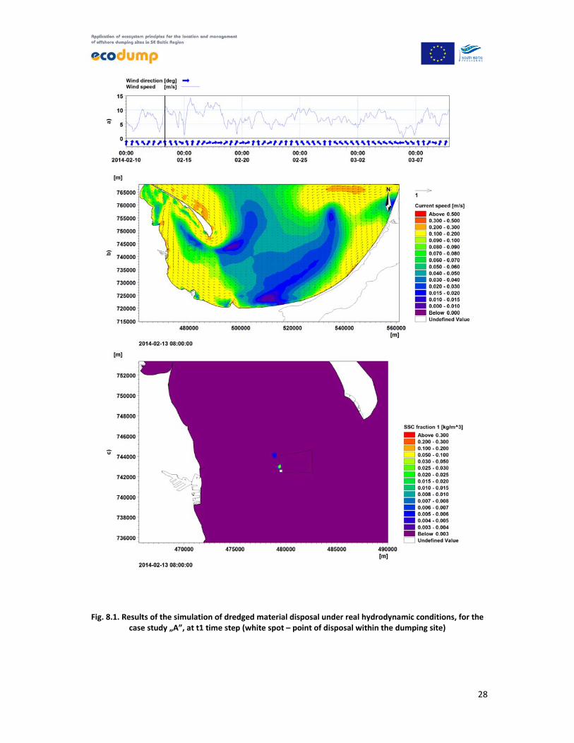
a) graphs of wind speed and direction variability in time, over the basin (black vertical line

represents the moment of simulation shown on the maps of currents, waves and

concentrations),

b) map of current circulation in the Gulf of Gdańsk (directions and averaged velocities),

c) map of suspended sediment dispersion in the zoomed area including Gdynia dumping site

(concentration of suspended solids in kg/m3, which is equal to g/l), and:

d) in the case of the last figure (Fig. 8.4) – map of changes at the sea bottom within the area of

Gdynia dumping site after disposal works,

where the subsequent time steps mean:

t1 – moment in time 2 hours after the discharge under the prevailing wind from the south (

),

t2 – moment in time 2 hours after the discharge under the prevailing wind from the west

(Error! Reference source not found.),

t3 – moment in time 2 hours after the discharge under the prevailing wind from the east

(Error! Reference source not found.3),

t4 – moment in time when the spatial impact of suspended sediments is the greatest (Error!

Reference source not found.4),

t5 – moment in time when all the disposal operations have been finished (

5).

Each set of pictures shows the simulation at subsequent time steps of the adopted calculation

scenario.

At t1 time step, the maximum extent of spreading of the sediment plume is moderate and it reaches

a distance of approx. 2.8 km from the point of discharge, with an average concentration decreasing

quickly. After 2 hours, the maximum concentration in the center of the plume located close to the

point of discharge is 60 mg/l. However, in the second plume, approx. 1.1 km away from the point of

discharge, after 8 hours from the time of discharge, the concentration is very low and does not

exceed 6 mg/l. During this period, the wind from the south has been blowing over the basin area for

a period more than ten hours. Maximum speeds of the current within the dumping site are small

(0.06 – 0.08 m/s). The dumping site is in the area of current circulation, and as a result, the

suspended sediments disperse in a north‐westerly direction.

27

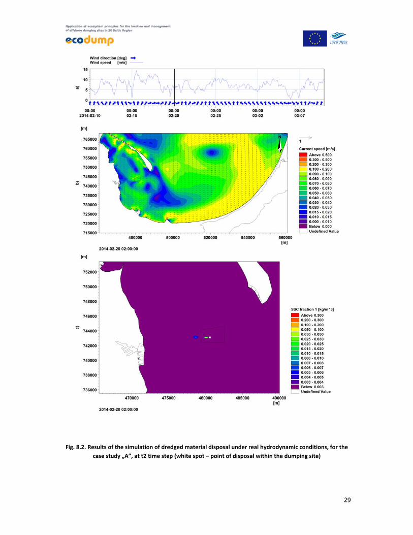
At t2 time step, the maximum extent of spreading of the sediment plume reaches about 3.2 km from

the point of discharge. The concentration of suspended solids decreases rapidly. After 2 hours, the

maximum concentration in the center of the plume located close to the point of discharge is 55 mg/l.

In the second plume, which is approx. 1.5 km away from the point of discharge, after 8 hours the

concentration is low and it equals 7 mg/l. During this period, the wind over the basin has been

blowing from the west for over ten hours, at a speed not exceeding 7 m/s. Maximum speeds of the

current within the dumping site, for such forcing, are in the range of 0.06 – 0.09 m/s. The generated

current circulation causes that the plume is moving in a westerly direction, i.e. in the direction

opposite to the direction of the wind.

At t3 time step, the maximum extent of spreading of the sediment plume reaches 1.8 km from the

point of discharge. The concentration of suspended solids decreases rapidly. After 2 hours from the

time of discharge, the maximum concentration in the center of the plume is 20 mg/l. The plume

disappears after 6 hours from the time of discharge. During this period, the wind over the basin

changes from a south‐eastern to eastern direction and its speed decreases from 9 to 5 m/s.

Maximum speeds of the current within the dumping site for such forcing reach up to 0.2 m/s, and the

direction in which the sediment plume is moving is similar to the direction of the wind.

At t4 time step, the spatial area of the plume reaches the maximum size for the entire simulation.

The length of the plume is 3.5 km and the maximum width equals 0.6 km. The maximum

concentration reaches 67 mg/l. Such situation occured when the southern wind increased.

Suspended solids are present at elevated concentrations due to low current velocity.

At t5 time step, the state of the bottom after disposal and sedimentation of dredged material has

been presented (all the sites of disposal can be easily seen there). A newly formed layer of

sediments, locally in the areas of the disposal, has a thickness of up to 0.33 m. The analysis of

sediment thickness after finishing the disposal works indicates that sediments formed from the

suspension outside the area of the dumping site are negligible and their thickness in the modeling

does not exceed 2 mm.

28

Fig. 8.1. Results of the simulation of dredged material disposal under real hydrodynamic conditions, for the case study „A”, at t1 time step (white spot – point of disposal within the dumping site)

29

Fig. 8.2. Results of the simulation of dredged material disposal under real hydrodynamic conditions, for the

case study „A”, at t2 time step (white spot – point of disposal within the dumping site)

30


case study „A”, at t3 time step (white spot – point of disposal within the dumping site)

31

Fig. 8.4. Results of the simulation of dredged material disposal under real hydrodynamic conditions, for the case study „A”, at t4 time step (white spot – point of disposal within the dumping site)

32

Fig. 8.5. Results of the simulation of dredged material disposal under real hydrodynamic conditions, for the case study „A”, at t1 time step

33

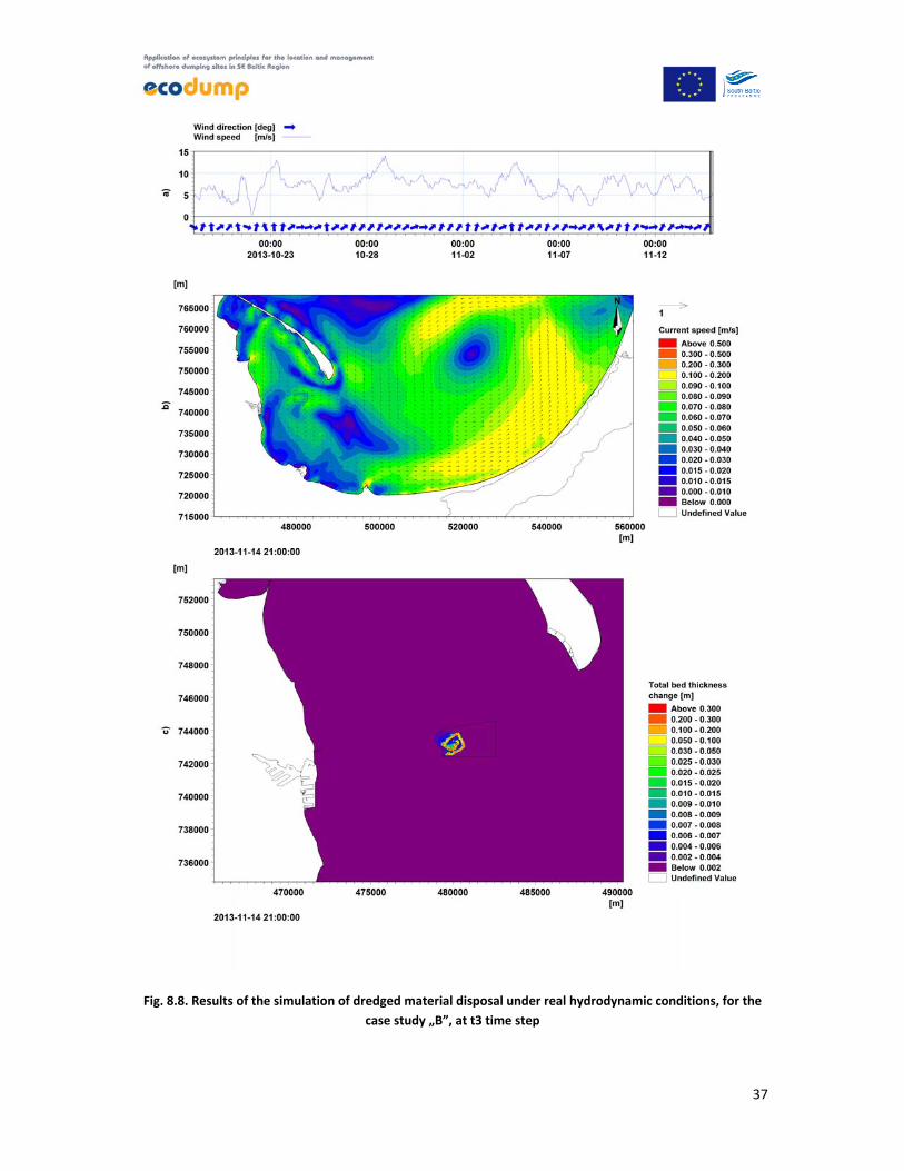
8.2 Scenario – dredged material deposition – case study “B”

The results of simulation concerning the discharge of dredged material have been presented for the

subsequent time steps (t1, t2, t3) in the figures Error! Reference source not found., Error! Reference

source not found., Error! Reference source not found., in the following way:



concentrations),



(concentration of suspended solids in kg/m3, which is equal to g/l), and

d) in the case of the last figure (Error! Reference source not found.) – map of changes at the

sea bottom within the area of Gdynia dumping site after disposal works,


t1 – moment in time 2 hours after the discharge under the prevailing wind from the south‐

west (Error! Reference source not found.6),

t2 – moment in time 2 hours after the discharge under the prevailing wind from the west

(Error! Reference source not found.7),

t3 – moment in time when all the disposal operations have been finished (Error! Reference

source not found.).


scenario.

At t1 time step, the maximum extent of spreading of the sediment plume is minor and it reaches a

distance of approx. 1.4 km from the point of discharge, with an average concentration decreasing

quickly. After 2 hours, the maximum concentration in the center of the plume located closer to the

point of discharge is 30 mg/l. However, in the second plume, approx. 1.3 km away from the point of

discharge, after 8 hours from the time of discharge, the concentration is very low and does not

exceed 4 mg/l. During this period, the wind from the south‐west has been blowing in the basin area

for over ten hours. Maximum velocities of the current within the dumping site are small (0.06 – 0.09

m/s). The sediment plume is moving in a north‐westerly direction i.e., rotated 90o in relation to the

wind direction.

At t2 time step, the maximum extent of spreading of the sediment plume reaches about 2.4 km from

the point of discharge. The concentration of suspended solids decreases rapidly. After 2 hours, the

maximum concentration in the center of the plume located closer to the point of discharge is 47

mg/l. In the second plume, which is approx. 2.2 km away from the point of discharge, after 8 hours

the concentration is low and it equals 4 mg/l. During this period, the wind over the basin has been

blowing from the west for over ten hours, at a speed not exceeding 9 m/s. Maximum velocities of the

current within the dumping site, for such forcing, are in the range of 0.06 – 0.09 m/s. The generated

34

current circulation causes that the plume is moving in a westerly direction, i.e. similarly as in the case

study “A” – in the direction opposite to the direction of the wind.

At t3 time step, the state of the bottom after disposal and sedimentation of dredged material has

been presented. A newly formed layer of sediments, locally in the areas of disposal, has a thickness

of up to 0.38 m. The analysis of sediment thickness after finishing the disposal works indicates that,

similarly as in the case study “A”, thickness of sediments formed from the suspension outside the

area of the dumping site is negligible.

35


case study „B”, at t1 time step (white spot – point of disposal within the dumping site)

36


case study „B”, at t2 time step (white spot – point of disposal within the dumping site)

37


case study „B”, at t3 time step

38

8.3 Scenario – resuspension process – case study “C”

In this section, the results of simulations concerning the fate of dredged material deposited on the

dumping site and subjected to the influence of waves and currents during the extreme storm have

been presented. This scenario is related to the process of resuspension of sediments deposited at

Gdynia dumping site. The results which are typical for the case of significantly increased dynamics of

forcing conditions in the model have been shown for the subsequent time steps (t1, t2, t3) in the

figures Error! Reference source not found., Error! Reference source not found., Error! Reference

source not found., in the following way:



concentrations),



(concentration of suspended solids in kg/m3, which is equal to g/l),


t1 – moment in time when resuspension has started (Error! Reference source not found.),

t2 – moment in time when the greatest concentration in the plume can be observed (Error!

Reference source not found.),

t3 – moment in time which reflects the extent of spreading of the sediment plume (Error!

Reference source not found.).


scenario.

At t1 time step, the process of resuspension begins. Significant wave heights in the area of Gdynia

dumping site reach up to 1.2 m, however, taking into account water depths at this site (25‐55 m), the

impact of the oscillating motion generated by waves on sediments is negligible. Average

concentrations of the turbidity plume which starts forming are very low. At the initial t1 moment

they reach approx. 4 mg/l.

After 4 hours, at t2 time step, the size of the plume reaches its maximum (length: m, width: m) and

the average concentration of suspended sediments ranges from 4 to 6 mg/l. In this period, the wind

blows from the west and reaches speeds of 18 m/s. The location of Gdynia dumping site causes that

the strongest storm induced by NW winds cannot generate considerably high waves in this area.

At t3 time step, after next 5 hours, the plume disappears, its concentration is decreasing and reaches

<3 mg/l after traveling a distance of approx. 5 km from the place of appearance.

39

Fig. 8.9. Results of the simulation of dredged material disposal and the effect of resuspension under real

hydrodynamic conditions, for the case study „C”, at t1 time step

40

Fig. 8.10. Results of the simulation of dredged material disposal and the effect of resuspension under real

hydrodynamic conditions, for the case study „C”, at t2 time step

41

Fig. 8.11. Results of the simulation of dredged material disposal and the effect of resuspension under real hydrodynamic conditions, for the case study „C”, at t3 time step

42

9. Summary The objective of this study (task within the ECODUMP project) was to build a numerical model which

in the most reliable way could predict the dispersion of suspended sediments, both in terms of space

and time. For this study it has been tested in the area of Gdynia dumping site. The key issue in this

type of computations is to quantitatively assess the concentration of suspended material during and

after deposition of dredged material.

The results of all the calculations lead to the following general conclusions:

Complex numerical models like MIKE21 allow for a more realistic approach to dumping and

resuspension processes.

Numerical models require validation against the measurements, as long as the gaps in the

knowledge still exist.

The agreement of real‐scale measured data with the regional models (WAM, HIROMB) and

the local model (MIKE21) are fully satisfactory in terms of wave parameters and sea level

fluctuations.

Over ten various computational scenarios were performed as part of the task and three of them

were selected to be presented in this study. The scenarios differed primarily in the directions and

intensity of environmental forcings.

The analyses of the dispersion of suspended sediments during the discharge of dredged material

were modeled for calm and moderate wind conditions – the actual conditions in which disposal

works are carried out. In the case of works connected with deposition of dredged material, not only

the process of dispersion of suspended sediments during the dumping is analyzed but also the

resuspension of deposited sediments caused by hydrodynamic forces being the result of extreme

meteorological and hydrological impacts.

Within the task, as part of the ECODUMP project, several measurement sessions were carried out at

the site in the area of Gdynia dumping site using AWAC instrument – Acoustic Wave And Current

Profiler. The results of the measurements were used for the calibration of the model and to prove its

usefulness. The application of the numerical model for the analysis of Gdynia dumping site, located in

the Gulf of Gdańsk, leads to the following specific conclusions:

The biggest differences in the calculated current velocity fields occur in the case of

environmental forcings (from the NW‐NE sector) which are influenced by complicated

configuration of the shoreline. For such conditions, an important role is played by currents

generated inside the Bay of Puck, as well as the currents coming from an open area of the

Gulf of Gdańsk, causing the appearance of specific current circulation systems.

The results of calculations in the modeling scenarios for environmental forcings from E to SW

directions indicate a much better agreement of the current‐related parameters between

measurement and simulation data.

The occurrence of complex current circulations, especially in confined water bodies, can lead

(as shown in the results of computations) to situations in which spreading of the sediment

plume takes place in a direction considerably different from the direction of the blowing

43

wind or even opposite to it. In such case, an increase in the wind speed not always leads to

an increase in the extent of the sediment plume.

In the case of weak winds, the concentration of suspended sediments after the dumping of

dredged material reaches higher values and the impact period of the plume can be longer.

At the time of dredged material discharge, concentrations of suspended solids, especially

when fine fractions are predominant, reach significant values. However, they rapidly

decrease. In the analyzed cases of disposal from dump scows, which are very popular in

Gdynia, average concentrations of the sediment plume outside the dumping site are very

low.

Unloading of a single dump scow (see section 5.5) creates a new layer of sediments at the

bottom, which has a thickness not exceeding 0.4 m, for water depths of Gdynia dumping site.

The location of Gdynia dumping site causes that resuspension can occur only in the case of extreme

storms. It results from the fact that the basin is surrounded by land on three sides and, additionally, it

has considerable water depths in the area of the dumping site.

References

1. Burcharth F.H., Hawkins S.J., Zanuttigh B., Lamberti A., (2007). Environmental Design Guidelines

for Low Crested Coastal Structures. Elsevier, The Netherlands.

2. Cieślikiewicz W., Paplińska‐Swerpel B., (2005). Long‐term modeling of wind waves in the Baltic

Sea, in the period 1958‐2001 (in Polish). Inżynieria Morska I Geotechnika, No. 4, 313‐321.

3. Dembska G., …. (2014). Report on quantity, types and characteristics of the sediments from

existing dumping sites in SE Baltic. ECODUMP Project, Gdańsk.

4. Gűnter H., (2002). WAM Cycle 4.5 User Manual. Institute for Coastal Research, Hamburg.

5. Hornsea Offshore Wind Farm (2013). Project One. Annex 5.1.6. Cable Burial Plume Assessment.

6. Komen, G.J., Cavaleri L., Donelan M., Hasselmann K., Hasselmann S. and P.A.E.M. Janssen,

(1994). Dynamics and modelling of ocean waves. Cambridge University Press, Cambridge.

7. MIKE 21/3 Coupled Model FM, User Guides, (2008). DHI Software.

8. MIKE 21 Wave Modelling, (2007). Vol. 1, DHI Software.

9. MIKE 21 Flow Model FM, Hydrodynamic Module, User Guide, (2013). DHI Software.

10. MIKE 21 Flow Model FM, Mud Transport Module User Guide, (2013). DHI Software.

11. Paplińska B., (1999). Wave analysis at Lubiatowo and in the Pomeranian Bay based on

measurements from 1997/1998 – comparison with modelled data (WAM4 model). Oceanologia,

41(2), 241–254.

12. Van Leussenm W. (1988). Aggregation of particles, setteling velocity of mud flocs. Areview: In:

Dronkers And Van Leussen (Eds.): Physical processes in estuaries. Springer Verlag. Pp 347‐403.

13. Van Rijn, L.C., (1993). Principles of sediment transport in rivers, estuaries and coastal seas. Aqua

Publications, The Netherlands.

Date post:	26-Aug-2018
Category:	Documents
Upload:	ngonhi
View:	218 times
Download:	0 times

Pilot study Gdynia – Numerical modelling -...

Documents