1

Pilot-wave quantum theoryin discrete space and time

and the principle of least actionJanusz Gluza, Institute of Physics, University of Silesia,

Uniwersytecka 4, PL-40-007 Katowice, Poland,Email: janusz.gluza@us.edu.pl

Jerzy Kosek, Institute of Physics, University of Silesia,Uniwersytecka 4, PL-40-007 Katowice, Poland,

Email: jkosek@us.edu.plJune 10, 2016

Abstract—The idea of obtaining a pilot-wave quantum theoryon a lattice with discrete time is presented. The motion ofquantum particles is described by a |Ψ|2-distributed Markovchain. Stochastic matrices of the process are found by the discreteversion of the least-action principle. Probability currents are theconsequence of Hamilton’s principle and the stochasticity of theMarkov process is minimized. As an example, stochastic motionof single particles in a double-slit experiment is examined.

I. INTRODUCTION

In classical physics the motion of a system of particlescan be elegantly described by Hamilton’s principle of leastaction. It states that for given initial and final space-timeconfigurations the real path of the system is the one for whichan action takes a stationary value. In quantum mechanicsformulated by Heisenberg in 1925 and by Schrodinger in 1926,the situation is different. It describes time evolution of thewave function (in the Schrodinger picture), while the classicalnotion of a sharp trajectory followed by a physical system isrejected. One of the alternatives is a pilot-wave formulationof quantum mechanics proposed by de Broglie in 1927 [1],and re-discovered by Bohm in 1952 [2], where particles havedefinite positions during their motion, similarly as in classicalmechanics. This idea was later extended to quantum fieldtheories (QFT), both bosonic and fermionic. In particular,some Bell-type QFTs describe creation and annihilation ofparticles, which, in addition, follow real trajectories [3], [4],[5], [6]. These models deal with continuous space-time, andgeneralize a lattice quantum field theory proposed by Bell [7],where the latter is based on specific choices of probabilitycurrents and jump rates.

Despite these prominent achievements there are severalmotivations for developing an analogical approach to quantum(field) theory in discrete space-time. First, space-time is treatedas continuous both by classical and standard quantum physics.However, one cannot exclude discrete space-time hypothesis.The situation can be similar to the discovery of a discretenature of such fundamental quantities as quanta of energy,charge or angular momentum, etc. Of particular importanceis the development of a quantum theory of gravity. Different

proposals based on the idea of discrete space-time weregiven (in particular, see [9], the proposal focused on loopquantum gravity, which poses elementary extensions of spaceas the primitive ontology of the theory). Also the notion ofa digital universe with discrete space-time is commonly usedand exploited now (see, e.g. [10]). Moreover, discrete space-time models are well suited for calculations, and de facto allcomputer calculations are discrete in nature.

A quantum model aimed to develop a Bell-type stochasticprocess on a lattice in discrete time was studied in [11]. It wasproven that a genuine analog of Bell’s process does not existin discrete time, however, proposals of processes that couldbe used as a replacement were given. The problem is that inthe discrete case there is not an obvious formula for the netprobability current between discrete states, such that it couldsubstitute the continuous case (see Eq. 6 below).

In this paper we present a new pilot-wave model on a latticeconfiguration space in discrete time. We take the positionsof the particles as the primary variables, similar to BohmianMechanics and Bell-type QFTs [5]. The theoretical schemepresented here is used to find stochastic paths for massiveparticles in quantum theory.

We do not assume any arbitrary formula for a probabilitycurrent. Rather, we describe the motion of quantum particlesby a |Ψ|2-distributed Markov chain, where stochastic matricesfor any two subsequent instants are found by Hamilton’sprinciple. Thus, probability currents are the consequence ofHamilton’s principle. We extend the principle to a latticeconfiguration space. It states that for given initial and finalquantum distributions—specified by a state vector Ψ—theaction averaged over a statistical ensemble of identical systemstakes a minimal value. This allows us to find unique stochasticmatrices of the process. Additionally, the stochasticity ofthe Markov process is minimized. In the case of singlenon-relativistic particles it means that their mean squaredisplacements over time are minimized.

Finally, Hamilton’s principle on a lattice with discrete timecan be viewed as an optimal transport problem, where anaverage action is equivalent to the so-called optimal transportcost. (For an introduction to the optimal transport, see [12],

arX

iv:1

606.

0288

3v1

[qu

ant-

ph]

9 J

un 2

016

2

[13]). We suppose that numerical methods developed in thefield of optimal transport could be used (or adopted) incomputation of quantum phenomena on a discrete space-timelattice.

The plan of this article is as follows. Section II brieflypresents Bohmian mechanics and some other pilot-wave mod-els with continuous time and continuous or discrete space,providing a theoretical background to the discrete space-time model. Section III defines stochastic matrices for aquantum system on a lattice configuration space. Section IVformulates the principle of least action on a lattice config-uration space in discrete time. Section V defines minimaltransition probabilities and proves it to be valid for our model.Section VI studies stochastic behavior of single massiveparticles. Section VII presents an example of double-slitexperiment with massive particles. Section VIII summarizesour results and gives concluding remarks. Appendix A presentsan algorithm for computing stochastic matrices with theminimal transition probabilities. Appendix B discusses thelink between Hamilton’s principle and the optimal transportproblem.

II. CONTINUOUS-TIME PILOT-WAVE MODELS

In Bohmian mechanics space-time is continuous, and thestate of the system at any time t is described by a configurationQ(t) = (Q1(t), ..,QN (t)) of N point particles moving in realspace R3. The wave function Ψt(q) given by the Schrodingerequation

i~∂Ψt(q)

∂t=(−

N∑k=1

~2

2mk∇2k + V (q)

)Ψt(q) (1)

plays the role of a guiding field for the particles; V : R3N → Ris the potential function; ∇k is the gradient relative to thespace coordinates of particle k, mk is its mass. The equationsof motion are

dQk

dt=

jkt (q)

|Ψt(q)|2∣∣∣q=Q(t)

, (2)

wherejkt (q) =

~mk

Im(Ψ∗t (q)∇kΨt(q)) (3)

is the usual quantum current. The system itself, dependingupon its initial position, follows a deterministic trajectory.

The guidance equation, Eq. 2, implies the property calledequivariance: a statistical ensemble of systems having adistribution in positions |Ψt0(q)|2 at t0 preserves the characterof this distribution at any later time t, i.e. the distributionis |Ψt(q)|2. As a consequence, predictions of Bohmian me-chanics are identical to the predictions of standard quantummechanics.

Other types of pilot-wave models are stochastic modelsinitiated by Nelson [14], [15]. Now, instead of Bohmianguidance equation one has a Langevin equation with stochasticparameters, while the wave function Ψ still satisfies theSchrodinger equation. Both de Broglie-Bohm and Nelson’smodels can be generalized in a way that the guidance equation,Eq. 2, is supplemented with additional terms [16], [17]. For

example, in the case of a single particle system a generalizedequation is [17]

dQ

dt=

jt(q) + jt(q)DG

|Ψt(q)|2+ α

~m

∇|Ψt(q)|2

|Ψt(q)|2+√αdω

dt

∣∣∣q=Q(t)

,

(4)where ∇· jt(q)DG = 0, α is a free parameter, and dω is aWiener process with dω = 0 and (dω)2 = ~/m.

An important feature is that the generalized guidanceequation, Eq. 4, gives rise to the same quantum distributions|Ψt(q)|2, and simultaneously the trajectories are different,depending on the choice of the parameters. For α 6= 0 weget stochastic theories, while for α = 0 deterministic ones.

So there is an infinity of possible wave-particle modelsin continuous space-time, both deterministic and stochastic.Bohmian mechanics is the one with the usual current j(jDG = 0) and no stochasticity (α = 0).

A. Discrete-space and continuous-time models

An extension of Bohmian mechanics into the discreteconfiguration space and continuous time is Bell’s model [7].It presents a Markov pure jump process (Qt)t∈R on a latticeconfiguration space Q. Bell aimed to reproduce the quantummechanical predictions for fermion number density in space.The same method—properly generalized—can be used tofind stochastic evolution for any discrete beables (i.e. thequantities supposed as objective elements of reality), both innon-relativistic quantum mechanics and in QFT. 1

Dynamics of the actual (field) configuration is stochastic—itis a consequence of the discretization of space. The transitionprobability from a configuration q to other configuration q′

(q′ 6= q) during a small interval dt is defined by Bell as

Pt(q → q′) =

{Jt(q

′, q)dt/Pt(q), Jt(q′, q) > 0,

0, Jt(q′, q) ≤ 0, (5)

where J stands for the probability current

Jt(q′, q) =

2

~Im[〈Ψt|P (q′)HP (q)|Ψt〉], (6)

Ψt is the state vector of a quantum (field) theory, evolvingin a Hilbert space H according to the Schrodinger equation;H is the Hamiltonian, P (q) is a projection to Hq ⊆H , andthe Hq form an orthogonal decomposition, H =

⊕q∈QHq;

Pt(q) is the probability distribution at time t

Pt(q) = 〈Ψt|P (q)|Ψt〉. (7)

The probability Pt(q → q) to stay in the same state q is

Pt(q → q) = 1−∑q′ 6=q

Pt(q → q′). (8)

Notice that the current J is defined in analogy to the currentj, Eq. 3. As it is antisymmetric, i.e., Jt(q, q′) = −Jt(q′, q),

1In Bell’s model, a continuous real space R3 is replaced by 3D spatial latticeΛ. At given time t, the actual configuration Q of fermion particles of the worldis one of the possible lists of integers q = (q1, . . . , qN ) ∈ Q, where N is themaximal index of the lattice sites, and qk are eigenvalues of fermion numberoperators acting at particular sites k of the lattice Λ (qk ∈ {1, 2, . . . , 4M},where M is the number of Dirac fields).

3

thus Eq. 5 implies Pt(q → q′) = 0 or Pt(q′ → q) = 0. So atleast one of transitions q → q′ or q′ → q is forbidden.

Solution Eq. 5 can be generalized [17], [18]. For example,one can add to Pt(q → q′) defined in Eq. 5 any solution P0

t

of the homogeneous equation

P0t (q → q′)Pt(q) = P0

t (q′ → q)Pt(q′). (9)

This generalization makes both of the transitions q → q′

and q′ → q possible. For all P0t (q → q′) = 0 one gets

Bell’s solution, Eq. 5, with minimal transition probabilities(or, equivalently, with minimal jump rates). This means thatat least one of the transitions q → q′ or q′ → q is forbidden.

III. STOCHASTIC MATRICES FOR QUANTUM SYSTEMS

In Sections III - VII we develop a new pilot-wave quantummodel on a lattice in discrete time. Basic assumptions ofthe model are as follows: We consider a system of Nstructureless and distinguishable particles and assume that allphysical beables are definite positions of the particles. Theconfiguration space Q is an ensemble of configurations ofdiscrete particle positions. The state of the system at time tis described by its actual configuration Qt = q ∈ Q. Thedynamics of the configuration is stochastic - it jumps from itsactual position at time t to another position Qt+τ = q′ ∈ Qat next time t+ τ , where τ is a discrete time step. Moreover,transition probabilities Pt(q → q′) ≡ P(Qt+τ = q′|Qt = q),depend only on the actual configuration Qt, and do not dependon the earlier states. This means that an evolution of the stateof the configuration is a Markov process (Qt)t∈τZ on Q withdiscrete time step τ .

Finally, we assume also that the transition probabilitiesdepend on the state vector Ψ which is the solution to theappropriate Schrodinger equation defined on Q

i~∂Ψu

∂u= HΨu, (10)

where u ∈ R is the continuous time parameter. Some discretevalues of u make discrete instants t, when stochastic jumpshappen (i.e., t = [u/τ ] ∈ τZ, where [x] means an integer partof x). 2

In the case of spinless particles we have an orthonormalbasis {|q〉 : q ∈ Q} of a Hilbert space labeled by Q.In general, the basis of a Hilbert space is indexed by theconfiguration q, as well as by additional quantum numbersm that are not related to beables, e.g. spin. Here we followBell who has shown in [19] that spinor-valued wave functionsfully account for all phenomena involving spin. The sametreatment of spin is in Bohmian Mechanics [20].3 In this waypositions can be the primary outputs of the theory, while otherquantities (momenta, energy, spin etc.) can be deduced fromthe positions.

2A similar assumption is presented in [11], where a Markov process indiscrete time is obtained by restriction to the integer times of Bell’s process(Qt)t∈R in continuous time.

3For example, the wave function of a spin-1/2 particle is a function Ψ :R3 → C2, and for N such particles it is a function Ψ : R3N → C2N .

Now, we define a stochastic matrix such that the quantumprobability distribution at time t

Pt(q) = 〈Ψt|P (q)|Ψt〉, (11)

is transformed into the probability distribution at time t+ τ

Pt+τ (q) = 〈Ψt+τ |P (q)|Ψt+τ 〉. (12)

P (q) =∑m |qm〉〈qm| is a projection. Namely, the stochastic

matrix Pt ≡ [Pt(q → q′)] includes probabilities of transitionsfrom q to q′, such that the following conditions are satisfied

Pt(q) =∑q′

Pt(q → q′)Pt(q), (13)

andPt+τ (q′) =

∑q

Pt(q → q′)Pt(q). (14)

These two equations express conservation of probability atparticular sites q ∈ Q at t and q′ ∈ Q at t+ τ , respectively.

The relations Eqs. 11 - 14 are general and do not definestochastic matrices uniquely. However, such matrices can bealways defined for any quantum system described by a wavefunction Ψt(q). One of the possible solutions is

Pt(q → q′) = 〈Ψt+τ |P (q′)|Ψt+τ 〉, (15)

which means that the transition probabilities depend only onthe wave function at latter time t + τ . In this solution theprobability is not locally conserved, but only on a global scale,as it involves jumps even from distant sites q to a given q′.

In general, there is a lot of freedom to find solutions forthis stochastic matrix, when the only requirement is that itrestores given probability distributions, Eqs. 11 and 12. Aunique solution locally conserving probability, based on theleast action principle, is proposed below.

IV. HAMILTON’S PRINCIPLE ON A LATTICE IN DISCRETETIME

Hamilton’s principle allows to formulate classical mechan-ics in a very general way. The formulation assumes continuousconfiguration space and continuous time. Now we adjust theprinciple to the discrete space-time case. It involves stochasticprocesses.

Let us consider a statistical ensemble of N identically pre-pared systems undergoing identical initial conditions, whichtake up sites q(ν) ∈ Q at time t, ν = 1, . . . ,N , and jump tosites q′(ν) ∈ Q at t+ τ .

We shall assume that the contribution from a single jumpfrom q(ν) to q′(ν) is the classical action, i.e., the time integralof the Lagrangian taken along the appropriate classical pathq(ν)(u), u ∈ 〈t, t+τ〉, as if the system really follows this path

St(q′(ν), q(ν)) = min

t+τ∫t

L(q(ν)(u), q(ν)(u)) du. (16)

Now, let us define a total action for the statistical ensemble

St(N ) =

N∑ν=1

St(q′(ν), q(ν)). (17)

4

In the lattice space Q the numbers St(q′(ν), q(ν)) belong tothe discrete set of actions calculated along all possible pathsconnecting sites q ∈ Qt and q′ ∈ Qt+τ , i.e. St(q′(ν), q(ν)) ∈{St(q′, q)}. Qt and Qt+τ are subspaces of Q such thatthe wave function is non-zero there at times t and t + τ ,respectively. Therefore, for Nt(q′, q) systems passing from qto q′ we can write

St(N ) =∑q′

∑q

Nt(q′, q)St(q′, q). (18)

In the limit N →∞ the quantity Nt(q′, q)/N approaches thetotal transition probability from q to q′, which is the transitionprobability Pt(q → q′) multiplied by the probability Pt(q)

limN→∞

Nt(q′, q)N

= Pt(q → q′)Pt(q). (19)

Thus, dividing Eq. 18 by N and taking a large N limit, weget an average value of the action

S(Pt) =∑q′

∑q

Pt(q → q′)Pt(q)St(q′, q), (20)

which depends on the choice of a stochastic matrix Pt. Now,Hamilton’s principle may be readily extended to define astochastic matrix for a Markov chain:

Among all possible stochastic matrices constrained byEqs. 11 - 14, a real Markov chain is defined by a matrixPt minimizing the average action

S(Pt) = min S. (21)

Constraints, Eqs. 11 - 12, depend on the wave function, sowe call them the quantum constraints (the other ones, Eqs. 13- 14, are also valid for classical stochastic matrices).

The description of the stochastic process will be completedby stating initial conditions. We assume that at some time t0the configuration Q(t0) is chosen randomly with probabilitydistribution |Ψt0(q)|2. The construction of the stochastic matri-ces guarantees that Q(t) has quantum distribution |Ψt(q)|2 atsubsequent times t ∈ τZ. Non-equilibrium initial distributionsare also valid (similarly as in other pilot-wave models, e.g. inBohmian-type quantum mechanics), and an open question ishow these distributions depend on time. However, we do notconsider this question in this paper.

In this way we have completed a definition of a Markovchain, where the only beables are particles’ positions. Itsproperties are studied in Sections V - VII.

V. MINIMAL TRANSITION PROBABILITIES

The stochastic quantum dynamics defined here imply va-lidity of the usual rules of probability, despite the fact thatspecific quantum phenomena are restored. For example, theprobability of finding a system at site qM at time tM isexpressed by a sum of total transition probabilities over all themutually exclusive alternative paths which start from positions

t

t

'a

a t b

'b

+C -C +C -C

t

Figure 1. A scheme of transformation which eliminates at least one ofsuperfluous transitions a → b′ or b → a′; C = min(Pt(b′, a),Pt(a′, b));Qt and Qt+τ are subspaces of Q such that Ψ is nonzero there at times tand t+ τ , respectively.

q0 at time t0 and follow positions q1, . . . , qM at t1, . . . , tM ,respectively:

PtM (qM ) =∑qM−1

. . .∑q0

PtM ,...,t0(qM , . . . , q0), (22)

and the multiplication rule is valid—as in any Markov process

PtM ,...,t0(qM , . . . , q0) =

M−1∏j=0

Pt(qj → qj+1)

Pt0(q0).

(23)On the other hand, counterintuitive quantum properties, as

an interference (see Section VII), an entanglement, etc., arenaturally embodied in the pilot-wave model.

A specific property of our model is that stochasticity of theMarkov process is minimized. An analogical property holdsin Bell-type models with continuous time [21]. As it was saidin Section II this entails that at least one of two transitionsq → q′ or q′ → q is forbidden. We will prove that an evenmore general property holds in our model. (Yet, we deal withdiscrete space-time.)

First, let us define as crossing transitions, a pair of transi-tions a→ b′ and b→ a′ such that

St(a′, a) < St(b

′, a) and St(b′, b) < St(a′, b), (24)

andPt(b′, a) 6= 0 and Pt(a′, b) 6= 0, (25)

where Pt(b′, a) = Pt(a → b′)Pt(a) and Pt(a′, b) = Pt(b →a′)Pt(b) are the total transition probabilities from a to b′ andfrom b to a′, respectively. Notice that in general a′ and b′ canbe different from a and b (see Fig. 1). It occurs that Hamilton’sprinciple eliminates at least one of two crossing transitions, i.e.a→ b′ or b→ a′ is forbidden, as

Pt(b′, a) = 0 or Pt(a′, b) = 0. (26)

To prove it we assume that proposition is not true, i.e.Pt(b′, a) 6= 0 and Pt(a′, b) 6= 0, while S(Pt) is minimal. Now

5

we define new total transition probabilities such that they donot change the probabilities at a, b, a′, and b′ (see Fig. 1), i.e.

Pt(a′, a) = Pt(a′, a) +C,

Pt(b′, b) = Pt(b′, b) +C,

Pt(b′, a) = Pt(b′, a) −C,Pt(a′, b) = Pt(a′, b) −C,

(27)

whereC = min(Pt(b′, a),Pt(a′, b)) (28)

(in general, C depends on a, b, a′, b′ and t). Eq. 27 impliesthat Pt(b′, a) = 0 or Pt(a′, b) = 0. However, the new valueS(Pt) is less than the old one S(Pt), because

S(Pt)−S(Pt) = C(St(a′, a)−St(b′, a)+St(b

′, b)−St(a′, b))(29)

is less than 0 (see Eq. 24). Thus we got a contradiction withthe assumption that S is minimal, q.e.d.

In particular, when a′ = a ≡ q and b′ = b ≡ q′ andEq. 24 holds (e.g. for a ”free” Lagrangian such as consideredin Section VI) one gets the characteristic feature of Bell-typemodels.

As a result, the crossing transitions are eliminated in thewhole net. In the case of single particles in flat space-timethis means that space-time trajectories cross themselves onlyin the space lattice nodes.

The non-crossing property is especially useful in the caseof 1D Markov process on a flat space. In that case it isequivalent to Hamilton’s principle, Eq. 21. Thus, searching fora minimum of the average action can be replaced by searchingfor non-crossing transitions, which is a simpler task allowingstochastic matrices to be calculated in an efficient way.

VI. STOCHASTICITY OF MOTION

Hamilton’s principle implies that the crossing transitionsin Q are eliminated. In consequence, the stochasticity of themotion in Q is minimized. Roughly speaking, it is becausewe get no more distant jumps than necessary for ensuring thequantum distributions.

To illustrate this, consider the motion of free single particles.We take Lorentz invariant action in Eq. 20 [22]

St(q′,q) = −mc2

t+τ∫t

√1− q2(u)/c2du (30)

where m is particle’s mass. In the non-relativistic limit we get

St(q′,q) = −mc2τ

(1− |q

′ − q|2

2c2τ2

). (31)

Now Eq. 20 reads

S(Pt) = K +m

2τ

∑q′

∑q

Pt(q→ q′)Pt(q) |q′ − q|2, (32)

whereK = −mc2τ (33)

and we have used∑q′

∑q

Pt(q→ q′)Pt(q) = 1. (34)

Constant numbers K and m/2τ can be omitted because theminimum of

S′(Pt) =∑q′

∑q

Pt(q→ q′)Pt(q) |q′ − q|2 (35)

leads to the same matrix elements Pt(q→ q′) as the minimumof S(Pt). The above formula can be written as

S′(Pt) =∑q

Pt(q)∆2t (q), (36)

where∆2t (q) =

∑q′

Pt(q→ q′) |q′ − q|2 (37)

is mean square displacement of particles moving from positionq at t to positions q′ at t + τ .4 The physical meaning ofHamilton’s principle is clear now: imposed on Eq. 36 theprinciple confines the motion of particles in a way that theirmean square displacements over time are minimized.

The total mean square displacement, Eq. 35, is equivalentto the average action in the non-relativistic limit, and thestochasticity of the motion can be measured by it. It is easy tosee that in a general case of more complex systems the averageaction S(Pt) can provide the measure of stochasticity.

VII. DOUBLE SLIT EXPERIMENT

As an example, we analyze typical double-slit interferenceof single particles, where a monochromatic plane incidentwave illuminates the diaphragm with two slits. Here weconsider spinless massive particles (let’s call them electrons).

A. An electron wave function

The wave function behind a single slit can be calculatedwith the aid of the Feynman path integrals [23]. Assumingpropagation of the wave with a constant speed vy along they-axis perpendicular to the diaphragm one has

Ψ(x, t) =

∫ a/2

−a/2K(x, t;x0, t0)Ψ(x0, t0)dx0, (38)

where Ψ(x0, t0) is the field on a slit, and

K(x, t;x0, t0) =

√m

2iπ~(t− t0)exp

(im(x− x0)2

2~(t− t0)

)(39)

is the propagator for a free particle of mass m. For aplane incident wave we have Ψ(x0, t0) = const. Substitutingt− t0 = y/vy into Eqs. 38 and 39 after some algebra we getthe wave function at point (x, y) behind the slit

Ψ(x, y) ∼ {C(u2)− C(u1) + i[S(u2)− S(u1)]}, (40)

where

u1(x, y) =

√2

λy

(x+

a

2

), u2(x, y) =

√2

λy

(x− a

2

),

(41)

4Eq. 37 can be expressed as the sum of the squared average distance ofjumps and variance of the positions q′ given q, i.e. ∆2

t (q) = (q−<q′>)2

+∑

q′ Pt(q→ q′) (q′−<q′>)2.

6

ix

kx

x

y j+1

jy

y

Figure 2. A scheme used in the calculation of trajectories: a particle jumpsfrom position q = (xi, yj) on line y = ∆y · j at time t to a positionq′ = (xk, yj+1) on line y = ∆y · (j + 1) at time t+ τ .

λ = h/mvy is de Broglie wavelength of the electron, and

C(u) =

u∫0

cos(π

2t2)dt, S(u) =

u∫0

sin(π

2t2)dt (42)

are the Fresnel integrals. In the case of two identical slits asuperposition of a suitably translated field of the single slit,Eq. 40, can be applied

Ψ(D)(x, y) = Ψ(x− d/2, y) + Ψ(x+ d/2, y), (43)

where d is the separation of the slits, (d/2, 0) and (−d/2, 0)are their centers.

Notice that the above equation should be regarded as anapproximation to the wave function for the lattice version ofthe Schrodinger equation, Eq. 10.

B. Simulation

The positions behind the diaphragm are restricted to thesites of a 2D regular lattice, xi = ∆x · i, i = 0, . . . , Nx, andyj = ∆y · j, j = 0, . . . , Ny . To simplify the calculation, weassume (see Fig. 2):

1) at time t the particle is at site q = (xi, yj) on the liney = ∆y · j parallel to the diaphragm, and

2) at time t+ τ it jumps randomly to site q′ = (xk, yj+1),xk = ∆x ·k, k = 0, . . . , Nx on the line y = ∆y ·(j+1);∆y = vy τ , where vy is the constant speed of the wavealong the y-axis.

Stochastic matrices Pt = [Pt((xi, yj)→ (xk, yj+1))] arecomputed as follows: First, the quantum distributions arecalculated Pt(xi, yj) = Ct|Ψ(xi, yj)|2, i = 0, . . . , Nx andPt+τ (xi, yj+1) = Ct+τ |Ψ(xk, yj+1)|2, k = 0, . . . , Nx, whereCt and Ct+τ are normalization constants dependent on ∆x.Then, to find the minimum of Eq. 35 the imposed (quantum)constraints, Eqs. 11 - 14, are taken into account. However, dueto computational reasons, directly searching for the minimumwould present a challenging task and an equivalent procedureis used based on the non-crossing property of transitions; thismade the calculation tractable (see Appendix A, where thealgorithm is presented).

-0.6 -0.4 -0.2 0 0.2 0.4 0.6

0

0.0025

0.005

0.0075

0.01

x [mm]

y [m

]

Figure 3. A net of possible transitions in a double slit experiment. Thewidth of the slits a = 0.1 mm, the distance between them d = 0.3mm. The wavelength λ = 700 nm. Colors indicate different ranges oftotal transition probabilities related to the maximal one in the net Pmax =0.016: gray [10−6, 10−3), olive [10−3, 10−2), sea green [10−2, 10−1),blue [10−1, 1].

A net of possible transitions (xi, yj)→ (xk, yj+1) behindthe diaphragm in the double slit experiment is shown in Fig.3. Zooming into a picture we explicitly checked that pathscrossed themselves only in the nodes of the net. This meansthat the stochastic matrix was really minimized.

The (computer) Monte Carlo algorithm to find the stochasticpaths is straightforward. It starts in a diaphragm, where aposition of a particle is chosen over the slit/slits width with auniform distribution (here it is an equilibrium distribution).Next, the procedure is repeated recursively, for a givenposition q = (xi, yj) a pseudo-random number is drawnand, depending on its value and the values of probabilitiesPt((xi, yj)→ (xk, yj+1)), k = 0, . . . , Nx, the particle jumpsto a new position q′ = (xk, yj+1).

In Fig. 4 the results are shown. We have taken λ = 700nm (equal to wavelength of an electron moving with speedv = 103m/s). The band at the bottom shows the distributionof particles on the final screen y = 0.1 m in the simulation,where 60 000 particles have been used. For clarity only 0.1%of the total number of trajectories is shown. Two shades ofblue are used to visualize individual trajectories in a betterway.

The picture reveals the interference phenomenon, and wehave checked that for an initial equilibrium distribution |Ψt0 |2it perfectly restored the equilibrium distributions |Ψt|2. Addi-tionally, the results tended to become closer to the theoreticaldistributions as more sampling particles were used, in agree-ment with the law of large numbers.

What we observe is that starting from the same initial state(source) and passing the diaphragm, particles move alongstochastic paths and reach a wide range of positions in the finalplane. These trajectories can cross each other. For comparison,in Bohmian mechanics an initial particle’s position at the slitsimplies a single trajectory, and trajectories do not cross eachother [24], [25].

7

-0.6 -0.4 -0.2 0 0.2 0.4 0.6

0

0.0025

0.005

0.0075

0.01

x [mm]

y [m

]

Figure 4. Interference of single particles in a double-slit experiment, thecase of a near field. The width of the slits a = 0.1 mm, the distance betweenthem d = 0.3 mm. The wavelength λ = 700 nm. Theoretical distributions areshown in Fig. 5 for clarity. The interference pattern (Fresnel fringes) shownat the bottom is built up of particles impacts on the screen y = 0.01 m.

-0.6 -0.4 -0.2 0 0.2 0.4 0.6

0

0.0025

0.005

0.0075

0.01

x [mm]

y [m

]

Figure 5. Trajectories of single particles in a simulated double-slitexperiment, which ended at a single point on the screen (blue curves), andthe net of all other possible trajectories leading to this point (brown color);a, d, λ are the same as in Fig 4. The full black lines are theoretical probabilitydistributions based on Feynman’s path integrals. The result explicitly showsthat stochasticity of the motion is minimized—although there is a huge numberof the possible trajectories the most probable ones form a narrow bunch, whilethe motion in the rest of the allowed (brown) region is remote.

Now let us examine the set of all possible paths which startfrom the same point source and reach the same final state.An example is shown in Fig. 5, where a brown region iscomposed of all these paths. In fact, we draw them goingback from the final site on the screen to the source alongall different segments of the net with non-zero probabilitiesPt((x, y)→ (x′, y′)). White areas inside the brown region arenot allowed, and for them Pt((x, y) → (x′, y′)) = 0. Bluecurves in Fig. 5 are the trajectories which ended at the givenfinal state (they were selected from among the whole set of

-1 -0.5 0 0.5 1

0

0.06

0.12

0.18

0.24

x [mm]

y [m

]

Figure 6. Trajectories of single particles in a simulated double-slitexperiment, which ended at a single point on the screen (blue curves), and thenet of all other possible trajectories leading to this point (brown color); thecase of a near field. The width of the slits a = 0.2 mm, the distance betweenthem d = 0.5 mm. The wavelength λ = 500 nm. The full black linesare theoretical probability distributions based on Feynman’s path integrals.The interference pattern (Fresnel fringes) shown at the bottom is built up ofparticles impacts on the screen y = 0.24 m. Black arrows show approximatebending points of the trajectories, attracted into the local maxima of thedistribution function. This clearly shows that even the most probable pathsare different from Hamilton’s classical path of least action.

paths get in the simulation). These trajectories form a bunchfocused in the neighborhood of the most probable trajectoryand make a substantial contribution to the total transitionprobability (see Eq. 22).

Notice, that in general the most probable trajectories arenot straight lines. Rather, they are bent curves, attracted intothe local maxima or repelled from the local minima of theprobability distribution function. A well exposed case is shownin Fig. 6. It implies that total action calculated along the mostprobable trajectories is not a minimal one (in the consideredcase of a flat space with constant potential, the classicalaction would be minimal for straight lines). So these curvesare not predicted by classical Hamilton’s principle of leastaction. Notice also that Hamilton’s principle implies singlepath for two given space-time points, while here we have ahuge number of the possible paths (brown regions).

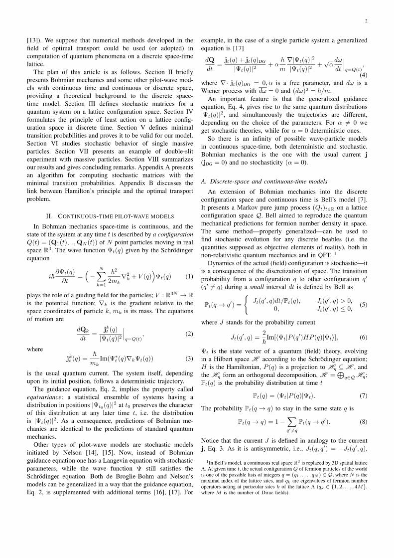
Finally, one can expect convergence to the classical tra-jectories when quantum effects can be neglected (i.e. whenapproximation of wave phenomena by classical mechanics isvalid). Thus, let us study the model in the limit of a shortwavelength. For example, for a wavelength λ = 7 nm we getin a two-slit experiment a set of random trajectories formingtwo independent parallel bunches (Fig. 7). They resembletrajectories of Newtonian (macroscopic) particles which do notpossess wave properties and follow straight lines in an emptyflat space with constant potential V .

8

-0.6 -0.4 -0.2 0 0.2 0.4 0.6

0

0.0025

0.005

0.0075

0.01

x [mm]

y [m

]

Figure 7. Trajectories of single particles in a double-slit experiment for thecase of a short wavelength λ = 7 nm. The width of the slits is a = 0.1mm, the distance between them is d = 0.3 mm. The trajectories form twonarrow bunches as wave properties of particles are negligible, and they behavealmost as classical Newtonian particles. Instead of an interference pattern twoseparated spots appear. The pattern shown at the bottom is built up of particlesimpacts on the screen y = 0.01 m.

VIII. CONCLUSIONS

We have shown how to describe the motion of quantumparticles by a |Ψ|2-distributed Markov process on a lattice indiscrete time. The discreteness is by itself responsible for therandomness of the motion on the basic level, while Hamilton’sprinciple - extended by us to the discrete case - defines thestochastic matrices uniquely. An introduction of any additionalstochastic parameters does not seem to be justified at that levelof description. The consequence of Hamilton’s principle is thatthe stochasticity of the particles’ motion is minimized.

In our approach motion of the system remains randomindependently of the lattice spacings. Introducing Markovianprocess is crucial, if time is discretized. The transformation ofa discrete distribution |Ψt0 |2, e.g. at the slits, into the discretedistribution |Ψt|2, e.g. far from the slits, cannot be made ina non-stochastic manner, as it would require transitions fromevery (initial or intermediate) state into a single subsequentstate. However, such a constraint does not allow the requiredtransformation for discrete distributions to be constructed asin general they change in time.

As an outlook, the model sketched here should be extendedto the Lorentz invariant form and checked in simulations.We can take the Lorentz invariant action in calculations ofS(Pt). However, when we take regular space lattice thenthe stochastic matrices are dependent on that choice, and themodel is not Lorentz invariant. The question is if it can bemade Lorentz invariant, e.g., assuming that discrete spacepoints are placed randomly according to Poisson statistics, asin causal quantum gravity models (see, e.q. [26] and [27]).Yet, the idea of a preferred Lorentz frame is also considered(see, e.g., [28].

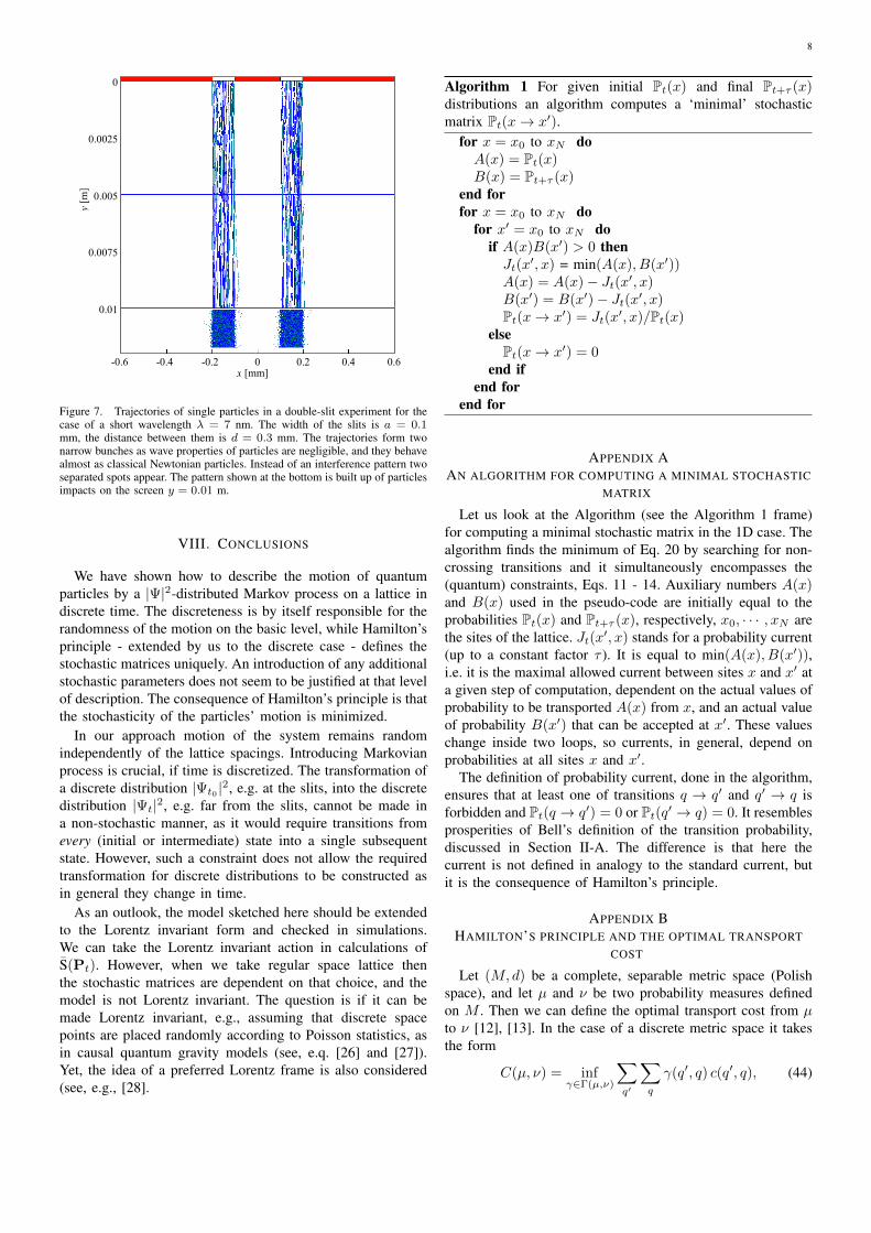
Algorithm 1 For given initial Pt(x) and final Pt+τ (x)distributions an algorithm computes a ‘minimal’ stochasticmatrix Pt(x→ x′).

for x = x0 to xN doA(x) = Pt(x)B(x) = Pt+τ (x)

end forfor x = x0 to xN do

for x′ = x0 to xN doif A(x)B(x′) > 0 thenJt(x

′, x) = min(A(x), B(x′))A(x) = A(x)− Jt(x′, x)B(x′) = B(x′)− Jt(x′, x)Pt(x→ x′) = Jt(x

′, x)/Pt(x)elsePt(x→ x′) = 0

end ifend for

end for

APPENDIX AAN ALGORITHM FOR COMPUTING A MINIMAL STOCHASTIC

MATRIX

Let us look at the Algorithm (see the Algorithm 1 frame)for computing a minimal stochastic matrix in the 1D case. Thealgorithm finds the minimum of Eq. 20 by searching for non-crossing transitions and it simultaneously encompasses the(quantum) constraints, Eqs. 11 - 14. Auxiliary numbers A(x)and B(x) used in the pseudo-code are initially equal to theprobabilities Pt(x) and Pt+τ (x), respectively, x0, · · · , xN arethe sites of the lattice. Jt(x′, x) stands for a probability current(up to a constant factor τ ). It is equal to min(A(x), B(x′)),i.e. it is the maximal allowed current between sites x and x′ ata given step of computation, dependent on the actual values ofprobability to be transported A(x) from x, and an actual valueof probability B(x′) that can be accepted at x′. These valueschange inside two loops, so currents, in general, depend onprobabilities at all sites x and x′.

The definition of probability current, done in the algorithm,ensures that at least one of transitions q → q′ and q′ → q isforbidden and Pt(q → q′) = 0 or Pt(q′ → q) = 0. It resemblesprosperities of Bell’s definition of the transition probability,discussed in Section II-A. The difference is that here thecurrent is not defined in analogy to the standard current, butit is the consequence of Hamilton’s principle.

APPENDIX BHAMILTON’S PRINCIPLE AND THE OPTIMAL TRANSPORT

COST

Let (M,d) be a complete, separable metric space (Polishspace), and let µ and ν be two probability measures definedon M . Then we can define the optimal transport cost from µto ν [12], [13]. In the case of a discrete metric space it takesthe form

C(µ, ν) = infγ∈Γ(µ,ν)

∑q′

∑q

γ(q′, q) c(q′, q), (44)

9

where Γ(µ, ν) denotes the collection of all joint probabilitydistributions γ on M ×M with marginals µ and ν, c(q′, q) isthe so-called cost function on M ×M .

Hamilton’s principle, Eqs. 20 and 21, can be viewed asoptimal transport problem. γ : (q′, q) 7→ Pt(q → q′)Pt(q)make a collection of joint probability distributions on Q×Qwith marginals Pt(q) and Pt+τ (q′), and the cost function isassociated with an action St(q′, q), Eq. 16. So the cost functionbetween an initial point q and a final point q′ is obtainedby minimizing the action among paths that go from q toq′. Finally, an average action S(Pt) is equal to the optimaltransport cost.

When the cost is defined in terms of a distance d, thenthe optimal transport cost can be replaced by the Wassersteindistance

Wp(µ, ν) =

infγ∈Γ(µ,ν)

∑q′

∑q

γ(q′, q) [d(q′, q)]p

1/p

, (45)

where p ≥ 1 is the order of the Wasserstein distance. In sucha case we get in Eq. 35: the total mean square displacementof particles S′(Pt), which is equal to the square of theWasserstein distance of the order p = 2.

There are several numerical methods proposed in the fieldof optimal transport problem (see, e.q. [29], [30], [31]). Wesuppose that they could be adjusted to simulate quantum-mechanical problems more complicated than presented in thispaper, based on Hamilton’s principle in discrete space-time.

ACKNOWLEDGMENT

We would like to thank Marek Gluza, Jas Flaten and PiotrMigdał for many discussions and reading of the manuscript.JK would like to thank his wife Krystyna for her constantsupport and encouragement during the years of research andpreparation of this paper.

REFERENCES

[1] L. de Broglie, La nouvelle dynamique des quanta; in: J. Bordet (Ed.),Electrons et photons. Rapports et discussions du cinquieme Conseil dephysique tenu a Bruxelles du 24 au 29 octobre 1927 sous les auspicesde l’Institut international de physique Solvay (Gauthier-Villars, Paris,1928). English translation is included in: G. Bacciagalluppi and A.Valentini, Quantum Theory at the Crossroads: Reconsidering the 1927Solvay Conference (Cambridge University Press, Cambridge, 2009).

[2] D. Bohm, A Suggested Interpretation of the Quantum Theory in Termsof ”Hidden” Variables, I and II, Phys. Rev. 85, 166 (1952).

[3] D. Durr, S. Goldstein, R. Tumulka, and N. Zanghı, Trajectories andparticle creation and annihilation in quantum field theory, J. Phys. A:Math. Gen. 36, 4143 (2003).

[4] D. Durr, S. Goldstein, R. Tumulka, and N. Zanghı, Bohmian Mechanicsand Quantum Field Theory, Phys. Rev. Lett. 93, 090402 (2004).

[5] D. Durr, S. Goldstein, R. Tumulka, and N. Zanghı, Bell-type quantumfield theories, J. Phys. A: Math. Gen. 38 (4), R1 (2005).

[6] D. Durr, S. Goldstein, and N. Zanghı, Quantum physics without quantumphilosophy ( Springer-Verlag, Berlin, 2013).

[7] J. S. Bell, Beables for quantum field theory, CERN preprint CERN-TH.4035/84; reprinted in [8].

[8] J. S. Bell, Speakable and unspeakable in quantum mechanics(Cambridge University Press, Cambridge, 2004).

[9] A. Vassallo, and M. Esfeld, A proposal for a Bohmian ontology ofquantum gravity, Foundations of Physics 44 (1) 1 (2014).

[10] A Computable Universe: Understanding and Exploring Nature asComputation, H. Zenil (Ed.), (World Scientific, 2013).

[11] J. Barrett, M. Leifer, and R. Tumulka, Bell’s jump process in discretetime, Europhys. Lett. 72 (5), 685 (2005).

[12] L. Ambrosio, N. Gigli, and G. Savare, Gradient flows in metric spacesand in the spaces of probability measures, (Springer Science & BusinessMedia, 2008).

[13] C. Villani, Optimal transport: Old and new, vol. 338 (Springer, VerlagBerlin Heidelberg, 2009).

[14] E. Nelson, Derivation of the Schrodinger equation from Newtonianmechanics, Phys. Rev. 150, 1079 (1966).

[15] E. Nelson, Quantum Fluctuations (Princeton University Press, Dor-drecht, 1985).

[16] E. Deotto and G.C. Ghirardi, Bohmian mechanics revisited, Found. Phys.28, 1 (1998).

[17] G. Bacciagaluppi, Nelsonian Mechanics Revisited, Found. of Phys. Lett.12, 1 (1999).

[18] J. C. Vink, Quantum mechanics in terms of discrete beables, Phys. Rev.A 48 (3), 1808 (1993).

[19] J. S. Bell, On the problem of hidden variables in quantum mechanics,Rev. Mod. Phys. 38 (3), 447 (1966); reprinted in [8].

[20] S. Goldstein, R. Tumulka, and N. Zanghı, Bohmian Trajectories as theFoundation of Quantum Mechanics, in: P. K. Chattaray (Ed.) QuantumTrajectories, (Taylor & Francis, Boca Raton, 2010); arXiv:0912.2666[quant-ph].

[21] D. Durr, S. Goldstein, R. Tumulka, and N. Zanghı, QuantumHamiltonians and Stochastic Jumps, Commun. Math. Phys. 254 129(2005).

[22] L. D. Landau and E. M. Lifshitz, The Classical Theory of Fields(Pergamon Press, Oxford, 1973).

[23] R. P. Feynman and A. R. Hibbs, Quantum Mechanics and Path Integrals(McGraw-Hill, New York, 1965).

[24] P. Ghose, A. S. Majumdar, S. Guha, and J. Sau, Bohmian trajectoriesfor photons, Phys. Lett. A 290 (5), 205 (2001).

[25] C. Philippidis, C. Dewdney, and B. J. Hiley, Quantum interference andthe quantum potential, Il Nuovo Cimento B, Series 11 52 (1), 15 (1979).

[26] J. Henson, The causal set approach to quantum gravity; in: D. Oriti(Ed.), Approaches to Quantum Gravity: Towards a New Understandingof Space, Time and Matter, 393 (Cambridge University Press, New York,2009).

[27] F. Dowker, J. Henson, and R. Sorkin, Quantum Gravity Phenomenology,Lorentz Invariance and Discreteness, Mod. Phys. Lett. A, 19 (24), 1829(2004).

[28] A. Valentini, On Galilean and Lorentz invariance in pilot-wavedynamics, Phys. Lett. A 228 (4), 215 (1997).

[29] C. R. Givens and R. M. Shortt, A class of Wasserstein metrics forprobability distributions, Michigan Math. J., 31 (2), 231 (1984).

[30] L. Ruschendorf, The Wasserstein distance and approximation theorems,Z. Wahrsch. Verw. Gebiete 70 (1), 117 (1985).

[31] G.Ch. Pflug, and A. Pichler, Approximations for Probability Distri-butions and Stochastic Optimization Problems, International Series inOperations Research & Management Science 163, 343 (Springer, NewYork, 2011).