Eur. Phys. J. C manuscript No.(will be inserted by the editor)

Pion Generalized Parton Distributions within a fully covariantconstituent quark model

Cristiano Fanelli a,1, Emanuele Pace b,2, Giovanni Romanelli c,3, Giovanni

Salme d,4, Marco Salmistraro e,5,6,

1Massachusetts Institute of Technology, Laboratory for Nuclear Science, 77 Massachusetts Ave, Cambridge, MA 02139, USA2Phys. Dept. ”Tor Vergata” University and INFN Sezione di Tor Vergata, Via della Ricerca Scientifica 1, 00133 Rome, Italy3STFC, Rutherford-Appleton Lab., Harwell Campus Didcot OX11 0QX, UK4Istituto Nazionale di Fisica Nucleare, Sezione di Roma, P.le A. Moro 2, I-00185 Rome, Italy5Phys. Dept. ”La Sapienza” University, P.le A. Moro 2, I-00185 Rome, Italy6Present addr.: I.I.S. G. De Sanctis, Via Cassia 931, 00189 Rome, Italy

the date of receipt and acceptance should be inserted later

Abstract We extend the investigation of the Gener-

alized Parton Distribution for a charged pion within

a fully covariant constituent quark model, in two re-

spects: (i) calculating the tensor distribution and (ii)

adding the treatment of the evolution, needed for achiev-

ing a meaningful comparison with both the experimen-

tal parton distribution and the lattice evaluation of the

so-called generalized form factors. Distinct features of

our phenomenological covariant quark model are: (i)

a 4D Ansatz for the pion Bethe-Salpeter amplitude,

to be used in the Mandelstam formula for matrix ele-

ments of the relevant current operators, and (ii) only

two parameters, namely a quark mass assumed to hold

mq = 220 MeV and a free parameter fixed through

the value of the pion decay constant. The possibility of

increasing the dynamical content of our covariant con-stituent quark model is briefly discussed in the context

of the Nakanishi integral representation of the Bethe-

Salpeter amplitude.

Keywords Pion Generalized Parton Distributions ·Covariant Constituent Quark Model · Bethe-Salpeter

Amplitude

1 Introduction

The present theory of strong interaction, the Quantum

Chromodynamics (QCD), should in principle allow one

to achieve a complete 3D description of hadrons, in

terms of the Bjorken variable xB and the transverse

ae-mail: cfanelli@mit.edube-mail: emanuele.pace@roma2.infn.itce-mail: giovanni.romanelli@stfc.ac.ukde-mail: salmeg@roma1.infn.itee-mail: marco.salmistraro21@gmail.com

momenta of the constituents. As it is well-known, the

needed non perturbative description still represents a

challenge, that motivates a large amount of valuable ef-

forts, both on the experimental side (gathering new ac-

curate data, that in turn impose stringent constraints

on theoretical investigations) and the theoretical one

(performing more and more refined lattice calculations

and elaborating more and more reliable phenomenolog-

ical models).

Heuristically, while the short-distance behavior of

the hadronic state has been well understood, given the

possibility of applying a perturbative approach, entailed

by the asymptotic freedom, the long-range part of the

hadronic state, that is governed by the confinement, re-

quests non perturbative tools, suitable for a highly non

linear dynamics. Coping with the difficult task to gain

information on the hadronic state, in the whole range of

its extension, has been the main motivation for elabo-

rating phenomenological models, that in general play a

helpful role in shedding light onto the non perturbative

regime.

Among the phenomenological approaches, covari-

ant constituent quark models (CCQMs) represent an

important step forward, since they exploit a quark-

hadron vertex fulfilling the fundamental property of co-

variance with respect to the Poincare group. Moreover,

CCQM’s based on the Light-front (LF) framework, in-

troduced by Dirac in 1949 [1], with variables defined

by: a± = a0±a3 and a⊥ ≡ {ax, ay}, appear to be quite

suitable for describing relativistic, interacting systems,

like hadrons. Indeed, the LF framework has several ap-

pealing features (see, e.g., [2]), quite useful for exploring

nowadays issues in hadronic phenomenology. Beyond

the well-known fact that the dynamics onto the light-

cone is naturally described in terms of LF variables, one

arX

iv:1

603.

0459

8v2

[he

p-ph

] 1

1 A

pr 2

016

2

should mention : (i) the straightforward separation of

the global motion from the intrinsic one (related to the

subgroup property of the LF boosts), (ii) the largest

number of kinematical (i.e. not affected by the interac-

tion) Poincare generators, (iii) the large extent of triv-

iality of the vacuum, within a LF field theory [2] (with

the caveat of the zero-mode contributions). In particu-

lar, for the pion, one can construct the following mean-

ingful Fock expansion onto the null-plane

|π〉 = |qq〉 + |qq qq〉 + |qq g〉.....

where |qq〉 is the valence component. It has to be re-

called that an appealing feature of our approach, based

on a covariant description of the quark-pion vertex (see

[3,4] and references quoted therein), is the possibility

of naturally taking into account contributions beyond

the valence term.

The experimental efforts are very intense for sin-

gling out quantities that are sensitive to the dynamical

features of the hadronic states. In particular, in the last

decade, it has been recognized that a wealth of infor-

mation on the 3D partonic structure of hadrons is con-

tained in the Generalized Parton Distributions (GPDs)

(see, e.g., Ref. [5] for a general presentation), as well

as in the Transverse-momentum Distributions (TMDs)

(see, e.g., Ref. [6] for a detailed discussion). GPDs can

be experimentally investigated through the Deeply Vir-

tual Compton Scattering (DVCS), while TMDs can be

studied through Semi-inclusive Deep Inelastic Scatter-

ing (SIDIS) processes, which notably involve polariza-

tion degrees of freedom.

Our aim, is to provide a phenomenological model,

that has the following main ingredients: (i) a 4D Ansatz

for the pion Bethe-Salpeter amplitude, and (ii) the gen-

eralization of the Mandelstam formula [7] for matrix

elements of the relevant current operators (notice that

the pion Bethe-Salpeter amplitude is needed in this for-

mula). Remarkably, we introduce only two parameters,

namely a constituent quark mass and a free parame-

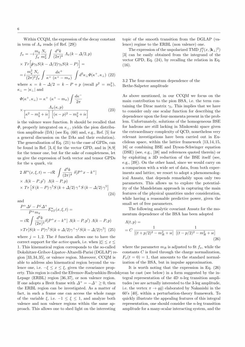
ter fixed through the value of the pion decay constant.

Through our model, we investigate the pion state by

thoroughly comparing the results with both experimen-

tal and lattice data relevant for the 3D description of

the pion. In this paper, we complete the evaluation of

the leading-twist pion GPDs, calculating the so-called

tensor GPD (see Ref. [3] for the vector GPD and Ref. [8,

9] for preliminary calculations of the tensor one). More-

over, in order to accomplish the previously mentioned

comparisons, we consider the evolution of quantities

that can be extracted from the GPDs, like the parton

distribution function (PDF) and the generalized form

factors (GFF). We anticipate that only the leading or-

der (LO) evolution has been implemented by using the

standard code of Ref. [10]. In particular, the compari-

son has been performed between our LO results and the

experimental pion PDF extracted in Ref. [11] (see Ref.

[12] for the NLO extraction) and the available lattice

calculations of GFFs as given in Refs. [13,14,15,16].

The paper is organized as follows. In Sec. 2, the gen-

eral formalism and the definitions are briefly recalled. In

Sec. 3, our Covariant Constituent Quark Model is pre-

sented. In Sec. 4, the LO evolution of the quantities we

want to compare is thoroughly discussed, with a partic-

ular care to the determination of the initial scale of our

model. In Sec. 5, the comparison of our results with

both the experimental PDF and the available lattice

calculations is presented. Finally in Sec. 6, the Conclu-

sion are drawn.

2 Generalities

In this Section, the physical quantities, GPDs and TMDs,

that allow us to achieve a detailed 3D description of a

pion are shortly introduced, since they represent the

target of the investigation within our CCQM (for accu-

rate and extensive reviews on GPDs, see, e.g. [5] and on

TMDs, see, e.g. [6]). For the pion, given its null total

angular momentum, one has two GPDs and two TMDs,

at the leading twist.

2.1 Generalized Parton Distributions

As it is well known, GPDs are LF-boost invariant func-

tions, and allow one to parametrize matrix elements

(between hadronic states) involving quark and gluon

fields. In particular, GPDs are off-diagonal (respect to

the hadron four-momenta, i.e. pf 6= pi,) matrix ele-

ments of quark-quark (or gluon-gluon) correlator pro-

jected onto the Dirac basis (see, e.g., Ref. [17] for a

thorough investigation of the pion case). The appealing

feature of GPDs is given by the ability of summarizing

in a natural way information contained in several ob-

servables investigated in different kinematical regimes,

like electromagnetic (em), form factors (FFs) or PDFs.

The pion has two leading-twist quark GPDs: i) the

vector, or no spin-flip, GPD, HIπ(x, ξ, t), and ii) the ten-

sor, or spin-flip, GPD, EIπ,T (x, ξ, t) (where I = IS, IV

labels isoscalar and isovector GPDs, respectively). In

order to avoid Wilson-line contributions, one can choose

3

the light-cone gauge [5] and get

2

HISπ (x, ξ, t)

HIVπ (x, ξ, t)

=

∫dk−dk⊥

2

×∫dz−dz+dz⊥

2(2π)4ei[(xP

+z−+k−z+)/2−z⊥·k⊥]

× 〈p′|ψq(−1

2z)γ+

1

τ3

ψq(1

2z)|p〉 =

∫dz−

4π

× ei(xP+z−)/2 〈p′|ψq(−

1

2z)γ+

1

τ3

ψq(1

2z)|p〉

∣∣z=0

(1)

and

P+∆j − P j∆+

P+mπ

EISπT (x, ξ, t)

EIVπT (x, ξ, t)

=

∫dz−

4π

× ei(xP+z−)/2 〈p′|ψq(−

1

2z) iσ+j

1

τ3

ψq(1

2z)|p〉

∣∣z=0

(2)

where z ≡ {z+ = z0 + z3, z⊥}, ψq(z) is the quark-field

isodoublet and the standard GPD variables are given

by

x =k+

P+, ξ = − ∆+

2P+, t = ∆2 ,

∆ = p′ − p , P =p′ + p

2(3)

with the initial LF momentum of the active quark equal

to {k+−∆+/2,k⊥−∆⊥/2}. The factor of two multiply-

ing the vector GPD is chosen for normalization purpose,

so that for a charged pion one has

Fπ(t) =

∫ 1

−1

dx HIVπ (x, ξ, t) =

∫ 1

−1

dx Huπ (x, ξ, t) (4)

whereHuπ = HIS

π +HIVπ , andHIS

π is odd in x whileHIVπ

is even (see, e.g. [3]). Finally, it is useful for what follows

to recall the relation with the parton distributions, q(x),

viz

Huπ (x, 0, 0) = θ(x)u(x)− θ(−x)u(−x) . (5)

At the present stage, only a few moments of the

pion GPDs have been evaluated within lattice QCD,

but they represent a valuable test ground for any phe-

nomenological model that aspires to yield meaningful

insights into the pion dynamics. In view of the nu-

merical results discussed below, we briefly recall how

the Mellin moments can be covariantly parametrized

through the GFFs, that are the quantities adopted for

comparing lattice calculations and phenomenological

results.

The relation between the non-spin flip GPD and

the em FF given in Eq. (4) for a charged pion can be

in some sense generalized, if one considers Mellin mo-

ments of both vector and tensor GPDs. Then one ob-

tains the corresponding GFFs. For instance, one can

write the following Mellin moments of both vector and

tensor GPDs for the u-quark (see [5,18] for a review)∫ 1

−1

dxxnHuπ (x, ξ, t) =

[(n+1)/2]∑i=0

(2ξ)2iAun+1,2i(t) , (6)

∫ 1

−1

dxxnEuπ,T (x, ξ, t) =

[(n+1)/2]∑i=0

(2ξ)2iBun+1,2i(t) (7)

where the symbol [...] indicates the integer part of the

argument. In Eqs. (6) and (7), Aun+1,2i(t) is a vector

GFF for a u-quark and Bun+1,2i(t) a tensor GFF, re-

spectively. It is worth noting that one can introduce a

different decomposition in terms of isoscalar and isovec-

tor components instead of a flavor decomposition. In

particular, if n + 1 is even (odd) one has an isoscalar

(isovector) GFF. A striking feature is shown by the rhs

of Eqs. (6) and (7), the so-called polinomiality, i..e. the

dependence upon finite powers of the variable ξ. This

polynomiality property follows from completely general

properties like covariance, parity and time-reversal in-

variance; for this reason it can be a good test for any

model.

By considering the first vector and tensor moments

one gets the following important relations∫ 1

−1

dxHuπ (x, ξ, t) = Au1,0(t) = Fπ(t) (8)

and∫ 1

−1

dxEuπ,T (x, ξ, t) = Bu1,0(t) (9)

where Bu1,0(0) 6= 0 is the tensor charge for n = 0, also

called tensor anomalous magnetic moment (see Ref.

[18]). Notably, Eq. (6) leads to the following relation in-

volving the Mellin moments of the PDF and Aun+1,0(0),

viz

< xn >u=

∫ 1

−1

dxxnHuπ (x, 0, 0) = Aun+1,0(0) (10)

A physical interpretation of GFFs (see, e.g., [19,20,

21]) can be achieved by properly generalizing the stan-

dard interpretation of the non relativistic em FFs to a

relativistic framework. Non relativistically, the em FFs

are the 3D Fourier transforms of intrinsic (Galilean-

invariant) em distributions in the coordinate space (e.g.,

for the pion, one has the charge distribution, while, for

4

the nucleon, one has both charge and magnetic distri-

butions). In the relativistic case, one should consider

Fourier transforms of GPDs, that depend upon vari-

ables invariant under LF boosts. Indeed, only the trans-

verse part of ∆µ can be trivially conjugated to variables

in the coordinate space, while for x and ξ (proportional

to ∆+) this is not possible. Therefore, keeping the de-

scription invariant for proper boosts (i.e. LF boosts),

one can introduce 2D Fourier transforms with respect to

∆⊥. Such a Fourier transform allows one to investigate

the spatial distributions of the quarks in the so-called

impact-parameter space (IPS). In particular, from Eq.

(6) and (7), it straightforwardly follows that, for ξ = 0,

only Aun+1,0(∆2) and Bun+1,0(∆2) survive. Due to the

LF-invariance of ξ, one has an infinite set of frames

(Drell-Yan frames) where ξ = 0. In these frames, where

∆+ = 0 and ∆2 = −∆2⊥, one can introduce the above

mentioned 2D Fourier transforms in a boost-invariant

way (recall that, for a given reaction, the final state or

both final and initial states have to be boosted). One

can write

Aqn(b⊥) =

∫d∆⊥(2π)2

ei∆⊥·b⊥Aqn,0(∆2) ,

Bqn(b⊥) =

∫d∆⊥(2π)2

ei∆⊥·b⊥Bqn,0(∆2) (11)

where b⊥ = |b⊥|, is the impact parameter. In general,

the Fourier transform of GFFs, for ξ = 0, yield quark

densities in the IPS [19,20,21]. In particular, An(b⊥)

represents the probability density of finding an unpo-

larized quark in the pion at a certain distance b⊥ from

the transverse center of momentum. In addition, if one

considers the polarization degrees of freedom, then oneintroduces the probability density of finding a quark

with a given transverse polarization, s⊥ in a certain

Drell-Yan frame. In the IPS, such a probability distri-

bution is

ρqn(b⊥, s⊥) =1

2

[Aqn(b⊥) +

siεijbj

b⊥Γ qn(b⊥)

](12)

where

Γ qn(b⊥) = − 1

2mπ

∂ Bqn(b⊥)

∂ b⊥(13)

It is worth noting that the quark longitudinal (or helic-

ity) distribution density is given only by the first term

in Eq. (12), since the pion is a pseudoscalar meson and

the term γ5/sL in the quark density operator has a van-

ishing expectation value, due to the parity invariance

[16,22].

Equation (12) is quite rich of information and clearly

indicates the pivotal role of GPDs for accessing the

quark distribution in the IPS. Moreover, as a closing

remark, one could exploit the spin-flip GPD EqπT to ex-

tract more elusive information on the quasi-particle na-

ture of the constituent quarks, like their possible anoma-

lous magnetic moments, once the vector current that

governs the quark-photon coupling is suitably improved

(see subsect. 5.4 and Ref. [23] for a discussion within

the lattice framework).

2.2 Transverse momentum distributions

TMDs are diagonal (in the pion four-momentum1) ma-

trix elements of the quark-quark (or gluon-gluon) cor-

relator with the proper Wilson-line contributions (see,

e.g., Ref. [17]) and suitable Dirac structures. Moreover,

TMDs depend upon x and the quark transverse momen-

tum, k⊥, that is not the conjugate of b⊥. It should be

pointed out that in general the Wilson-line effects must

be carefully analyzed, due to the explicit dependence

upon k⊥ (recall that for GPDs such dependence is in-

tegrated out). At the leading-twist, one has two TMDs,

for the pion: the T-even fq1 (x, |k⊥|2), that yields the

probability distribution to find an unpolarized quark

with LF momentum {x,k⊥} in the pion, and the T-

odd hq⊥1 (x, |k⊥|2, η), related to a transversely-polarized

quark and called Boer-Mulders distribution [24].

The two TMDs allow one to parametrize the distri-

bution of a quark with given LF momentum and trans-

verse polarization, i.e. (see, e.g., Ref. [15,17])

ρq(x,k⊥, s⊥, η) =

=1

2

[fq1 (x, |k⊥|2) +

siεijkj⊥mπ

hq⊥1 (x, |k⊥|2, η)]

(14)

where the dependence upon the variable η in h⊥1 is gen-

erated by the Wilson-line effects, whose role is essential

for investigating a non vanishing h⊥1 (see e.g. [24]).

At the lowest order, the unpolarized TMD fq1 , is

given by the proper combination of the isoscalar and

isovector components, that are defined by

2

f IS1 (x, |k⊥|2)

f IV1 (x, |k⊥|2)

=

∫dz−dz⊥2(2π)3

ei[xP+z−/2−k⊥·z⊥]

× 〈p|ψq(−1

2z)γ+

1

τ3

ψq(1

2z)|p〉

∣∣z+=0

, (15)

After integrating over k⊥, one gets the standard unpo-

larized parton distribution q(x), viz

q(x) =

∫dk⊥ f

q1 (x, |k⊥|2) = Hq

1 (x, 0, 0) . (16)

1Notice that ∆µ = (pπf − pπi )µ = 0 leads to ξ = t = 0.

5

The T-odd TMD, h⊥1 (x, |k⊥|2, η) needs a more careful

analysis, since it vanishes at the lowest order in pertur-

bation theory. As a matter of fact, it becomes propor-

tional to the matrix elements

〈p|ψq(−1

2z) i σ+j

1

τ3

ψq(1

2z)|p〉

∣∣z+=0

, (17)

that are equal to zero, due to the time-reversal invari-

ance. In order to get a non vanishing Boer-Mulders dis-

tribution, one has to evaluate at least a first-order cor-

rection, involving Wilson lines (see, e.g., Refs. [25] and

[17]). Moreover, by adopting the light-cone gauge and

the advanced boundary condition for the gauge field,

the effect of the Wilson lines (final state interaction ef-

fects) can be shifted into complex phases affecting the

initial state (see, e.g., Ref. [26]).

3 The Covariant Constituent Quark Model

The main ingredients of our covariant constituent quark

model are two: i) the extension to the GPDs and TMDs

of the Mandelstam formalism [7], originally introduced

for calculating matrix elements of the em current op-

erator when a relativistic interacting system is inves-

tigated, and ii) a model of the 4D quark-hadron ver-

tex, or equivalently the Bethe-Salpeter amplitude, nec-

essary for applying the Mandelstam approach. In par-

ticular, we have assumed a pion Bethe-Salpeter ampli-

tude (BSA) with the following form

Ψ(t, p) = −mfπ

S (t+ p/2) Γ (t, p) S (t− p/2)

(18)

where p = pq+pq is the total momentum, t = (pq−pq)/2the relative momentum of the qq pair (by using the

four-momenta k, ∆ and P previously introduced, one

has t + p/2 = k − ∆/2, and t − p/2 = k − P ). In Eq.

(18), S(pq) = 1/(/pq−mq+ıε) is the fermion propagator

and Γ (t, p) the quark-pion vertex. In the present work,

only the dominant Dirac structure has been assumed,

viz

Γ (t, p) = γ5 Λπ(t, p) (19)

with Λ(t, p) a suitable momentum-dependent scalar func-

tion that contains the dynamical information (see the

following subsections for more details). Indeed, Dirac

structures contributing to Γ (t, p) beyond γ5 should be

taken into account, but they have a minor impact on

the pion BSA, as thoroughly discussed in Ref. [27].

For the sake of completeness, let us recall that the

quark-pion vertex fulfills the homogeneous BS equation

that reads as follows

Γ (t, p) =

=

∫d4t′

(2π)4K(t, t′) S (t′ + p/2) Γ (t′, p) S (t′ − p/2)

(20)

where K(t, t′) is the kernel given by the infinite sum of

irreducible diagrams (see, e.g., [28]).

Finally, it is important to emphasize that our inves-

tigation, based on a covariant description of the quark-

pion vertex, naturally goes beyond a purely valence de-

scription of the pion [3,4].

3.1 The Mandelstam Formula for the electromagnetic

current

The Mandelstam formula allows one to express the ma-

trix elements of the em current of a composite bound

system, within a field theoretical approach [7]. It has

been applied for evaluating the FFs of both pion [29,

30,31] and nucleon [32], obtaining a nice description of

both space- and timelike FFs. Furthermore, it has been

exploited for calculating the vector GPD of the pion [3,

4] and for a preliminary evaluation of the tensor GPD

[8,9].

For instance, in the case of the em spacelike FF of

the pion, the Mandelstam formula, where the quark-

pion vertex given in Eq. (19) is adopted, reads (see,

e.g., Ref. [29,30,31])

jµ = − ıe R

×∫

d4k

(2π)4Λπ(k +∆/2, p′)Λπ(k −∆/2, p)

× Tr[S(k − P )γ5S(k +∆/2)V µ(k, q)S(k −∆/2)γ5]

(21)

where R = 2Ncm2q/f

2π , fπ is the pion decay constant

Nc = 3 the number of colors, mq the CQ mass and

V µ(k, q) the quark-photon vertex, that we have simpli-

fied to γµ in the spacelike region. In presence of a CQ,

one could add to the bare vector current a term pro-

portional to an anomalous magnetic moment, namely a

term like

iκq

2mqσµν∆ν ,

as in Ref. [23] (where it has been adopted an improved

vector current within a lattice framework). It should

be pointed out that the above mentioned anomalous

magnetic moment is not used in the present work.

6

Within CCQM, the expression of the decay constant

in term of Λπ reads (cf Ref. [29])

fπ = −imq

fπ

Ncm2π

∫d4k

(2π)4Λπ(k −∆/2, p)

× Tr[/pγ5S(k −∆/2)γ5S(k − P )

]=

= im2q Nc

(2π)2fπ

∫dκ+

κ+ (κ+ −mπ)

∫d2κ⊥Φ(κ+, κ⊥) (22)

where κ = k − ∆/2 = k − P + p (recall p2 = m2π),

κ⊥ = |κ⊥| and

Φ(κ+, κ⊥) = κ+ (κ+ −mπ)

∫dκ−

2π

× Λπ(κ, p)[κ2 −m2

q + iε] [

(κ− p)2 −m2q + iε

] (23)

is the valence wave function. It should be recalled that

Φ, properly integrated on κ⊥, yields the pion distribu-

tion amplitude (DA) (see Eq. (60) and, e.g., Ref. [5] for

a general discussion on the DAs and their evolution).

The generalization of Eq. (21) to the case of GPDs, can

be found in Ref. [3,4] for the vector GPD, and in [8,9]

for the tensor one, but for the sake of completeness, let

us give the expression of both vector and tensor GPDs

for the u quark, viz

2 Hu(x, ξ, t) = −ıR∫

d4k

(2π)4δ[P+x− k+]

× Λ(k − P, p′) Λ(k − P, p)× Tr

[S (k − P ) γ5S (k +∆/2) γ+S (k −∆/2) γ5

](24)

and

P+∆j − P j∆+

P+mπEuπT (x, ξ, t) =

= iR∫

d4k

(2π)4δ[P+x− k+] Λ(k − P, p′) Λ(k − P, p)

×Tr[S(k − P )γ5S(k +∆/2)γ+γjS(k −∆/2)γ5] (25)

where j = 1, 2. The δ function allows one to have the

correct support for the active quark, i.e. when |ξ| ≤ x ≤1. This kinematical region corresponds to the so-called

Dokshitzer-Gribov-Lipatov-Altarelli-Parisi (DGLAP) re-

gion [33,34,35], or valence region. Moreover, CCQM is

able to address also kinematical region beyond the va-

lence one, i.e. −ξ ≤ x ≤ ξ, given the covariance prop-

erty. This region is called the Efremov-Radyushkin-Brodsky-

Lepage (ERBL) region [36,37], or non valence region.

If one adopts a Breit frame with ∆+ = −∆− ≥ 0, then

the ERBL region can be investigated. As a matter of

fact, in such a frame one can access the whole range

of the variable ξ, i.e. −1 ≤ ξ ≤ 1, and analyze both

valence and non valence regions within the same ap-

proach. This allows one to shed light on the interesting

topic of the smooth transition from the DGLAP (va-

lence) regime to the ERBL (non valence) one.

The expression of the unpolarized TMD fq1 (x, |k⊥|2)

[3] can be easily obtained from the integrand of the

vector GPD, Eq. (24), by recalling the relation in Eq.

(16).

3.2 The four-momentum dependence of the

Bethe-Salpeter amplitude

As above mentioned, in our CCQM we focus on the

main contribution to the pion BSA, i.e. the term con-

taining the Dirac matrix γ5. This implies that we have

to consider only one scalar function for describing the

dependence upon the four-momenta present in the prob-

lem. Unfortunately, solutions of the homogeneous BSE

for hadrons are still lacking in Minkowski space given

the extraordinary complexity of QCD, nonetheless very

relevant investigations have been carried out in Eu-

clidean space, within the lattice framework [13,14,15,

16] or combining BSE and Dyson-Schwinger equation

(DSE) (see, e.g., [38] and references quoted therein) or

by exploiting a 3D reduction of the BSE itself (see,

e.g., [39]). On the other hand, since we would carry on

a comparison with a wide set of data, from both exper-

iments and lattice, we resort to adopt a phenomenolog-

ical Ansatz, that depends remarkably upon only two

parameters. This allows us to explore the potential-

ity of the Mandelstam approach in capturing the main

features of the physical quantities under consideration,

while having a reasonable predictive power, given the

small set of free parameters.

The following analytic covariant Ansatz for the mo-

mentum dependence of the BSA has been adopted

Λ(t, p) =

= C1

[(t+ p/2)2 −m2R + ıε]

1

[(t− p/2)2 −m2R + ıε]

(26)

where the parameter mR is adjusted to fit fπ, while the

constants C is fixed through the charge normalization,

Fπ(t = 0) = 1, that amounts to the standard normal-

ization of the BSA, but in impulse approximation.

It is worth noting that the expression in Eq. (26)

can be cast (see below) in a form suggested by the in-

tegral representation of the 4D n-leg transition ampli-

tudes (we are actually interested to the 3-leg amplitude,

i.e. the vertex π → qq) elaborated by Nakanishi in the

60’s [40], within a perturbation-theory framework. To

quickly illustrate the appealing features of this integral

representation, one should consider the n-leg transition

amplitude for a many-scalar interacting system, and the

7

infinite set of Feynman diagrams contributing to deter-

mine the amplitude itself. In this case, it turns out that

the amplitude is given by the folding of a weight func-

tion (called the Nakanishi weight function) and a de-

nominator (with some exponent) that contains all the

independent scalar products obtained from the n exter-

nal four-momenta. It has to be pointed out that the an-

alytic behavior of the amplitude is fully determined by

such a denominator, and this clearly makes the Nakan-

ishi integral representation a valuable tool for investi-

gating 4D transition amplitudes. For n = 3, one can

apply the integral representation to the vertex func-

tion for a system composed by two constituents, and

explicitly discuss the analytic structure, i.e. the core of

the physical content. Another pivotal motivation that

increases the interest on the Nakanishi framework is

given by the following computational finding: even if

the Nakanishi integral representation has been formally

established by considering the whole infinite set of the

Feynman diagrams contributing to an amplitude, i.e. a

perturbative regime, it has been numerically shown that

also in a non perturbative framework, like the homo-

geneous BSE (relevant for describing bound systems),

the Nakanishi representation plays an essential role for

obtaining actual solutions for the vertex function or,

equivalently, for the BSA. Applying the Nakanishi rep-

resentation as an Ansatz for the solution of the BSE one

can determine the unknown Nakanishi weight function

and achieve a genuine numerical solution of the BSE

in Minkowski space. This approach has been applied

to the ladder BSE for two-scalar and two-fermion sys-

tems (see, e.g.,Refs. [41,42,43,44,45] for the Nakanishi

approach in Minkowski space and, for the sake of com-

parison, Ref. [46,47] for two-fermion systems within the

Euclidean hyperspherical approach), opening a viable

path for phenomenological studies within a non pertur-

bative regime.

Within the Nakanishi approach, the vertex function

(or three-leg amplitude) can be written as follows

Λ(t, p) =

∫ ∞0

dγ

∫ 1

−1

dzg(γ, z;κ2)[

γ + κ2 − t2 − z p · t− iε]2

(27)

where κ2 = m2q−p2/4 and g(γ, z;κ2) is called Nakanishi

weight function. If we take g(γ, z;κ2) = δ(γ−m2R+m2

q),

one obtains Eq. (26). It should be pointed out that while

waiting for numerical solutions of the two-fermion sys-

tem with more refined phenomenological kernels (for

the ladder approximation see Ref. [42]), one could per-

form an intermediate step, still in the realm of Ansatzes,

substituting Eq. (26) with Eq. (27), but adopting a dif-

ferent choice of the Nakanishi weight function, e.g. by

substituting the simple delta-like form with more re-

alistic functions (see e.g. [44] for the Nakanishi weight

functions of a two-scalar system obtained by actually

solving the homogeneous BSE in the ladder approxi-

mation). In order to set the reference line for the next

steps in the elaboration of our CCQM (presented else-

where), we will adopt the very manageable form given

in Eq. (26), in the following comparisons with the ex-

perimental and lattice results (see below, Sec. 5).

4 Evolution of Mellin Moments and GFF’s

In order to compare our results for PDF and GFFs with

experimental data and lattice calculations, it is funda-

mental to suitably evolve the CCQM outcomes, from

the unknown scale µCCQ to the needed ones, namely

µexp and µLAT .

Our strategy for determining an acceptable µCCQis to study the evolution of the non singlet PDF Mellin

within a LO framework, considering flavor numbers up

to Nf = 4. It should be pointed out that the choice to

adopt the LO framework, seems to be well motivated by

the phenomenological nature of the CCQM, and by the

present uncertainties still affecting both experimental

and lattice GFFs.

Let us shortly summarize our procedure for assign-

ing a scale µ to our calculations. The main ingredient

to be considered are the Mellin moments of the non

singlet distribution fNS(x, µ), viz

MNS(n, µ) =

∫ 1

0

dx xn fNS(x, µ) (28)

where fNS is related to the unpolarized GPD, as follows

fNS(x, µCCQ) = 2HI=1(x, 0, 0) (29)

Mellin moments evolve from a scale µ0 to the scale µ

through very simple expressions (see, e.g., [48]), that

for the non singlet, singlet and gluon moments read

dMNS(n, µ)

dlnµ2=αLOs (µ,Nf )

2π

γ(0)qq (n)

2β0MNS(n, µ) (30)

d−→M(n, µ)

dlnµ2=αLOs (µ,Nf )

2π

Γ (0)(n)

2β0

−→M(n, µ) (31)

where

−→M(n, µ) =

(MS(n, µ)

MG(n, µ)

)(32)

In Eqs. (30) and (31), the LO anomalous dimensions

are indicated by γ(0)ab while the 2× 2 matrix Γ (0)(n) is

given by

Γ (0)(n) =

γ(0)qq (n) γ

(0)qG(n)

γ(0)Gq (n) γ

(0)GG(n)

. (33)

8

Let us recall that each anomalous dimension γ(0)ab (n) is

obtained from the corresponding LO splitting function.

In particular, for the unpolarized case, one has (see,

e.g., [48])

γ(0)qq (n) = −8

3

[3 +

2

(n+ 1)(n+ 2)− 4

n+1∑k=1

1

k

](34)

γ(0)qG(n) = −2

[n2 + 3n+ 4

(n+ 1)(n+ 2)(n+ 3)

](35)

γ(0)Gq (n) = −16

3

[n2 + 3n+ 4

n(n+ 1)(n+ 2)

](36)

γ(0)GG(n,Nf ) = −6

[β0(Nf )

3+ 8

n2 + 3n+ 3

n(n+ 1)(n+ 2)(n+ 3)

−4

n+1∑k=1

1

k

]. (37)

where

β0(Nf ) = 11− 2

3Nf (38)

By taking into account the eigenvalues of Γ (0)(n), given

by (see [49] for details)

γ±(n) =1

2

[γ(0)qq (n) + γ

(0)GG(n)

±√

(γ(0)qq (n)− γ(0)

GG(n))2 + 4γ(0)qG(n)γ

(0)Gq (n)

], (39)

one can write the 2 × 2 matrix in terms of projectors

and eigenstates as follows

Γ (0)(n) = γ+(n)P+(n) + γ−(n)P−(n) (40)

with

P±(n) =±1

γ+(n)− γ−(n)[Γ (0)(n)− γ∓(n) I] (41)

They fulfills the usual projector properties, i.e.

P+ + P− = 1

P2± = P±P+P− = P−P+ = 0 (42)

Solutions of Eqs. (30) and (31) are given by

MNS(n, µ) =

[αLOs (µ,Nf )

αLOs (µ0, Nf )

][γ(0)NS(n)/2β0(Nf )]

× MNS(n, µ0) (43)

−→M(n, µ) =

[αLOs (µ,Nf )

αLOs (µ0, Nf )

][Γ (0)(n)/2β0(Nf )]

×−→M(n, µ0) (44)

Notably, Eq. (44) can be put in a more simple form

by using the eigenvalues, γ±, and the corresponding

projectors P±, viz. [49]

−→M(n, µ) =

{[ αLOs (µ,Nf )

αLOs (µ0, Nf )

][γ+(n)/2β0]

P+

+[ αLOs (µ,Nf )

αLOs (µ0, Nf )

][γ−(n)/2β0]

P−} −→M(n, µ0). (45)

Indeed, we are interested to actually evolve only the mo-

ment n = 1 of fNS , since for this moment we can find

several lattice calculations (but using different approxi-

mations; cf Sec. 5). Our procedure requests to backward-

evolve the lattice MLATNS (1, µLAT ), down to a scale µ0

where MLATNS (1, µ0) = MCCQM

NS (1) (notice the absence

of the unknown scale dependence in the CCQM first

moment). This value of the scale is taken as µCCQ.

From Eq. (43), one recognizes the necessity to first

determine αLOs (µLAT , Nf ). This can be accomplished

starting from a reasonable value of αs(µi, 3), like αs(µi =

1 GeV, 3) = 0.68183 given in Ref. [50] (see also Sect. 5

for the quantitative elaboration). To perform this step

we have used the well-known expression

αLOs (µ,Nf ) =αLOs (µi, Nf )

1 +αLOs (µi,Nf )

4π β0(Nf ) ln(µ2/µ2

i

) (46)

It should be pointed out that, as explicitly shown in

Eqs. (38) and (46), αs(µ,Nf ) depends upon the num-

ber of flavors Nf , at a given scale. Indeed, one has to

be particularly careful about the energy scales involved,

when one moves from a relatively low µi = 1 GeV

to µLAT = 2 GeV, large enough to produce a new

quark flavor, so that Nf increases from 3 to 4. In prac-

tice, a two-step procedure has been adopted for moving

from αs(µi, Nf = 3) to αs(µLAT , Nf = 4), by properly

changing β0(Nf ), at the threshold µ = mc, i.e the mass

of the charm.

In what follows, it is also useful to define, at a given

energy scale and number of flavors,

ln(ΛNfQCD) = ln(µ)− 2π

β0(Nf ) αLOs (µ,Nf )(47)

4.1 QCD Evolution of GFFs

Similarly to the more familiar case of PDFs, where

the QCD interaction among partons lead to ultravio-

let divergences which are factored out and absorbed

into a dependence upon the energy scale, also in the

case of GPDs one has to deal with the issue of finding

and solving evolution equations. As a matter of fact,

GPDs do not depend on three variables but on four,

namely H(x, ξ, t, µ) and E(x, ξ, t, µ). However, the evo-

lution kernel does not depend on t, so that the relevant

variables for the evolution are x, ξ, and µ. One should

keep in mind that the evolution of GPDs is produced

9

by the combination of two regimes: (i) the one pertain-

ing to the valence region (|x| > |ξ|) and (ii) the one

pertaining to the non valence region (|x| < |ξ|). One

could roughly say that the evolution of GPDs inter-

polates [5] between the two regions and therefore the

evolution kernel has to take into account the suitable

physical content. In particular, in the valence region a

kernel acts with a structure like the one present in the

DGLAP equations, while in the non valence region a

modified ERBL kernel is involved (see Refs. [51] and

[52] for details on the evolution of vector and tensor

GPDs, respectively).

In our actual comparison, we do not consider the

full GPDs, but rather their Mellin moments, since they

can be in principle addressed by the lattice calculations.

As a matter of fact, GFFs covariantly parametrize the

Mellin moments of GPD (see Eqs. (6) and (7)), and

evolve through a suitable generalization of the Eqs. (43)

and (44) (see Refs. [49,53,54,55,56,57,58]). Let us re-

call, however, that GFFs are the coefficients of poly-

nomials in ξ that yield the Mellin moments of GPDs

and not the Mellin moments themselves: for this reason

in general the equations describing GFFs evolution are

more complicated than Eqs. (43) and (44). Indeed one

can find some notable exceptions where the equations

have a simple multiplicative structure.

For the vector GFFs AIni(t, µ2), one should recall

that the evolution of the isoscalar (singlet) GPD, and

consequently the evolution of the corresponding Mellin

moments, is coupled with the evolution of the gluonic

component. This leads one to separate the evolution of

GFFs with even and odd n, since for symmetry reasons

the even GFFs come from the isoscalar GPDs, while the

odd ones come from the isovector GPDs. By repeating

the main steps given in Ref. [54] (see also [55,56] where

general discussions are presented) for obtaining the evo-

lution equation of both non singlet and singlet vector

GFFs, we can express the results in Ref. [54] also as

follows

A2k+1,2`(t, µ) =Γ (2k + 1)

2

k∑j=k−`

22(j−k)

×k∑

m=j

(4m+ 3)L2m+1(−1)m−j Γ (j +m+ 3/2)

Γ (2j + 1)

×A2j+1,2(j−k+`)(t, µ0)

Γ (m− j + 1)Γ (k −m+ 1)Γ (k +m+ 5/2)(48)

with 0 ≤ ` ≤ k and

L2m+1 =

(αs(µ,Nf )

αs(µ0, Nf )

)[γ(0)qq (2m)/2β0(Nf )]

. (49)

For the singlet vector GFFs we get

A2k+2,2`(t, µ) = Γ (2k + 2)

k∑j=k−`

22(j−k)−1

×k∑

m=j

(4m+ 5)L2m+2(−1)m−j Γ (j +m+ 5/2)

Γ (2j + 2)

×A2(j+1),2(j−k+`)(t, µ0)

Γ (m− j + 1)Γ (k −m+ 1)Γ (k +m+ 7/2)(50)

with 0 ≤ ` ≤ k + 1, A00 = 0 and

L2m+2 =

(αs(µ,Nf )

αs(µ0, Nf )

)[Γ(0)V (2m+1)/2β0(Nf )]

(51)

where Γ(0)V is the same 2 × 2 matrix defined in (33)

that depends upon Nf through γ(0)GG. In Eqs. (48) and

(50), Γ (k) is the usual Euler function. Notice that the

dependence upon t in the GFF is not involved in the

evolution. Some example of explicit evolution equations

are

An0(t, µ) = Ln An0(t, µ0)

A22(t, µ) = L2 A22(t, µ0) (52)

where A22(t, µ) is a 2D vector, with quark and gluon

components, and L2 a 2 × 2 matrix. For An0(t, µ) the

evolution equations become exactly equal to Eqs. (43)

and (44) for the odd and even n’s respectively. More-

over, since γ(0)qq (n = 0) = 0 then L1 = 1. This is ex-

pected since A10(t = 0) is the charge (A10(t) is the em

form factor), namely a measurable quantity and there-

fore it cannot evolve.

For the tensor GFF BIni(t, µ), analogous arguments

can be carried out, but with a great simplification. In

fact, at LO the gluon-quark and quark-gluon transi-

tion amplitudes that lead to the corresponding splitting

functions are vanishing for the helicity conservation (re-

call that ET (x, ξ, t) is related to an expectation value

with a transversely polarized quark and describes helic-

ity flip transitions), therefore the anomalous dimension

matrix Γ(0)T (n) is diagonal. Consequently, at LO it is not

necessary to separate the case of even and odd n, since

there is no mixing between quark and gluon evolutions,

and one can eventually write the evolution equation in

a form analogous to Eq. (48). In particular, the quark

component of the transverse GFFs, Bqn0(t, µ), evolves

multiplicatively (see, e.g., [49,57,58,59]), viz

Bqn0(t, µ) = LqTn Bqn0(t, µ0). (53)

where

LqTn =

(αs(µ,Nf )

αs(µ0, Nf )

)[γ(0)qqT (n−1)/2β0(Nf )]

(54)

10

with a transverse anomalous dimension (notice a factor

of 2 difference with [49], due to the different normaliza-

tion) given by

γ(0)qqT (`) = − 8

3

[3− 4

`+1∑k=1

1

k

]. (55)

For the sake of completeness, the gluon transverse LO

anomalous dimension reads

γ(0)ggT (`) = − 6

[β0(Nf )

3− 4

`+1∑k=1

1

k

]. (56)

5 Numerical Results

The reliability of the quark-pion vertex (26), introduced

for obtaining the Bethe-Salpeter amplitude (18), has

been first checked by comparing our results for a charged

pion with the most accurate experimental data not af-

fected by the evolution, i.e. the spacelike em form fac-

tor. Theoretically, the em form factor, Fπ(t), is given

by the GFF A10(t). In Fig. (1) the results obtained by

different models for the em FF are shown as a function

of (−t), together with the experimental data. To avoid

the use of a log plot, that prevents a detailed analysis,

the FF has been divided by the monopole function

Fmon(t) =1

1 + |t|/m2ρ

(57)

where mρ = 0.770 GeV. Interestingly, in order to test

the dependence upon the CQ mass, the results of our

CCQM evaluated for quark masses mq = 0.200, 0.210,

0.220 GeV, have been also shown, together with (i) the

results from a LF CQM where mq = 0.265 GeV and a

dressed quark-photon vertex were adopted [30,31]; (ii)a fit to the lattice data obtained in [23]. It has to be

pointed out that the fit to the lattice data was pre-

sented in [23] itself, and it has the following monopole

expression

F latπ (t) =1

1− t/M2(mphysπ )

(58)

with M(mphysπ ) = 0.727 GeV. The lattice results were

actually obtained for a pion mass mπ = 0.600 GeV, and

then extrapolated to the physical pion mass mphysπ =

0.140 GeV, up to t = −4 GeV2 (see [23]). In Fig.

(1), for the sake of presentation, the monopole fit (58)

has been arbitrarily extended up to t = −10 GeV2.

Once the CQ mass is assigned, our CCQM model de-

pends upon only one free parameter, the regulator mass

mR in Eq. (26). The value of mR is fixed by calcu-

lating the pion decay constant fπ (cf Eq. (22)), while

the constant C is determined through Fπ(0), as al-

ready mentioned in subsec. 3.2. The PDG experimen-

tal value fexpπ = 0.0922 GeV [60] has been adopted.

In particular, for mq = 0.200, 210, 220 GeV, we got

mR = 1.453, 1.320, 1.192 GeV, respectively.

The following comments are in order: (i) a nice agree-

ment between the CCQM results and the experimental

FF at low momentum transfer leads to reproduce the

experimental value of the charge radius, < r2exp >=

0.67± 0.02 fm; (ii) beyond −t = 0.5 GeV2, CCQM re-

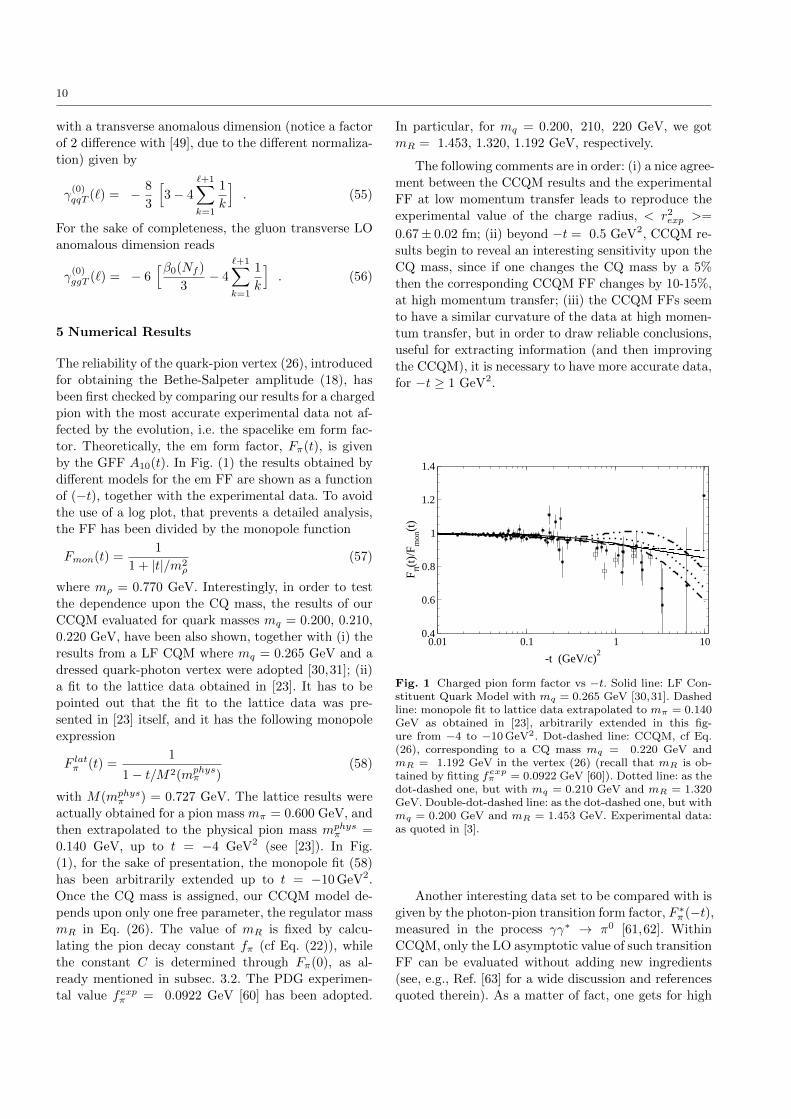
sults begin to reveal an interesting sensitivity upon the

CQ mass, since if one changes the CQ mass by a 5%

then the corresponding CCQM FF changes by 10-15%,

at high momentum transfer; (iii) the CCQM FFs seem

to have a similar curvature of the data at high momen-

tum transfer, but in order to draw reliable conclusions,

useful for extracting information (and then improving

the CCQM), it is necessary to have more accurate data,

for −t ≥ 1 GeV2.

0.01 0.1 1 10-t (GeV/c)2

0.4

0.6

0.8

1

1.2

1.4

F π(t)/F

mon

(t)

Fig. 1 Charged pion form factor vs −t. Solid line: LF Con-stituent Quark Model with mq = 0.265 GeV [30,31]. Dashedline: monopole fit to lattice data extrapolated to mπ = 0.140GeV as obtained in [23], arbitrarily extended in this fig-ure from −4 to −10 GeV2. Dot-dashed line: CCQM, cf Eq.(26), corresponding to a CQ mass mq = 0.220 GeV andmR = 1.192 GeV in the vertex (26) (recall that mR is ob-tained by fitting fexpπ = 0.0922 GeV [60]). Dotted line: as thedot-dashed one, but with mq = 0.210 GeV and mR = 1.320GeV. Double-dot-dashed line: as the dot-dashed one, but withmq = 0.200 GeV and mR = 1.453 GeV. Experimental data:as quoted in [3].

Another interesting data set to be compared with is

given by the photon-pion transition form factor, F ∗π (−t),measured in the process γγ∗ → π0 [61,62]. Within

CCQM, only the LO asymptotic value of such transition

FF can be evaluated without adding new ingredients

(see, e.g., Ref. [63] for a wide discussion and references

quoted therein). As a matter of fact, one gets for high

11

(−t), at LO in pQCD,

(−t) F ∗π (−t)→ 2fπ3

∫ 1

0

dξφπ(ξ, |t|)

ξ(59)

where φπ(ξ, |t|) is the pion DA evaluated at the scale

|t|. The CCQM result (with an undetermined scale for

the moment, see the next subsection) is given by

φπ(ξ, µ2CCQM ) = i

m2qNc

f2πmπ(2π)2

× 1

ξ(1− ξ)

∫ ∞0

d2κ⊥ Φ(ξmπ, κ⊥) (60)

where Φ(ξmπ, κ⊥) is defined in Eq. (23). The normaliza-

tion of φπ follows from Eq. (22). It should be anticipated

that CCQM results, both non evolved and evolved, as

shown in the next Fig. 3, resemble the asymptotic pion

DA obtained within the pQCD framework, i.e. φasyπ (ξ) =

6ξ(1 − ξ), that in turn yields (−t) F ∗π (−t) → 2fπ, see

Refs. [64,65].

In what follows, the values mq = 0.220 geV and

mR = 1.192 GeV will be adopted.

5.1 Looking for the CCQM energy scale

As it is well-known, the em FF is not affected by the

issue of the evolution, while the other quantities we are

interested in, namely the PDF and the GFFs (as well

as the DA, see Eq. (60)), have to be properly evolved.

A necessary step for going forward is to assign a

resolution scale to CCQM. In order to perform this

step, we have taken lattice estimates of the first Mellin

moment of fNS(x, µ), whose evolution is determined

only by the quark contribution, as normalization of our

CCQM (roughly speaking). The starting point is the

calculation of both the unpolarized GPD, fNS(x) =

2HI=1(x, 0, 0), and the corresponding Mellin moments,

within our CCQM. In particular, these quantities are

shown in Table 1 up to n = 3. To emphasize that there

is no direct way to gather information about the energy

scale µ0, a question mark is put in the Table. In the

Table 1 Mellin moments of fNS(x) up to n = 3, evaluatedwithin the CCQM with the quark pion vertex given in Eq.(26), mq = 0.220 GeV, and mR = 1.192 GeV. The energyscale, µ0 has to be determined (see text).

µ0 < x > < x2 > < x3 >

? 0.471 0.276 0.183

literature there are various lattice results for the first

moment at the energy scale of µ = 2 GeV, and we have

exploited the ones shown in Tab. 2. It is worth notic-

ing that the lattice results are not too far from a phe-

nomenological estimate, < x >phe (µ = 2 GeV), that

one can deduce by applying a LO backward-evolution to

the value given in Ref. [12], < x >phe (µ = 5.2 GeV) =

0.217(11), obtained after a NLO re-analysis of the Drell-

Yan data of Ref. [11]. In particular, the phenomenolog-

ical value at µ = 2 GeV is

< x >phe (µ = 2 GeV) = 0.260(13)

For the sake of completeness, it is interesting to quote

Table 2 Recent lattice results for the first Mellin moment ofthe non singlet fNS(x), at the energy scale µLAT = 2 GeV.The first and the second lines are the results obtained fromunquenched lattice QCD calculations [14,66], while the thirdresult has been obtained in quenched lattice QCD [67].

Ref. µLAT [GeV ] < x >LAT

Lat. 07 [14] 2.0 0.271(10)South [66] 2.0 0.249(12)χLF [67] 2.0 0.243(21)

two other lattice calculations: (i) the quenched one of

Ref. [68] that amounts to a value < x >LAT (µ =

2 GeV) = 0.246(15), i.e. falling between the results of

Refs. [66,67] and (ii) a very recent lattice estimate, re-

markably at the physical pion mass, giving < x >LAT(µ = 2 GeV) = 0.214(19) [69].

After establishing the set of lattice data, we need the

value of αLOs at µ = 2 GeV where Nf = 4. This value

has been obtained starting from αLOs (µ = 1 GeV) =

0.68183 obtained in Ref. [50]. Notice that at the scale

µ = 1 GeV only three flavors are active. Then, by us-

ing mc = 1.4 GeV [50] and Eq. (46), with the proper

β0(Nf ), one determines αLOs (µ = 2 GeV, 4) = 0.413

(see also Refs. [60,70,71], where the crossing of the fla-

vor threshold has been discussed). Finally, paying at-

tention to the flavor threshold, the lattice evaluations of

the first moment MLATNS (1, µLAT ) have to be backward-

evolved up to a scale µ0, where they match our CCQM

value, i.e. we look for µ0 such that MLATNS (1, µ0) =

0.471 = MCCQMNS (1, ?). In detail, we calculate first (cf.

Eq. (43)) the lattice result at the charm mass scale, viz

MNS(1,mc) =

[αLOs (mc, 4)

αLOs (µLAT , 4)

]γ(0)qq (1)/(2β0(4))

× MNS(1, µLAT ) (61)

where γ(0)qq (1) = 64/9, β0(4) = 25/3, αLOs (mc, 4) =

0.513 (corresponding to ΛQCD(Nf = 4) = 0.322 GeV)

and MNS(1, µLAT ) are the values shown in Tab. 2.

12

Table 3 Energy scale of CCQM, µ0, as determined from (i) the first Mellin moments calculated within a lattice frameworkin Refs. [14,66,67] and (ii) the CCQM result, < x >= 0.471, calculated with mq = 0.220 GeV and mR = 1.192 GeV. For all

the three calculations shown in the Table, one gets ΛNf=3

QCD (µ0) = 0.359 GeV from Eqs. (47) and (63).

Ref. < x >LAT µ0 [GeV] αLOs (µ0, 3)

Lat. 07 [14] 0.271 0.549 1.64South [66] 0.249 0.506 2.04χLF [67] 0.243 0.496 2.17

Table 4 Comparison for the second and third Mellin mo-ments of the non singlet fNS(x), at the energy scale µLAT =2 GeV, between the unquenched lattice results of Ref. [14]and the evolved CCQM, where the theoretical uncertaintyis generated by the three values for the CCQM initial scaleshown in Tab. 3

< x2 > < x3 >

Lat. 07 [14] 0.128(18) 0.074(27)CCQM 0.105(11) 0.055(7)

Once MNS(1,mc) is obtained, αLOs (µ0) can be eval-

uated through (cf. Eq. (43))

αLOs (µ0, 3) = αLOs (mc, 3)

×[MNS(1, µ0)

MNS(1,mc)

]−γ(0)qq (1)/(2β0(3))

, (62)

where MNS(1, µ0) corresponds to our CCQM calcula-

tion and β0(3) = 9. After determining αLOs (µ0, 3), µ0 is

easily found through

ln

(µ0

µ = 1 GeV

)=

2π

β0(3)

×[ 1

αLOs (µ0, 3)− 1

αLOs (µ = 1 GeV, 3)

](63)

The results for µCCQ obtained from the above pro-

cedure, applied to the three lattice data, are shown in

Tab. 3 for mq = 0.220 GeV and mR = 1.192 GeV. In

particular, the values in the third column of Tab. 3 are

used in the next sections as starting values for the evo-

lution of both the non singlet PDF and the GFFs. The

difference between the three values of µ0 in the Tab. 3

is assumed as a theoretical uncertainty of our results.

To complete this subsection, in Tab. 4, the comparison

with the lattice calculation of Ref. [14] for the second

and the third Mellin moments is presented.

0 0.1 0.2 0.3 0.4 0.5 0.6 0.7 0.8 0.9 1x

0

0.2

0.4

0.6

0.8

xfN

S(x)

Fig. 2 Evolution of the non singlet parton distribution.Dashed line: non evolved PDF obtained from CCQMHI=1(x, 0, 0) with a CQ mass mq = 0.220 GeV and mR =1.192 GeV in the vertex (26). Solid line: PDF LO-evolved atµ = 4 GeV from µ0 = 0.549 GeV. Dot-dashed line: PDF LO-evolved at µ = 4 GeV from µ0 = 0.496 GeV. For details onthe values of µ0 see text and Tab. 3. Full dots: experimentaldata at the energy scale µ = 4 GeV, as given in Ref. [11]

5.2 The evolution of the non singlet PDF and the

comparison with the experimental data

The non singlet PDF, as already explained, is the sim-

plest to be evolved since one does not need information

on the gluon distribution. The evolution has been per-

formed using the FORTRAN code described in [10] that

adopts a brute force method to solve the LO DGLAP

equation for the distribution xfNS(x), and it requests

as input the values of (i) µ, the final scale, and (ii) the

initial ΛNfQCD and µ0, as given in Table 3. It should be

pointed out an important detail in our calculations. For

all the values of µ0, the evolution has been performed

in two steps: first xfCCQMNS (x) has been evolved from

µ0 up to mc = 1.4 GeV and then from mc up to µ = 4

GeV, the energy scale of the experimental data [11].

This is necessary for taking into account the variation

13

of Nf , ΛQCD(recall that ΛNf=4QCD (µ = 2 GeV ) is 0.322

GeV) and consequently αLOs (µ).

In Fig. 2, the dashed line is the non evolved CCQM

calculation with mq = 0.220 GeV and mR = 1.192

GeV, while the solid and the dot-dashed lines corre-

spond to our evolved CCQM starting from the initial

scales µ0 = 0.549 GeV and µ0 = 0.496 GeV, respec-

tively. The differences between the evolved calculations

can be interpreted as the theoretical uncertainty of our

calculations. However it is very interesting that our LO-

evolved calculations nicely agree with the experimen-

tal data of Ref. [11] for x > 0.5 (see also the same

agreement achieved within the chiral quark model of

Ref. [53]). On the other hand, it has to be pointed out

that refined calculations, like (i) the ones of Refs. [72,

73] based on the Euclidean Dyson-Schwinger equation

for the self-energy and (ii) the NLO calculation of Ref.

[74] based on a soft-gluon resummation, underestimate

the PDF tail of the experimental data from Ref. [11],

while agree with the analysis of the same experimen-

tal data carried out in Ref. [12], within a NLO frame-

work. The reanalysis of the experimental data leads to

a tail for large x that has a rather different derivative

with respect to the original data from Ref. [11]. For the

0 0.1 0.2 0.3 0.4 0.5 0.6 0.7 0.8 0.9 1 ξ

0

0.5

1

1.5

φπ (ξ

,µ)

Fig. 3 Evolution of the pion distribution amplitude. Solidline: non evolved DA obtained from our CCQM with mq =0.220 GeV and mR = 1.192 GeV in the vertex (26) (see Eqs.(23) and (60)). Dashed line: DA LO-evolved at µ = 1 GeV.Dot-dashed line: PDF LO-evolved at µ = 6 GeV. Dotted line:pQCD asymptotic DA, given by φπ(ξ) = 6ξ(1− ξ).

sake of completeness, in Fig. 3, the CCQM pion DA is

presented together with the results at the energy scale

µ = 1 GeV and µ = 6 GeV. It is worth noticing that

our CCQM evolves toward the pQCD asymptotic pion

DA φπ(ξ) = 6 ξ (1− ξ) (see, e.g., [64,65]) as the energy

scale increases. Analogous results are obtained within

the chiral quark model of Ref. [75].

5.3 The tensor GPD

We have extended to the tensor GPD our CCQM model

already applied to the vector GPD in Refs. [3,4], and

in Fig. 4, our final results are shown for some values

of the variable ξ and t, but for 0 ≤ x ≤ 1 (preliminary

results were presented in Refs. [8,9]). The GPD for neg-

ative values of x can be obtained by exploiting the fact

that EISπT (x, ξ, t) is antisymmetric if x → − x, while

EIVπT (x, ξ, t) is symmetric (see, e.g. Ref. [5] for details).

It has to be pointed out that for ξ → 0 the valence com-

ponent is dominant (DGLAP regime) while for ξ → 1

the non valence term is acting (ERBL regime). In view

of that, it is expected a peak around x ∼ 1 for ξ → 1,

as discussed in Refs. [3,4] for the vector GPD.

It is worth mentioning that both isoscalar and isovec-

tor tensor GPD calculated within the chiral quark model

of Ref. [58] qualitatively show the same pattern (see

also Ref. [8] and reference therein quoted for a compar-

ison with results obtained within the LF Hamiltonian

Dynamics framework).

5.4 The evolution of the GFFs and the comparison

with lattice data

The first vector GFF Aq10, i.e. the em FF, is experimen-

tally known, while the other GFFs can be investigated

only from the theoretical side. In particular, Aq20(t, µ),Aq22(t, µ), Bq10(t, µ) and Bq20(t, µ) have been calculated

within the lattice framework at the scale µ = 2 GeV

[13,15,16]. In this subsection, the comparison between

our CCQM predictions and the above mentioned lat-

tice evaluations is presented. It is important to notice

that other model calculations of both vector and tensor

GFFs are available in the literature (see, e.g., [57,58,

59,75,76,77]).

To proceed, we have calculated both vector and ten-

sor GPDs, and then we have extracted the relevant

GFFs, by exploiting the polynomiality shown in Eqs.

(6) and (7) (see also [3]). The main issue to be ad-

dressed in order to perform the mentioned comparison

with the lattice data is the evolution of our calculations

up to µLAT = 2 GeV. In the simpler case, represented

by the tensor GFFs, the LO evolution of the quark con-

tribution is uncoupled from the gluon one. In particu-

lar, the two-step procedure µCCQ → mc → µLAT has

been adopted for evolving the two transverse GFFs,

Bq10(t, µ0) and Bq20(t, µ0), through Eq. (53). The needed

14

0 0.5 1x

0

0.05

0.1

0.15

0.2

ET

IS(

x , ξ

, t )

0 0.5 1x

0

0.05

0.1

0.15

0.2

ET

IV(

x , ξ

, t )

Fig. 4 Isoscalar and isovector tensor GPDs for a charged pion, within CCQM, for positive x. The behavior for negative valuesof x can be deduced from the antisymmetry of EISπT (x, ξ, t) and the symmetry of EIVπT (x, ξ, t), respectively. Thick solid line:ξ = 0 and t = 0. Thick dotted line: ξ = 0 and t = −0.4GeV 2. Thick dashed line: ξ = 0 and t = −1GeV 2. Thin dotted line:ξ = 0.96 and t = −0.4GeV 2. Thin dashed line: ξ = 0.96 and t = −1GeV 2.

transverse anomalous dimensions are given by (cf. Eq.

(55))

γ(0)qqT (0) =

8

3, γ

(0)qqT (1) = 8 . (64)

Then, for µCCQ ≤ µ < mc one has Nf = 3 and gets

Bq10(t,mc) = Bq10(t, µCCQ)

[αLOs (mc, 3)

αLOs (µCCQ, 3)

]4/27

(65)

Bq20(t,mc) = Bq20(t, µCCQ)

[αLOs (mc, 3)

αLOs (µCCQ, 3)

]4/9

(66)

For mc ≤ µ ≤ µLAT , the flavor number is Nf = 4 and

one has

Bq10(t, µLAT ) = Bq10(t,mc)

[αLOs (µLAT , 4)

αLOs (mc, 4)

]4/25

(67)

Bq20(tµLAT ) = Bq20t, (mc)

[αLOs (µLAT , 4)

αLOs (mc, 4)

]12/25

. (68)

In the case of A20(t, µ) and A22(t, µ) the evolution

equation is more complicated, since both GFFs evolve

through the following expression−→A 2i(t, µ) = L2

−→A 2i(t, µ0) (69)

where, for both scales, one has

−→A 2i =

Aq2i

AG2i

(70)

From the definition (51), the exponent in L2 is a 2× 2

matrix, (see also Eqs. (33), (34), (35), (36) and (37))

that for Nf = 3 reads

Γ(0)V (1) =

γ(0)qq (1) γ

(0)qG(1)

γ(0)Gq (1) γ

(0)GG(1)

=

649 − 2

3

− 649 4

(71)

with eigenvalues (see Eq. (39))

γ± =50± 2

√145

9. (72)

At the valence scale, the gluon contribution is van-

ishing, and therefore one has < x >q= 1/2. Indeed,

the CCQM result amounts to < x > (µCCQ) = 0.47,

namely the momentum sum rule is not completely sat-

urated by the valence component at the CCQM scale

µCCQ. This difference originates from the fact that we

have a covariant description of the pion vertex, and

therefore we have not only a contribution from the va-

lence LF wave function (i.e. the amplitude of the Fock

component with the lowest number of constituents), but

also from components of the Fock expansion of the pion

state beyond the constituent one, like |qq; qq〉. Without

the gluon term at the initial scale (the assumed valence

one), Aq2i(t,mc) is given by (cf. Eqs. (40) and (41))

Aq2i(t,mc) =1

2√

145Aq2i(t, µCCQ) R25/81

3

×[(7 +

√145) R

√145/81

3 − (7−√

145) R−√

145/813

],

(73)

where

R3 =αLOS (mc, 3)

αLOs (µCCQ, 3), (74)

and AG2i(t,mc) reads

AG2i(t,mc) = − 16√145

Aq2i(t, µCCQ) R25/813

×[R√

145/813 −R−

√145/81

3

](75)

For Nf = 4, Eq. (73) changes, since both β0 and γ(0)GG(1)

depend on the flavor number. Therefore Γ(0)V (1) be-

15

comes

Γ(0)V (1) =

649 − 2

3

− 649

163

(76)

with eigenvalues

γ± =56± 8

√7

9(77)

Then, the evolution in the second step from mc →µLAT = 2 GeV reads

Aq2i(t, µ) =R28/75

4

2√

7

×{Aq2i(t,mc)

[(1 +

√7)R4

√7/75

4 − (1−√

7)R−4√

7/754

]−3

4AG2i(t,mc)

[R4√

7/754 −R−4

√7/75

4

]}(78)

where

R4 =αLOS (µ, 4)

αLOs (mc, 4). (79)

It should be pointed out that the GFFs Aq2i evolve mul-

tiplicatively (recall that the evolution is not influenced

by the value of t), given the absence of the gluon con-

tribution at the valence scale, viz

Aq2i(t, µ) = Aq2i(t, µCCQ) F (µCCQ,mc, µ) . (80)

From Eq. (80), one realizes that the ratio

Aq2i(t, µ)/Aq2i(t = 0, µ)

(Aq2i(t = 0, µ) is also called charge) can be compared

with the same ratio obtained at a different scale, e.g.

at µCCQ. It is understood that the same holds for the

tensor GFF. In Figs. 5 and 6, the tensor GFFs Bq10(t)

and Bq20(t), normalized to their own charges, are shown

for both the CCQM model, with mq = 0.220 GeV

and mR = 1.192 GeV, and the lattice framework [13,

16]. In particular the lattice data are represented by a

shaded area, generated by the envelope of curves that

fit the lattice data with their uncertainties. In Refs. [13,

16], the lattice data have been first extrapolated to the

physical pion mass through a simple quadratic (in mπ)

expression, and then fitted by the following pole form

GFFLATj (t)

GFFLATj (0)=

1[1 + t/(pj M2

j )]pj (81)

where pj and Mj are pairs of adjusted parameters,

shown in Tab. 5, for the sake of completeness.

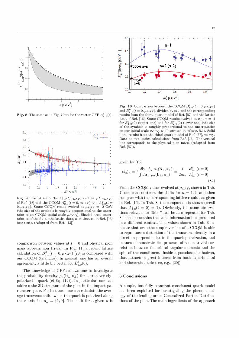
In Figs. 7 and 8, the CCQM A2,0(t) and A2,2(t)

(with CCQM parameters different from the ones adopted

in Ref. [3]) are presented together with the correspond-

ing lattice results.

If one is interested in a comparison that involves

the full GFFs, then it is necessary to specify the scale

Table 5 Adjusted parameters for describing the extrapo-lated lattice data through Eq. (81), as given in Refs. [13,16]

GFF pj Mj

Aq20(t) 1 1.329± 0.058Aq22(t) 1 0.89± 0.25Bq10(t) 1.6 0.756± 0.095Bq20(t) 1.6 1.130± 0.265

0 1 2 3 4-t [GeV

2]

0

0.2

0.4

0.6

0.8

1

BI=

1 (1,0

)(t)/

BI=

1 (1,0

)(0)

Fig. 5 The tensor GFF Bq1,0(t), an isovector one, normalizedto its own charge. Dashed line: CCQM result, correspondingto mq = 0.220 GeV and mR = 1.192 GeV in the vertex (26).The shaded area indicates the lattice data [16] extrapolatedto the pion physical mass mπ = 0.140 GeV (see text).

Table 6 Values at t = 0 of the CCQM GFFs, Aq2,0(0),

Aq2,2(0), Bq1,0(0) and Bq2,0(0).

Aq2,0(0) Aq2,2(0) Bq1,0(0) Bq2,0(0)

0.4710 -0.03308 0.1612 0.05827

and, accordingly, to evolve our CCQM results. In par-

ticular, since we have a multiplicative evolution, it is

sufficient (i) to evolve only the value at t = 0, namely

the ones collected in Tab. 6, through Eqs. (65), (66),

(67), (68), (73) and (78) and then (ii) to use Eq. (80).

As in the case of the evolution of the PDF, we con-

sidered the three possible values of µ0 listed in Tab. 3.

The results are shown in Tab. 7, together with lattice

data [13,16,78] and model calculations, obtained from

a chiral quark model [57,76] and an instanton vacuum

model [59]. It should be pointed out that within the

chiral perturbation theory (see Ref. [79]) one should

have the following relation between the so-called grav-

16

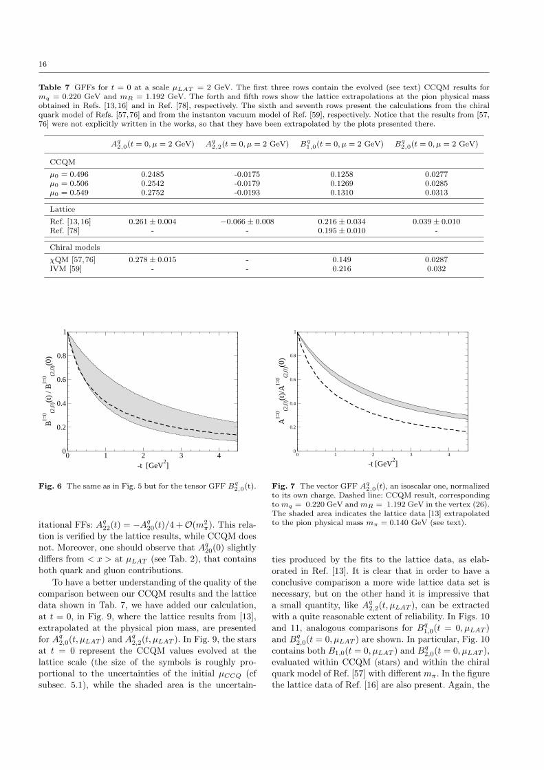
Table 7 GFFs for t = 0 at a scale µLAT = 2 GeV. The first three rows contain the evolved (see text) CCQM results formq = 0.220 GeV and mR = 1.192 GeV. The forth and fifth rows show the lattice extrapolations at the pion physical massobtained in Refs. [13,16] and in Ref. [78], respectively. The sixth and seventh rows present the calculations from the chiralquark model of Refs. [57,76] and from the instanton vacuum model of Ref. [59], respectively. Notice that the results from [57,76] were not explicitly written in the works, so that they have been extrapolated by the plots presented there.

Aq2,0(t = 0, µ = 2 GeV) Aq2,2(t = 0, µ = 2 GeV) Bq1,0(t = 0, µ = 2 GeV) Bq2,0(t = 0, µ = 2 GeV)

CCQM

µ0 = 0.496 0.2485 -0.0175 0.1258 0.0277µ0 = 0.506 0.2542 -0.0179 0.1269 0.0285µ0 = 0.549 0.2752 -0.0193 0.1310 0.0313

Lattice

Ref. [13,16] 0.261± 0.004 −0.066± 0.008 0.216± 0.034 0.039± 0.010Ref. [78] - - 0.195± 0.010 -

Chiral models

χQM [57,76] 0.278± 0.015 - 0.149 0.0287IVM [59] - - 0.216 0.032

0 1 2 3 4-t [GeV

2]

0

0.2

0.4

0.6

0.8

1

BI=

0 (2,0

)(t)

/ BI=

0 (2,0

)(0)

Fig. 6 The same as in Fig. 5 but for the tensor GFF Bq2,0(t).

itational FFs: Aq22(t) = −Aq20(t)/4 +O(m2π). This rela-

tion is verified by the lattice results, while CCQM does

not. Moreover, one should observe that Aq20(0) slightly

differs from < x > at µLAT (see Tab. 2), that contains

both quark and gluon contributions.

To have a better understanding of the quality of the

comparison between our CCQM results and the lattice

data shown in Tab. 7, we have added our calculation,

at t = 0, in Fig. 9, where the lattice results from [13],

extrapolated at the physical pion mass, are presented

for Aq2,0(t, µLAT ) and Aq2,2(t, µLAT ). In Fig. 9, the stars

at t = 0 represent the CCQM values evolved at the

lattice scale (the size of the symbols is roughly pro-

portional to the uncertainties of the initial µCCQ (cf

subsec. 5.1), while the shaded area is the uncertain-

0 1 2 3 4

-t [GeV2]

0

0.2

0.4

0.6

0.8

1

AI=

0 (2,0

)(t)/

AI=

0 (2,0

)(0)

Fig. 7 The vector GFF Aq2,0(t), an isoscalar one, normalizedto its own charge. Dashed line: CCQM result, correspondingto mq = 0.220 GeV and mR = 1.192 GeV in the vertex (26).The shaded area indicates the lattice data [13] extrapolatedto the pion physical mass mπ = 0.140 GeV (see text).

ties produced by the fits to the lattice data, as elab-

orated in Ref. [13]. It is clear that in order to have a

conclusive comparison a more wide lattice data set is

necessary, but on the other hand it is impressive that

a small quantity, like Aq2,2(t, µLAT ), can be extracted

with a quite reasonable extent of reliability. In Figs. 10

and 11, analogous comparisons for Bq1,0(t = 0, µLAT )

and Bq2,0(t = 0, µLAT ) are shown. In particular, Fig. 10

contains both B1,0(t = 0, µLAT ) and Bq2,0(t = 0, µLAT ),

evaluated within CCQM (stars) and within the chiral

quark model of Ref. [57] with different mπ. In the figure

the lattice data of Ref. [16] are also present. Again, the

17

0 1 2 3 4

-t [GeV2]

0

0.2

0.4

0.6

0.8

1

AI=

0 (2,2

)(t)/

AI=

0 (2,2

)(0)

Fig. 8 The same as in Fig. 7 but for the vector GFF Aq2,2(t).

Fig. 9 The lattice GFFs Aq2,0(t, µLAT ) and Aq2,2(t, µLAT )

of Ref. [13] and the CCQM Aq2,0(t = 0, µLAT ) and Aq2,2(t =0, µLAT ). Stars: CCQM result evolved at µLAT = 2 GeV(the size of the symbols is roughly proportional to the uncer-tainties on CCQM initial scale µCCQ). Shaded area: uncer-tainties of the fits to the lattice data, as estimated in Ref. [13](see text). (Adapted from Ref. [13]).

comparison between values at t = 0 and physical pion

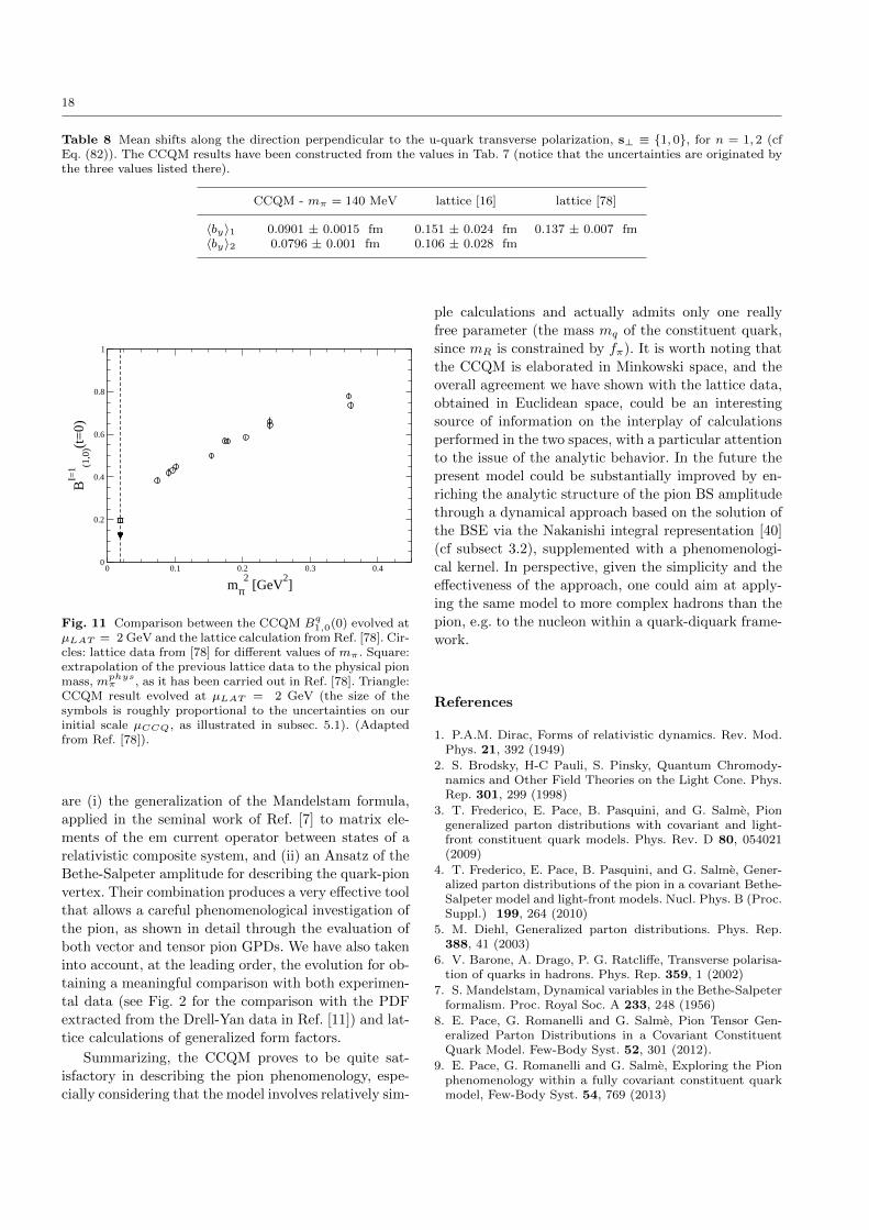
mass appears non trivial. In Fig. 11, a recent lattice

calculation of Bq1,0(t = 0, µLAT ) [78] is compared with

our CCQM (triangles). In general, one has an overall

agreement, a little bit better for Bq2,0(0).

The knowledge of GFFs allows one to investigate

the probability density ρn(b⊥, s⊥) for a transversely-

polarized u-quark (cf Eq. (12)). In particular, one can

address the 3D structure of the pion in the impact pa-

rameter space. For instance, one can calculate the aver-

age transverse shifts when the quark is polarized along

the x-axis, i.e. s⊥ ≡ {1, 0}. The shift for a given n is

n=1

n=2 (x 2)CCQM (n=1)

CCQM(n=2)

Fig. 10 Comparison between the CCQM Bq1,0(t = 0, µLAT )

and Bq2,0(t = 0, µLAT ), divided by mπ and the correspondingresults from the chiral quark model of Ref. [57] and the latticedata of Ref. [16]. Stars: CCQM results evolved at µLAT = 2for Bq1,0(0) (upper one) and for Bq2,0(0) (lower one) (the sizeof the symbols is roughly proportional to the uncertaintieson our initial scale µCCQ as illustrated in subsec. 5.1). Solidlines: results from the chiral quark model of Ref. [57], vs m2

π.Data points: lattice calculations from Ref. [16]. The verticalline corresponds to the physical pion mass. (Adapted fromRef. [57]).

given by [16]

〈by〉n =

∫db⊥ by ρn(b⊥, s⊥)∫db⊥ ρn(b⊥, s⊥)

=1

2mπ

Bqn,0(t = 0)

Aqn,0(t = 0)

(82)

From the CCQM values evolved at µLAT , shown in Tab.

7, one can construct the shifts for n = 1, 2, and then

compare with the corresponding lattice results, as given

in Ref. [16]. In Tab. 8, the comparison is shown (recall

that Aq1,0(t = 0) = 1). Obviously, the same observa-

tions relevant for Tab. 7 can be also repeated for Tab.

8, since it contains the same information but presented

in a different context. The values shown in Tab. 8 in-

dicate that even the simple version of a CCQM is able

to reproduce a distortion of the transverse density in a

direction perpendicular to the quark polarization, and

in turn demonstrate the presence of a non trivial cor-

relation between the orbital angular momenta and the

spin of the constituents inside a pseudoscalar hadron,

that attracts a great interest from both experimental

and theoretical side (see, e.g., [20]).

6 Conclusions

A simple, but fully covariant constituent quark model

has been exploited for investigating the phenomenol-

ogy of the leading-order Generalized Parton Distribu-

tions of the pion. The main ingredients of the approach

18

Table 8 Mean shifts along the direction perpendicular to the u-quark transverse polarization, s⊥ ≡ {1, 0}, for n = 1, 2 (cfEq. (82)). The CCQM results have been constructed from the values in Tab. 7 (notice that the uncertainties are originated bythe three values listed there).

CCQM - mπ = 140 MeV lattice [16] lattice [78]

〈by〉1 0.0901 ± 0.0015 fm 0.151 ± 0.024 fm 0.137 ± 0.007 fm〈by〉2 0.0796 ± 0.001 fm 0.106 ± 0.028 fm

0 0.1 0.2 0.3 0.4

mπ2 [GeV

2]

0

0.2

0.4

0.6

0.8

1

BI=

1 (1,0

)(t=

0)

Fig. 11 Comparison between the CCQM Bq1,0(0) evolved atµLAT = 2 GeV and the lattice calculation from Ref. [78]. Cir-cles: lattice data from [78] for different values of mπ. Square:extrapolation of the previous lattice data to the physical pionmass, mphysπ , as it has been carried out in Ref. [78]. Triangle:CCQM result evolved at µLAT = 2 GeV (the size of thesymbols is roughly proportional to the uncertainties on ourinitial scale µCCQ, as illustrated in subsec. 5.1). (Adaptedfrom Ref. [78]).

are (i) the generalization of the Mandelstam formula,

applied in the seminal work of Ref. [7] to matrix ele-

ments of the em current operator between states of a

relativistic composite system, and (ii) an Ansatz of the

Bethe-Salpeter amplitude for describing the quark-pion

vertex. Their combination produces a very effective tool

that allows a careful phenomenological investigation of

the pion, as shown in detail through the evaluation of

both vector and tensor pion GPDs. We have also taken

into account, at the leading order, the evolution for ob-

taining a meaningful comparison with both experimen-

tal data (see Fig. 2 for the comparison with the PDF

extracted from the Drell-Yan data in Ref. [11]) and lat-

tice calculations of generalized form factors.

Summarizing, the CCQM proves to be quite sat-

isfactory in describing the pion phenomenology, espe-

cially considering that the model involves relatively sim-

ple calculations and actually admits only one really

free parameter (the mass mq of the constituent quark,

since mR is constrained by fπ). It is worth noting that

the CCQM is elaborated in Minkowski space, and the

overall agreement we have shown with the lattice data,

obtained in Euclidean space, could be an interesting

source of information on the interplay of calculations

performed in the two spaces, with a particular attention

to the issue of the analytic behavior. In the future the

present model could be substantially improved by en-

riching the analytic structure of the pion BS amplitude

through a dynamical approach based on the solution of

the BSE via the Nakanishi integral representation [40]

(cf subsect 3.2), supplemented with a phenomenologi-

cal kernel. In perspective, given the simplicity and the

effectiveness of the approach, one could aim at apply-

ing the same model to more complex hadrons than the

pion, e.g. to the nucleon within a quark-diquark frame-

work.

References

1. P.A.M. Dirac, Forms of relativistic dynamics. Rev. Mod.Phys. 21, 392 (1949)

2. S. Brodsky, H-C Pauli, S. Pinsky, Quantum Chromody-namics and Other Field Theories on the Light Cone. Phys.Rep. 301, 299 (1998)

3. T. Frederico, E. Pace, B. Pasquini, and G. Salme, Piongeneralized parton distributions with covariant and light-front constituent quark models. Phys. Rev. D 80, 054021(2009)

4. T. Frederico, E. Pace, B. Pasquini, and G. Salme, Gener-alized parton distributions of the pion in a covariant Bethe-Salpeter model and light-front models. Nucl. Phys. B (Proc.Suppl.) 199, 264 (2010)

5. M. Diehl, Generalized parton distributions. Phys. Rep.388, 41 (2003)

6. V. Barone, A. Drago, P. G. Ratcliffe, Transverse polarisa-tion of quarks in hadrons. Phys. Rep. 359, 1 (2002)

7. S. Mandelstam, Dynamical variables in the Bethe-Salpeterformalism. Proc. Royal Soc. A 233, 248 (1956)

8. E. Pace, G. Romanelli and G. Salme, Pion Tensor Gen-eralized Parton Distributions in a Covariant ConstituentQuark Model. Few-Body Syst. 52, 301 (2012).

9. E. Pace, G. Romanelli and G. Salme, Exploring the Pionphenomenology within a fully covariant constituent quarkmodel, Few-Body Syst. 54, 769 (2013)

19

10. M. Miyama and S. Kumano, Numerical solution of Q2

evolution equations in a brute-force method. Comput. Phys.Commun. 94, 185 (1996)

11. J.S. Conway et al., Experimental study of muon pairsproduced by 252-GeV pions on tungsten. Phys. Rev. D 39,92 (1989)

12. K. Wijesooriya, P. E. Reimer, and R. J. Holt, Pion partondistribution function in the valence region. Phys. Rev. C72, 065203 (2005)

13. D. Brommel, Pion structure from the lattice. Report No.DESY-THESYS-2007-023, 2007

14. D. Brommel, et al (QCDSF/UKQCD Coll.), Quark dis-tributions in the pion. PoS (LATTICE 2007) 140 (2008)

15. D. Brommel et al., Transverse spin structure of hadronsfrom lattice QCD. Prog. Part. Nucl. Phys. 61, 73 (2008)

16. D. Brommel et al., Spin Structure of the pion. Phys. Rev.Lett. 101, 122001 (2008)

17. S. Meißner, A. Metz, M. Schlegel, K. Goeke, General-ized parton correlation functions for a spin-0 hadron. JHEP0808, 038 (2008).

18. Ph. Hagler, Hadron structure from lattice quantum Chro-modynamics. Phys. Rep. 490, 49 (2010)

19. M. Burkardt, Impact parameter dependent parton distri-butions and transverse single spin asymmetries. Phys. Rev.D 72, 094020 (2005) Phys. Rev. D 66, 114005 (2002)

20. M. Burkardt, Transverse deformation of parton distribu-tions and transversity decomposition of angular momen-tum. Phys. Rev. D 72, 094020 (2005)

21. M. Burkardt and B. Hannafious, Are all Boer-Muldersfunctions alike? Phys. Lett. B 658, 130 (2008)

22. M. Diehl and Ph. Hagler, Spin densities in the transverseplane and generalized transversity distributions. Eur. Phys.J. C 44, 87 (2005)

23. D. Brommel et al., The pion form factor from lattice QCDwith two dynamical flavors. Eur. Phys. J. C 51, 335(2007)

24. D. Boer and P. J. Mulders, Time-reversal odd distribu-tion functions in leptoproduction. Phys. Rev. D 57, 5780(1998)

25. Zhun Lu and Bo-Qiang Ma, Nonzero transversity distri-bution of the pion in a quark-spectator-antiquark model.Phys. Rev. D 70, 094044 (2004)

26. A.V. Belitsky, X. Ji and F. Yuan, Final state interactionsand gauge invariant parton distribution. Nucl. Phys. B 656,165 (2003)

27. P. Maris and C. D. Roberts, π and K-meson Bethe-Salpeter amplitudes. Phys. Rev. C 56, 3369 (1997)

28. C. Itzykson and J. B. Zuber, Quantum Field Theory,Dover Pubns., Mineola, NY, 2005

29. J.P.B.C. de Melo, T. Frederico, E. Pace and G. Salme,Pair term in the electromagnetic current within the Front-Form dynamics: spin-0 case. Nucl. Phys. A 707, 399 (2002)

30. J.P.B.C. de Melo, T. Frederico, E. Pace and G. Salme,Electromagnetic form-factor of the pion in the space andtime - like regions within the Front-Form dynamics. Phys.Lett. B 581, 75 (2004)

31. J.P.B.C. de Melo, T. Frederico, E. Pace and G. Salme,Spacelike and timelike pion electromagnetic form-factor andFock state components within the light-front dynamics.Phys. Rev. D 73, 074013 (2006)

32. J.P.B.C. de Melo, T. Frederico, E. Pace, G. Salme andS. Pisano, Timelike and spacelike nucleon electromagneticform factors beyond relativistic constituent quark models.Phys. Lett. B 671,153 (2009)

33. V. N. Gribov, L. N. Lipatov, Deep inelastic e-p scat-tering in perturbation theory. Sov. J. Nucl. Phys. 15, 438(1972) [Yad. Fiz. 15, 781 (1972)]; e+ e- pair annihilationand deep inelastic e p scattering in perturbation theory. 15,675 (1972)

34. G. Altarelli, G. Parisi, Asymptotic freedom in parton lan-guage. Nucl. Phys. B 126, 298 (1977)

35. Yu. L. Dokshitzer, Calculation of the Structure Functionsfor Deep Inelastic Scattering and e+ e- Annihilation byPerturbation Theory in Quantum Chromodynamics. Sov.Phys. JETP 46, 641 (1977)

36. A. V. Efremov, A. V. Radyushkin, Asymptotic behaviorof the pion form factor in quantum chromodynamics. Phys.Lett. B 94, 245 (1980).

37. G. P. Lepage, S. J. Brodsky, Exclusive processes in per-turbative quantum chromodynamics. Phys. Rev. D 22,2157 (1980)

38. R.J. Holt and C.D. Roberts, Nucleon and pion distribu-tion functions in the valence region. Rev. Mod. Phys. 82,2991 (2010)

39. E. P. Biernat, F. Gross, M. T. Pena, and A. Stadler,Pion electromagnetic form factor in the covariant spectatortheory. Phys. Rev. D 89, 016006 (2014)

40. N. Nakanishi, Graph Theory and Feynman Integrals,Gordon and Breach, New York, 1971.

41. J. Carbonell and V.A. Karmanov, Solving Bethe-Salpeterequation in Minkowski space. Eur. Phys. J. A 27, 1 (2006)

42. J. Carbonell and V.A. Karmanov, Solving the Bethe-Salpeter equation for two fermions in Minkowski space. Eur.Phys. J. A 46, 387 (2010)

43. T. Frederico, G. Salme and M. Viviani, Two-body scattering states in Minkowski space andthe Nakanishi integral representation onto thenull plane. Phys. Rev. D 85, 036009 (2012) and\protect\vrule width0pt\protect\href{http://arxiv.org/abs/1112.5568}{arXiv:1112.5568}.

44. T. Frederico, G. Salme and M. Viviani, Quantitativestudies of the homogeneous Bethe-Salpeter equation inMinkowski space. Phys. Rev. D 89, 016010 (2014).

45. T. Frederico, G. Salme and M. Viviani, Solving the in-homogeneous Bethe-Salpeter Equation in Minkowski space:the zero-energy limit. Eur. Phys. J. C 75, 398 (2015).

46. S. M. Dorkin, M. Beyer, S.S. Semikh and L.P. Kaptari,Two-fermion bound states within the Bethe-Salpeter ap-proach. Few-Body Syst. 42, 1 (2008)

47. S. M. Dorkin, L.P. Kaptari, B. Kampfer, Accountingfor the analytical properties of the quark propagator fromthe Dyson-Schwinger equation. Phys. Rev. C 91, 055201(2015).

48. W. Greiner and A. Schaffer. Quantum Chromo Dynam-ics, Springer-Verlag, Berlin (1995)

49. A.V. Belisky and A.V. Radyushkin, Unraveling hadronstructure with generalized parton distributions. Phys. Rep.418, 1 (2005).

50. A.D. Martin et al., Parton distributions for the LHC.Eur. Phys. J. C 63, 189 (2009)

51. X. Ji, Deeply virtual Compton scattering. Phys. Rev. D55, 7114 (1997)

52. P. Hoodbhoy and X. Ji, Helicity-flip off-forward par-ton distributions of the nucleon. Phys. Rev. D 58, 054006(1998).

53. W. Broniowski, E.R. Arriola and K. Golec-Biernat, Gen-eralized parton distributions of the pion in chiral quarkmodels and their QCD evolution. Phys. Rev. D 77, 034023(208)

54. W. Broniowski and E.R. Arriola, Note on the QCD evo-lution of generalized form factors. Phys. Rev. D 79, 057501(2009).

55. N. Kivel and L. Mankiewicz, Conformal string operatorsand evolution of skewed parton distributions. Nucl. Phys.B 557, 271 (1999).

56. M. Kirch, A. Manashov and A. Schafer, Evolution equa-tion for generalized parton distributions. Phys. Rev. D 72,114006 (2005).

20

57. W. Broniowski, A.E. Dorokhov, E.R. Arriola, Transver-sity form factors of the pion in chiral quark models. Phys.Rev. D 82, 094001 (2010)

58. A. E. Dorokhov, W. Broniowski and E. R. Arriola, Gen-eralized quark transversity distribution of the pion in chiralquark models. Phys. Rev. D 84, 074015 (2011)

59. S. Nam and H.C. Kim, Spin structure of the pion fromthe instanton vacuum. Phys. Lett. B 700, 305 (2011)

60. K.A. Olive et al., Particle Data group. Chin. Phys. C 38,090001 (2014)

61. BaBar Collaboration, B. Aubert et al., Measurement ofthe γγ∗ → π0 transition form factor. Phys. Rev. D 80,052002 (2009)

62. Belle Collaboration, S. Uehara et al., Measurement ofγγ∗ → π0 transition form factor at Belle. Phys. Rev. D 86,092007 (2012)

63. S.J. Brodsky, F.-G. Cao and G. F. de Teramond, EvolvedQCD predictions for the meson-photon transition form fac-tors. Phys. Rev. D 84, 033001 (2011)

64. G. P. Lepage and S. J. Brodsky, Exclusive Processes inPerturbative Quantum Chromodynamics. Phys. Rev. D 22,2157 (1980)

65. S.J. Brodsky and G.P. Lepage, Large-angle two-photonexclusive channels in quantum chromodynamics. Phys. Rev.D 24, 1808 (1981)

66. T. D. Rae, Moments of parton distribution amplitudesand structure functions for the light mesons from latticeQCD. ePrint ID: 199359 (2011), http://eprints.soton.ac.uk.

67. S. Capitani, et al (χLF Coll.), Parton distribution func-tions with twisted mass fermions. Phys. Lett. B 639, 520(2006)

68. M. Guagnelli et al (ZeRo Coll.), Non-perturbative pionmatrix element of a twist-2 operator from the lattice. Eur.Phys. J. C 40 69 (2005)

69. A. Abdel-Rehim et al (ETMC Coll.), Nucleon and pionstructure with lattice QCD simulations at physical value ofthe pion. Phys. Rev. D 92, 114513 (2015)

70. W. J. Marciano, Flavor thresholds and Λ in the modifiedminimal-subtraction scheme. Phys. Rev. D 29, 580 (1984)

71. A.D. Martin, W.J. Stirling and R.S. Thorne, MRST par-tons generated in a fixed-flavor scheme. Phys. Lett. B 636,259 (2006)

72. M.B. Hecht, C.D. Roberts and S.M. Schmidt, Valence-quark distributions in the pion. Phys. Rev. C 63, 025213(2001).

73. L. Chang et al, Basic features of the pion valence-quarkdistribution function. Phys. Lett. B 737, 23 (2014)

74. M. Aicher, A. Schafer and W. Vogelsang, Soft-gluon re-summation and valence parton distribution function of thepion. Phys. Rev. Lett. 105, 252003 (2010)

75. W. Broniowski and E. R. Arriola, Gravitational andhigher-order form factors of the pion in chiral quark models.Phys. Rev. D 78, 094011 (2008)

76. W. Broniowski and E.R. Arriola, Application of chi-ral quarks to high-energy processes and lattice QCD.arXiv:0908.4165.

77. M. Diehl and L. Szymanowski, The transverse spin struc-ture of the pion at short distances. Phys. Lett. B 690, 149(2010)

78. I. Baum, V. Lubicz, G. Martinelli, L. Orifici, and S. Sim-ula, Matrix elements of the electromagnetic operator be-tween kaon and pion states. Phys. Rev. D 84, 074503 (2011)

79. J.F. Donoghue and H. Leutwyler, Energy and momentumin chiral theories. Z. Phys. C 52, 343 (1991)