1

The Islamic University of Gaza

Faculty of Engineering

Civil Engineering Department

Hydraulics - ECIV 3322

Chapter 4Part 1

Pipelines and Pipe Networks

2

Introduction

Any water conveying system may include

the following elements:

• pipes (in series, pipes in parallel)

• elbows

• valves

• other devices.

• If all elements are connected in series,

The arrangement is known as a pipeline.

• Otherwise, it is known as a pipe network.

3

How to solve flow problems

• Calculate the total head loss (major and

minor) using the methods of chapter 3

• Apply the energy equation (Bernoulli’s

equation)

This technique can be applied for

different systems.

4

Flow Through A Single Pipe

(simple pipe flow)

• A simple pipe flow: It is a

• flow takes place in one pipe

• having a constant diameter

• with no branches.

• This system may include bends, valves,

pumps and so on.

5

Simple pipe flow

(1)

(2)

6

To solve such system:

• Apply Bernoulli’s equation

• where

pL hhzg

VPz

g

VP 2

2

221

2

11

22

(1)

(2)

g

VK

g

V

D

fLhhh LmfL

22

22

For the same material and constant diameter (same f , same V) we can write:

L

Total

mfL KD

fL

g

Vhhh

2

2

7

ExampleDetermine the difference in the elevations between

the water surfaces in the two tanks which are

connected by a horizontal pipe of diameter 30 cm and

length 400 m. The rate of flow of water through the

pipe is 300 liters/sec. Assume sharp-edged entrance

and exit for the pipe. Take the value of f = 0.032.

Also, draw the HGL and EGL.

Z1 Z

8

Compound Pipe flow

• When two or more pipes with different

diameters are connected together head to

tail (in series) or connected to two common

nodes (in parallel)

The system is called compound pipe flow

9

Flow Through Pipes in Series

• pipes of different lengths and different

diameters connected end to end (in series) to

form a pipeline

10

• Discharge:The discharge through each pipe is the same

• Head loss: The difference in liquid surface levels is equal to the sum

of the total head loss in the pipes:

332211 VAVAVAQ

LBBB

AAA hz

g

VPz

g

VP

22

22

332211 VAVAVAQ

11

LBBB

AAA hz

g

VPz

g

VP

22

22

Hhzz LBA

Where

4

1

3

1 j

mj

i

fiL hhh

g

VK

g

VVK

g

VK

g

VK

g

V

D

Lfh exitenlcent

i

i

i

iiL

22

)(

222

2

3

2

32

2

2

2

13

1

2

12

Flow Through Parallel Pipes

• If a main pipe divides into two

or more branches and again

join together downstream to

form a single pipe, then the

branched pipes are said to be

connected in parallel

(compound pipes).

• Points A and B are called

nodes.

Q1, L1, D1, f1

Q2, L2, D2, f2

Q3, L3, D3, f3

13

• Discharge:

• Head loss: the head loss for each branch is the same

3

1

321

i

iQQQQQ

Q1, L1, D1, f1

Q2, L2, D2, f2

Q3, L3, D3, f3

321 fffL hhhh

g

V

D

Lf

g

V

D

Lf

g

V

D

Lf

222

2

3

3

3

3

2

2

2

22

2

1

1

11

14

ExampleDetermine the flow in each pipe and the main pipe if the head

loss between nodes A and B is 2 m and f=0.01.

Solution

/sm...π

AVQ

m/s.V

.

V

..

g

V.

D

Lf

332

111

1

2

1

2

1

1

1

1015350620404

5062

28192040

25010

22

221 ff hh

/sm.QQQ

/sm...π

Q

m/s.V

.

V

..

g

V.

D

Lf

33

21

332

2

2

2

2

2

2

2

2

10178

1002555720504

5572

8192050

30010

22

15

ExampleThe following figure shows pipe system from cast iron steel.

The main pipe diameter is 0.2 m with length 4m at the end

of this pipe a Gate Valve is fixed as shown. The second pipe

has diameter 0.12 m with length 6.4m, this pipe connected

to two bends R/D = 2.0 and a globe valve. Total Q in the

system = 0.26 m3/s at T=10oC. Determine Q in each pipe at

fully open valves.

16

2

2

031402

20 m.

.πAa

2

2

011302

120 m.

.πAb

ba

babbaa

hh

V.V.VAV A m.

QQQ

0113003140260 3

21

g

V.

g

V

D

Lfh aa

a

aaa

2150

2

22

g

V

g

V.

g

V

D

Lfh bbb

b

bbb

210

21902

2

222

Solution

17

g

V.

.

.f

g

V.

.f b

ba

a2

10380120

46

2150

20

422

22 38103353 15020 bbaa V.f.V.f

0255.0

0185.0

b

a

f

f

22 3810025503353 1500185020 ba V...V..

ba V.V 7194

m/s.V

m/s.V

b

a

6301

6937

V.V.VAV A m. bbbbaa 01130)719.4(03140260 3

/s m...VAQ

/s m...VAQ

bbb

aaa

3

3

0180630101130

2420693703140

by trial and error

18

Example

Determine the flow rate in each pipe (f=0.032).

Also, if the two pipes are replaced with one pipe of the

same length determine the diameter which give the same

flow.

19

20

D

21

Example

Four pipes connected in parallel as shown. The following details are given:

Pipe L (m) D (mm) f

1 200 200 0.020

2 300 250 0.018

3 150 300 0.015

4 100 200 0.020

• If ZA = 150 m , ZB = 144m, determine the discharge in each pipe ( assume PA=PB = Patm)

22

ExampleTwo reservoirs with a difference in water levels of 180 m

and are connected by a 64 km long pipe of 600 mm

diameter and f = 0.015. Determine the discharge through

the pipe. In order to increase this discharge by 50%, another

pipe of the same diameter is to be laid from the lower

reservoir for part of the length and connected to the first

pipe (see figure below). Determine the length of additional

pipe required.

=180mQN QN1

QN2

23

Pipeline with negative Pressure(Siphon phenomena)

• Long pipelines laid to transport water from one reservoir

to another over a large distance usually follow the natural

contour of the land.

• A section of the pipeline may be raised to an elevation

that is above the local hydraulic gradient line (siphon

phenomena) as shown:

24

Definition:

It is a long bent pipe which is used to transfer liquid from a reservoir at a higher elevation to another reservoir at a lower level when the two reservoirs are separated by a hill or high ground

Occasionally, a section of the pipeline may be

raised to an elevation that is above the local HGL.

(siphon phenomena)

25

Siphon happened in the following cases:

• To carry water from one reservoir to another

reservoir separated by a hill or high ground

level.

• To take out the liquid from a tank which is not

having outlet

• To empty a channel not provided with any

outlet sluice.

26

Characteristics of this system

• Point “S” is known as the summit.

• All Points above the HGL have pressure less than atmospheric (negative value)

• If the absolute pressure is used then the atmospheric absolute pressure = 10.33 m

• It is important to maintain pressure at all points (above HGL) in a pipeline above the vapor pressure of water (not be less than zero Absolute )

27

LS

Sp

LSSS

p

pp

hP

ZZ

hZP

g

VZ

P

g

V

22

22

A S

-ve value Must be -ve value ( below the atmospheric pressure)

Negative pressure exists in the pipelines wherever the pipe line is raised above the

hydraulic gradient line (between P & Q)

Sp VV

28

The negative pressure at the summit point can reach

theoretically to -10.33 m water head (gauge pressure) and

zero (absolute pressure). But in the practice water

contains dissolved gasses that will vaporize before -10.33

m water head which reduces the pipe flow cross section.

Generally, this pressure reach to -7.6 m water head (gauge

pressure) and 2.7 m (absolute pressure)

In practice…

29

ExampleSiphon pipe between two tanks and pipe has diameter of

20 cm and length 500 m as shown. The difference

between reservoir levels is 20 m. The distance between

reservoir A and summit point S is 100 m. Calculate the

flow in the system and the pressure head at summit.

f=0.02

3m

20m

30

Solution

31

• Pumps may be needed in a pipeline to lift water from a lower elevation or simply to boost the rate of flow. Pump operation adds energy to water in the pipeline by boosting the pressure head

• The computation of pump installation in a pipeline is usually carried out by separating the pipeline system into two sequential parts, the suction side and discharge side.

Pumps

32

LsRP hHHH

See example 4.5

Pumps selection will

be discussed in details

in next chapters

33

Branching in pipes occur when water is brought by pipes to a

junction when more than two pipes meet.

This system must simultaneously satisfy two basic conditions:

1 – The total amount of water brought by pipes to a junction must

equal to that carried away from the junction by other pipes.

2 – All pipes that meet at the junction must share the same pressure

at the junction. Pressure at point J = P

Branching pipe systems

0Q

34

Three-reservoirs problem

(Branching System)

How we can demonstrate the

hydraulics of branching pipe System??

by the classical three-reservoirs problem

35

This system must satisfy:

Q3 = Q1 + Q2

2) All pipes that meet at junction “J” must

share the same pressure at the junction.

1) The quantity of water brought to junction “J” is equal

to the quantity of water taken away from the junction:

Flow Direction????

36

Types of three-reservoirs problem:

Type 1:

• given the lengths, diameters, and materials of all pipes involved

D1 , D2 , D3 , L1 , L2 , L3 , and e or f

• given the water elevation in each of the three reservoirs

Z1 , Z2 , Z3

• determine the discharges to or from each reservoir,

Q1 , Q2 and Q3

Two types

This types of problems are most conveniently

solved by trial and error

37

• First assume a piezometric surface elevation, P , at the junction.

• This assumed elevation gives the head losses hf1, hf2, and hf3

• From this set of head losses and the given pipe diameters, lengths, and material, the trial computation gives a set of values for discharges Q1 , Q2 ,and Q3 .

• If the assumed elevation P is correct, the computed Q’s should satisfy:

• Otherwise, a new elevation P is assumed for the second trial.

• The computation of another set of Q’s is performed until the above condition is satisfied.

Q Q Q Q 1 2 3 0

38

Note:

• It is helpful to plot the computed trial values of P

against ΣQ.

• The resulting difference may be either plus or minus

for each trial.

• However, with values obtained from three trials, a

curve may be plotted as shown in the next example.

The correct discharge is indicated by the

intersection of the curve with the vertical axis.

39

Example

AJBJCJPipe

100040002000Length m

305040Diameter cm

0.0240.0210.022f

In the following figure determine the flow in each pipe

40

Trial 1

ZP= 110m

Applying Bernoulli Equation between A , J :

g

V

g

V

D

LfZZ PA

23.0

1000024.0110120

2.

2

1

2

1

1

1

1

V1 = 1.57 m/s , Q1 = 0.111 m3/s

g

V

g

V

D

LfZZ BP

25.0

4000021.0100110

2.

2

2

2

2

2

2

2

V2 = 1.08 m/s , Q2 = - 0.212 m3/s

Applying Bernoulli Equation between B , J :

41

g

V

g

V

D

LfZZ CP

24.0

2000022.080110

2.

2

3

2

3

3

3

3

Applying Bernoulli Equation between C , J :

V3 = 2.313 m/s , Q2 = - 0.291 m3/s

0392.0291.0212.0111.0321 QQQQ

42

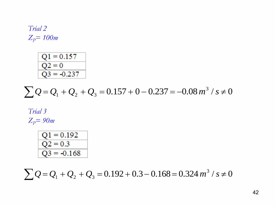
Trial 2

ZP= 100m

0/ 08.0237.00157.0 3

321 smQQQQ

Trial 3

ZP= 90m

0/ 324.0168.03.0192.0 3

321 smQQQQ

43

Draw the relationship between and PQ

99m Pat 0 Q

44

Type 2:

• Given the lengths , diameters, and materials of all pipes involved;

D1 , D2 , D3 , L1 , L2 , L3 , and e or f

• Given the water elevation in any two reservoirs,

Z1 and Z2 (for example)

• Given the flow rate from any one of the reservoirs,

Q1 or Q2 or Q3

• Determine the elevation of the third reservoir Z3 (for example) and the rest of Q’s

This types of problems can be solved by simply using:

• Bernoulli’s equation for each pipe

• Continuity equation at the junction.

45

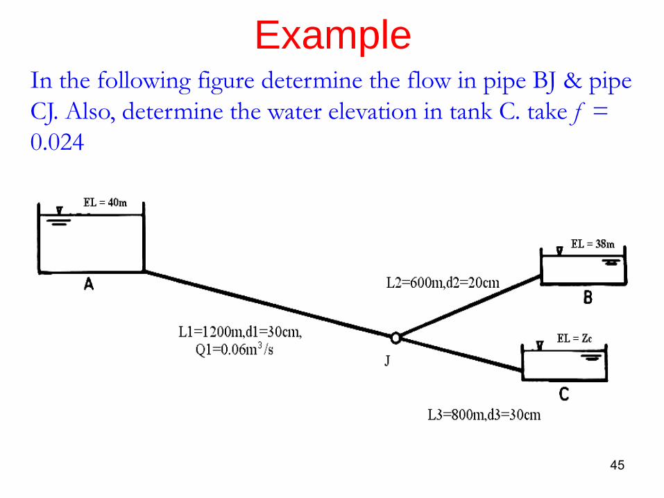
Example In the following figure determine the flow in pipe BJ & pipe

CJ. Also, determine the water elevation in tank C. take f =

0.024

46

m.Z

.

.

..Z

g

V.

D

LfZZ

m/s.

.π

.

A

QV

P

PPA

47536

8192

8490

30

1200024040

2

8490

304

060

22

1

1

11

21

11

Solution

/sm 0.0203Q0.645m/sV

9.812

V

0.2

6000.02436.47538

2g

V.

D

LZZ

3

22

2

2

2

2

2

22PB

f

Applying Bernoulli Equation between B , J :

Applying Bernoulli Equation between A , J :

47

mZ

gg

V

D

LfZZ

c

CP

265.32

2

136.1

3.0

800024.0 Z- 6.4753

2.

2

c

2

3

3

33

Applying Bernoulli Equation between C , J :

smQQQ

QQQQ

/ 0803.00203.006.0

0

3

213

321

sm

A

QV / 136.1

3.04

0803.0

23

3

3

48

Group Work

ACAB

ACAB

BDBC

BDBCAB

VV

VV

QQ

QQQ

125.1

3.024.0

0

2

4

2

4

smQsmV

smQQsmV

VV

VV

g

V

g

V

hh

ABAB

BDBCBC

BCBC

BCAB

ABAB

BCAB

/31.0/5.2

/155.0/2.2

10 816.0)125.1(55.2

10 7.155.2

1023.0

100001.0

24.0

200001.0

10

3

3

22

22

01.0f

Find the flow in each pipe

VBC

2

49

Power Transmission Through Pipes

• Power is transmitted through pipes by the

water (or other liquids) flowing through them.

• The power transmitted depends upon:(a) the weight of the liquid flowing through the pipe

(b) the total head available at the end of the pipe.

50

• What is the power available at the end B of

the pipe?

• What is the condition for maximum

transmission of power?

51

Total head (energy per unit weight) H of fluid is

given by:

time

Weightx

weight

Energy

time

EnergyPower

ZP

g

VH

2

2

QQgtime

Weight

Therefore:

Power Q H

Units of power:

N . m/s = Watt

745.7 Watt = 1 HP (horse power)

52

For the system shown in figure, the following can be stated:

mf

m

f

hhHγ Q

γ Q h

γ Q h

γ Q H

PowerExit At

lossminor todue dissipatedPower

friction todue dissipatedPower

Power EntranceAt

53

Condition for Maximum Transmission of Power:

The condition for maximum transmission of power occurs when : 0dV

dP

][ mf hhHQP

Neglect minor losses and use VDAVQ ]4

[ 2

So ]2

[4

32

g

V

D

LfHVDP

0]2

3[

4

22 VDg

fLHD

dV

dP

fhg

V

D

fLH 3

23

2

3

Hh f

Power transmitted through a pipe is maximum when the loss of head due

of the total head at the inlet 3

1

to friction equal

54

Maximum Efficiency of Transmission of Power:

Efficiency of power transmission is defined as

inlet at the suppliedPower

outlet at the availablePower

H

hhH

QH

hhHQ mfmf ][][

or

H

hH f ][

Maximum efficiency of power transmission occurs when3

Hh f

%67.663

2]

3[

max

H

HH

(If we neglect minor losses)

55

ExamplePipe line has length 3500m and Diameter 0.3m is used to

transport Power Energy using water. Total head at entrance

= 500m. Determine the maximum power at the Exit. f =

0.024

fout h Hγ QP

mH

h f3

500

3at Power Max.

g

V

..

g

V

D

Lfh f

230

35000240

2

22

m/s 3.417V

/s m...AVQ π 32

424150417330

56

HP.

tt) N.m/s (Wa

..

HgQ

HHgQ

hHγQP f

10597745

789785789785

500241508191000

3

32

32