ABSTRACTBottom-up program analysis has been traditionally easy to par-
allelize because functions without caller-callee relations can be
analyzed independently. However, such function-level parallelism
is significantly limited by the calling dependence - functions with
caller-callee relations have to be analyzed sequentially because
the analysis of a function depends on the analysis results, a.k.a.,
function summaries, of its callees.We observe that the calling depen-
dence can be relaxed in many cases and, as a result, the parallelism
can be improved. In this paper, we present Cheetah, a framework
of bottom-up data flow analysis, in which the analysis task of each
function is elaborately partitioned into multiple sub-tasks to gener-
ate pipelineable function summaries. These sub-tasks are pipelined
and run in parallel, even though the calling dependence exists. We
formalize our idea under the IFDS/IDE framework and have im-
plemented an application to checking null-dereference bugs and
taint issues in C/C++ programs. We evaluate Cheetah on a series
of standard benchmark programs and open-source software sys-
tems, which demonstrates significant speedup over a conventional
parallel design.
CCS CONCEPTS• Software and its engineering → Software verification andvalidation.KEYWORDSCompositional program analysis, modular program analysis, bottom-
up analysis, data flow analysis, IFDS/IDE.
ACM Reference Format:Qingkai Shi and Charles Zhang. 2020. Pipelining Bottom-up Data Flow
Analysis. In 42nd International Conference on Software Engineering (ICSE’20), May 23–29, 2020, Seoul, Republic of Korea. ACM, New York, NY, USA,
13 pages. https://doi.org/10.1145/3377811.3380425
1 INTRODUCTIONBottom-up analyses work by processing the call graph of a program
upwards from the leaves – before analyzing a function, all its callee
functions are analyzed and summarized as function summaries [4, 8,
9, 11, 15, 16, 54, 63, 64]. These analyses have two key strengths: the
Permission to make digital or hard copies of all or part of this work for personal or
classroom use is granted without fee provided that copies are not made or distributed
for profit or commercial advantage and that copies bear this notice and the full citation
on the first page. Copyrights for components of this work owned by others than ACM
must be honored. Abstracting with credit is permitted. To copy otherwise, or republish,
to post on servers or to redistribute to lists, requires prior specific permission and/or a
Figure 1: Conventional parallel design of bottom-up pro-gram analysis. Each rectangle represents the analysis taskfor a function.
time
f0
h0
f1
h1
f2
h2
g0 g1 g2
Figure 2: The analysis task of each function is partitionedinto multiple sub-tasks. All sub-tasks are pipelined.
function summaries they compute are highly reusable and they are
easy to parallelize because the analyses of functions are decoupled.
While almost all existing bottom-up analyses take advantage of
such function-level parallelization, there is little progress in improv-
ing its parallelism. As reported by recent studies, it still needs to
take a few hours, even tens of hours, to precisely analyze large-scale
software. For example, it takes 6 to 11 hours for Saturn [64] and
Calysto [4] to analyze programs of 685KLoC [4]. It takes about 5
hours for Pinpoint [54] to analyze about 8 million lines of code.
With regard to the performance issues, McPeak et al. [35] pointed
out that the parallelism often drops off at runtime and, thus, the
CPU resources are usually not well utilized. Specifically, this is
because the parallelism is significantly limited by the calling depen-dence – functions with caller-callee relations have to be analyzed
sequentially because the analysis of a caller function depends on the
analysis results, i.e., function summaries, of its callee functions. To
illustrate this phenomenon, let us consider the call graph in Figure 1
where the function f calls the functions, g and h. In a conventional
bottom-up analysis, only functions without caller-callee relations,
e.g., the function g and the function h, can be analyzed in parallel.
The analysis of the function f cannot start until the analyses of thefunctions, g and h, complete. Otherwise, when analyzing a call site
of the function, g or h, in the function f, we may miss some effects
of the callees due to the incomplete analysis.1
1This is different from a top-down method that can let the analysis of the function frun first but stop to wait for the analysis results of the function g when analyzing a
ICSE ’20, May 23–29, 2020, Seoul, Republic of Korea Qingkai Shi and Charles Zhang
In this paper, we present Cheetah, a framework of bottom-up
data flow analysis that breaks the limits of function boundaries,
so that functions having calling dependence can be analyzed in
parallel. As a result, we can achieve much higher parallelism than
the conventional parallel design of bottom-up analysis. Our key
insight is that many analysis tasks of a caller function only depend
on partial analysis results of its callee functions. Thus, the analysis
of the caller function can start before the analyses of its callee
functions complete. Therefore, our basic idea is to partition the
analysis task of a function into multiple sub-tasks, so that we can
pipeline the sub-tasks to generate function summaries. The key to
the partition is a soundness criterion, which requires a sub-task
only depends on the summaries produced by the sub-tasks finished
in the callees. Violating this criterion will cause the analysis to
neglect certain function effects and make the analysis unsound.
To illustrate, assume that the analysis task of each function in
Figure 1, e.g., the function f, is partitioned into three sub-tasks,
f0, f1, and f2, each of which generates one kind of function sum-
maries. These sub-tasks satisfy the constraints that the sub-task
fi only depends on the function summaries produced by the sub-
task gj and the sub-task hj (j ≤ i). As a result, these sub-tasks canbe pipelined as illustrated in Figure 2, where the analysis of the
function f starts immediately after the sub-tasks g0and h0 finish.
Clearly, the parallelism in Figure 2 is much higher than that in
Figure 1, providing a significant speedup over the conventional
parallel design of bottom-up analysis.
In this paper, we formalize our idea under the IFDS/IDE frame-
work for a wide range of data flow problems known as the inter-
procedural finite distributive subset or inter-procedural distributive
environment problems [45, 50]. In both problems, the data flow
functions are required to be distributive over the merge operator.
Although this is a limitation in some cases, the IFDS/IDE frame-
work has been widely used for many practical problems such as
secure information flow [3, 23, 42], typestate [19, 39], alias sets [40],
specification inference [55], and shape analysis [47, 65]. Given any
of those IFDS/IDE problems, conventional solutions compute func-
tion summaries either in a bottom-up fashion (e.g., [49, 67]) or in a
top-down manner (e.g., [45, 50]), depending on their specific design
goals. In this paper, we focus on the bottom-up solutions and aim to
improve their performance via the pipeline parallelization strategy.
We implemented Cheetah to path-sensitively check null derefer-
ences and taint issues in C/C++ programs. Our evaluation of Chee-tah is based on standard benchmark programs and many large-scale
software systems, which demonstrates that the calling dependence
significantly limits the parallelism of bottom-up data flow analy-
sis. By relaxing this dependence, our pipeline strategy achieves
2×-3× speedup over the conventional parallel design of bottom-
up analysis. Such speedup is significant enough to make many
overly lengthy analyses useful in practice. In summary, the main
contributions of this paper include the following:
• We propose the design of pipelineable function summaries,
which enables the pipeline parallelization strategy for bottom-
up data flow analysis.
• We formally prove the correctness of our approach and apply
it to a null analysis and a taint analysis to show its general-
izability.
id: λS.S f: λS.a g: λS. if a ∈ S : (S ∪ b) else (S – b)
0 a b
0 a b
.
.
..
. .
0 a b
0 a b
.
.
..
. .
0 a b
0 a b
.
.
..
. .
Figure 3: Data flow functions and their representation in theexploded super-graph [45].
• We conduct a systematic evaluation to demonstrate that we
can achieve much higher parallelism and, thus, run faster
than the state of the arts.
2 BACKGROUND AND OVERVIEWIn this section, we introduce the background of the IFDS/IDE frame-
work (Section 2.1) and provide an example to illustrate how we
improve the parallelism of a bottom-up analysis by partitioning the
analysis of a function (Section 2.2).
2.1 The IFDS/IDE FrameworkThe IFDS/IDE framework aims to solve a wide range of data flow
problems known as Inter-procedural Finite Distributive Subset or
Inter-procedural Distributive Environment problems [45, 50]. Its
basic idea is to transform a data flow problem to a graph reachability
problem on the exploded super-graph, which is built based on the
inter-procedural control flow graph of a program.
The IFDS Framework. In the IFDS framework, every vertex
(si ,d) in the exploded super-graph stands for a statically decidable
data flow fact, or simply, fact, d at a program point si . Every edge
models the data flow functions between data flow facts. In the
paper, to ease the explanation, we use si to denote the program
point at Line i in the code. For example, in an analysis to check
null dereference, the vertex (si ,d) could denote that the variable dis a null pointer at Line i . As for the edges or data flow functions,
Figure 3 illustrates three examples that show how the commonly-
used data flow functions are represented as edges in the exploded
super-graph. The vertices at the top are the data flow facts before a
program point and the vertices at the bottom represent the facts
after the program point.
The first data flow function id is the identity function which
maps each data flow fact before a program point to itself. It indicates
that the statement at the program point has no impacts on the data
flow analysis.
The special vertex for the fact 0 is associated with every programpoint in the program. It denotes a tautology, a data flow fact that
always holds. An edge from the fact 0 to a non-0 fact indicates
that the non-0 fact is freshly created. For example, in the second
function in Figure 3, the fact a is created, which is represented by
an edge from the fact 0 to the fact a. At the same time, since a is theonly fact after the data flow function, there is no edge connecting
the fact b before and after the program point.
2
Pipelining Bottom-up Data Flow Analysis ICSE ’20, May 23–29, 2020, Seoul, Republic of Korea
14. bool y = …;15.
16. int* bar(int* a) 17.
18. int* b = null;19.
20. …21.
22. int* c = y ? a : b;23.
24. return c;25.
26.
1. …2.
3. int* foo() 4.
5. int* p = bar(null);6.
7. int* q = p;8.
9. int* r = q;10.
11. return r;12.
13.
. . . .
. . . .
. . . .
. . . .
. . . .
0 q r p
. . . .
. . . .
. . . .
. . . .
. . . .
0 b c a
normal flow function call flow function return flow function
to callers
Figure 4: An example of the exploded super-graph for a null-dereference analysis.
The third data flow function is a typical function that models
the assignment b = a. In the exploded super-graph, the variable ahas the same value as before. Thus, there is an edge from the data
flow fact a to itself. The variable b gets the value from the variable
a, which is modeled by the edge from the fact a to the fact b.It is noteworthy that the data flow facts are not limited to simple
values like the local variables in the examples of the paper. For
example, in alias analysis, the facts can be sets of access paths [59].
In typestate analysis, the facts can be the combination of different
typestates [39].
Figure 4 illustrates the exploded super-graph for a data flow
analysis that tracks the propagation of null pointers. Since Line 18
assigns a null pointer to the variable b, we have the edge from the
vertex (s17, 0) to the vertex (s19, b), meaning that we have the data
flow fact b = null at Line 19. Since Line 19 does not change the
value of the variable a, we have the edge from the vertex (s17, a)to the vertex (s19, a), which means the data flow fact about the
variable a does not change.
Assuming that smain is the program entry point, the IFDS frame-
work aims to find paths, or determine the reachability relations,
between the vertex (smain, 0) and the vertices of interests. Each of
such paths represents that some data flow fact holds at a program
point. For instance, the path from the vertex (s4, 0) to the vertex
(s12, r) in Figure 4 implies that the fact r = null holds at Line 12.
The IFDS method is efficient because it computes function sum-
maries only once for each function. Each summary is a path on the
exploded super-graph connecting a pair of vertices at the entry and
the exit of a function. The path from the vertex (s17, a) to the vertex(s25, c) in Figure 4 is such a summary of the function bar. When
analyzing the callers of the function bar, e.g., the function foo, wecan directly jump from the vertex (s4, 0) to the vertex (s6,p) usingthe summary without analyzing the function bar again.
The IDE Framework. The IDE framework is a generalization
of the IFDS framework [50]. Similar to the IFDS framework, it also
works as a graph traversal on an exploded super-graph. There are
three major differences. First, each vertex on the exploded super-
graph is no longer associated with a simple data flow fact d, but an
environment mapping a fact d to a value v from a separate value
domain, denoted as d 7→ v. Second, due to the first difference, thedata flow functions, i.e., the edges on the exploded super-graph,
transform an environment d 7→ v to the other d′ 7→ v′. Thethird important difference is that each edge on the exploded super-
graph is labeled with an environment transform function, which
makes IDE no longer only a simple graph reachability problem.
Instead, it has to find the paths between two vertices of interests
and, meanwhile, compose the environment transform functions
labeled on the edges along the paths. These differences widen the
class of problems that can be expressed in the IFDS framework.
In this paper, for simplicity, we describe our work under the IFDS
framework. This does not lose the generality for the IDE problems
because, intuitively, both problems are solved by a graph traversal
on the exploded super-graph.
2.2 Cheetah in a NutshellLet us briefly explain our approach using the example in Figure 4,
where the analysis aims to track the propagation of null pointers.
Bottom-up Analysis. For the example in Figure 4, a conven-
tional bottom-up analysis firstly analyzes the function bar andproduces function summaries to summarize its behavior. With the
function summaries in hand, the function foo then is analyzed.
Using the symbol to denote a path between two vertices, a
common IFDS/IDE solution will generate the following two intra-
procedural paths as the summaries of the function bar:
• The path (s17, a) (s25, c) summarizes the function behav-
ior that a null pointer created in a caller of the function bar,i.e., a = null, may be returned back to the caller.
• The path (s17, 0) (s25, c) summarizes the function behav-
ior that a null pointer created in the function bar may be
returned to the caller functions.
Note that we do not need to summarize the path (s17, 0) (s25, 0) for the function bar, because the fact 0 is a tautology and
always holds.
3
ICSE ’20, May 23–29, 2020, Seoul, Republic of Korea Qingkai Shi and Charles Zhang
• (s17, 0)⤳(s25, c)
time
• (s17, a)⤳(s25, c)
• (s4, 0)⤳(s17, a)⤳(s25, c)⤳(s6, p)⤳(s10, r)
• (s4, 0)⤳(s17, 0)⤳(s25, c)⤳(s6, p)⤳(s10, r)
analyzing the function bar
analyzing the function foo
foo1 foo2
bar0 bar1
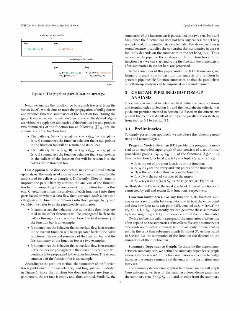
Figure 5: The pipeline parallelization strategy.
Next, we analyze the function foo by a graph traversal from the
vertex (s4, 0), which aims to track the propagation of null pointers
and produce function summaries of the function foo. During the
graph traversal, when the call flow functions (i.e., the dashed edges)
are visited, we apply the summaries of the function bar and producetwo summaries of the function foo as following (J·Kbar are the
summaries of the function bar):
• The path (s4, 0) J(s17, a) (s25, c)Kbar (s6,p) (s12, r) summarizes the function behavior that a null pointer
in the function foo will be returned to its callers.
• The path (s4, 0) J(s17, 0) (s25, c)Kbar (s6,p) (s12, r) summarizes the function behavior that a null pointer
in the callees of the function foo will be returned to the
callers of the function foo.
Our Approach. As discussed before, in a conventional bottom-
up analysis, the analysis of a caller function needs to wait for the
analysis of its callees to complete. Differently, Cheetah aims to
improve the parallelism by starting the analysis of the function
foo before completing the analysis of the function bar. To this
end, Cheetah partitions the analysis of each function f into three
parts based on where a data flow fact is created. Such a partition
categorizes the function summaries into three groups, f0, f1, andf2, which we refer to as the pipelineable summaries:
• f0 summarizes the behavior that some data flow facts cre-
ated in the caller functions will be propagated back to the
callers through the current function. The first summary of
the function bar is an example.
• f1 summarizes the behavior that some data flow facts created
in the current function will be propagated back to the caller
functions. The second summary of the function bar and the
first summary of the function foo are two examples.
• f2 summarizes the behavior that some data flow facts created
in the callees are propagated to the current function and will
continue to be propagated to the caller functions. The second
summary of the function foo is an example.
According to the partitionmethod, the summaries of the function
foo is partitioned into two sets, foo1 and foo2, just as illustratedin Figure 5. Since the function foo does not have any function
parameters, the set foo0 is empty and, thus, omitted. Similarly, the
summaries of the function bar is partitioned into two sets, bar0 andbar1. Since the function bar does not have any callees, the set bar2is empty and, thus, omitted. As detailed later, the above partition is
sound because it satisfies the constraint that summaries in the set
fooi only depends on the summaries in the set barj (j ≤ i ). Thus,we can safely pipeline the analyses of the function foo and the
function bar - we can start analyzing the function foo immediately
after summaries in the set bar0 are generated.
In the remainder of this paper, under the IFDS framework, we
formally present how to partition the analysis of a function to
generate pipelineable function summaries, so that the parallelism
of bottom-up analysis can be improved in a sound manner.
3 CHEETAH: PIPELINED BOTTOM-UPANALYSIS
To explain our method in detail, we first define the basic notations
and terminologies in Section 3.1 and then explain the criteria that
guide our partition method in Section 3.2. Based on the criteria, we
present the technical details of our pipeline parallelization strategy
from Section 3.3 to Section 3.5.
3.1 PreliminariesTo clearly present our approach, we introduce the following nota-
tions and terminologies.
Program Model. Given an IFDS problem, a program is mod-
eled as an exploded super graph G that consists of a set of intra-
procedural graphs Gf,Gg,Gh . . . of the functions f, g, h, . . . .Given a function f, its local graph Gf is a tuple (Lf, ef,xf,Df,Ef):
• Lf is the set of program locations in the function.
• ef,xf ∈ Lf are the entry and exit points of the function.
• Df is the set of data flow facts in the function.
• Lf × Df is the set of vertices of the graph.
• Ef ⊆ (Lf × Df) × (Lf × Df) is the edge set (see Figure 3).
As illustrated in Figure 4, the local graphs of different functions are
connected by call and return flow functions, respectively.
Function Summaries. For any function f, its function sum-
maries are a set of paths between data flow facts at the entry point
and data flow facts at its exit point [45], denoted as Sf = (ef , a) (xf , b) : a, b ∈ Df . Apparently, we can generate these summaries
by traversing the graph Gf from every vertex at the function entry.
Owing to function calls in a program, the summaries of a function
often depend on the summaries of its callees. We say a summary set
S depends on the other summary set S ′ if and only if there exists a
path in the set S that subsumes a path in the set S ′. As illustratedin Section 2.2, the summaries of the function foo depend on the
summaries of the function bar.
Summary Dependence Graph. To describe the dependence
between summary sets, we define the summary dependence graph,
where a vertex is a set of function summaries and a directed edge
indicates the source summary set depends on the destination sum-
mary set.
The summary dependence graph is built based on the call graph.
Conventionally, vertices of the summary dependence graph are
the summary sets Sf, Sg, Sh . . . , and an edge from the summary
4
Pipelining Bottom-up Data Flow Analysis ICSE ’20, May 23–29, 2020, Seoul, Republic of Korea
set Sf to the summary set Sg exists if and only if the function fcalls the function g. A bottom-up analysis works by processing
the summary dependence graph upwards from the leaves. It starts
generating summaries in a summary set if it does not depend on
other summary sets or the summary sets it depends on have been
generated. Summary sets that do not have dependence relations
can be generated in parallel.
Problem Definition. In this paper, we aim to find a partition
for the summary set of each function, say Π(Sf ) = S0
f , S1
f , S2
f , . . . ,2
such that a vertex of the summary dependence graph is no longer
a complete summary set Sf but a subset Sif (i ≥ 0). Meanwhile,
to improve the parallelism, the bottom-up analysis based on the
dependence graph should be able to generate summaries for a pair
of caller and callee functions at the same time. In detail, the partition
needs to satisfy the criteria discussed in the next subsection.
3.2 Partition CriteriaGiven a pair of functions where the function f calls the function g,we use the set Ω(Sf , Sg) ⊆ Π(Sf ) ×Π(Sg) to denote the dependencerelations between summary sets. Generally, an effective partition
method must meet the following criteria to improve the parallelism
of a bottom-up analysis.
The Effectiveness Criterion. This criterion concerns whether
the dependence between summary sets in the conventional bottom-
up analysis is actually relaxed, so that the parallelism can be im-
proved. We say the partition is effective if and only if |Ω(Sf , Sg) | <|Π(Sf ) × Π(Sg) |. Intuitively, this means that some summaries in
the caller function do not depend on all summaries in callee func-
tions. Thus, the dependence relation in the conventional bottom-up
analysis is relaxed.
The Soundness Criterion. This criterion concerns the correct-
ness after the dependence between summary sets is relaxed. We say
the partition is sound if and only if the following condition is sat-
isfied: if the set Sif depends on the set Sjg, then (Sif , S
jg) ∈ Ω(Sf , Sg).
Violating this criterion will cause the analysis to neglect certain
function summaries and make the analysis unsound.
The Efficiency Criterion. This criterion concerns how many
computational resources we need to consume in order to determine
how to partition a summary set. Since summaries in the summary
sets, Sf and Sg, are unknown before an analysis completes, the exact
dependence relations between summaries in the two sets are also
undiscovered. This fact makes it difficult to perform a fine-grained
partition, unless the analysis has been completed and we have
known what summaries are generated for each function.
As a trade-off, conventional bottom-up analysis does not parti-
tion the summary sets (or equivalently, Π(Sf ) = Sf and Π(Sg) =Sg). It conservatively utilizes the observation that all summaries
in the set Sf may depend on certain summaries in the set Sg, i.e.,Ω(Sf , Sg) = (Sf , Sg). Such a conservative method satisfies the
soundness criterion and does not partition the summary sets. How-
ever, apparently, it does not meet the effectiveness criterion because
|Ω(Sf , Sg) | = |Π(Sf ) × Π(Sg) | = 1.
2A set partition needs to satisfy ∪i≥0S if = Sf and ∀i, j ≥ 0 : S if ∩ S
jf = ∅.
3.3 Pipelineable Summary-Set PartitionGenerally, it is challenging to partition a summary set satisfying
the above criteria because the exact dependence between sum-
maries are unknown before the summaries are generated. We now
present a coarse-grained partition method that requires few pre-
computations, and thus, meets the efficiency criterion. Meanwhile,
it also meets the effectiveness and soundness criteria and, thus, can
soundly improve the parallelism of a bottom-up analysis. We also
establish a few lemmas to prove the correctness of our approach.
Intuitively, given a summary set Sf , we partition it according to
where a data flow fact is created: in a caller of the function f, inthe current function f, and in a callee of the function f. Formally,
Π(Sf ) = S0
f , S1
f , S2
f , where
S0f = (ef , a) (xf , b) : a , 0
S1f = (ef , 0) (eg, a) (xf , b) : f = g ∨ a , 0
S2f = (ef , 0) (eg, 0) (xf , b) : f , gBy definition, there is no edge from a non-0 data flow fact to
the fact 0 on the exploded super-graph. An edge from the fact 0to a non-0 fact means that the non-0 fact is freshly created [45].
Thus, any summary path in the set S0f does not go through the
fact 0, meaning that the data flow fact is created in a caller of the
function f. On the other hand, since a summary path in the set S1for the set S2f starts with the fact 0, it means that the non-0 data
flow fact on the summary path must be created in the function f ora callee of the function f. Specifically, since a summary path in the
set S1f does not go through the fact 0 in callee functions, the non-0data flow fact on the summary path is created in the function f.Similarly, the non-0 data flow fact on a path from the set S2f must
be created in a callee of the function f.The following lemma states that generating summaries in the
sets, S0f , S1
f , and S2
f , does not miss any summary in the set Sf and,meanwhile, does not repetitively generate a summary in the set Sf .
Lemma 3.1.
⋃i≥0 S
if = Sf and ∀i, j ≥ 0 : Sif ∩ S
jf = ∅.
Proof. This follows the definitions of the sets S0f , S1
f , and S2
f .
Next, we study whether such a partition method follows the
effectiveness and soundness criteria. The key to the problem is to
compute the set Ω(Sf , Sg) of dependence relations between a pair
of summary sets, Sif and Sjg, given any pair of caller-callee functions,
f and g.
Lemma 3.2. The sets S0f , S1
f , and S2
f depend on the set S0g .
Proof. This follows the fact that any summary path in a caller
function may go through a callee’s summary path and the set S0g is
a part of the callee’s summaries.
Lemma 3.3. The set S2f depends on the sets S1g and S2
g .
Proof. By definition, a summary path in the set S2f needs to go
through the vertex (eg, 0). Given the function g, summary paths
in both the set S1g and the set S2g start with the vertex (eg, 0). Thus,the set S2f depends on the sets S1g and S
2
g .
To demonstrate that the above lemmas do not miss any depen-
dence relations, we establish the following two lemmas.
5
ICSE ’20, May 23–29, 2020, Seoul, Republic of Korea Qingkai Shi and Charles Zhang
S 0f S1f S2f
S 0g S1g S2g
Figure 6: The summary dependence graph for a caller-calleefunction pair, f and g.
Lemma 3.4. The set S0f does not depend on the sets S1g and S2
g .
Proof. This follows the fact that a non-0 data flow fact cannot
be connected back to the fact 0 [45], but a summary path in the
sets S1g and S2
g must start with the fact 0.
Lemma 3.5. The set S1f does not depend on the sets S1g and S2
g .
Proof. By definition, a summary path in the set S1f does not go
through the fact 0 in a callee function. However, a summary path
in the sets S1g and S2g must start with the fact 0. Thus, the set S1fdoes not depend on the sets S1g and S
2
g .
Putting Lemma 3.2 to Lemma 3.5 together, we have the depen-
dence set Ω(Sf , Sg) = (S0
f , S0
g ), (S1
f , S0
g ), (S2
f , S0
g ), (S2
f , S1
g ), (S2
f , S2
g ),
which does not miss any dependence relation between the set Sifand the set S
jg. Thus, the partition method satisfies the soundness
the effectiveness criterion is satisfied, meaning that the dependence
between the summary sets is relaxed and, based on the partition,
the parallelism of a bottom-up analysis can be improved.
Figure 6 illustrates the summary dependence graph for a pair
of caller-callee functions, f and g. Apparently, based on the graph,
when the summaries in the set S0g are generated, a bottom-up anal-
ysis does not need to wait for summaries in the sets S1g and S2g , but
can immediately start generating summaries in the sets S0f and S1
f .
3.4 Pipeline SchedulingAs illustrated in Figure 6, given a caller-callee function pair, f andg, we have analyzed the dependence relations between the set Sifand the set S
jg and shown that the relaxed dependence provides
an opportunity to improve the parallelism of a bottom-up analysis.
However, we observe that a key problem here is that there are no
dependence relations between the sets Sif and Sjf for a function f,
and scheduling the summary-generation tasks for Sif and Sjf in a
random order significantly affects the parallelism.
Figure 7(a) illustrates the worst scheduling method when only
one thread is available for each function, respectively. In the sched-
uling method, the sets S0f and S0
g have the lowest scheduling priority
compared to other summary sets. Since all summary sets of the
function f depend on the set S0g , they have to wait for all summary
sets of the function g to generate, which is essentially the same as
a conventional bottom-up analysis.
Thus, tomaximize the parallel performance, given any function g,we need to determine the scheduling priority of the sets S0g , S
1
g , and
time
S 1g S2g S0g
S 1f S2f S0f
time
S 0g S2g S1g
S 0f S2f S1f
time
S 0g S1g S2g
S 0f S1f S2f
(a)
(b)
(c)
Figure 7: Different scheduling methods when one threadavailable for each function.
S2g . First, as shown in Figure 6, since more summary sets depend
on the set S0g than the sets S1g and S2g , scheduling the summary-
generation task for the set S0g in a higher priority will release more
tasks for other summary sets.
Figures 7(b) and 7(c) illustrate the two possible scheduling meth-
ods when for any function g, the set S0g is in the highest priority. In
Figure 7(b), the set S2g has a higher priority than the set S1g . Since
the set S2f depends on the sets S0g , S1
g , and S2
g , it has to wait for all
summaries of the function g to generate, leading to a sub-optimal
scheduling method. In contrast, Figure 7(c) illustrates the best case
where the summary-generation tasks are adequately pipelined.
To conclude, the scheduling priority for any given function gshould be S0g > S1g > S2g , so that the parallelism of a bottom-up
analysis can be effectively improved when a limited number of
idle threads are available. Such prioritization does not affect the
parallelism when there are enough idle threads available.
3.5 ϵ-Bounded Partition and SchedulingIdeally, the aforementioned partition method evenly partitions a
summary set so that the analysis tasks for generating summaries are
adequately pipelined, as shown in Figure 7(c). However, in practice,
it is usually not the case but works as Figure 8(a), where the sets S0gand S1g are much larger than other summary sets.
Apparently, if there are extra threads available andwe can further
partition the summary sets S0g and S1
g into two subsets, the analysis
performance then will be improved by generating summaries in the
subsets in parallel, just as illustrated in Figure 8(b). Unfortunately,
before a bottom-up analysis finishes, we cannot know the actual
size of each summary set and, thus, cannot evenly partition a set. As
an alternative, what we can do is to approximate an even partition.
6
Pipelining Bottom-up Data Flow Analysis ICSE ’20, May 23–29, 2020, Seoul, Republic of Korea
time
S 0g S1g S2g
S 0f S1f S2f
time
S 0g S1g S2g
S 0f S1f S2f
S 0g S1g
(a)
(b)
Figure 8: Bounded partition and its scheduling method.
Considering that the analysis task of summary generation is
actually to perform a graph traversal from a vertex, we try to further
partition a summary set Sif based on the number of starting vertices
of the graph traversal. To this end, we introduce a client-defined
constant ϵ ,3 so that, after the approximately even partition, the
graph traversal for generating function summaries in a summary
set starts from no more than ϵ vertices.
For example, to generate summaries in the set S0f , the analysisneeds to traverse the graph Gf from each non-0 data flow fact at
the function entry. Suppose the function f has four non-0 data flow
facts, w, x, y, z and ϵ = 2. Then, the set S0f is further partitioned
into two subsets (ef , a) (xf , b) : a ∈ w,x and (ef , a) (xf , b) : a ∈ y, z. After the partition, the graph traversal for both
summary sets starts from two vertices.
Similar partition can be performed on the sets S1f and S2f but
the following explanation needs to be considered. By definition, it
seems difficult to further partition sets S1f and S2
f based on the above
method, because all summary paths in them start with a single
vertex (ef , 0). The key is that, since the fact 0 is a tautology and
vertices with the fact 0 are always reachable from each other [45],
the graph traversal to generate summaries in the sets S1f and S2f are
not necessary to start from the vertex (ef , 0). For instance, sincethe set S1f contains the summary paths where data flow facts are
created in the function f, we can traverse the graph Gf from every
vertex that has an immediate predecessor (s ∈ Lf , 0).4 Similarly,
considering that the set S2f contains the summary paths where data
flow facts are created in a callee of the function f, we can traverse
the graphGf from every vertex that has an incoming edge from the
callees. With multiple starting vertices for the graph traversal, we
then can partition the sets S1f and S2
f similarly as the set S0f .It is noteworthy that such a bounded partition aims to parallelize
the analysis in a single function and, thus, is applicable to both
our pipelining approach and the conventional bottom-up approach.
Nevertheless, it is particularly useful to improve the pipeline ap-
proach as discussed above.
3We use ϵ = 5 in our implementation.
4Recall that an edge from the fact 0 to a non-0 data flow fact means the non-0 fact is
freshly created.
Master Process Cycle
Thread Process Cycles
Queue of Tasks
New Taskto GenerateSummaries
Completed Task
Thread Pool
Summary Dep. Graph
Figure 9: Pipelining bottom-up data flow analysis using athread pool.
4 IMPLEMENTATIONWe have implementedCheetah on top of LLVM5
to path-sensitively
analyze C/C++ programs. This section discusses the implementa-
tion details. In the evaluation, for a fair comparison, except for the
parallel strategy we study in the paper, all other implementation
details are the same in both Cheetah and the baseline approaches.
4.1 ParallelizationAs illustrated in Figure 9, we implement a thread pool to drive our
pipeline parallelization strategy. In the figure, the master process
cycle maintains the summary dependence graph for all functions.
Each vertex in the graph represents a task to generate certain func-
tion summaries. Whenever all of the dependent tasks have been
completed, it pushes the current task, referred to as the active task,
into a queue and waits for an idle thread to consume it. When a
task is completed, the master process cycle is notified so that it can
continue to find more active tasks on the dependence graph.
In our implementation, instead of randomly scheduling the tasks
in the thread pool, we also seek to design a systematic scheduling
method so that we can well-utilize CPU resources. However, it
is known that generating an optimal schedule to parallelize the
computations in a dependence graph is a variant of precedent-
constraint scheduling, which is NP-complete [30]. Therefore, we
employ a greedy critical path scheduler [35]. A critical path is the
longest remaining path from a vertex to the root vertex on the
dependence graph. We then replace the task queue in Figure 9 with
a priority queue and prioritize tasks based on the length of critical
paths. It is noteworthy that this heuristic scheduling method does
not conflict with the pipeline scheduler presented in Section 3.4.
The pipeline scheduler prioritizes the analysis tasks in the same
function, while the critical-path scheduler only prioritizes the tasks
from different functions.
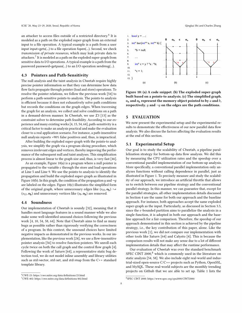
4.2 Taint AnalysisTo demonstrate that our approach is applicable to a broad range
of data flow analysis, in addition to the null analysis discussed in
the paper, we also implement a taint analysis to check two kinds
of taint issues. First, we check relative path traversal, which allows
Figure 10: (a) A code snippet. (b) The exploded super-graphbuilt based on a points-to analysis. (c) The simplified graph.oa and ob represent the memory object pointed to by a and b,respectively. y and ¬y on the edges are the path conditions.
5 EVALUATIONWe now present the experimental setup and the experimental re-
sults to demonstrate the effectiveness of our new parallel data flow
analysis. We also discuss the factors affecting the evaluation results
at the end of this section.
5.1 Experimental SetupOur goal is to study the scalability of Cheetah, a pipeline paral-lelization strategy for bottom-up data flow analysis. We did this
by measuring the CPU utilization rates and the speedup over a
conventional parallel implementation of our bottom-up analysis.
More specifically, a conventional parallel implementation only an-
alyzes functions without calling dependence in parallel, just as
illustrated in Figure 1. To precisely measure and study the scalabil-
ity of our approach, we introduce an artificial throttle that allows
us to switch between our pipeline strategy and the conventional
parallel strategy. In this manner, we can guarantee that, except for
the parallel strategies, all other implementation details discussed
in Section 4 are the same for both our approach and the baseline
approach. For instance, both approaches accept the same exploded
super-graph as the input. Particularly, as discussed in Section 3.5,
since the ϵ-bounded partition aims to parallelize the analysis in a
single function, it is adopted in both our approach and the base-
line approach for a fair comparison. Therefore, the speedup of our
approach demonstrated in this section is achieved by the pipeline
strategy, i.e., the key contribution of this paper, alone. Like the
previous work [1], we did not compare our implementation with
other tools like Saturn [64] and Calysto [4]. This is because the
comparison results will not make any sense due to a lot of different
implementation details that may affect the runtime performance.
Our evaluation of Cheetah was over the standard benchmark
SPEC CINT 2000,8which is commonly used in the literature on
static analysis [54, 58]. We also include eight real-world and indus-
trial-sized open-source C/C++ projects such as Python, OpenSSL,
and MySQL. These real-world subjects are the monthly trending
projects on Github that we are able to set up. Table 1 lists the
Figure 12: CPU utilization rate vs. The elapsed time. The solid lines represent the CPU utilization rate of our pipeline methodwhile the dashed lines represent that of the conventional parallel design.
5.3 Study of the Taint AnalysisIn order to demonstrate that our approach is generalizable to other
analyses, we also conducted an experiment to see whether the
pipeline approach can improve the scalability of taint analysis.
Since the result of taint analysis are quite similar to that of the null
analysis, we briefly summarize the experimental results in Table 3,
where the results of our largest benchmark program, MySQL, are
presented. The results demonstrate that, with the increase of the
number of available threads, the speedup of our approach over
the conventional approach also grows to >2× in analyzing both
the relative path traversal (RPT) bug or the transmission of privateresources (TPR) bug.
5.4 DiscussionThere are two main factors affecting the evaluation results: the
density of the call graph and the number of available threads.
As discussed above, when the call graph is very sparse, the
advantage of our approach is not very obvious. For instance, if
10
Pipelining Bottom-up Data Flow Analysis ICSE ’20, May 23–29, 2020, Seoul, Republic of Korea
RPT Time Out 10.2hr - Time Out 8.7hr - Time Out 7.1hr - 10.9hr 4.7hr 2.3×TPR 9.3hr 6.6hr 1.4× 8.1hr 5.0hr 1.6× 7.4hr 3.9hr 1.9× 6.1hr 2.8hr 2.2×
functions are all independent on each other, all functions can be run
in parallel. Thus, both approaches can always sufficiently utilize the
available threads and, thus, have similar time efficiency. In practice,
as demonstrated in our evaluation, the call graph is usually tree-like.
Thus, our approach can present its power in the second half of the
analysis and achieves up to 3× speedup in practice.
The number of threads is also a key factor affecting the ob-
served speedup of our approach. For instance, if we only have one
thread available, although our approach can provide more indepen-
dent tasks, these tasks cannot be run in parallel. Thus, both of our
approach and the conventional one will emit similar results. As
illustrated by the evaluation, our approach can work better when
we have more available threads. In the cloud era, we can expect
that we have unlimited CPU resources and, thus, can expect more
benefits from our approach in practice.
6 RELATEDWORKParallel and distributed algorithms for data flow analysis is an
active area of research. In this section, we survey existing parallel
or distributed techniques and compare them with Cheetah.In order to utilize the modular structure of a program to paral-
lelize the analyses in different functions, developers usually imple-
ment a data flow analysis in a top-down fashion or a bottom-up
manner. Albarghouthi et al. [1] presented a generic framework to
distribute top-down algorithms using a map-reduce strategy. Par-
allel worklist approaches, a kind of top-down analysis, also can
address the IFDS/IDE problems. They operate by processing the
elements on an analysis worklist in parallel [14, 21, 48]. These ap-
proaches are different from ours because this paper focuses on
bottom-up analysis. In our opinion, the top-down approach and the
bottom-up approach are two separate schools of methodologies to
implement program analysis. Bottom-up approaches analyze each
function only once and generate summaries reusable at all calling
contexts. Top-down approaches generate summaries that are spe-
cific to individual calling contexts and, thus, may need to repeat
analyzing a function. For analyses that need high precision like
path-sensitivity, repetitively analyzing a function is costly. Thus,
we may expect better performance from bottom-up analysis when
high precision is required.
Compared to top-down analysis, bottom-up analysis has been
traditionally easier to parallelize. Existing static analyses, such as
Saturn [64], Calysto [4], Pinpoint [54], and Infer [8], have utilizedthe function-level parallelization to improve their scalability. How-
ever, none of them presented any techniques to further improve its
parallelism. McPeak et al. [35] pointed out that the CPU utilization
rate may drop in the dense part of the call graph where the paral-
lelism is significantly limited by the calling dependence. Although
they presented an optimized scheduling method to mitigate the
performance issue, the calling dependence was not relaxed and
the function-level parallelism was not improved. We believe that
their scheduling method is complementary to Cheetah and their
combination has the potential for the greater scalability.
In contrast to top-down and bottom-up approaches, partition-
based approaches [6, 12, 17, 22, 26, 29, 33, 38] do not utilize the
modular structure of a program but partition the state space and
distribute the state-space search to several threads or processors.
Another category of data flow analyses (e.g., [2, 7, 25]) are modeled
as Datalog queries rather than the graph reachability queries in
the IFDS/IDE framework. They can benefit from parallel Datalog
engines to improve the scalability [20, 27, 28, 34, 51–53, 61, 62, 66].
Recently, some other parallel techniques have been proposed.
Many of them focus on pointer analysis [18, 31, 37, 41, 44, 57]
rather than general data flow analysis. Mendez-Lojo et al. [36]
proposed a GPU-based implementation for inclusion-based pointer
analysis. EigenCFA [43] is a GPU-based flow analysis for higher-
order programs. Graspan [60] and Grapple [68] turn sophisticated
code analysis into big data analytics. They utilize recent advances
on solid-state disks to parallelize and scale program analysis. These
techniques are not designed for compositional data flow analysis
and, thus, are different from our approach.
In addition to automatic techniques, Ball et al. [5] used manually
created harnesses to specify independent device driver entry points
so that an embarrassingly parallel workload can be created.
7 CONCLUSIONWe have presented Cheetah, a pipeline parallelization strategy
that enables to perform bottom-up data flow analysis in a faster
way. The pipeline strategy relaxes the calling dependence, which
conventionally limits the parallelism of bottom-up analysis. The
evaluation of our approach demonstrates higher CPU utilization
rates and significant speedup over a conventional parallel design.
In the multi-core era, we believe that improving the parallelism is
an important approach to scaling static program analysis.
ACKNOWLEDGMENTSThe authors would like to thank the anonymous reviewers for
their insightful comments. This work is partially funded by an
MSRA grant, as well as Hong Kong GRF16230716, GRF16206517,
ITS/215/16FP, and ITS/440/18FP grants.
REFERENCES[1] Aws Albarghouthi, Rahul Kumar, Aditya V Nori, and Sriram K Rajamani. 2012.
Parallelizing top-down interprocedural analyses. In Proceedings of the 33rd ACMSIGPLAN Conference on Programming Language Design and Implementation (PLDI’12). ACM, 217–228.
[2] Nicholas Allen, Padmanabhan Krishnan, and Bernhard Scholz. 2015. Combining
type-analysis with points-to analysis for analyzing Java library source-code. In
11
ICSE ’20, May 23–29, 2020, Seoul, Republic of Korea Qingkai Shi and Charles Zhang
Proceedings of the 4th ACM SIGPLAN International Workshop on State Of the Artin Program Analysis (SOAP ’15). ACM, 13–18.
[3] Steven Arzt, Siegfried Rasthofer, Christian Fritz, Eric Bodden, Alexandre Bar-
tel, Jacques Klein, Yves Le Traon, Damien Octeau, and Patrick McDaniel. 2014.
Flowdroid: Precise context, flow, field, object-sensitive and lifecycle-aware taint
analysis for android apps. In Proceedings of the 35th ACM SIGPLAN Conference onProgramming Language Design and Implementation (PLDI ’14). ACM, 259–269.
[4] Domagoj Babic and Alan J. Hu. 2008. Calysto: Scalable and precise extended
static checking. In Proceedings of the 30th International Conference on SoftwareEngineering (ICSE ’08). IEEE, 211–220.
[5] Thomas Ball, Vladimir Levin, and Sriram K Rajamani. 2011. A decade of software
model checking with SLAM. Commun. ACM 54, 7 (2011), 68–76.
in SPIN. In International SPIN Workshop on Model Checking of Software. Springer,200–216.
[7] Martin Bravenboer and Yannis Smaragdakis. 2009. Strictly declarative specifica-
tion of sophisticated points-to analyses. In Proceedings of the 24th ACM SIGPLANConference on Object Oriented Programming Systems Languages and Applications(OOPSLA ’09). ACM, 243–262.
[8] Cristiano Calcagno, Dino Distefano, Peter W. O’Hearn, and Hongseok Yang. 2011.
Compositional shape analysis by means of bi-abduction. J. ACM 58, 6 (2011),
26:1–26:66.
[9] Sagar Chaki, Edmund M Clarke, Alex Groce, Somesh Jha, and Helmut Veith. 2004.
Modular verification of software components in C. IEEE Transactions on SoftwareEngineering 30, 6 (2004), 388–402.
[10] Sigmund Cherem, Lonnie Princehouse, and Radu Rugina. 2007. Practical memory
leak detection using guarded value-flow analysis. In Proceedings of the 28th ACMSIGPLAN Conference on Programming Language Design and Implementation (PLDI’07). ACM, 480–491.
[11] Chia Yuan Cho, Vijay D’Silva, and Dawn Song. 2013. BLITZ: Compositional
bounded model checking for real-world programs. In Proceedings of the 28thIEEE/ACM International Conference on Automated Software Engineering (ASE ’13).IEEE, 136–146.
[12] Liviu Ciortea, Cristian Zamfir, Stefan Bucur, Vitaly Chipounov, and George
[13] Leonardo De Moura and Nikolaj Bjørner. 2008. Z3: An efficient SMT solver. In
International conference on Tools and Algorithms for the Construction and Analysisof Systems. Springer, 337–340.
[14] Kyle Dewey, Vineeth Kashyap, and Ben Hardekopf. 2015. A parallel abstract
interpreter for JavaScript. In 2015 IEEE/ACM International Symposium on CodeGeneration and Optimization (CGO ’15). IEEE, 34–45.
[15] Isil Dillig, Thomas Dillig, and Alex Aiken. 2008. Sound, complete and scalable
path-sensitive analysis. In Proceedings of the 29th ACM SIGPLAN Conference onProgramming Language Design and Implementation (PLDI ’08). ACM, 270–280.
[16] Isil Dillig, Thomas Dillig, Alex Aiken, andMooly Sagiv. 2011. Precise and compact
modular procedure summaries for heap manipulating programs. In Proceedingsof the 32nd ACM SIGPLAN Conference on Programming Language Design andImplementation (PLDI ’11). ACM, 567–577.
[17] Matthew B Dwyer, Sebastian Elbaum, Suzette Person, and Rahul Purandare. 2007.
Parallel randomized state-space search. In Proceedings of the 29th InternationalConference on Software Engineering (ICSE ’07). IEEE, 3–12.
[18] Marcus Edvinsson, Jonas Lundberg, and Welf Löwe. 2011. Parallel points-to
analysis for multi-core machines. In Proceedings of the 6th International Conferenceon High Performance and Embedded Architectures and Compilers. ACM, 45–54.
[19] Stephen J Fink, Eran Yahav, Nurit Dor, G Ramalingam, and Emmanuel Geay. 2008.
Effective typestate verification in the presence of aliasing. ACM Transactions onSoftware Engineering and Methodology (TOSEM) 17, 2 (2008), 9.
[20] Sumit Ganguly, Avi Silberschatz, and Shalom Tsur. 1990. A Framework for the
Parallel Processing of Datalog Queries. In Proceedings of the 1990 ACM SIGMODInternational Conference on Management of Data (SIGMOD ’90). ACM, 143–152.
[21] Diego Garbervetsky, Edgardo Zoppi, and Benjamin Livshits. 2017. Toward full
elasticity in distributed static analysis: the case of callgraph analysis. In Proceed-ings of the 2017 11th Joint Meeting on Foundations of Software Engineering (FSE’17). ACM, 442–453.
Bernhard Scholz, and Yi Lu. 2017. An efficient tunable selective points-to anal-
ysis for large codebases. In Proceedings of the 6th ACM SIGPLAN International
Workshop on State Of the Art in Program Analysis (SOAP ’17). ACM, 13–18.
[26] Gerard J Holzmann and Dragan Bosnacki. 2007. The design of a multicore
extension of the SPIN model checker. IEEE Transactions on Software Engineering33, 10 (2007), 659–674.
[27] G. Hulin. 1989. Parallel Processing of Recursive Queries in Distributed Archi-
tectures. In Proceedings of the 15th International Conference on Very Large DataBases (VLDB ’89). Morgan Kaufmann Publishers Inc., 87–96.
[28] Herbert Jordan, Pavle Subotić, David Zhao, and Bernhard Scholz. 2019. A spe-
cialized B-tree for concurrent datalog evaluation. In Proceedings of the 24th Sym-posium on Principles and Practice of Parallel Programming (PPoPP ’19). ACM,
327–339.
[29] Yong-fong Lee and Barbara G Ryder. 1992. A comprehensive approach to par-
allel data flow analysis. In Proceedings of the 6th International Conference onSupercomputing. ACM, 236–247.
[30] Jan Karel Lenstra and AHG Rinnooy Kan. 1978. Complexity of scheduling under
precedence constraints. Operations Research 26, 1 (1978), 22–35.
[31] Bozhen Liu, Jeff Huang, and Lawrence Rauchwerger. 2019. Rethinking Incremen-
tal and Parallel Pointer Analysis. ACM Transactions on Programming Languagesand Systems (TOPLAS) 41, 1 (2019), 6.
[32] Benjamin Livshits, Manu Sridharan, Yannis Smaragdakis, Ondřej Lhoták, J Nelson
Amaral, Bor-Yuh Evan Chang, Samuel Z Guyer, Uday P Khedker, Anders Møller,
and Dimitrios Vardoulakis. 2015. In defense of soundiness: a manifesto. Commun.ACM 58, 2 (2015), 44–46.
[33] Nuno P Lopes and Andrey Rybalchenko. 2011. Distributed and predictable soft-
ware model checking. In International Workshop on Verification, Model Checking,and Abstract Interpretation. Springer, 340–355.
[34] Carlos Alberto Martínez-Angeles, Inês Dutra, Vítor Santos Costa, and Jorge
Buenabad-Chávez. 2013. A datalog engine for gpus. In Declarative Programmingand Knowledge Management. Springer, 152–168.
[35] Scott McPeak, Charles-Henri Gros, and Murali Krishna Ramanathan. 2013. Scal-
able and incremental software bug detection. In Proceedings of the 2013 9th JointMeeting on Foundations of Software Engineering (ESEC/FSE ’13). ACM, 554–564.
[36] Mario Mendez-Lojo, Martin Burtscher, and Keshav Pingali. 2012. A GPU imple-
mentation of inclusion-based points-to analysis. In Proceedings of the 17th ACMSIGPLAN Symposium on Principles and Practice of Parallel Programming (PPoPP’12). ACM, 107–116.
[37] Mario Méndez-Lojo, Augustine Mathew, and Keshav Pingali. 2010. Parallel
inclusion-based points-to analysis. In Proceedings of the ACM International Con-ference on Object Oriented Programming Systems Languages and Applications(OOPSLA ’10). ACM, 428–443.
[38] David Monniaux. 2005. The parallel implementation of the Astrée static analyzer.
In Asian Symposium on Programming Languages and Systems. Springer, 86–96.[39] Nomair A Naeem and Ondrej Lhotak. 2008. Typestate-like analysis of multiple
interacting objects. In Proceedings of the 23rd ACM SIGPLAN Conference on Object-oriented Programming Systems Languages and Applications (OOPSLA ’08). ACM,
347–366.
[40] Nomair A Naeem and Ondrej Lhoták. 2009. Efficient alias set analysis using SSA
form. In Proceedings of the 2009 International Symposium on Memory Management(ISMM ’09). ACM, 79–88.
[41] Vaivaswatha Nagaraj and R Govindarajan. 2013. Parallel flow-sensitive pointer
analysis by graph-rewriting. In Proceedings of the 22nd International Conferenceon Parallel Architectures and Compilation Techniques. IEEE, 19–28.
[42] Damien Octeau, Patrick McDaniel, Somesh Jha, Alexandre Bartel, Eric Bodden,
Jacques Klein, and Yves Le Traon. 2013. Effective inter-component communica-
tion mapping in android: An essential step towards holistic security analysis. In
Presented as part of the 22nd USENIX Security Symposium (USENIX Security ’13).USENIX Association, 543–558.
[43] Tarun Prabhu, Shreyas Ramalingam, Matthew Might, and Mary Hall. 2011.
EigenCFA: Accelerating flow analysis with GPUs. In Proceedings of the 38thAnnual ACM SIGPLAN-SIGACT Symposium on Principles of Programming Lan-guages (POPL ’11). ACM, 511–522.
[44] Sandeep Putta and Rupesh Nasre. 2012. Parallel replication-based points-to
analysis. In International Conference on Compiler Construction (CC ’12). Springer,61–80.
[45] Thomas Reps, Susan Horwitz, and Mooly Sagiv. 1995. Precise interprocedural
dataflow analysis via graph reachability. In Proceedings of the 22nd ACM SIGPLAN-SIGACT Symposium on Principles of Programming Languages (POPL ’95). ACM,
49–61.
[46] Thomas Reps, Susan Horwitz, Mooly Sagiv, and Genevieve Rosay. 1994. Speeding
up slicing. In Proceedings of the 2nd ACM SIGSOFT Symposium on Foundations ofSoftware Engineering (FSE ’94). ACM, 11–20.
[47] Noam Rinetzky, Mooly Sagiv, and Eran Yahav. 2005. Interprocedural shape
analysis for cutpoint-free programs. In International Static Analysis Symposium.
Springer, 284–302.
[48] Jonathan Rodriguez and Ondřej Lhoták. 2011. Actor-based parallel dataflow
analysis. In International Conference on Compiler Construction (CC ’11). Springer,179–197.
12
Pipelining Bottom-up Data Flow Analysis ICSE ’20, May 23–29, 2020, Seoul, Republic of Korea
[49] Atanas Rountev, Mariana Sharp, and Guoqing Xu. 2008. IDE dataflow analysis
in the presence of large object-oriented libraries. In International Conference onCompiler Construction (CC ’08). Springer, 53–68.
[50] Mooly Sagiv, Thomas Reps, and Susan Horwitz. 1996. Precise interprocedural
dataflow analysis with applications to constant propagation. Theoretical ComputerScience 167, 1 (1996), 131–170.
[51] Bernhard Scholz, Herbert Jordan, Pavle Subotić, and Till Westmann. 2016. On fast
large-scale program analysis in datalog. In International Conference on CompilerConstruction (CC ’16). ACM, 196–206.
[52] Jürgen Seib and Georg Lausen. 1991. Parallelizing Datalog programs by gen-
eralized pivoting. In Proceedings of the tenth ACM SIGACT-SIGMOD-SIGARTsymposium on Principles of database systems. ACM, 241–251.
[53] Marianne Shaw, Paraschos Koutris, Bill Howe, and Dan Suciu. 2012. Optimizing
large-scale Semi-Naïve datalog evaluation in hadoop. In International Datalog 2.0Workshop. Springer, 165–176.
[54] Qingkai Shi, Xiao Xiao, Rongxin Wu, Jinguo Zhou, Gang Fan, and Charles Zhang.
2018. Pinpoint: Fast and precise sparse value flow analysis for million lines
of code. In Proceedings of the 39th ACM SIGPLAN Conference on ProgrammingLanguage Design and Implementation (PLDI ’18). ACM, 693–706.
[55] Sharon Shoham, Eran Yahav, Stephen J Fink, and Marco Pistoia. 2008. Static
[56] Bjarne Steensgaard. 1996. Points-to analysis in almost linear time. In Proceedingsof the 23rd ACM SIGPLAN-SIGACT symposium on Principles of programminglanguages. ACM, 32–41.
[57] Yu Su, Ding Ye, and Jingling Xue. 2014. Parallel pointer analysis with CFL-
reachability. In 2014 43rd International Conference on Parallel Processing. IEEE,451–460.
[58] Yulei Sui, Ding Ye, and Jingling Xue. 2014. Detecting memory leaks statically
with full-sparse value-flow analysis. IEEE Transactions on Software Engineering40, 2 (2014), 107–122.
[59] Omer Tripp, Marco Pistoia, Patrick Cousot, Radhia Cousot, and Salvatore
Guarnieri. 2013. Andromeda: Accurate and scalable security analysis of web
applications. In International Conference on Fundamental Approaches to Software
Engineering. Springer, 210–225.[60] Kai Wang, Aftab Hussain, Zhiqiang Zuo, Guoqing Xu, and Ardalan Amiri Sani.
2017. Graspan: A single-machine disk-based graph system for interprocedural
static analyses of large-scale systems code. ACM SIGOPS Operating SystemsReview 51, 2 (2017), 389–404.
[61] Ouri Wolfson and Aya Ozeri. 1990. A New Paradigm for Parallel and Distributed
Rule-processing. In Proceedings of the 1990 ACM SIGMOD International Conferenceon Management of Data (SIGMOD ’90). ACM, 133–142.
[62] Ouri Wolfson and Avi Silberschatz. 1988. Distributed Processing of Logic Pro-
grams. In Proceedings of the 1988 ACM SIGMOD International Conference onManagement of Data (SIGMOD ’88). ACM, 329–336.
[63] Yichen Xie and Alex Aiken. 2005. Context- and path-sensitive memory leak
detection. In Proceedings of the 10th European Software Engineering ConferenceHeld Jointly with 13th ACM SIGSOFT International Symposium on Foundations ofSoftware Engineering (ESEC/FSE ’05). ACM, 115–125.
[64] Yichen Xie and Alex Aiken. 2005. Scalable error detection using Boolean satisfia-
bility. In Proceedings of the 32nd ACM SIGPLAN-SIGACT Symposium on Principlesof Programming Languages (Long Beach, California, USA) (POPL ’05). ACM,
Distefano, and Peter O’Hearn. 2008. Scalable shape analysis for systems code. In
International Conference on Computer Aided Verification. Springer, 385–398.[66] Mohan Yang, Alexander Shkapsky, and Carlo Zaniolo. 2017. Scaling up the
performance of more powerful Datalog systems on multicore machines. TheVLDB Journal - The International Journal on Very Large Data Bases 26, 2 (2017),229–248.
[67] Greta Yorsh, Eran Yahav, and Satish Chandra. 2008. Generating precise and
concise procedure summaries. In Proceedings of the 35th Annual ACM SIGPLAN-SIGACT Symposium on Principles of Programming Languages (POPL ’08). ACM,
221–234.
[68] Zhiqiang Zuo, John Thorpe, Yifei Wang, Qiuhong Pan, Shenming Lu, Kai Wang,
Guoqing Harry Xu, Linzhang Wang, and Xuandong Li. 2019. Grapple: A graph
system for static finite-state property checking of large-scale systems code. In
Proceedings of the Fourteenth EuroSys Conference 2019 (EuroSys ’19). ACM, 38.