1

PIV Investigation of the Flow Characteristics in an Internal CoolantPassage with Two Ducts Connected by a Sharp 180º Bend

J. Schabacker, A. BölcsSwiss Federal Institute of Technology

EPFL-LTTLausanne, Switzerland

B.V. JohnsonABB Corporate Research

Baden, Switzerland

Abstract

A PIV study of the flow in a stationary model of a smooth two-passinternal coolant passage is presented, which focuses on the flowcharacteristics in the sharp 180º bend and downstream of the bendwhere the flow is redeveloping. Because PIV in its traditionalconception only allows for the investigation of two-dimensional flow,a stereoscopic digital PIV system was assembled that measures allthree velocity components simultaneously. The mean-velocity fieldand turbulence quantities of the flow are obtained from the PIVmeasurements.The model of the coolant passage consists of two square ducts, eachhaving a length of 19 hydraulic diameters, which are connected by asharp 180º bend with a rectangular outer wall. The measurementswere obtained at one flow condition with a flow Reynolds number of50,000. A strong secondary flow motion occurs in the bend of thesmooth passage that consists of two counter rotating vortices, whichimpinge on the outer wall and influence the flow in the downstreamleg. Both of the outer corners contain regions of recirculating flow. Aseparation bubble, about 1.5 hydraulic diameters long, occurs on theinner wall of the return pass. In the symmetry plane, the flow recoversfrom the bend effect within 10 hydraulic diameters.

Nomenclature

x Cartesian coordinate in axial duct directiony Cartesian coordinate in cross duct directionz Cartesian coordinate in horizontal duct directionΦ Cylindrical coordinate in streamwise directionr Cylindrical coordinate in radial directionU Mean velocity component in x directionV Mean velocity component in y directionW Mean velocity component in z directionUφ Mean velocity component in streamwise direction in bendUr Mean velocity component in radial direction in bendu’ Fluctuating velocity component in axial directionv’ Fluctuating velocity component in cross duct direction

w’ Fluctuating velocity component in vertical directionu’φ Fluctuating velocity component in streamwise directionu’r Fluctuating velocity component in radial directionu’v’,u’w’ Cartesian components of turbulent shear stressUb Bulk mean-velocityD Height and width of passage legs, D=100 mmDh Hydraulic diameter Dh =DB Thickness of divider plateS Section length in bend at 90° section, S/Dh=1.05α Section angle in bendk Turbulent kinetic energy

( )( ) ( )( )bendin

U

'wuu2

1

U

'w'v'u2

1

2b

22'r

2'

2b

222 ++⇔

++ Φ

proj Projected distance in bend =

( )

( )°≤α<°

α+

°>α°≤αα+

13545forS

sinzx

135and45forS

coszx

22

22

Introduction

Advanced gas turbines are designed to operate with high efficiency todecrease fuel consumption as well as the pollution of the environment.From basic thermodynamic consideration, it can be derived that theefficiency of the gas turbine process cycle rises with higher turbinepressure ratios and more importantly with higher turbine inlettemperatures.The maximum turbine inlet temperature, however, is limited by theavailability of blade material that can withstand such hightemperatures and stresses. During the last 50 years a considerableincrease of the turbine inlet temperature has been achieved, e.g. inLakshminarayana (1996). Modern materials can withstandtemperatures of about 1200K. Present gas turbines operate at turbineinlet temperatures of approximately 1550K. Effective cooling isapplied to the turbine components that are exposed to the hot stream.

2

For this, a combination of internal and external cooling methods istypically employed to lower the mean blade temperature to allowablevalues.

Internal cooling of turbine blades

For the internal cooling of the blades, the coolant is passed through amultipass circuit from hub to tip and ejected at the trailing edge or theblade tip. The straight sections of these coolant passages areconnected by 180º bends. To enhance heat transfer, the walls areroughened by ribs or pin fins that lead to very complicated flowpatterns in the passage.In the sharp 180º bends, a Dean-type secondary motion is established.The secondary flow is formed by the imbalance between the radialpressure gradient and the centrifugal force that acts on the fluid. Dueto the streamline curvature, a radial pressure gradient develops acrossthe bend section with a higher pressure near the outer radius surface.The pressure imbalance acts on the slowly moving fluid near thesidewalls of the bend and displaces it along the sidewalls from theouter to the inner radius wall. Near the symmetry plane, the turning ofthe high momentum fluid produces centrifugal forces that drive theflow radially outward towards the outer radius wall. Consequently, asecondary flow field with two counter-rotating vortices develops inthe bends of stationary passages.The effect of the bend on the heat transfer in smooth and ribbedstationary passages has been experimentally studied by Johnson andLaunder. (1985), Metzger and Sahm (1986), Han et al. (1988), Hanand Zhang (1991), and Ekkad and Han (1995). The secondary flowsand flow separation at the tip of the divider plate influence the heattransfer in the bend. As the flow progresses through the bend of asmooth passage, the presence of the secondary flow causes higherheat transfer on the top and bottom wall as well as on the outer wall.This was attributed to the higher turbulence of the flow andimpingement in conjunction with the transport of cold fluid from thebulk towards the walls. Downstream of the bend, high turbulencemixing by flow separation and reattachment on the divider plate leadsto an additional increase of the heat transfer. In passages, whereoblique ribs are mounted in the straight sections, the ribs create asecondary flow, which interacts with the curvature induced secondaryflow in the bend. This leads to very complicated flow fields in theturning region.For the design of gas turbine blades, a detailed knowledge of thephysical phenomena in the passage is necessary. Although CFDsimulations can provide a better understanding of these phenomena,the numerical heat transfer predictions are not yet sufficiently accuratefor design purposes. This is especially true for the complicated heattransfer patterns in the turning region of stationary or rotating coolantpassages with rib roughened walls. To improve the performance of theCFD codes, a validation of the predictions is necessary and detailedmeasurements of the flow structure in the passages are required forcomparison.Previous experiments to define the flow characteristics and to providedata for CFD evaluation have included LDV measurements in rotatingand stationary two-pass passages by Cheah et al. (1994) and Iacovideset al. (1996). Liou and Chen (1997) recently performed LDVmeasurements of the developing flow through a smooth duct with a180º straight-corner turn. Tse and Steuber (1997) reported 3D LDVmeasurements in rotating square serpentine coolant passage withskewed ribs.

PIV technique

In the present study, the particle-image-velocimetry (PIV) methodwas employed for the investigation of the flow field in a model of astationary two-pass coolant passage. PIV was chosen for such a studybecause of its high data acquisition rate and the good spatial

resolution of the measured flow fields. These features are obtainedbecause PIV performs full-flow field measurements in a sheet of lightin the flow. A good selection of papers on PIV can be found in Grant(1994). The reader is referred to this reference for a more detaileddiscussion of the requirements for the setup of PIV experiments.Few PIV studies of flows in turbomachinery have been reported todate. Bryanston-Cross et al. (1991) carried out experiments in atransonic turbine cascade. Tisserant and Breugelsmans (1995)performed rotor blade-to-blade velocity measurements and Gogineniet al. (1996) studied periodically forced flat plate film cooling.The measurements of highly three-dimensional flow with a single-camera PIV system could have substantial errors because the out-of-plane motion of a particles perpendicular to the light sheet planeproduces a systematic measurement error that increases withincreasing distance from the optical axis, e.g., Lourenco (1988). Inprinciple, an error correction for the in-plane components is feasible ifthe out-of-plane component of the flow is known. Schabacker andBölcs (1996) applied the correction to single-camera 3D PIV velocitymeasurements and showed that the effect of the out-of-plane motioncan not be corrected completely, although the correction improves themeasurement accuracy.This measurement error can be avoided with a stereoscopic PIV setup.A comprehensive analysis of the translation method, photographicrecording, PIV-like evaluation of the separate records, matching of thedata for three-dimensional velocity vectors and an application torotating disc flow has been given by Prasad and Adrian (1993).Westerweel and Nieuwstadt (1991) have reported performance testson three-dimensional velocity measurements with a digital two-camera stereoscopic PIV system.There are two possible stereoscopic PIV configurations with which toview the light sheet at an oblique angle. In the angular displacementmethod, the imaging systems point at the particle field such that theiroptical axis form the required stereo angles with the light sheet.However, the oblique orientation of the object plane results in a tiltedplane so that a normal camera could have focusing problems.Therefore, the angle is often kept so small that the resultingdefocusing is acceptable. In the translation method, the imagingsystems are aligned to right angles to the light sheet. The commonfield of view is limited due to the axial distance required for sufficientaccuracy. Nevertheless, translating the back planes of the cameras canincrease the common field of view (Hinsch 1995).For the present investigation, a stereoscopic digital PIV system thatemploys the angular displacement method and commercially availabledevices was assembled. No modifications to the cameras were made.The small amount of defocusing of the images towards the edges wasfound to have a minor influence and was tolerated. The system iscapable of measuring simultaneously all three velocity components.Subsequently, an ensemble average of the velocity data in identicalspatial windows is calculated leading to the mean and fluctuatingvelocity field.

Objectives of the study

The objectives of the present paper are:

• To demonstrate that the stereoscopic PIV technique is capable ofobtaining detailed statistical data that can be used for theevaluation of turbulence models in complex three-dimensionalflows.

• To obtain and present data for turbulent flow in a smooth internalcoolant passage with a sharp 180º bend as the first demonstrationcase.

3

Experimental Setup

Test Facility

A sketch of the test section is shown in Figure 1. Air was chosen asthe working medium because heat transfer experiments will beconducted in the same facility in the near future. A continuouslyrunning compressor supplies the air to the test rig. Upstream of thetest-rig, the mass flow rate is measured by means of an orifice meter.The air enters the settling chamber with an inner diameter of 600 mmvia a 150 mm tube and a conical entrance section with an angle of30°. The settling chamber is equipped with a combination ofperforated plates, honeycombs and meshes to reduce unsteadiness andswirl in the flow. For the PIV experiments, 1-3 µm oil dropletsgenerated by a Polytec L2F-A-1000 Aerosol Generator are injectedupstream of the settling chamber to guarantee a homogeneous seedingdensity in the test section.

20 Dh

1D

h2.1 Dh

Outflow

Square Cross Section: 1x1 Dh

Inner Wall

1.05 Dh

0.1 Dh 90deg corner

Figure 1 The internal coolant passage test facility

A modular concept was chosen for the test section design that allowsan easy exchange of the components. Presently, the test rig isequipped with a model of a two-pass cooling passage of a gas turbineblade. The flow path in the downstream and upstream leg has a cross-section of 100x100 mm2 with a corresponding hydraulic diameterDh=100 mm and a length of 19Dh. The test section is made of 5-mmthick float glass to obtain good optical properties for the PIVexperiment. In the straight-corner turn, the clearance between the tipof the divider plate and the outer wall is equal to 1.05Dh. Thethickness of the divider plate is 0.1Dh.The total section including the section entrance can be turned 90°around the x-axis without changing the flow conditions in the duct.This allows an easy optical access to the positions of interest for thePIV measurements.

Origin

y

x

z

zx

Φ r

α

Figure 2 Definition of coordinate system. Left side: Cartesian system.Right side: Cylindrical system in bend

The definition of the coordinate systems in the test facility is shown inFigure 2. Two coordinate systems are used, a cartesian and acylindrical. For both coordinate systems, the origin is set on thebottom wall at the turn entrance/exit plane. In the Cartesian (x,y,z)system, x is defined as positive in the streamwise direction of the flowdownstream of the bend exit, y is defined positive vertically upwardsin the horizontal test section orientation, and z is defined as shown.

In the cylindrical (Φ,r,y) coordinate system, the radial component r isdefined as positive in the direction towards the inner wall, thestreamwise component Φ is defined as positive following the flowalong the circular path centered on the center of the bend, and y isdefined as for the Cartesian system.

The PIV system

Cameras Lens

f = -50mm

Mirror

Light Sheet

Test Section

Laser

Traversing System

f = 300mmf = 76.2mm

Figure 3 PIV setup

A Quantel TwinsB Nd-Yag double oscillator pulsed laser provideslight pulses having a maximum energy of 320 mJ at a wavelength of532 nm. The time delay between a pair of pulses can be adjusted from1µs to 1s with a pulse duration of 5 ns. A plano-concave lens (-30 mmfocal length) combined with two plano-cylindrical lenses (76.2 and300 mm focal length) transform the beam into a thin vertical lightsheet. By adjusting the distance between these lenses, the desiredthickness and width of the light sheet can be obtained. All lenses havean anti-reflection coating. The complete system including laser, lightsheet optics and camera is mounted on a traversing system shown inFigure 3 that allows an easy traverse to the position of interest.

Kodak ES1.0Quantel Twins BNd-Yag laser

TTL signal

8 bit digital videooutput

ITI PCI frame grabberwith 2Mb memory on board

PC Pentium 15064 Mb Ram 8 GB hard disk space

2 Kodak ES1.0

Quantel Twins BNd-Yag laser

TTL signal

PC camera 1

PC camera 2

Figure 4 Digital PIV system

A sketch of the digital PIV system is shown in Figure 4. The systemconsists of two independent Kodak ES1.0 cameras each having itsown PC. The ES1.0 has a CCD interline transfer sensor, which has apixels array of 1008(H) by 1018(V) pixels. Each pixel measures ninemicrons square with a 60% fill factor using a microlens. The cameraoutputs 8 bit digital images with 256 gray levels. For PIVapplications, the camera is used in a special double exposure frametriggering mode. This mode allows the capture of two images

4

separated by a delay ranging from 2 µs to 66 ms. Nikkor 55mm microlenses are mounted on the cameras. For a typical recording situation,the cameras are placed with an oblique angle of 5º at a distance of0.7m from the light sheet plane.The PIV image acquisition starts with a signal from the laser. Twoimages are captured in rapid succession. This is accomplished bycapturing the first image in the photo diode array, transferring thisimage to the CCD array and then capturing a second image in thephoto diode array. The first image is transferred from the CCD to theframe grabber while the second image is being captured by the photodiode array. The second image is then transferred into the CCD arrayand subsequently onto the frame grabber’s second image buffer. Theframe grabber is an Imaging Technology PCI frame grabber with 2MB memory onboard. The PCs are equipped with 64 MB RAM and 8GB hard disk space. During the PIV measurement series, 50 imagesare written in real time into the PC’s RAM memory. Subsequently,the acquisition is stopped and the images are saved on the hard disk.

Data Reduction

The PIV recordings from the right and left camera are interrogatedindependently with the PIV software package VISIFLOW from AEATechnology. For the images, a cross-correlation analysis method isused with an interrogation window size of 64 by 64 pixels and 50%overlap between the interrogation windows. The Kodak cameraacquires images with a resolution of 1008 by 1018 pixels. Eachrecording results in a 30 by 30 vector field of the instantaneousvelocity. Usually the data contains a small number of spurious vectors(<2%). The vector field is therefore validated with predefinedthresholds for the vector continuity and velocity magnitude. Vectorsthat do not fall within the thresholds are removed and the remaininggaps are filled by a weighted average of surrounding vectors.From the processed vector fields, the instantaneous three-dimensionalvelocity field can be reconstructed. For angular PIV systems, whereboth cameras observe the light sheet from the same side, thecorresponding interrogation positions for the two images in the planeof the light sheet do not match in general. Therefore, a calibration ofthe camera system is performed that also corrects for the distortion ofthe images in the lenses and the glass walls of the passage.

Camera Left

Image 1L Image 2L

Camera Right

Image 1R Image 2R

Calibration Image

Figure 5 Calibration of the stereoscopic PIV system

A precision grid inserted into the field of view was used by others tofind the matching points into the two images. In the present study,however, this is troublesome, since it requires opening the test sectionfrequently. An alternative non-intrusive calibration technique wasdeveloped using the fact that both cameras record an identical particlepattern. For low particle densities, individual particles could beidentified in corresponding images from the right and left camera andbe used for the calibration of the camera arrangement. However, fortypical particle densities in PIV images, it is difficult to find identicalparticles in both images. Therefore, groups of particles are correlatedinstead of tracking individual particles. Thus, a displacement field isprocessed from two corresponding images as shown in Figure 5.

The displacement vectors are arranged on a regular grid that isidentical to the grid of the processed velocity vectors from the twocameras. In a subsequent step, the instantaneous three-dimensionalvelocity field can be reconstructed from the parallax (the apparentdifference in the recorded displacements between the right and leftimage) between the images. For this, the velocity fields from the rightand left camera are interpolated on an identical grid according to theallocation specification found from the calibration. For theinterpolation, a linear algorithm is fitted to the measurements.For more information on stereoscopic PIV imaging, the reader isreferred to Westerweel and Nieuwstadt (1991). Note that thestereoscopic measurements provide the third velocity component, buteven if the out-of-plane component is not required, stereoscopicrecording increases the measurement accuracy because it corrects thein-plane velocity for the effects of perspective.For most industrial applications, the engineers are interested not onlyin the instantaneous flow but also more importantly in the mean-velocity field and the turbulence quantities of the flow. In order toobtain PIV measurements in this form, the statistical distribution ofthe velocity components is calculated in identical spatial windows in aseries of instantaneous PIV measurements. From these statisticaldistributions, the ensemble average and the statistical central momentsare calculated which yield the desired mean-velocity field andReynolds stresses.

Applicability of the PIV technique to the presentedinvestigation

The previously presented PIV system provides velocity data at thelocation of the light sheet in the test section. All three velocitycomponents and their turbulence quantities are measuredsimultaneously. The date acquisition rate and spatial resolution of thefull-plane measurements is relatively high compared to conventional“point measurement” techniques as for example LDV. That is,because for a typical PIV experiment with the presented system, amatrix of 30x30 points is measured simultaneously with a point-wisedata acquisition rate of approximately 2000 samples/hour. From the soobtained detailed vector map of the flow field, a good understandingof the 3D steady flow phenomena can be obtained particularly whenthe measurement plane is scanned through the flow volume. The datais arranged on a regular grid and is therefore ideally suited for thecomparison with numerical flow simulations.One sample, being a pair of PIV recordings, requires about 2Mb ofdisk space and thus limits the possible sample size for the calculationof mean velocities and turbulence quantities causing relatively highmeasurement uncertainty. For the mean velocity components, themeasurement uncertainty can easily be decreased to lower levels ifone concentrates on a single measurement plane in the flow field andincreases the sample size there. However, for the PIV measurement ofnormal and shear stresses with an accuracy comparable to thatobtained from single-point measurement techniques far more sampleswould be required that currently cannot be acquired with state-of-the-art video and computer technique. Furthermore, the uncertainty in thestereoscopic measurements of the normal and shear stressesperpendicular to the light sheet plane is higher than that of the stresseswithin the light sheet plane due to the reconstruction of the velocityfield. For this reason in the present study only the in-plane Reynoldsstresses are presented. Another limitation of the PIV technique is thesize of the measurement volume in the flow that is determined by thesize of the interrogation window for the PIV image analysis. For thepresented measurements, each vector represents the average of theflow within a volume of approximately 6x6x1mm3, which is ratherlarge. In principle, the size of the measurement volume could bedecreased by increasing the magnification of the PIV recordings. Forthe angular stereoscopic system, the reduced depth of field of the PIV

5

recording imposes a lower limit for the measurement volume as thedistance between measurement-plane and image-plane of the camerasdecreases. This effect is due to unfocused particles in the recordingsthat effect the measurement accuracy.In the present study, therefore the measurements focus on the large-scale turbulent interaction, which drive the overall flow field. Theflow was investigated in various planes within the bend anddownstream of the bend providing a good understanding of the largescale flow phenomena and with some restrictions also for the smallscale phenomena in the bend corners shown in Figure 8, where theimage magnification was increased. The authors believe that despitethe limitation of PIV in terms of measurement accuracy andmeasurement volume, the results can be used for the validation ofnumerical codes. For the near wall characteristics of the flow it isrecommended to combine the PIV technique with single-pointmeasuring techniques.

Measurements program and flow condition

Detailed measurements of the flow structure in a smooth two-passpassage have been obtained upstream and downstream of the sharp180º bend and in the bend. The flow Reynolds number was 50,000.As mentioned previously, the PIV system is mounted on a traversingunit that allows a flexible positioning of the light sheet plane in theposition of interest. Typically, the PIV experiments were carried outin such a way that, at a constant streamwise position, measurementswere taken in nine parallel planes, 0.1Dh apart. The test section wasthen turned and the measurements were repeated yielding a grid ofmeasurement planes in Figure 6 from which the three-dimensionalvelocity field can be obtained.

Vertical measurement planes

Horizontal measurement planes

Figure 6 Combination of measurement planes

The vector maps that are presented in Figure 13 and Figure 15 wereobtained from such a combination of measurement grids and thushave a more qualitative character. All other vector maps and profileswere extracted directly from the measurement planes and falltherefore within the uncertainty range specified in the followingsection.

Uncertainty

The estimation of the uncertainty of stereoscopic PIV velocitymeasurements requires the consideration of several aspects.Systematic errors occur due to the uncertainty in the determination ofthe geometrical parameter and the fabrication tolerances of the cameradevices and lenses. Non-systematic errors are mainly due to theuncertainty in the determination of the average particle displacementin the interrogation region. The errors depend on the size of the

interrogation region, the time separation between the laser pulses, themagnification of the recording, the out-of-plane velocity component,the turbulence of the flow, the length scale of the flow etc. The choiceof the recording and interrogation parameters is therefore ofsignificant importance for accurate and reliable velocitymeasurements.To quantify the measurement uncertainty of the stereoscopic PIVsystem, an experimental study has been conducted. Typically, 100 –400 samples were ensemble averaged on each measurement plane.From these measurements, it was determined that for the presentedstudy the 95% confidence interval for the mean-velocity field is lessthan 0.02Ub in regions where the flow behaves well. Such a region is,for instance, the quasi two-dimensional flow in the bend symmetryplane as shown Figure 10. To quantify the uncertainty, the figure alsoincludes the uncertainty interval for the mean velocities in Figure10a+b. However, in regions of high turbulence and three-dimensionalflow, as for example downstream of the bend exit in Figure 16a, the95% confidence interval for the mean velocities increases to 0.10Ub.Due to the small sample size, the uncertainty interval for thecorresponding turbulence quantities is rather high. The 95%uncertainty intervals for the fluctuating velocity components andReynolds shear stresses were determined to be less than 0.05Ub and0.01Ub

2, respectively.

Results and Discussion

Inlet conditions

0.7

0.8

0.9

1

1.1

1.2

-0.12

-0.1

-0.08

-0.06

-0.04

-0.02

0

0.2 0.4 0.6 0.8 1

Mean Velocity ComponentsSymmetry Plane at x/Dh=0.5

abs(

U/U

b)

V/U

b, W/U

b

z/Dh

U/Ub

W/Ub

V/Ub

inner wall outer wall a

0

0.001

0.002

0.003

0.004

0.005

0.006

0.007

0.008

0

0.02

0.04

0.06

0.08

0.1

0.12

0.2 0.4 0.6 0.8 1

Flow TurbulenceSymmetry Plane at x/Dh=0.5

k/Ub2 rms(u')/Ubrms(v')/Ubrms(w')/Ub

k/U

b2

rms(u',v',w

')/Ub

z/Dhinner wall outer wall b

Figure 7 Inlet flow condition at x/Dh=0.5 upstream of bend

The flow condition at the bend inlet in the symmetry plane (y=0.5Dh)at x/Dh=0.5 is shown in Figure 7. Near the divider wall (z/Dh=0.05),the bend causes a streamwise flow acceleration and consequently flowdeceleration near the outer wall. The starting streamline curvature ofthe flow at this position is visible in the profile of the vertical velocitycomponent which reaches a peak level of W/Ub=-0.105 in the duct

6

center. A slight asymmetry of the flow with respect to the symmetryplane can be observed in the profile of the cross-duct velocitycomponent. The fluctuating velocity components shown in Figure 7breveal the isotropic turbulence of the flow in the duct center, whereastowards the wall the bend effect causes non-isotropic turbulence.

Flow in bend region

The flow in the symmetry plane (y=0.5Dh) of the bend region isshown in Figure 8. The figure was obtained from a superposition ofdifferent measurement position each having a square measuring areaof 1 hydraulic diameter. Due to the streamline curvature of the flow inthe bend, a radial pressure gradient develops across the bend sectionwith higher pressure near the outer wall, Chang et al. (1983). As theflow approaches the bend, strong flow acceleration occurs near theinner wall due to the favourable pressure gradient there.

Flow deceleration takes place at the outer wall and is followed byflow separation, which results in a zone of recirculating flow in theupstream corner. The diameter of the separation bubble in theupstream corner of the symmetry plane is about 0.3Dh. A second,smaller bubble develops in the downstream corner where the highmomentum flow and the higher pressure in the main stream keeps thesize of the separation zone small.As the flow progresses through the bend, secondary flows developand the pressure field changes causing strong flow acceleration andimpingement on the outer wall at the bend exit. Flow separationoccurs in the bend entrance at the tip of the divider plate. Downstreamof the bend exit a large separation exists that is adjacent to the innerwall. The flow reattaches in the symmetry plane on the inner wall at

x/Dh=1.5-1.6.

Figure 8 Flow field in the symmetry plane of bend region

Figure 9 Flow in the y/Dh=0.12 plane of bend region

7

-0.5

0

0.5

1

1.5

2

0 0.2 0.4 0.6 0.8 1

Stream wise VelocitySym m etry P lane

22.5 deg45 deg90 deg135 deg157.5 deg

Uφ

/Ub

projinner wall outer wall a

-1.4

-1.2

-1

-0.8

-0.6

-0.4

-0.2

0

0.20 0.2 0.4 0.6 0.8 1

Radial VelocitySym m etry P lane

22.5 deg45 deg90 deg135 deg157.5 deg

Ur/

Ub

projinner wall outer wall b

0

0.05

0.1

0.15

0.2

0.25

0 0.2 0.4 0.6 0.8 1

Streamwise TurbulenceSymmetry Plane

22.5 deg

45 deg

90 deg

135 deg

157.5 deg

rms(

u'φ)

/Ub

projinner wall outer wallc

0

0.05

0.1

0.15

0.2

0.25

0 0.2 0.4 0.6 0.8 1

Radial TurbulenceSymmetry Plane

22.5 deg

45 deg

90 deg

135 deg

157.5 deg

rms(

u'r)

/Ub

projinner wall outer walld

0

0.05

0.1

0.15

0.2

0.25

0 0.2 0.4 0.6 0.8 1

Turbulent kinetic energySymmetry plane

22.5 deg

45 deg

90 deg

135 deg

157.5 deg

k/U

b2

projinner wall outer walle

-0.015

-0.01

-0.005

0

0.005

0.01

0.015

0.02

0.025

0 0.2 0.4 0.6 0.8 1

u'w ' Shear StressesSymmetry plane

22.5 deg

45 deg

90 deg

135 deg

157.5 deg

-u'w

'/Ub2

projinner wall outer wallf

Figure 10 Flow development in the symmetry plane of the bend (including uncertainty intervals for mean velocities, Figure a+b)

The three-dimensional character of the flow is revealed in Figure 9,where the vector maps of the flow in a plane close to the bottom wallat y/Dh=0.12 are presented.In the y/Dh=0.12 plane, the combined effect of velocity defect on thebottom wall and secondary flow motion causes a larger vortex in thecenter of the separation bubble downstream of the bend exit. Thecenter of the vortex is slightly shifted towards the inner wall. Thereattachment length of the flow on the inner wall is increased byapproximately 5% with regards to the flow in the symmetry plane.The size of the recirculation zones in the outer upstream cornerincreases significantly towards the bottom wall, whereas in thedownstream corner only a modest difference is observed. Because ofthe secondary flow that transports fluid in the bend towards the innerwall shown in Figure 13, the impingement of flow on the outer wall,which was observed in the symmetry plane, is decreased in they/Dh=0.12 plane.A quantitative picture of the flow in the bend plane of symmetry isshown in Figure 10, where the development of the streamwise andradial velocity and the corresponding fluctuating velocity componentsare displayed. According to the previous discussion, the favorablepressure gradient causes the streamwise velocity UΦ to increase nearthe inner wall in the bend entrance shown in Figure 10a. As the flowprogresses through the bend, the zone of high speed moves towardsthe outer wall, whereas flow with low velocity accumulates near theinner wall.The radial velocity component shown Figure 10b, is directedeverywhere towards the outer wall, except for the small region in thebend entrance (22.5º). Between 45º and 90º, a strong development ofsecondary motion takes place that flows towards the outer wall with aspeed of approximately Ur/Ub=0.2 at the 90º section. Further

downstream, the radial flow motion decreases owing to thestreamwise flow acceleration in the outer radius half.The destabilizing effect of the concave curvature at the outer wall andthe recirculation zone in the upstream corner contribute to an increaseof the flow turbulence in the outer radius half of the bend upstream ofthe 90º cross-section shown in Figure 10c+d. The decrease of thestreamwise fluctuating velocity component on the outer side over thesecond half of the bend is attributed to the strong streamwise flowacceleration. As the size of the separation bubble on the inner wallgrows over the second half of the bend, the region of high turbulentkinetic energy shown in Figure 10e, expands from the inner sidetowards the outer region at α=135º and 157.5º. The destabilising andstabilising curvature effects are believed to be responsible forproducing anisotropic turbulence. The u’w’ shear stresses in Figure 10freveal the growing separation bubble on the inner wall at α=157.5º.Near the bottom wall at y/Dh=0.12, the secondary flow vortex inFigure 13 causes high peak values in the cross-duct velocity shown inFigure 11b and a strong radial velocity gradient in Figure 11a, atα=135º and α=157.5º. The cross-duct velocity component transportsfluid from the bottom into the bend center in the inner radius half andfrom the center towards the wall in the outer radius half, respectively.In the outer radius half, the radial velocity components contributes toa transport of fluid from the outer wall towards the bendcircumferential mid-plane, whereas in the inner radius opposed fluidmotion occurs. In particular at α=135º and α=157.5º, shear stresses inFigure 11c occur that are attributed to the strong secondary flowmotion in this region.

8

-1.2

-1

-0.8

-0.6

-0.4

-0.2

0

0.2

0.40 0.2 0.4 0.6 0.8 1

Radial Velocityy/Dh=0.12 plane

22.5 deg

45 deg

90 deg

135 deg

157.5 deg

Ur/

Ub

projinner wall outer walla

-0.4

-0.2

0

0.2

0.4

0.6

0.8

0 0.2 0.4 0.6 0.8 1

Cross-Duct velocityy/Dh=0.12

22.5 deg

45 deg

90 deg

135 deg

157.5 deg

V/U

b

projinner wall outer wallb

-0.08

-0.06

-0.04

-0.02

0

0.02

0.04

0.06

0 0.2 0.4 0.6 0.8 1

u'w ' Shear Stressesy/Dh=0.12

22.5deg

45 deg

90 deg

135 deg

157.5 deg

-u'w

'/Ub

2

projinner wall outer wallc

Figure 11 Flow development in the y/Dh=0.12 plane of the bend

In the bend, a Dean-type secondary motion establishes. The secondaryflow fields in the 90º and 157.5º cross-sections in the bend are shownin Figure 13. Two counter-rotating vortices develop in the bend. In thesymmetry plane, the vortices convect fluid towards the outer wall,causing a strong impingement of flow on the wall. Near the sidewalls,fluid is convected into the duct core. As the flow progresses throughthe bend, the centers of the two vortices occur further outwards whichis compatable with the growing separation bubble on the inner wall.Simultaneously, the magnitude of the secondary flow motion

increases in the circumferential mid-plane as shown in Figure 12,where mean velocities and turbulent kinetic energy are presentedAlmost flat radial velocity profiles shown in Figure 12b are measuredfor 0.3<y/Dh<0.7. Towards the top and bottom wall, a velocity defectup to 30% of the duct height occurs. As the flow progresses throughthe bend along the circumferential mid-plane in Figure 12a, thestreamwise velocity decelerates from α=39º to α=90º, followed byacceleration from α=113º to α=121º.

0.9

0.95

1

1.05

1.1

1.15

1.2

1.25

0 0.2 0.4 0.6 0.8 1

Streamwise VelocityCircumferential Plane

39 deg59 deg67 deg90 deg113 deg121 deg141 deg

Uφ/

Ub

y/Dh a

-1.4

-1.2

-1

-0.8

-0.6

-0.4

-0.2

0

0.20 0.2 0.4 0.6 0.8 1

Radial VelocityCircumferential Plane 39 deg

59 deg67 deg90 deg113 deg121 deg141 deg

Ur/

Ub

y/Dh b

-0.3

-0.2

-0.1

0

0.1

0.2

0.3

0.4

0 0.2 0.4 0.6 0.8 1

Cross-Duct VelocityCircumferential Plane

39 deg59 deg67 deg90 deg113 deg121 deg141 deg

V/U

b

y/Dh c

0

0.05

0.1

0.15

0.2

0.25

0 0.2 0.4 0.6 0.8 1

Turbulent Kinetic EnergyCircumferential Plane

39 deg59 deg67 deg90 deg113 deg121 deg141 deg

k/U

b2

y/Dh dFigure 12 Flow development in the circumferential

mid-plane of the bend

Figure 13 Secondary flow for 90deg and 157.5deg cross-sections of the bend

X

Y

Z

90 deg plane

157.5 deg plane

9

A strong deceleration of the streamwise component occurs in the lastquarter of the bend. At α=141º the streamwise velocity has a decreasein the velocity near the central part of the duct. The decrease is relatedto the secondary flow motion that, at this position, transports fluidfrom the sidewalls towards the bend core. The radial velocitycomponent shown in Figure 12b, increases from approximately zerovelocity at α=39º up to 1.2 times the downstream bulk velocity at theα=141º cross-section.The cross-duct velocity profiles in Figure 12c, show the developingsecondary flow motion in the bend. Note that modest asymmetryoccurs in the mean-velocity and turbulent kinetic energy profiles. Thisis attributed to small variations in the flow upstream of the bend andthe unstable nature of the flow in the bend region. Most of theturbulent kinetic energy in Figure 12d is produced near the wallswhere high velocity gradients and shear stresses act on the flow.

Flow downstream of the bend exit

The vector map of the secondary flow in cross-sections downstreamof the bend exit is shown Figure 15. The two counter-rotatingvortices, which are created in the bend, enter the downstream leg andvanish rapidly as the flow progresses further downstream. On theinner wall, a three-dimensional separation bubble can be observed.

The secondary flow transports fluid in the symmetry plane towardsthe outer wall and back to inner wall along the sidewalls.A quantitative representation of the flow in the downstream leg isgiven in Figure 14, where the development of the flow quantities inthe symmetry plane is displayed.Near the bend exit at x/Dh=0.25, the separation bubble in thesymmetry plane has grown to approximately 40% of the duct heightand increases to a maximum size of 45% at the x/Dh=0.75 section.The flow undergoes a strong acceleration at the outer wall because ofthe secondary flow that transports fluid into this region. A comparisonwith Figure 10 shows that the streamwise velocity componentincreases from UΦ/Ub=1.4 at the 157.5º cross-section to U/Ub=1.9 atx/Dh=0.25. The peak in the velocity is shifted towards the outer wall.The streamwise velocity reaches a maximum value of U/Ub=2.2 at thex/Dh=0.75 section. With increasing distance from the bend exit, theflow decelerates quite rapidly. At x/Dh=4.2 a streamwise velocitycomponent of U/Ub=1.2 is measured, whereas at x/Dh=10 the flowcharacteristics are approaching those upstream of the bend.

-1-0.500.511.522.5

-1

-0.8

-0.6

-0.4

-0.2

Streamwise VelocitySymmetry Plane

x/Dh=0.25x/Dh=0.75x/Dh=1.25x/Dh=1.6

U/Ub

z/D

hin

ner

wal

lou

ter

wal

l

a

0.40.60.811.21.41.6

-1

-0.8

-0.6

-0.4

-0.2

Streamwise VelocitySymmetry Plane

x/Dh=2.1x/Dh=3.0x/Dh=4.2x/Dh=10

U/Ub

z/D

hin

ner

wal

lou

ter

wal

l

b

00.050.10.150.20.250.3

-1

-0.8

-0.6

-0.4

-0.2

Turbulent Kinetic Energy Symmetry Plane

x/Dh=0.25x/Dh=0.75x/Dh=1.25x/Dh=1.6

k/Ub2

z/D

hin

ner

wal

lou

ter

wal

l

c

00.050.10.150.2

-1

-0.8

-0.6

-0.4

-0.2

Turbulent Kinetic Energy Symmetry Plane

x/Dh=2.1x/Dh=4.2x/Dh=3.0x/Dh=10

k/Ub2

z/D

hin

ner

wal

lou

ter

wal

l

dFigure 14 Flow development in the symmetry plane

downstream of the bend

Figure 15 Secondary flow downstream of the bend

(The figure was obtained from the interpolation of a 9x9 grid as shown in Figure 6)

Z

X

Y

x/Dh=0.25x/Dh=1

x/Dh=2.1x/Dh=3

10

0.40.60.811.21.41.61.820

0.2

0.4

0.6

0.8

1

Streamwise VelocityCircumferential mid-plane

x/Dh=0.25x/Dh=0.75x/Dh=1.25x/Dh=1.6

U/Ub

y/D

hto

p w

all

botto

m w

all

a

0.50.60.70.80.911.10

0.2

0.4

0.6

0.8

1

Streamwise VelocityCircumferential Plane

x/Dh=2.1x/Dh=3.0x/Dh=4.2x/Dh=10

U/Uby/

Dh

top

wal

lbo

ttom

wal

l

b

-0.6-0.4-0.200.20.40.60.80

0.2

0.4

0.6

0.8

1

Cross-Duct VelocityCircumferential Plane

x/Dh=0.25x/Dh=0.75x/Dh=1.25x/Dh=1.6

V/Ub

y/D

hto

p w

all

botto

m w

all

c

-0.08-0.06-0.04-0.0200.020.040.060.080

0.2

0.4

0.6

0.8

1

Cross-Duct VelocityCircumferential Plane

x/Dh=2.1x/Dh=3.0x/Dh=4.2x/Dh=10

V/Ub

y/D

hto

p w

all

botto

m w

all

d

0.10.150.20.250.30.350

0.2

0.4

0.6

0.8

1

Turbulent kinetic energyCircumferential Plane

x/Dh=0.25x/Dh=0.75x/Dh=1.25x/Dh=1.6

k/Ub2

y/D

hto

p w

all

botto

m w

all

e

00.050.10.150.20

0.2

0.4

0.6

0.8

1

Turbulent kinetic energyCircumferential Plane

x/Dh=2.1x/Dh=3.0x/Dh=4.2x/Dh=10

k/Ub2

y/D

hto

p w

all

botto

m w

all

f

-0.2-0.15-0.1-0.0500.050.10.150

0.2

0.4

0.6

0.8

1

u'v' Shear StressesCircumferential Plane

x/Dh=0.25x/Dh=0.75x/Dh=1.25x/Dh=1.6

-u'v'/Ub2

y/D

hto

p w

all

botto

m w

all

g

-0.06-0.04-0.0200.020.040.060

0.2

0.4

0.6

0.8

1

u'v' Shear StressesCircumferential mid-plane

x/Dh=2.1x/Dh=3.0x/Dh=4.2x/Dh=10

-u'v'/Ub2

y/D

hto

p w

all

botto

m w

all

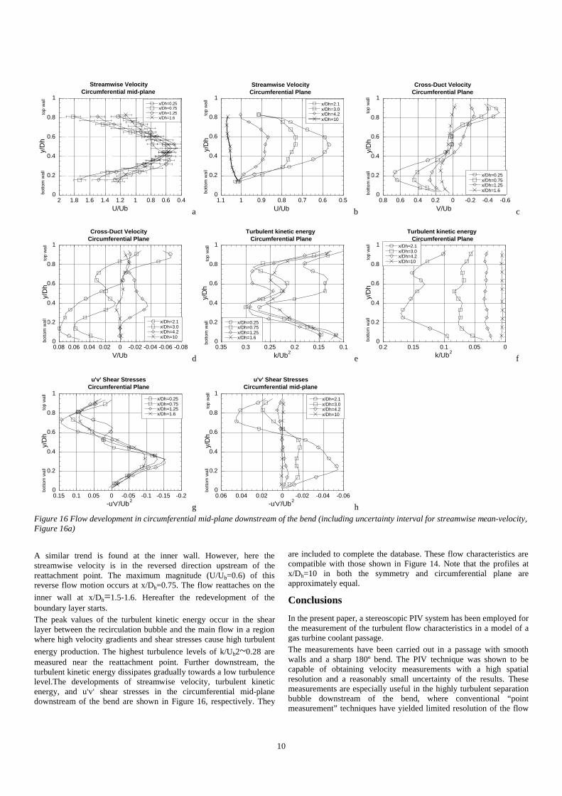
hFigure 16 Flow development in circumferential mid-plane downstream of the bend (including uncertainty interval for streamwise mean-velocity,Figure 16a)

A similar trend is found at the inner wall. However, here thestreamwise velocity is in the reversed direction upstream of thereattachment point. The maximum magnitude (U/Ub=0.6) of thisreverse flow motion occurs at x/Dh=0.75. The flow reattaches on the

inner wall at x/Dh=1.5-1.6. Hereafter the redevelopment of theboundary layer starts.The peak values of the turbulent kinetic energy occur in the shearlayer between the recirculation bubble and the main flow in a regionwhere high velocity gradients and shear stresses cause high turbulent

energy production. The highest turbulence levels of k/Ub2~0.28 aremeasured near the reattachment point. Further downstream, theturbulent kinetic energy dissipates gradually towards a low turbulencelevel.The developments of streamwise velocity, turbulent kineticenergy, and u’v’ shear stresses in the circumferential mid-planedownstream of the bend are shown in Figure 16, respectively. They

are included to complete the database. These flow characteristics arecompatible with those shown in Figure 14. Note that the profiles atx/Dh=10 in both the symmetry and circumferential plane areapproximately equal.

Conclusions

In the present paper, a stereoscopic PIV system has been employed forthe measurement of the turbulent flow characteristics in a model of agas turbine coolant passage.The measurements have been carried out in a passage with smoothwalls and a sharp 180º bend. The PIV technique was shown to becapable of obtaining velocity measurements with a high spatialresolution and a reasonably small uncertainty of the results. Thesemeasurements are especially useful in the highly turbulent separationbubble downstream of the bend, where conventional “pointmeasurement” techniques have yielded limited resolution of the flow

11

characteristics. The data acquisition rate was high and thus allowedfor the investigation of the flow in a complex geometry where manymeasurement planes are required to obtain a comprehensiveunderstanding of the flow phenomena and a large database to evaluateturbulence models for CFD codes. From the statistical distribution ofthe velocity components, the mean-velocity field and turbulenttransport of the flow were calculated. The velocity fields werearranged on a regular grid and can therefore ideally be used toevaluate CFD simulations.As expected, the PIV measurements showed that the flow in thecoolant passage was characterized by the development of a strongDean-type secondary flow in the bend. The secondary flow consistedof two counter rotating vortices that transport fluid in the bend centerfrom the inner wall towards the outer. Close to the sidewalls, thesecondary flow was convected to the inner wall. Downstream of thebend exit, a large separation bubble existed on the inner wall. In thesymmetry plane, the flow reattached at 1.5-1.6 hydraulic diametersfrom the bend exit and towards the sidewalls the reattachment lengthincreased. In both outer corners, zones of recirculating flow weremeasured. The secondary flow caused a strong impingement of theflow on the outer walls at the bend exit.Because of the space limitations, only a fraction of the results thatwere obtained by the measurements could be presented in this paper.For a more complete database, the readers are referred to the seniorauthor, J.S.

Acknowledgement

This study was supported by ABB Corporate Research, Ltd.,Switzerland.

References

P.J. Bryanston-Cross, P.J. Towers, C.E. Judges, S.P. Harasgama,1991, “The Application of Particle Image Velocimetry in a ShortDuration Transonic Annular Turbine Cascade,” ASME paper 91-GT-221S.M. Chang, J.A.C. Humphrey, A. Modavi, 1983, “Turbulent Flow ina Strongly Curved U-Bend and Downstream Tangent of SquareCross-Sections,” PCH PhysicoChemical Hydrodynamics, Vol. 4, No.3, pp. 243-269S.C. Cheah, H. Iacovides, D.C. Jackson, H. Li, B.E. Launder, 1994”,LDA Investigation of the Flow Development Through Rotating U-Ducts,” ASME paper 94-GT-226S.V. Ekkad, J.C. Han, 1995,”Local Heat Transfer Distribution Near aSharp 180º Turn of a Two-Pass Smooth Square Channel Using aTransient Liquid Crystal Image Technique,” J. Flow Vis. Image Proc,.Vol. 2, pp. 285-297S.P. Gogineni, D.D Trump, R.B. Rivir, D.J. Pestian, 1996, “PIVMeasurements of Periodically Forced Flat Plate Film Cooling Flowswith High Free Stream Turbulence,” ASME paper 96-GT-236Ian Grant (editor), 1994, “Selected Papers on Particle ImageVelocimetry,” Spie Milestone Series, Vol. MS 99J.C. Han, P. Zhang, 1991, “Effect of Rib-Angle Orientation on LocalMass Transfer Distribution in a Three-Pass Rib-Roughened Channel,”Journal of Turbomachinery, Vol. 113, pp. 123-130J.C. Han, P.R. Chandra, S.C. Lau, 1988, “Local Heat/Mass TransferDistributions Around Sharp 180º Turns in Two-Pass Smooth and Rib-Roughened Channels,” ASME Journal of Heat Transfer, Vol. 110, pp.91-98K.D Hinsch, 1995, “Three-Dimensional Particle Velocimetry,” Meas.Sci. Technol. Vol. 6, pp. 742-753H. Iacovides, D.C. Jackson, H. Li, G. Kelemenis, B.E. Launder, K.Nikas, 1996, “LDA Study of the Flow Development through an

Orthogonally Rotating U-Bend of Strong Curvature and RibRoughened Walls,” ASME paper 96-GT-476R.W. Johnson, B.E. Launder, 1985, “Local Heat Transfer Behaviourin Turbulent Flow Around a 180 deg Bend of Square Cross Section,”ASME paper 85-GT-68B. Lakshminarayana, 1996, Fluid Dynamics and Heat Transfer ofTurbomachinery, John Wiley & Sons, Inc.T.M. Liou, C.C. Chen, 1997, ”LDV Study of Developing Flowsthrough a Smooth Duct with a 180 deg Straight-Corner Turn,” ASMEpaper 97-GT-283L.M. Lourenco, 1988, “Some Comments on Particle ImageDisplacement Velocimetry,” Von Karman Institute for FluidDynamics, Lecture Series 1988-06D.E. Metzger, M.K. Sahm, 1986, “Heat Transfer Around Sharp 180ºTurns in Smooth Rectangular Channels,” Journal of Heat Transfer,Vol. 108, pp. 500-506A.K Prasad, R.J Adrian, 1993, “Stereoscopic Particle ImageVelocimetry Applied to Liquid Flows,” Experiments in Fluids, Vol.15, pp. 49-60J. Schabacker, A. Bölcs, 1996, “Investigation of Turbulent Flow byMeans of the PIV Method,” Paper presented at the 13th Symposium onMeasuring Techniques for Transonic and Supersonic Flows inCascades and Turbomachines, Zurich, Switzerland, September 5-6D. Tisserant, F.A.E. Breugelmans, 1995, “Rotor Blade-to-BladeMeasurements Using Particle Image Velocimetry,” ASME paper 95-GT-99D.G.N. Tse, G.D. Steuber, 1997, “Flow in a Rotating SquareSerpentine Coolant Passage with Skewed Trips,” ASME paper 97-GT-529J. Westerweel, F. T. Nieuwstadt, 1991, “Performance Tests on 3-Dimensional Velocity Measurements with a Two-Camera DigitalParticle-Image-Velocimeter,” Laser Anemometry, Vol. 1, pp. 349–355