PIV Measurements Applied to Hydraulic Machinery ...cdn.intechopen.com/pdfs/37153/InTech-Piv... ·...

3

PIV Measurements Applied to Hydraulic Machinery: Cavitating

and Cavitation-Free Flows

Gabriel Dan Ciocan and Monica Sanda Iliescu Université Laval, Laboratoire de Machines Hydrauliques

Canada

1. Introduction

Hydraulic machinery is an ideal field of application for Particle Image Velocimetry in terms

of scientific interest, due to the complexity of the flow behaviour and to the need of detailed

unsteady experimental data simultaneously recorded over large sections of the flow field.

Within the same machine, a whole range of phenomena are encountered in the different

components: wake patterns, separation, rotating vortex structures, vortex breakdown, etc.

The unsteady interactions between the stationary and rotating frames, both upstream and

downstream the runner, contribute to the efficiency loss. The generated quasi-periodic

fluctuations overlay onto the average flow field, which may be symmetrical or not, issuing

an unpredictable dynamic behaviour with respect to the operating regime. Whilst the

intrinsic parameters of the local phenomena (e.g. sheared flow mixing length) vary, the flow

topology may be modified drastically for conditions situated relatively close to one another

in terms of head, flow rate and efficiency. The mapping of the unsteady velocity fields and

corresponding turbulence levels is thus an essential tool in the analysis of these complex

phenomena. The PIV technique opens large perspectives in the analysis of internal flows in

hydraulic machinery, providing valuable insight towards an extensive understanding of the

underlying physical mechanisms. Nevertheless, the use of PIV systems in this context is one

of the most challenging applications, due to the structural constrains related to the optical

access to the measurement areas, to the spatial and temporal scales of the phenomena that

are to be investigated, two phase flow structure in cavitating regime and also due to the

industrial aspects of the application.

In this book chapter it is proposed for presentation a development for hydraulic machines,

based on our extensive experience and on the current bibliography in the field. The focus

will be on two directions: rotor-stator interactions and two-phase flows in hydraulic

turbines taking into account flow periodicity, turbulence and cavitation.

The research on hydraulic machinery is mainly performed on reduced scale models. The

internal geometry needs to be respected because it is essential for the step-up of flow

phenomena taking place on the model to actual prototype conditions. Furthermore, the

model operation conditions must comply with the IEC 60193 Standard, which rules the

www.intechopen.com

The Particle Image Velocimetry – Characteristics, Limits and Possible Applications

52

methodology for model acceptance testing of hydraulic turbines, storage pumps and pump-

turbines, and provides guidelines for the model-to-prototype transposition.

Fig. 1. Cross-section of a Francis turbine scale model

Fig. 2. Development of a cavitating helical vortex downstream the runner of a Francis turbine at partial load

An example of hydraulic geometry of a medium-head radial turbine is presented in Fig. 1. For this kind of turbine, the runner has constant-pitch fixed blades and the guide vanes are adjustable. The environment around the machine is also complex because it concerns the operating elements of the machine, supports of the test bench, model instrumentation to operate the machine. The working fluid is water; also thus optical interfaces are required for measurements based on imaging techniques. Their design must take into account the internal geometry of the model, while minimizing distortion.

Another major topic to be considered is the flow topology and diversity, with various unsteady phenomena taking place: wake propagation, vortex breakdown and machine-circuit resonance, rotor-stator interaction, runner flow behaviour. The 2D PIV and 3D PIV, in cavitation-free or two phase flow are the ideal tool to characterize these complex flows – see Fig. 2.

The proposed chapter covers all aspects of the development of a stereoscopic PIV experiment for the investigation of unsteady flows in hydraulic machinery, illustrated by the main applications of the authors' experience (see bibliography). The following topics are discussed in details:

www.intechopen.com

PIV Measurements Applied to Hydraulic Machinery: Cavitating and Cavitation-Free Flows

53

Interface design criteria and optimisation of the optical access taking into account local optical distortions and perspective effects;

Calibration devices and practical procedures for accuracy assessment;

Experiment setup for measurements in the static and rotating frames: synchronisation of the acquisition with the predominant physical phenomena; adjustment of the acquisition parameters with respect to the local flow conditions and to the global operating range of the machine;

Requirements for image quality optimisation in 2D/3D-PIV experiments in single and two-phase flows: uniformization of the laser illumination in the measuring section, solutions to prevent localised reflections in the active viewing area, specificities related to measurements in two phase flows such as background illumination;

Image processing in two-phase flows: filtering methodology and morphological operations to extract the relevant flow features;

Data processing tools to determine the 3D velocity fields, with emphasis on particle detection on textured backgrounds and related masking techniques;

Accuracy study and validation of measurement results, in terms of velocity fields and geometrical features extracted in two-phase flow conditions;

Physical analysis of the flow (wake propagation, vortex core detection techniques, reconstruction of vapours volume, etc).

To conclude the chapter, best practice guidelines are provided for the setup of PIV experiments in hydraulic turbo-machinery, comparatively in single-phase flows and cavitation conditions.

All this works are done in the frame of PhD works of the authors: (Ciocan 1998) performed at Institute National Politechnique de Grenoble, France and (Iliescu 2007) performed at Ecole Polytechnique Federale de Lausanne, Switzerland. Other ulterior developments were performed (Tridon et al. 2008), (Tridon et al. 2010), (Gagnon et al. 2008), (Beaulieu et al. 2009) and (Houde et al. 2011) in collaboration or under the coordination of the authors.

2. General setup for hydraulic machines applications

2.1 General experimental set-up

A Dantec MT 3D-PIV system is used for measuring the three-dimensional unsteady velocity fields. The equipment presented herein corresponds to a classical medium-frequency PIV system. The system components belong to four categories of devices: illumination, particles introduced in the flow, image recording and data processing unit – see Fig. 3.

2.2 Illumination system

Two laser units with individual power supplies and cooling loops deliver a high-energy laser beam, which is transformed into a plane for locally illuminating the flow seeded with tracer particles.

The laser has an Yttrium Aluminum Garnet crystal, doped with triply ionized Neodymium, as lasing medium (Nd:YAG). While stimulated with a flash lamp, it emits photons of 1064 nm wavelength. The infrared output light is converted to the visible spectrum by frequency doubling with a birefringent crystal, up to the green radiation wavelength, 532 nm. The laser delivers pulses of 250 μs at a frequency of 8Hz. A Q-switch mechanism releases only 8 ns

www.intechopen.com


54

Fig. 3. Typical layout of a 3D-PIV system

out of the total pulse duration, thus producing a stroboscopic effect on the particles in the test area. For obtaining the desired delay between two pulses, two laser cavities with the same characteristics are used. Thus, the time interval between two successive impulses can be easily adjusted within 1 μs ÷ 100 ms range, depending on the local flow characteristics or the phenomenon, which is to be captured. The characteristics of the illumination system used for the current experiments are summarized in Table 1.

Type NewWave Gemini

Peak energy 60 mJ Pulse duration 8 ns

Lasing medium

Nd:YAG Power 25 MW Pulse repetition rate 8 to 20 Hz

Output wavelength

532nm Beam diameter

6mm Pulse separation rate 300 ns to 300 ms

Table 1. Laser unit specifications

For facilitating the optical access to the test section, the laser beam is transmitted through an articulated light guide with high transfer ratio and resistant to the high laser energy employed in water experiments. The characteristics of the beam guide are given in Table 2.

Type 5 flexible joints mirrors

Optical transmission >90%

Maximum input pulse energy 500 mJ for 10 ns pulse and 6-12 mm beam

Maximum input beam diameter 12 mm

Table 2. Beam-guiding arm specifications

A beam expander mounted at the end of the arm transforms the input laser beam into a light sheet. A series of lenses allow adjusting the thickness and divergence angle of the laser sheet. The characteristics of the optics assembly are given in Table 3.

www.intechopen.com


55

Narrow angle lens opening 20°Wide angle lens opening 40°Thickness adjuster compression factor for 2D PIV 0.67Thickness adjuster expansion factor for 3D PIV 1.5Focus lens focus adjuster module

Table 3. Laser sheet optics assembly specifications

2.3 Image recording

The enlighten field is visualized by two double-frame progressive scan interline CCD cameras, with an active matrix of 1280x1024 with 8 bit depth, see Table 4. The active area of light-sensitive cells is doubled by a second array of storage cells, for increasing the data transfer rate. The acquisition frequency in double-frame mode is 4.5 Hz. The CCD chip is cooled, which gives a higher sensitivity and signal-to-noise ratio enhancement in low lighting conditions. Two Nikon objectives with focal length of 24mm and 60mm are used depending on the geometrical characteristics of the camera setup. measurement area dimensions and optical path.

CCD chip

cooling system, anti-blooming protection, pixels binning

Active area 1280 x 1024 Resolution 8-12 bit Pixel width and pitch

3.4μm x 6.7μm Frame rate 4.5 Hz in double-frame mode

Table 4. CCD camera specifications

2.4 Acquisition control and data processing

The control and synchronization of the laser, cameras and external trigger input, as well as the raw vector field processing, are realized with a specific processor, Dantec MT’s FlowMap2200. The main advantage is the integrated correlator unit, which performs real-time raw vector maps processing by a cross-correlation technique applied on the double-frame images. In this way a qualitative vector field validation can be rapidly performed during acquisition.

Dantec MT’s FlowManager software version 4.5, along with 3D-PIV software module, have been used for data acquisition, validation and processing. Data post-processing and visualization tools are realized in Matlab.

2.5 Seeding

Spherical particles in borosilicate glass, are used as flow tracers; a silver coating improves their scattering characteristic. The relative density of 1.4 against the water one and the average size of 10m allow these particles to accurately follow the flow. Their refractive index is 1.52. The melting point is high, 740°C, which makes them suitable for a broad range of applications.

2.6 Calibration

For the correct evaluation of the 3D displacement of the particles, a mapping of the measurement volume onto the two cameras' images and the definition of the overlapping zone of the two fields of view are necessary.

www.intechopen.com


56

The camera calibration consists in defining the coefficients of a mathematical model that relates the real spatial locations in the measurement plane to the corresponding positions in the recording plane. This model includes the geometrical and optical characteristics of the cameras set-up, taking into account the optical distortions due to perspective imaging, lens aberrations, interposed media with different refractive indices. The images of a plane target with equally spaced markers, moved in five transversal positions (corresponding to the laser sheet thickness) are stored to have volume information. The corresponding positions of the points in all the image plane allows to determine the optical transfer function by a least squares fitting algorithm.

2.6.1 Optical distortion correction

For the optical access of the cameras and of the laser, the test model is equipped with

polymethyl methacrylate (PMMA) windows, with a refractive index of 1.44. The inner face

of the windows follows the hydraulic profile of the test model, while their external face is

flat, for minimizing the optical distortions. The optical interfaces used for the PIV

measurements in the cone will be detailed in the next paragraphs.

The Scheimpflung correction is applied for perspective imaging rectification. It consists in

rotating the CCD plane relatively to the lens plane for reducing the perspective effect by

balancing the optical path difference between points near and far away from the camera

axis. The focus plane, lens plane and CCD sensor plane are made coincident using a

mechanism which allows individual rotation of these components.

The angle at which the CCD chip plane needs to be tilted about the lens plane can be

calculated with the camera's focal length and its geometrical position, i.e. the camera tilt

angle and the distance from the lens to the measurement plane. In our case, this value can

only be used as a rough approximation, because the optical path is distorted while passing

through air, PMMA and water. The final adjustment is then realized by compensating the

blur on the lateral edges of the image and bringing the entire view into focus.

2.6.2 Optical transfer functions

The optical path from the measurement zone to the camera crosses 3 media with different

refractive indices: water 1.33. PMMA 1.44 and air 1. In our particular case, the optical

windows are not parallel to the cameras’ plane. To correct the optical distortion between the

measurement zone and the corresponding image, two analytical functions have been tested:

direct linear transform :

11 12 13 14

21 22 23 24

0 31 32 33 341

x

y

Xk A A A A

Yk A A A A

Zk A A A A

(1)

3rd order polynomial for the XY directions in the plane of the target and parabolic in the out-of-plane direction Z:

www.intechopen.com


57

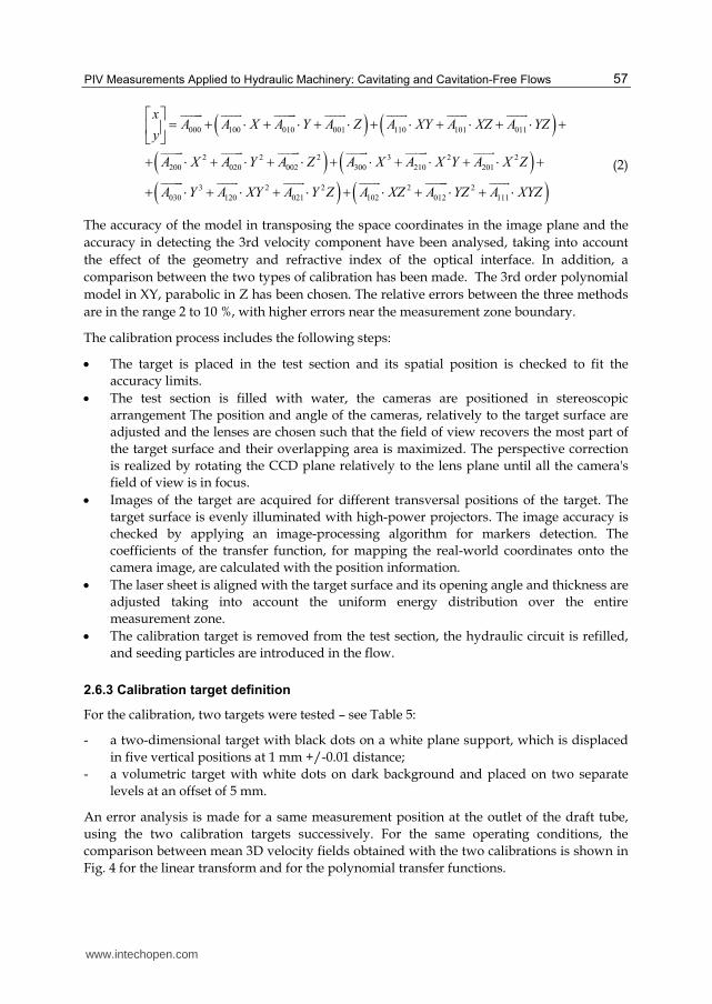
000 100 010 001 110 101 011

2 2 2 3 2 2

200 020 002 300 210 201

3 2

030 120 021

xA A X A Y A Z A XY A XZ A YZ

y

A X A Y A Z A X A X Y A X Z

A Y A XY A

2 2 2

102 012 111Y Z A XZ A YZ A XYZ

(2)

The accuracy of the model in transposing the space coordinates in the image plane and the

accuracy in detecting the 3rd velocity component have been analysed, taking into account

the effect of the geometry and refractive index of the optical interface. In addition, a

comparison between the two types of calibration has been made. The 3rd order polynomial

model in XY, parabolic in Z has been chosen. The relative errors between the three methods

are in the range 2 to 10 %, with higher errors near the measurement zone boundary.

The calibration process includes the following steps:

The target is placed in the test section and its spatial position is checked to fit the

accuracy limits.

The test section is filled with water, the cameras are positioned in stereoscopic

arrangement The position and angle of the cameras, relatively to the target surface are

adjusted and the lenses are chosen such that the field of view recovers the most part of

the target surface and their overlapping area is maximized. The perspective correction

is realized by rotating the CCD plane relatively to the lens plane until all the camera's

field of view is in focus.

Images of the target are acquired for different transversal positions of the target. The

target surface is evenly illuminated with high-power projectors. The image accuracy is

checked by applying an image-processing algorithm for markers detection. The

coefficients of the transfer function, for mapping the real-world coordinates onto the

camera image, are calculated with the position information.

The laser sheet is aligned with the target surface and its opening angle and thickness are

adjusted taking into account the uniform energy distribution over the entire

measurement zone.

The calibration target is removed from the test section, the hydraulic circuit is refilled,

and seeding particles are introduced in the flow.

2.6.3 Calibration target definition

For the calibration, two targets were tested – see Table 5:

- a two-dimensional target with black dots on a white plane support, which is displaced

in five vertical positions at 1 mm +/-0.01 distance;

- a volumetric target with white dots on dark background and placed on two separate

levels at an offset of 5 mm.

An error analysis is made for a same measurement position at the outlet of the draft tube,

using the two calibration targets successively. For the same operating conditions, the

comparison between mean 3D velocity fields obtained with the two calibrations is shown in

Fig. 4 for the linear transform and for the polynomial transfer functions.

www.intechopen.com


58

Plane target

Volumetric target

active area 200x200 mm 270x190 mm

dot spacing 5 mm 20 mm

dot diameter 2 mm 5 mm

reference marker diameter 2.7 mm 7 mm

axis marker diameter 1.3 mm 5 mm

Level spacing - 4 mm

Table 5. 2D and volumetric calibration targets dimensions

Fig. 4. Relative error for calibration with the 2D and the 3D targets, in the case of linear (top row) and polynomial (bottom row) transfer functions

2Dtarget 3Dtarget

2Dtarget

100 %C C

C

(3)

The high error values obtained for the comparison between the measurements obtained with the two targets shows that the 3D target cannot be used in our configuration. The reasons, which explain this difference of accuracy, are the following:

for the volumetric target, the dots positions cover only 2 traverse planes on the vertical direction (Z), thus only a linear correction can be performed along Z, and the larger spacing of the dots results in a lack of information for the in-plane positions;

the position of the cameras is not symmetrically placed relatively to the target plane, by accessibility reasons;

www.intechopen.com


59

the optical access window is not parallel to the image plane;

the tangential velocity component (perpendicular to the main flow direction) is small compared with the axial flow velocity. only 10%, and thus the error is amplified.

Taking into account these considerations, the final choice was to use the 2D target, with a spatial resolution of 5mm for the in-plane positions and 1mm in the out-of-plane direction.

2.6.4 Target positioning system

A slight displacement of the target during calibration has been noticed. In this context, a theoretical and an experimental study have been performed on the stability of the target in the fluid medium, both in rotation and in translation, and on its influence on the measurement accuracy.

Target rotation

Denoting C the velocity in the reference frame OXYZ and C' the velocity in a frame rotated by an angle δ around one of the axes, the relative error for each component is:

100 [%]

C C

C 1 100 [%]

C

C

(4)

- rotation around Ox:

cos

sin

y zy

z yz

C CC

C CC;

1 1 cos

1 sin

z yy

y zz

C C

C C

(5)

- rotation around Oy:

cos

sin

x x z

z xz

C C C

C CC;

1 1 cos

1 sin

x z x

z x z

C C

C C

(6)

- rotation around Oz:

cos

sin

x x y

y xy

C C C

C CC;

1 1 cos

1 sin

x y x

y x y

C C

C C

(7)

Thus the error depends only on the rotation angle and velocity components ratio. These ratios vary in the range [0 1] for Cz/Cy, [1 20] for Cz/Cx, and [1 30] for the in-plane components Cy/Cx. The relative errors for rotation around each axis are given in Fig. 5, for angles ranging between 0 and 2°. The black line denotes 3% error limit.

For rotation around the OX axis:

Cy is sensitive if Cz<Cy, but the admissible angle drops under 1° if Cz>Cy;

Cz is very sensitive to rotation if Cz<<Cy, but for Cz~=Cy the tolerance approaches 1.7°;

Cz is the most sensitive component, which gives a tolerance of 0.1-0.2°.

For rotation around the OY axis:

www.intechopen.com


60

Cx is the less sensitive if Cz<Cx (tolerance >2°), but the limit decreases under 0.2° if Cz>>Cx, slowly until Cz=3.5Cx (1.7° to 0.5°) and steeply as the ratio Cz/Cx increases;

Cz is very sensitive to rotation if Cz<Cx (limit 0.1°), but for Cz>>Cx the tolerance exceeds 1.7°;

Cx is the most sensitive component, being the smallest, which gives a tolerance of 0.2°.

For rotation around the OZ axis:

Cx is more sensitive as the ratio Cy/Cx increases;

Cy is almost insensitive if Cy>Cx;

Cx is the most sensitive component, tolerance 0.1°.

Fig. 5. Relative error for an accidental target rotation during calibration

www.intechopen.com


61

The transversal and out-of-plane velocity components (Cx and Cz) are the most sensitive to accidental rotation of the target during calibration, imposing a limit of 0.1° in rotation about the three axes.

Target transversal displacement

The necessary resolution of the target displacement in the out-of-plane direction has been evaluated by accuracy analysis for calibrations with 1 mm and 0.5 mm spacing between successive positions of the target along the Z axis.

1mm 0.5mm

1mm

100 %C C

C

(8)

The error distributions show that the uncertainty does not exceed 3% for the velocity components in the cross-section plane, Cx and Cz, and is smaller than 0.5 % for the component in the main flow direction, Cy. On the other hand, the polynomial transfer function linear in Z and parabolic in XY is very sensitive to the target positions spacing in the out-of-plane direction, reaching 5% for the small velocity components Cx and Cz. The calibration with 1 mm target displacement in the out-of-plane direction has been chosen for the PIV measurements in most of the turbine sections. The offset was reduced to 0.5mm in configurations where drastic tolerances were required for the 3rd velocity component.

Target traversing system

A specific system for placing the target inside the draft tube has been developed. For an uncertainity of 3% on the velocity field measurement, the tolerances are 0.1° in rotation and 0.01 mm for the relative target displacement in the out-of-plane direction.

2.7 Acquisition parameters

A typical PIV experiment procedure consists in setting several acquisition parameters, choosing and testing the trigger signal, acquiring the raw image and/or velocity data, validating the vector field, calculating the 3rd velocity component and finally data output.

The parameters that need to be adjusted for each measurement setup are:

- image quality – laser energy level and camera aperture settings; - seeding particles density in the measurement area; - spatial resolution – dimensions of the analysis window; - time interval between successive frames; - number of unsteady acquisitions.

2.7.1 Image quality

For the CCD camera used in this experiment, the first frame's exposure takes up to 132 μs, while the second frame is exposed during the entire read-out sequence of the first frame, 111 ms. It means that, for short time delays between laser pulses, the background gray level on the second frame will increase sensibly. In order to broaden the dynamic range, the ambient light level is set to minimum during the data acquisition. As the time delay varies according to the local flow field characteristics, the laser's energy level is balanced for each experiment, in order to reach uniform brightness on both images. Moreover, the cameras are equipped with high-pass filters for the emission wavelength of the laser: 532 +/- 5 nm.

www.intechopen.com


62

Another important topic is the uneven energy distribution along the laser sheet, which can have several causes:

- non-uniform Gaussian energy distribution over the beam cross-section; - misalignment of the internal mirrors of the light-guide; - slight rotation of the sheet-forming optics against the thickness adjuster; - lens aberrations; - bad focus of the laser sheet, which leads to thickness variation over the test section; - interface geometry, which can lead to important distortions depending also on the

refractive index of the material.

All these parameters are taken into account and adjusted accordingly for each measurement setup, prior to data acquisition.

2.7.2 Spatial resolution

The measurement zone is divided in small analysis areas, for which a local velocity is calculated with the mean displacement of seeding particles between two successive frames, and the vector's application point is chosen at the center of the area. This grid defines the spatial resolution of the PIV measurement in the 2D case.

In a 2D configuration, the spatial resolution would be given by the distance between two successive vector anchor points in pixels, divided by the scale factor pixels/mm. If a linear dependence exists between the CCD chip dimensions and the measurement zone dimensions, then the scale factor depends on the field of view, on which the camera is focused, i.e. the aperture setup and the optical characteristics of the encountered media.

In a stereoscopic setup, the correspondence image – field of view is not linear anymore, because of the geometrical and perspective distortions due to camera setup. The velocities are calculated on a grid defined on the common zone of the two fields of view, by applying the calibration relationship on the neighboring vectors in both 2D fields, thus solving a linear or nonlinear system of four equations with three unknowns.

The spatial resolution is chosen such as the interpolation bias has a minimum influence on the vector value uncertainty – 2.4x2.5x3mm.

2.7.3 Seeding density

For a measurement to be successful, a minimum of two matching particles should be present in the analysis areas on both frames. According to the Nyquist criterion, the average number of correlated particles in the analysis window should not exceed five. This can be verified statistically checking the overall distribution of the correlation peaks width, which corresponds to the number of matching particle pairs in the correspondent analysis areas. It is checked that the average value fits within 3 – 5 for each measurement setup.

For the instantaneous velocity fields it is very difficult to insure a homogeneous seeding distribution of particles in all interrogation windows, particularly in measurements zones with strong velocity gradients or vortices. To improve the particles traceability, an overlapping of 25% of the analysis areas has been considered. The lack of particles or bad correlations is accounted for during vector field post-processing by correlation peak height and vector size criteria.

www.intechopen.com


63

2.7.4 Time interval

The time delay between two laser pulses must be adapted to the local characteristics of the flow. The prior knowledge of the local velocity range and flow field structure is useful for setting an initial guess for the time delay setting.

The time interval must be chosen as small as possible to insure a good sensitivity for small particle displacements, to fit into the limits of the sub-pixel interpolation resolution, and as large as possible that the particle remains in the laser sheet width and within the interrogation area limits during the two camera exposures. The time delay optimization is particularly challenging in zones with strong velocity gradients, such as backflow zones or vortices. Typical values in our experimental conditions are between 50 – 300 μs.

2.7.5 Synchronization

In a turbine, the runner rotation forces the periodic behavior of the flow. One way to reconstruct the shape of a signal acquired by an unsteady measurement technique is the phase-locking, i.e. triggering the acquisition with a reference signal at different time delays within the event's period. In our specific case, the reference signal is the runner frequency, delivered by an optical encoder mounted on the shaft. The optical encoder delivering a signal per rotation has been used for acquisition synchronization for the operating points near the best efficiency conditions.

The PIV laser can be operated in window triggering mode, which means that the laser burst can be advanced if the trigger signal comes within a fixed time interval before the expected bursting moment. Although, the acquisition frequency is limited by the camera frequency in double-frame mode: 4.5 Hz. This slow-down only influences the experiment duration for achieving convergence, since the acquired signal is sampled at the same phase.

The synchronization of the laser and cameras with the external event is insured by the processor unit. The timing diagram is presented in Fig. 6.

Fig. 6. Timing diagram for the PIV data acquisition and synchronization with an external frequency

2.8 Data validation and post-processing

2.8.1 Data validation criteria

The raw 2D vector fields resulting from cross-correlation can contain velocity values that have not been correctly detected, which bias the subsequent statistical analysis. A series of validation methods have been used for removing the outliers:

www.intechopen.com


64

- Area masking – a digital mask is applied on the zones covered by obstacles in the field of view of one or both cameras and the corresponding vectors are eliminated;

- Correlation quality validation – the first highest peak in the correlation plane is considered as the signal peak, while the second one comes from the image noise. The signal-to-noise ratio should be about 20%. The first peak's height depends on the seeding density in the interrogation area, as well as on the image quality, i.e. uniform illumination and good spot-background contrast;

- Range validation – depending on the local characteristics of the flow field, the vector's length or its components may be limited;

- Moving average – through an iterative process, a vector is replaced with the average of its m×n neighbors,

1 1

2 2

1 1

2 2

1( , ) ( , )

m nx y

m ni x j y

C x y C i jmn

(9)

if the difference between them exceeds a percentage of the maximum difference in the vector field,

,

) max )( , ) - ( , ( , ) - ( ,x y

C x y C x y C x y C x y (10)

This filter has a smoothing effect, thus it is used with caution when strong velocity gradients are present.

2.8.2 Validation with LDV data

Systematic errors, coming from calibration accuracy, image quality, cross-correlation, vector validation, interpolation for 3rd component calculation, repetitiveness and reference frame transform, have been addressed in the previous chapters and are evaluated to 3% of the mean velocity value.

Fig. 7. PIV-LDV data comparison in the inlet and outlet sections of the cone of the draft tube

www.intechopen.com


65

However, even if all of the previous considerations are fulfilled, the uncertainty of 3% holds only if the optical deformations of the image, due to the optical interfaces, are sufficiently small to be corrected by the polynomial function. To check this condition, a comparison was made between the PIV measurements and LDV measurements see Fig. 7. In this way, the global accuracy of the PIV measurement in this configuration is assessed.

The similar spatial resolution for the two measurement systems does not induce a supplementary error source: the measurement volume for the PIV measurement is a parallelepiped of 2.4 x 2.4 x 3 mm3 and for the LDV measurement is an ellipsoid of 2.4 x 0.2 x 0.2 mm3. The result shows a good agreement, within 3%, for the entire PIV measurement field.

3. PIV measurements for rotor-stator interaction investigations

3.1 Phenomenology in pumps and turbines

The rotor-stator interaction is a complex set of phenomena stemming from the nature of the machine itself – such as periodic rotation instabilities and blade interactions – (Ciocan et al. 1996). The unsteady phenomena related to the interactions between the static and mobile parts often affect machine efficiency. Under the influence of periodic constraints, pressure and velocity fluctuations generate stress fluctuations and induce vibrations that contribute to material fatigue of the components and may also issue hydraulic noise. Blade interactions differentiate from other phenomena encountered in turbomachinery by their independence of the operation conditions. Whichever the turbomachine type and its operating regime, these interactions occur under the form of an unsteady secondary flow superposed onto the average stationary flow.

In hydraulic machinery (pumps, turbines and pump-turbines), the following phenomena, briefly described hereafter, are to be considered: potential interactions, wake interactions, von Kármán vortex interactions, three-dimensional viscous interactions and instabilities of the efficiency curve:

Potential interactions are characterized by a non-uniform distribution of the unsteady pressure field in the gap between the static and rotating parts (e.g. guide-vanes and runner). This type of interaction has a non-convective character and its influence extends towards upstream as well as downstream the gap – see (Mesquita et al. 1999).

Wake interactions are determined by the non-uniformity of the velocity profiles downstream blade casades (e.g. at the runner outlet in a centrifugal pump) – see (Iliescu et al 2004). The main source of this non-uniformity is the shear layer created at the trailing edge by the combination of the boundary layers developed on the blade's pressure and suction sides. The velocity defect decays due to viscous effects, and its mixing length depends on the blade shape, local flow velocity and turbulence level. This phenomenon is of purely convective nature and it has no influence upstream its location.

Von Kármán vortex street interactions take place downstream blade cascades with blunt trailing edge, in low turbulence conditions. Their shedding frequency is generally expressed in terms of Strouhal number, which depends on the characteristic blade dimensions and on the local flow velocity. If the vortex shedding frequency reaches resonance with the natural frequencies of the system, it may lead to structural vibrations.

www.intechopen.com


66

Viscous three-dimensional interactions are secondary flows in the inter-blade channels, such as passage vortex, corner vortex, horseshoe vortex and tip gap vortices. They are closely related to the shape of the different hydraulic passages, which force variations in the flow direction and local modifications of the boundary layer topology. It is likely that these phenomena are the main contribution to local efficiency loss in specific areas of the operating range. Certain machines (pumps and pump-turbines) often exhibit an unstable zone of the efficiency characteristic, with discontinuities of up to 3%, accompanied or not by hysteresis – see (Ciocan et al. 2001).

The accurate prediction of these phenomena is essential at the design stage, and PIV measurements are the ideal tool to investigate them. The first experiment set up to analyze these interactions is described in (Ciocan et al. 2006).

3.2 Experimental set-up

2D-PIV measurements have been performed in the guide-vanes channel of a pump-turbine

model of specific speed nq=66. Several operating conditions were investigated in both pump

and turbine regimes, covering a large portion of the operating range.

To obtain the velocity field evolution in the guide-vane channels, the measurement section

has been chosen such as to cover the space between two wicket gates. This area is

determined by the 'visibility' zone, i.e. the area which is accessible by a laser sheet through

windows embedded in the spiral casing walls – see Fig. 8. Two stay vanes that obstructed

the visual access to the measurement section have been removed. Views through two

separate windows were necessary in order to cover the full extent of the measurement

domain.

Laser

beam

90 %

10 % 30 % 50 % 70 %

Camera

Laser plane (9°)

Mirror

Fig. 8. Top and side views of the measurement sections and laser sheet positions for the PIV experiment in the guide-vanes channel of a pump-turbine

Five sections have been analyzed along the height of the channel. Considering the important

optical constraints imposed by previous LDV investigations in the same section, the imaging

window was tilted by 9° with respect to the machine's axis. To enable the most adequate

conditions for the PIV experiment, the laser planes were also tilted of 9° in the radial

direction to match the central window level – see Fig. 9.

www.intechopen.com


67

Fig. 9. Overview of the PIV setup. Detail on the right side shows the image reflected by the inclined mirror, as seen from the CCD camera standpoint

To obtain a sharp image with a CCD camera, the focusing plane must be in the plane of the laser sheet. Another requirement for a 2D-PIV experiment is to set the camera imaging axis normal to the measurement plane. To ensure minimum optical distortion, the different interfaces traversed by the scattered light must be smooth and parallel to the laser sheet as well. In the present case, the camera is installed on a mobile support with two degrees of freedom – translation and rotation. Considering the camera's focal length and visual access difficulties, a plane mirror was placed in front of the window to redirect the optical path horizontally towards the camera, as illustrated in Fig. 9.

The mirror must meet high quality standards (flatness of the surface and homogeneity of the reflective coating), to avoid additional errors in the measurement process. The solution adopted for this experiment was a price-quality compromise: Pyrex wafer with ALMGF2

coating, λ/2 flatness. The mirror was mounted on the same support as the camera, aligned at 45° with respect to the lens. The CCD-mirror assembly was oriented parallel to the laser sheet and the support axis was secured horizontally. The final adjustment was made by optimizing the sharpness of the acquired images, with an estimated maximum uncertainty of 0.6°.

Regarding the laser sheet positioning, in a first approach the optical path of the laser sheet was calculated and it was planned to adjust its position in-situ using a device attached to the light-guiding arm. The precision was not satisfactory, thus it has been decided to mark directly the position of the plane directly onto the wicket gates, for each vertical position. The laser sheet contour was traced on the opposite faces of two guide vanes that form a channel. First tests revealed scattering problems on the shroud, runner blades and guide vanes. The issue was corrected by painting these bright metallic surfaces with a matte black dye. Several tests were made to determine the appropriate dye for the intended objectives – reflection attenuation and durability under repeated laser pulse operation. A black permanent marker was chosen.

3.3 Main results

The measurements have been acquired synchronously with the runner rotation, for multiple phase angles corresponding to portions of a single runner inter-blade channel. Ten angular

www.intechopen.com


68

positions were investigated, evenly distributed at 7.2°. For each spatial position, downstream the runner and between the guide vanes, the two dominant velocity components have been measured, corresponding to the radial and tangential directions. The average velocities are calculated with 250 PIV frame pairs by phase.

According to the ergodicity assumption for a stationary flow, the mean velocity was estimated by the temporal mean of the ensemble (eq. 11), and the standard deviation (eq. 12) for each component of the mean velocity is calculated as follows:

( ) /c c i N (11)

² ( ) ² ( 1)c i c N (12)

c(i) – measured instantaneous velocity c – statistical average velocity N – number of samples in each spatial position - standard deviation (rms) of the mean value

Using the rms values, the turbulent kinetic energy can be estimated. Having only two components, it is assumed that isotropy conditions are met, i.e. the rms of the missing component is of the same order of magnitude as the two measured components. Furthermore, the periodic velocity fluctuations (deterministic) are negligible with respect to the turbulent fluctuations (random), thus the specific energy of the turbulent structures in the flow may be calculated using the individual standard deviation of the velocity components. In these conditions, the turbulent kinetic energy can be calculated as follows:

2 234 r tk (13)

k - turbulent kinetic energy for the synchronous velocity component

r - rms of the mean radial velocity

t - rms of the mean tangential velocity

A typical result for the steady velocity field in turbine mode is presented in Fig. 10. For the measured range of operating points, 20% around the nominal flow rate, the guide vanes direct correctly the mean flow towards the runner inlet and back flows or detachment zones have not been observed.

The mean velocity profiles in pump mode, in a guide vanes channel ad mid height, are presented in Fig. 11 for a stable operating condition, while Fig. 12 shows the velocity profiles for an unstable portion of the operating range.

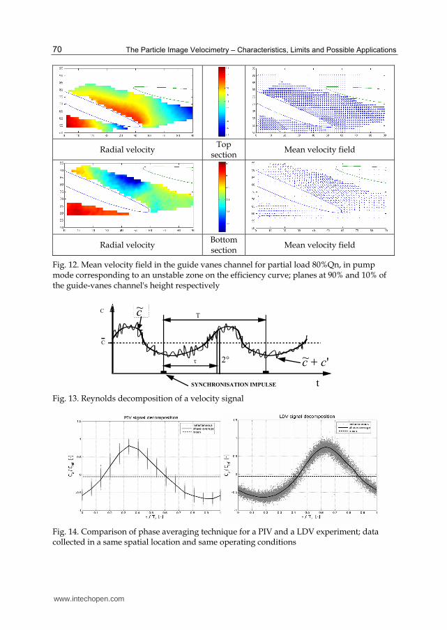
A phase averaging technique is used to analyze the periodic fluctuations synchronuous with

the runner. An optical encoder provides the time basis, as a reference runner position.

According to the Reynolds decomposition scheme (eq. 14), an unsteady velocity field can split

in three parts: the temporal mean of the ensemble c , a periodic fluctuation with respect to the

mean ( )c c and a random turbulent fluctuation 'c . The process is illustrated in Fig. 13. A

comparison between PIV and LDV phase average technique is presented in Fig. 14

( ) ( ) 'c i c c c c (14)

www.intechopen.com


69

Radial velocity

Tangential velocity

Velocity angle

Velocity field

Fig. 10. Mean velocity field in the guide vanes channel for optimum flow rate Qn in turbine mode; mid-channel height; flow direction towards the runner

Radial velocity

Tangential velocity

Velocity angle

Mean velocity field

Fig. 11. Mean velocity field in the guide vanes channel for optimum flow rate Qn in pump mode; mid-channel height; flow direction exiting the runner

guide vane

guide vane

runner inlet

guide vane

guide vane

runner inlet

www.intechopen.com


70

Radial velocity Top

section Mean velocity field

Radial velocity Bottom section

Mean velocity field

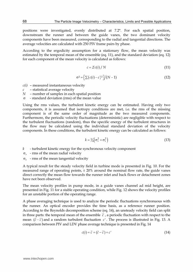
Fig. 12. Mean velocity field in the guide vanes channel for partial load 80%Qn, in pump mode corresponding to an unstable zone on the efficiency curve; planes at 90% and 10% of the guide-vanes channel's height respectively

c c ~

T

t

C

C

c ~

SYNCHRONISATION IMPULSE

' ~ c c 2°

-

Fig. 13. Reynolds decomposition of a velocity signal

Fig. 14. Comparison of phase averaging technique for a PIV and a LDV experiment; data collected in a same spatial location and same operating conditions

www.intechopen.com


71

All the measurements can be superposed in a representative channel due to the good periodicity of the blade-to-blade channels; this periodicity is checked for each measurement point.

The specific turbulent kinetic energy is the summation of the normal stress components. Direct measurement provides two orthogonal components of the velocity field. By assuming turbulence isotropy, the 3 normal stress components have the same order of magnitude, the specific turbulent kinetic energy becomes:

* '2 '23( )

4x zk c c (15)

* '2 '23( )

4x zk c c (16)

Distinction is made between the total kinetic energy (eq. 15) and the turbulent kinetic energy content of the periodic fluctuations (eq. 16). This calculation is a better approach of the specific turbulent kinetic energy because the velocity fluctuation synchronous with the runner position is a deterministic phenomenon and this fluctuation does not concern the specific turbulent energy.

At the runner inlet the difference between the *k and *k calculations is close to 15%, less

important for the design operating point and more important for the off-design operating

points.

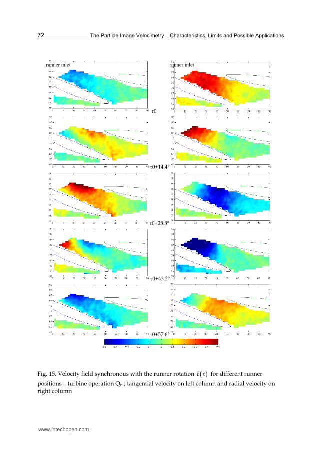
Fig. 15 and Fig. 16 show the unsteady flow propagation in the guide-vane channel for 5

runner positions. This unsteady velocity field distribution shows that the fluctuation of the

velocity components at the runner inlet is the same in all the guide vanes channel.

The blade passage perturbs the flow and therefore leads to a pressure fluctuation at the

runner inlet. This pressure fluctuation induces a velocity fluctuation synchronous with the

runner position. The direction of propagation of this perturbation is not the same for the two

components: in the radial direction for the radial velocity and in tangential direction for the

tangential velocity in the same direction with the runner rotation. The suction side of the

blade produces a suction effect and an increase of the radial velocity. The pressure side of

the blade induces a decrease of the radial velocity and a deviation of the flow direction. The

fluctuating component c c is the same on the two velocity components and corresponds to

30% of the mean velocity.

For the operating conditions corresponding to the unstable region of the efficiency curve,

the same wake phenomenon is observed in the bottom half of the channel, but presents

higher fluctuations than the optimum operation condition – see Fig.17.

In the top half of the channel, the flow is uneven. Analyzing a sequence of synchronous

velocity fields, von Karman vortex structures are detected, propagating in the guide-vanes

channel, as well as flow tendency to re-enter the runner. The von Karman vortex frequency

does not seem to relate to the runner rotation frequency, and the runner wake isn’t present

either. A comparison of the flow topology in different operation conditions is presented in

Fig. 18.

www.intechopen.com


72

0

0+14.4°

0+28.8°

0+43.2°

0+57.6°

Fig. 15. Velocity field synchronous with the runner rotation c for different runner

positions – turbine operation Qn ; tangential velocity on left column and radial velocity on right column

runner inlet runner inlet

www.intechopen.com


73

0( )c

0( 43.2 ) c

0( 21.6 ) c

Fig. 16. Velocity field synchronous with the runner rotation c for nominal flow rate Qn

0 10 20 30 40 50 60 70 80 90 100

60

70

80

90

0 10 20 30 40 50 60 70 80 90 100

60

70

80

90

Fig. 17. Instantaneous velocity fields at 80% of the channel height: optimum flow rate Qn (left) and partial load 0.8Qn (right)

www.intechopen.com


74

0 10 20 30 40 50 60 70 80 90 10055

60

65

70

75

80

85

90

95

0 10 20 30 40 50 60 70 80 90 100

60

70

80

90

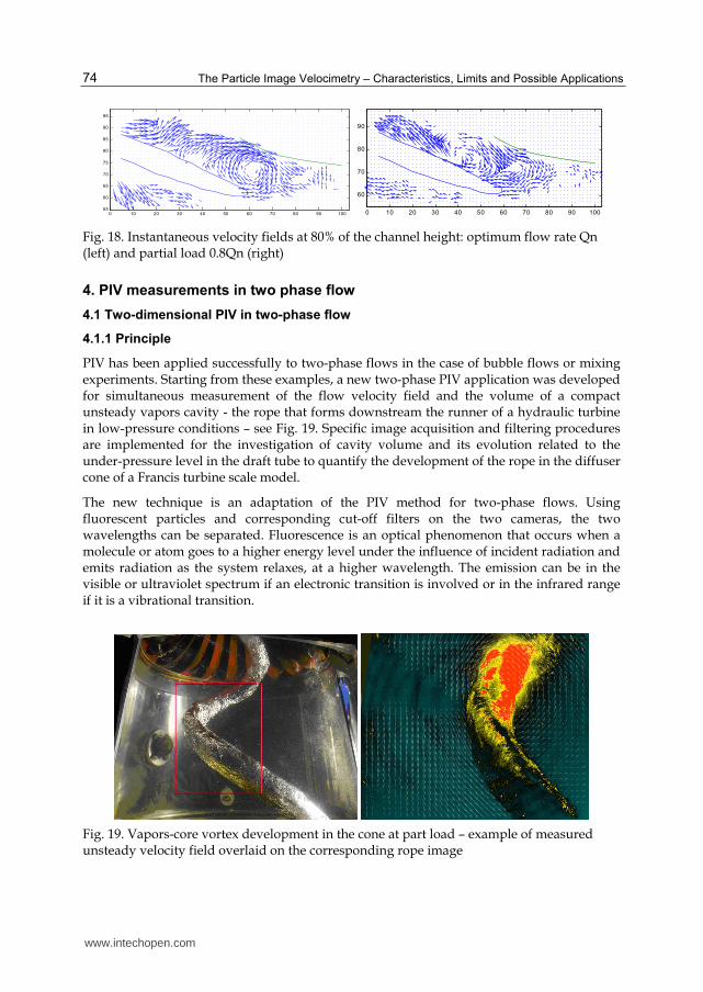
Fig. 18. Instantaneous velocity fields at 80% of the channel height: optimum flow rate Qn (left) and partial load 0.8Qn (right)

4. PIV measurements in two phase flow

4.1 Two-dimensional PIV in two-phase flow

4.1.1 Principle

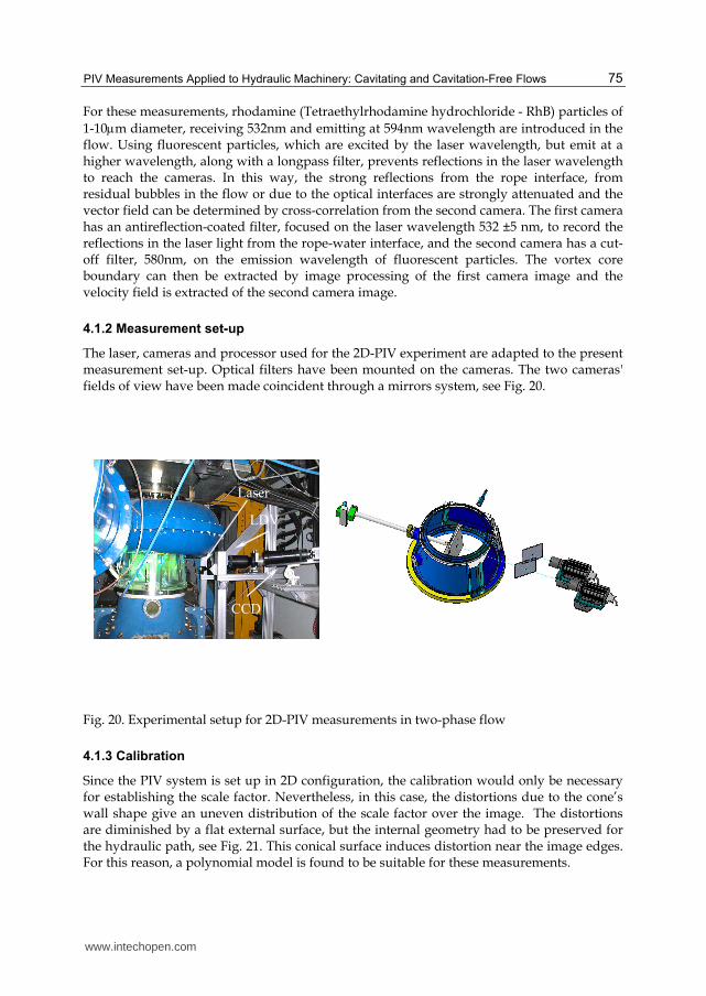
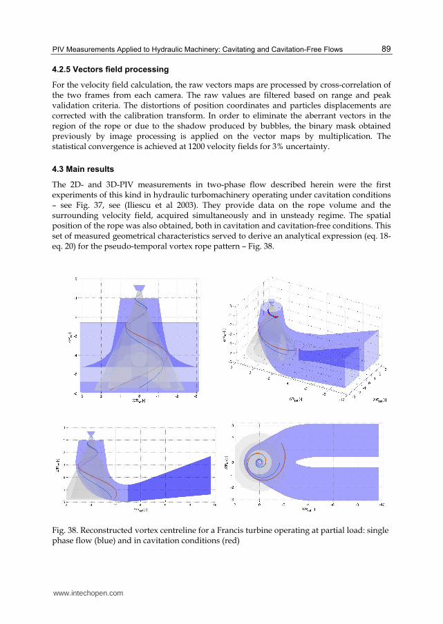
PIV has been applied successfully to two-phase flows in the case of bubble flows or mixing experiments. Starting from these examples, a new two-phase PIV application was developed for simultaneous measurement of the flow velocity field and the volume of a compact unsteady vapors cavity - the rope that forms downstream the runner of a hydraulic turbine in low-pressure conditions – see Fig. 19. Specific image acquisition and filtering procedures are implemented for the investigation of cavity volume and its evolution related to the under-pressure level in the draft tube to quantify the development of the rope in the diffuser cone of a Francis turbine scale model.

The new technique is an adaptation of the PIV method for two-phase flows. Using fluorescent particles and corresponding cut-off filters on the two cameras, the two wavelengths can be separated. Fluorescence is an optical phenomenon that occurs when a molecule or atom goes to a higher energy level under the influence of incident radiation and emits radiation as the system relaxes, at a higher wavelength. The emission can be in the visible or ultraviolet spectrum if an electronic transition is involved or in the infrared range if it is a vibrational transition.

Fig. 19. Vapors-core vortex development in the cone at part load – example of measured unsteady velocity field overlaid on the corresponding rope image

www.intechopen.com


75

For these measurements, rhodamine (Tetraethylrhodamine hydrochloride - RhB) particles of

1-10m diameter, receiving 532nm and emitting at 594nm wavelength are introduced in the flow. Using fluorescent particles, which are excited by the laser wavelength, but emit at a higher wavelength, along with a longpass filter, prevents reflections in the laser wavelength to reach the cameras. In this way, the strong reflections from the rope interface, from residual bubbles in the flow or due to the optical interfaces are strongly attenuated and the vector field can be determined by cross-correlation from the second camera. The first camera has an antireflection-coated filter, focused on the laser wavelength 532 ±5 nm, to record the reflections in the laser light from the rope-water interface, and the second camera has a cut-off filter, 580nm, on the emission wavelength of fluorescent particles. The vortex core boundary can then be extracted by image processing of the first camera image and the velocity field is extracted of the second camera image.

4.1.2 Measurement set-up

The laser, cameras and processor used for the 2D-PIV experiment are adapted to the present measurement set-up. Optical filters have been mounted on the cameras. The two cameras' fields of view have been made coincident through a mirrors system, see Fig. 20.

Laser

LDV

CCD

Fig. 20. Experimental setup for 2D-PIV measurements in two-phase flow

4.1.3 Calibration

Since the PIV system is set up in 2D configuration, the calibration would only be necessary for establishing the scale factor. Nevertheless, in this case, the distortions due to the cone’s wall shape give an uneven distribution of the scale factor over the image. The distortions are diminished by a flat external surface, but the internal geometry had to be preserved for the hydraulic path, see Fig. 21. This conical surface induces distortion near the image edges. For this reason, a polynomial model is found to be suitable for these measurements.

www.intechopen.com


76

a) calibration setup b) calibration target position

Fig. 21. Image calibration setup for 2D-PIV measurements in two-phase flow

4.1.4 Acquisition parameters

The laser energy distribution, camera opening and exposure, seeding density, time interval between pulses and number of acquisitions are adjusted as described in the paragraph 2.

Synchronization

For determining the helical shape of the rope, it is necessary to synchronize the image acquisition with the rope position. The frequency of rope precession is influenced by the σ cavitation level and vapours content in its core. In certain operating conditions it can change over one revolution. Therefore, the triggering system cannot be based on the runner rotation but should detect the rotation frequency of the rope.

The technique to detect the rope precession is based on the measurement of the pressure pulsation generated at the cone wall by the precession of the rope. It has the advantage to work even for cavitation-free conditions when the rope is no longer visible, and, for this reason, it has been selected as trigger for the PIV data acquisition. To characterise the

cavitation level, the - cavitation number is defined:

21

2

a d vP P P

C

(17)

Pa = atmospheric pressure, Pd = water pressure, Pv = water vapour pressure, C = flow velocity and ρ = water density

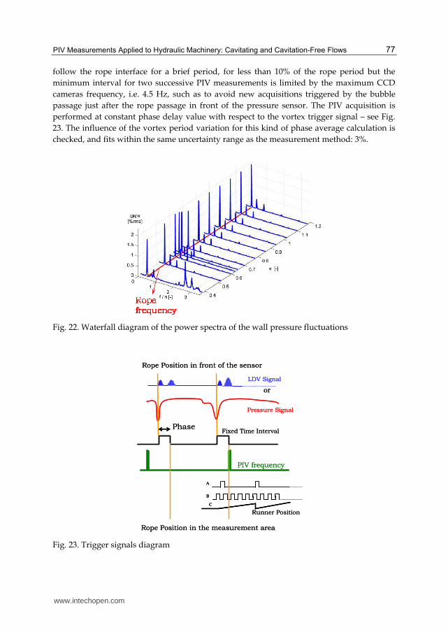
The pressure signals power spectra corresponding to the σ values are represented in the waterfall diagram in Fig. 22. For this operating point, the frequency of the rope precession is decreasing with the σ value.

The correspondence between the wall pressure signal breakdown and the rope spatial

position has been validated through the optical detection of the rope passage using a LDV

probe. By reducing the gain, the photomultiplier of the LDV system delivers a signal each

time the rope boundary or bubbles intersect the LDV measuring volume. Small bubbles

www.intechopen.com


77

follow the rope interface for a brief period, for less than 10% of the rope period but the

minimum interval for two successive PIV measurements is limited by the maximum CCD

cameras frequency, i.e. 4.5 Hz, such as to avoid new acquisitions triggered by the bubble

passage just after the rope passage in front of the pressure sensor. The PIV acquisition is

performed at constant phase delay value with respect to the vortex trigger signal – see Fig.

23. The influence of the vortex period variation for this kind of phase average calculation is

checked, and fits within the same uncertainty range as the measurement method: 3%.

Fig. 22. Waterfall diagram of the power spectra of the wall pressure fluctuations

B

A

C

LDV Signal

Pressure Signal

or

Fixed Time Interval

PIV frequency

Rope Position in the measurement area

Phase

Runner Position

Rope Position in front of the sensor

B

A

C

B

A

C

LDV Signal

Pressure Signal

or

Fixed Time Interval

PIV frequency

Rope Position in the measurement area

Phase

Runner Position

Rope Position in front of the sensor

Fig. 23. Trigger signals diagram

www.intechopen.com


78

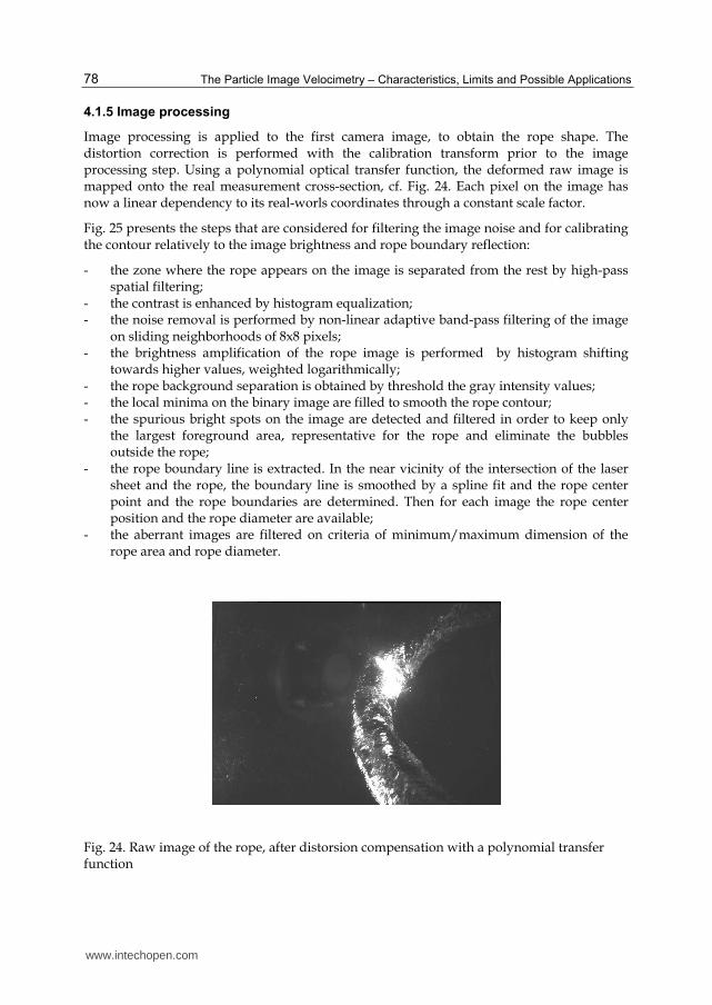
4.1.5 Image processing

Image processing is applied to the first camera image, to obtain the rope shape. The distortion correction is performed with the calibration transform prior to the image processing step. Using a polynomial optical transfer function, the deformed raw image is mapped onto the real measurement cross-section, cf. Fig. 24. Each pixel on the image has now a linear dependency to its real-worls coordinates through a constant scale factor.

Fig. 25 presents the steps that are considered for filtering the image noise and for calibrating the contour relatively to the image brightness and rope boundary reflection:

- the zone where the rope appears on the image is separated from the rest by high-pass spatial filtering;

- the contrast is enhanced by histogram equalization; - the noise removal is performed by non-linear adaptive band-pass filtering of the image

on sliding neighborhoods of 8x8 pixels; - the brightness amplification of the rope image is performed by histogram shifting

towards higher values, weighted logarithmically; - the rope background separation is obtained by threshold the gray intensity values; - the local minima on the binary image are filled to smooth the rope contour; - the spurious bright spots on the image are detected and filtered in order to keep only

the largest foreground area, representative for the rope and eliminate the bubbles outside the rope;

- the rope boundary line is extracted. In the near vicinity of the intersection of the laser sheet and the rope, the boundary line is smoothed by a spline fit and the rope center point and the rope boundaries are determined. Then for each image the rope center position and the rope diameter are available;

- the aberrant images are filtered on criteria of minimum/maximum dimension of the rope area and rope diameter.

Fig. 24. Raw image of the rope, after distorsion compensation with a polynomial transfer function

www.intechopen.com


79

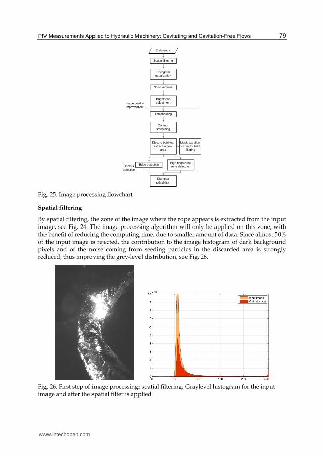
Fig. 25. Image processing flowchart

Spatial filtering

By spatial filtering, the zone of the image where the rope appears is extracted from the input image, see Fig. 24. The image-processing algorithm will only be applied on this zone, with the benefit of reducing the computing time, due to smaller amount of data. Since almost 50% of the input image is rejected, the contribution to the image histogram of dark background pixels and of the noise coming from seeding particles in the discarded area is strongly reduced, thus improving the grey-level distribution, see Fig. 26.

Fig. 26. First step of image processing: spatial filtering. Graylevel histogram for the input image and after the spatial filter is applied

www.intechopen.com


80

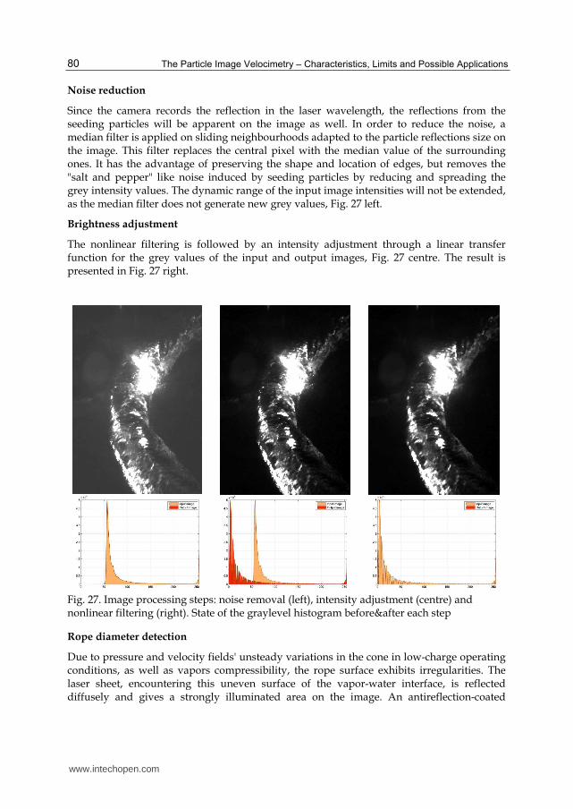
Noise reduction

Since the camera records the reflection in the laser wavelength, the reflections from the seeding particles will be apparent on the image as well. In order to reduce the noise, a median filter is applied on sliding neighbourhoods adapted to the particle reflections size on the image. This filter replaces the central pixel with the median value of the surrounding ones. It has the advantage of preserving the shape and location of edges, but removes the "salt and pepper" like noise induced by seeding particles by reducing and spreading the grey intensity values. The dynamic range of the input image intensities will not be extended, as the median filter does not generate new grey values, Fig. 27 left.

Brightness adjustment

The nonlinear filtering is followed by an intensity adjustment through a linear transfer function for the grey values of the input and output images, Fig. 27 centre. The result is presented in Fig. 27 right.

Fig. 27. Image processing steps: noise removal (left), intensity adjustment (centre) and nonlinear filtering (right). State of the graylevel histogram before&after each step

Rope diameter detection

Due to pressure and velocity fields' unsteady variations in the cone in low-charge operating conditions, as well as vapors compressibility, the rope surface exhibits irregularities. The laser sheet, encountering this uneven surface of the vapor-water interface, is reflected diffusely and gives a strongly illuminated area on the image. An antireflection-coated

www.intechopen.com


81

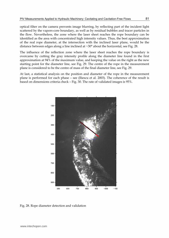
optical filter on the camera prevents image blurring, by reflecting part of the incident light scattered by the vapors-core boundary, as well as by residual bubbles and tracer particles in the flow. Nevertheless, the zone where the laser sheet reaches the rope boundary can be identified as the area with concentrated high intensity values. Thus, the best approximation of the real rope diameter, at the intersection with the inclined laser plane, would be the distance between edges along a line inclined at ~30° about the horizontal, see Fig. 28.

The influence of the reflection zone where the laser sheet reaches the rope boundary is overcame by cutting the gray intensity profile along the diameter line found in the first approximation at 94% of the maximum value, and keeping the value on the right as the new starting point for the diameter line, see Fig. 29. The centre of the rope in the measurement plane is considered to be the centre of mass of the final diameter line, see Fig. 29.

At last, a statistical analysis on the position and diameter of the rope in the measurement plane is performed for each phase – see (Iliescu et al. 2003). The coherence of the result is based on dimensions criteria check – Fig. 30. The rate of validated images is 95%.

Fig. 28. Rope diameter detection and validation

www.intechopen.com


82

Fig. 29. Intensity profile along the approximate diameter

Fig. 30. Lower and upper thresholds for discarding aberrant diameter values

For each image, the intersection of the laser plane with the rope is detected and the values of the rope centre and diameter are transformed into real coordinates, for each validated image. Considering the mean values for each phase, the rope volume is reconstructed by the phase averaging technique.

Binary mask extraction

The binary image also provides a mask for the velocity fields. The pixel values on areas corresponding to each interrogation area for the velocity vector evaluation are averaged and then converted back to binary values. This digital mask thus obtained will be multiplied with the vector values and the zone covered by the rope is eliminated.

Due to the uneven intensity distribution on the zone occupied by the rope, particular image processing steps should be considered for separating the bright rope area from the dark background pixels.

First, the Canny edge-detection method – see (Canny 1986) is applied on the gray level image resulting from the previous steps. This method is based on the computation of the intensity gradient in both horizontal and vertical directions. Applying two threshold values on it gives a binary map of the contours between contrasting portions of the image, Fig. 31a. The boundaries are than thickened by extrapolation, Fig. 31b. Vertical and horizontal nonlinear filters are applied for linking the edges Fig. 31c. After holes filling, Fig. 31d is obtained. Spurious bubbles in the binary image are eliminated and only the largest foreground area is retained, Fig. 31e. Fig. 32f presents the rope contour overlaid on the image.

www.intechopen.com


83

Fig. 31. Image processing steps: edge detection (a), edge dilation (b), edge linking (c), filling connected edges (d), bubble removal from the background (e) and extracted rope contour overlaid on the input graylevel image (f)

4.1.6 Vector field processing

For the velocity field calculation the same processing and validation methods like in

paragraph 4.1.6. are applied, after the extraction of the rope mask from the image – see Fig.

34 and Fig. 35.

www.intechopen.com


84

4.2 Tree-dimensional PIV in two-phase flow

4.2.1 Principle

The new method is an adaptation for two-phase flows of the stereoscopic PIV technique. It

allows obtaining simultaneously the unsteady 3D velocity field and the rope shape. Using

fluorescent particles, which are excited by the laser wavelength, but emit at a higher

wavelength, along with high-pass filters mounted on the cameras, prevents reflections in the

laser wavelength to reach the CCD chip and allows recording the light scattered by

particles. In this way, the strong reflections from the rope boundary, from residual bubbles

in the flow or due to the optical interfaces are eliminated.

Furthermore, using backward illumination in a third wavelength renders a darker rope

shape on a brighter background with a good contrast. It makes the cavity profile sharp

enough for an accurate detection of the rope edges using fewer processing steps for image

enhancement. The constraint consists in adjusting the luminosity level of the background,

such that the bright reflections from seeding particles to be displayed with a good contrast

as well.

4.2.2 Measurement equipment

The laser, cameras and processor used for the 3D-PIV experiment are adapted to the present measurement set-up. Optical filters have been mounted on the cameras’ lenses. For these

measurements, rhodamine (RhB) particles of 1-10m diameter, receiving 532nm and emitting at 594nm wavelength are used as flow-field tracers.

Nominal wavelength

Spectral bandwidth

Luminous intensity

Viewing angle

Operating voltage

Operating current

Power consumption

587 nm 15 nm 280 mcd 120° 10.5 VDC 300 mA 3.2 W

Table 6. LED-array characteristics

Two panels of LEDs, Osram OS-LM01A-Y –Table 6–, placed in front of each camera behind

the cone, insure the backside illumination. Arrays of 22x24 LEDs wired in parallel are

mounted on two plates, and connected to the same power supply system and

synchronization board. A diffusing screen is placed in front of the LED panels.

4.2.3 Calibration & acquisition parameters

The distortions due to the cone wall shape, giving an uneven distribution of the scale factor over the image, are integrated in a calibration model. The distortions are diminished by a flat external surface, but the internal geometry of the hydraulic path had to be preserved, see Fig. 32. This conical surface induces distortion near the image edges. For this reason, a polynomial model, parabolic in Z, is found to be suitable for these measurements.

The laser energy distribution, camera opening and exposure, seeding density, time interval between pulses and number of acquisition are carefully adjusted. The synchronization

www.intechopen.com


85

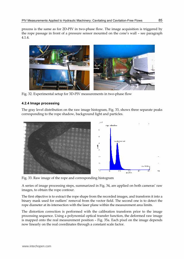
process is the same as for 2D-PIV in two-phase flow. The image acquisition is triggered by the rope passage in front of a pressure sensor mounted on the cone’s wall – see paragraph 4.1.4.

Fig. 32. Experimental setup for 3D-PIV measurements in two-phase flow

4.2.4 Image processing

The gray level distribution on the raw image histogram, Fig. 33, shows three separate peaks corresponding to the rope shadow, background light and particles.

Fig. 33. Raw image of the rope and corresponding histogram

A series of image processing steps, summarized in Fig. 34, are applied on both cameras’ raw images, to obtain the rope contour.

The first objective is to extract the rope shape from the recorded images, and transform it into a binary mask used for outliers’ removal from the vector field. The second one is to detect the rope diameter at its intersection with the laser plane within the measurement area limits.

The distortion correction is performed with the calibration transform prior to the image processing sequence. Using a polynomial optical transfer function, the deformed raw image is mapped onto the real measurement position – Fig. 35a. Each pixel on the image depends now linearly on the real coordinates through a constant scale factor.

www.intechopen.com


86

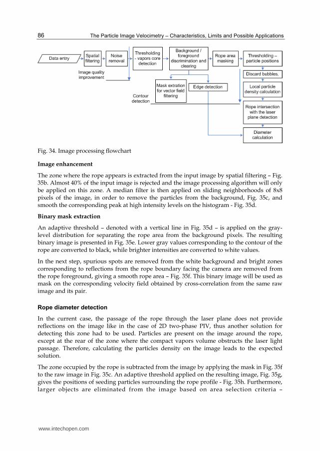
Fig. 34. Image processing flowchart

Image enhancement

The zone where the rope appears is extracted from the input image by spatial filtering – Fig. 35b. Almost 40% of the input image is rejected and the image processing algorithm will only be applied on this zone. A median filter is then applied on sliding neighborhoods of 8x8 pixels of the image, in order to remove the particles from the background, Fig. 35c, and smooth the corresponding peak at high intensity levels on the histogram - Fig. 35d.

Binary mask extraction

An adaptive threshold – denoted with a vertical line in Fig. 35d – is applied on the gray-level distribution for separating the rope area from the background pixels. The resulting binary image is presented in Fig. 35e. Lower gray values corresponding to the contour of the rope are converted to black, while brighter intensities are converted to white values.

In the next step, spurious spots are removed from the white background and bright zones corresponding to reflections from the rope boundary facing the camera are removed from the rope foreground, giving a smooth rope area – Fig. 35f. This binary image will be used as mask on the corresponding velocity field obtained by cross-correlation from the same raw image and its pair.

Rope diameter detection

In the current case, the passage of the rope through the laser plane does not provide reflections on the image like in the case of 2D two-phase PIV, thus another solution for detecting this zone had to be used. Particles are present on the image around the rope, except at the rear of the zone where the compact vapors volume obstructs the laser light passage. Therefore, calculating the particles density on the image leads to the expected solution.

The zone occupied by the rope is subtracted from the image by applying the mask in Fig. 35f to the raw image in Fig. 35c. An adaptive threshold applied on the resulting image, Fig. 35g, gives the positions of seeding particles surrounding the rope profile - Fig. 35h. Furthermore, larger objects are eliminated from the image based on area selection criteria –

www.intechopen.com


87

a) b)

c)

d)

e) f)

g) h)

i)

j)

Fig. 35. Raw image of the rope, after distorsion correction (a); only a section of the active area is used for subsequent image proccessing (b); Image processing stages: noise removal (c) and respective histogram of the filtered image (d); binary image obtained by adaptive thresholding (e); binary mask extraction (f); masking of the rope area (g); detection of particle locations (h); particles selection based on maximum diameter criteria (i); calculation of particle density on horizontal slices (j)

www.intechopen.com


88

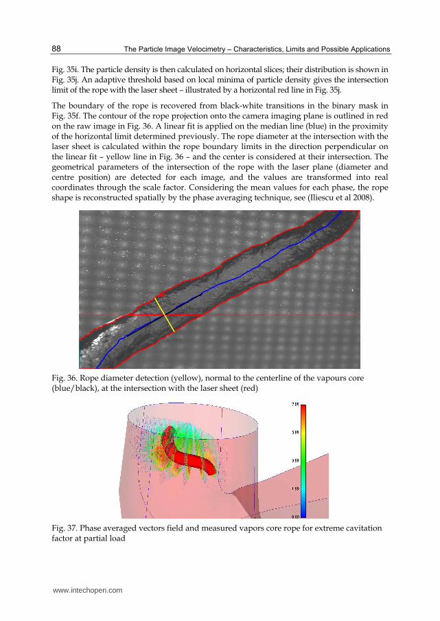
Fig. 35i. The particle density is then calculated on horizontal slices; their distribution is shown in Fig. 35j. An adaptive threshold based on local minima of particle density gives the intersection limit of the rope with the laser sheet – illustrated by a horizontal red line in Fig. 35j.

The boundary of the rope is recovered from black-white transitions in the binary mask in Fig. 35f. The contour of the rope projection onto the camera imaging plane is outlined in red on the raw image in Fig. 36. A linear fit is applied on the median line (blue) in the proximity of the horizontal limit determined previously. The rope diameter at the intersection with the laser sheet is calculated within the rope boundary limits in the direction perpendicular on the linear fit – yellow line in Fig. 36 – and the center is considered at their intersection. The geometrical parameters of the intersection of the rope with the laser plane (diameter and centre position) are detected for each image, and the values are transformed into real coordinates through the scale factor. Considering the mean values for each phase, the rope shape is reconstructed spatially by the phase averaging technique, see (Iliescu et al 2008).

Fig. 36. Rope diameter detection (yellow), normal to the centerline of the vapours core (blue/black), at the intersection with the laser sheet (red)

Fig. 37. Phase averaged vectors field and measured vapors core rope for extreme cavitation factor at partial load

www.intechopen.com


89

4.2.5 Vectors field processing

For the velocity field calculation, the raw vectors maps are processed by cross-correlation of the two frames from each camera. The raw values are filtered based on range and peak validation criteria. The distortions of position coordinates and particles displacements are corrected with the calibration transform. In order to eliminate the aberrant vectors in the region of the rope or due to the shadow produced by bubbles, the binary mask obtained previously by image processing is applied on the vector maps by multiplication. The statistical convergence is achieved at 1200 velocity fields for 3% uncertainty.

4.3 Main results

The 2D- and 3D-PIV measurements in two-phase flow described herein were the first experiments of this kind in hydraulic turbomachinery operating under cavitation conditions – see Fig. 37, see (Iliescu et al 2003). They provide data on the rope volume and the surrounding velocity field, acquired simultaneously and in unsteady regime. The spatial position of the rope was also obtained, both in cavitation and cavitation-free conditions. This set of measured geometrical characteristics served to derive an analytical expression (eq. 18- eq. 20) for the pseudo-temporal vortex rope pattern – Fig. 38.

Fig. 38. Reconstructed vortex centreline for a Francis turbine operating at partial load: single phase flow (blue) and in cavitation conditions (red)

www.intechopen.com


90

r r x i y j z k (17)

( ) 2oor r b (18)

2

2

2

cos

sin

- ( - 1) / tan

o

o

O o

x r b

y r b

z z r b

(19)

The main parameters are given in Table 7, for the investigated operation conditions: cavitation-free flow and maximum vapours core volume.

Cavitation-free vortex Vapors-core vortex

Initial radius ro 0.09 0.15

Initial depth zo -0.615 -1.2

Rate of radial growth b 3.2 4

Cone angle β 17° 25.5°

Table 7. Conical helical vortex model parameters

Fig. 39. Rope centre variations versus the cavitation number

www.intechopen.com


91

Fig. 40. Vortex position variation for two values versus the vortex phase The unsteady analysis of the results the standard deviation of the vortex centre position

representative for the flow stability. The decrease of the standard deviation of the rope

centre with the σ value, Fig. 39, shows that the flow becomes unstable when the volume of

the rope cavity increases. For σ = 0.380, the location of the rope center has an unsteady

spatial variation of ~8% of the local radius of the cone – see Fig. 40. The resonance at this σ

value induces a lost of stability of the rope shape and spatial position are illustrated by

the increase of standard deviation of the vortex center position – twice, from 2% to 4.1% of

the radius.

Fitting a linear equation to the vapors-core vortex radius in the measured positions, added

to the vortex filament model, allows reconstructing the rope volume in the draft tube – see

Fig. 41. In this way, starting with the experimental results, the rope shape and position is

completely parameterized – see (Ciocan et al 2009).

www.intechopen.com


92

Fig. 41. Analytical representation of the vortex rope

In the cone cross-section, the rope center radius is increasing following the phase evolution: the rope goes closer to the wall with the cone depth – see Fig. 42. This evolution is confirmed by the increasing of the wall pressure fluctuation synchronous with the rope rotation, with the cone depth. The standard deviation corresponding to the rope position is quasi-constant for all phases (depth) in the measurement zone.

The procedure to establish the phase average of the rope diameter, already described, is applied for 7 σ values. The rope diameter is represented versus the σ value, as well as the rope center position in the measurement zone. Associated with these values, the standard deviation of the rope diameter and vortex center position is calculated.

The rope diameter is decreasing with the σ value – Fig. 43. The standard deviation of the rope diameter is related to the rope diameter fluctuations and represents the rope volume variations. The physical significance of this calculation is related to the axial pressure waves that produce a volume variation of the rope, due to the local changing of the pressure distribution. The standard deviations are quasi-constant for all σ values at 2.5% of R, except for the value 0.380, where it increases at 4.3% of R. For σ = 0.380 the rope area reported to the local cone section area has a variation between 0.5% and 1.2%.

In fact, for the 0.380 σ value it was pointed out, by hydro-acoustic simulation, that a pressure source located in the inner part of the draft tube elbow induces a forced excitation. This excitation represents the synchronous part of the vortex rope excitation. An eigen frequency of the hydraulic system is also excited at 2.5 of the runner rotation frequency. The plane waves generated by the pressure source, propagating in all the hydraulic circuit, induce consecutively a decreasing and an expansion of the vapors volume of the rope, which explains the increasing of the rope diameter standard deviation for this σ value. Reported to the phase evolution, the rope volume and its standard deviation remain quasi-constant.

www.intechopen.com


93

Fig. 42. Rope diameter variations versus the vortex phase

Fig. 43. Rope diameter variations versus the value

5. Conclusions

The PIV measurement system is a valuable asset for flow dynamics investigations in turbomachines. The PIV measurements, either 2D or 3D, give access to steady values of velocity and turbulent kinetic energy, as well as to their periodic fluctuations. With the help of specific data analysis tools, a wide range of phenomena can be analysed, such as vortex detection and pattern tracking, wake propagation and dissipation, rotor-stator interactions.

www.intechopen.com


94

However, results with the required accuracy are only possible by rigorous developments. The main parameters influencing the measurement accuracy have been identified and their impact on the final result analyzed. A careful choice of the most favorable optical configuration, flawless calibration setup and adequate adjustment of the acquisition parameters are the ingredients of a successful PIV experiment. Furthermore, for investigations in hydraulic turbomachinery the original geometry of the hydraulic profile should be preserved. This requirement adds a degree of complexity due to strong optical deformations and possible local discontinuities in the optical interface, which are difficult to compensate.

Through a specific implementation of the standard PIV technique in two-phase flows, it was possible to evaluate the unsteady flowfield generated by the partial load vortex rope which develops downstream a turbine runner in cavitation conditions, together with the vortex core topology. Specific developments were necessary for the PIV application in cavitation conditions, both in the 2D and the 3D configurations. New image processing tools have been created, allowing simultaneous measurements of the velocity field and related vapours core characteristics. Based on the experimental results, an analytical description of the rope has been determined. The impact of resonance on the rope behaviour was analysed as well.

These measurements represent a valuable database used for theoretical developments as well – see (Susan-Resiga et al. 2006), (Ciocan et al. 2008) the numerical simulations as boundary conditions or validation data – see (Guedes et al. 2002) and (Ciocan et al. 2007).

6. References

Beaulieu S., Deschenes C., Iliescu M., Ciocan G.D., (2009) “Study of the Flow Field Through the Runner of a Propeller Turbine using Stereoscopic PIV“ 3rd IAHR International Meeting of the Workgroup on Cavitation and Dynamic Problems in Hydraulic Machinery and Systems, Brno, Czech Republic, October 14-16

Canny J., (1986) "A Computational Approach to Edge Detection," IEEE Transactions on Pattern Analysis and Machine Intelligence, Vol. PAMI-8, No. 6, pp. 679-698.

Ciocan G.D., (1998) "Contribution à l’analyse des écoulements 3D complexes en turbomachines", PhD Thesis, Institut National Polytechnique de Grenoble

Ciocan G.D., Avellan F., (2004) “Flow Investigations in a Francis Draft Tube: Advanced Experimental Methods” Proceedings of the 3rd Conference of Romanian Hydropower Engineers, Bucarest, Roumanie, Mai 28-29

Ciocan G.D., Iliescu M.S., (2009) “3D PIV Measurements in two phase flow”, 4th International Conference on Energy and Environment, The 1st International Symposium on Green Energy, May, 14-16 – invitated paper

Ciocan G.D., Iliescu M.S. (2008) “3D PIV Measurements in Two Phase Flow and Rope Parametrical Modeling”, 24th IAHR Symposium on Hydraulic Machinery and Systems, Foz do Iguassu, Brazil, October 27-31

Ciocan G.D., Iliescu M.S., Vu T., Nnennemann B., Avellan F., (2007) "Experimental Study and Numerical Simulation of the Flindt Draft Tube Rotating Vortex" - Journal of Fluid Engineering, ISSN: 0098-2202, vol. 129, p. 146-158

Ciocan G.D., Kueny J-L., (2006) "Experimental Analysis of the Rotor-Stator Interaction in a Pump-Turbine", 23rd IAHR Symposium on Hydraulic Machinery and Systems, Yokohama, Japan, October 17 – 21

www.intechopen.com


95

Ciocan G.D., Kueny J-L, Mesquita A.A., (1996) "Steady and unsteady flow pattern between stay and guide vanes in a pump-turbine" - Proceedings of the XVIII International Symposium on Hydraulic Machinery and Cavitation, IAHR, vol. 1, p. 381-390, Valencia, Spain, 16-19 September

Ciocan G.D., Mauri S., Arpe J., Kueny J-L., (2001) "Etude du champ instationnaire de vitesse en sortie de roue de turbine - Etude expérimentale et numérique" - La Houille Blanche no. 2, p. 46-59

Gagnon J.M., Ciocan G.D., Deschênes C., Iliescu M.S., (2008) "Experimental investigation of runner outlet flows in an axial turbine using LDV and stereoscopic PIV", 24th IAHR Symposium on Hydraulic Machinery and Systems, Foz do Iguassu, Brazil, October 27-31

Guedes A., Kueny J-L., Ciocan G.D., Avellan F., (2002) “Unsteady rotor-stator analysis of a hydraulic pump-turbine – CFD and experimental approach” – Proceedings of the XXI International Symposium on Hydraulic Machinery and Cavitation, IAHR, p.767-780, Lausanne, Suisse, 9-12 September

Houde S., Iliescu M.S., Fraser R., Deschênes C., Lemay S., Ciocan G.D., (2011) “Experimental and Numerical Analysis of the Cavitating Part Load Vortex Dynamics of Low-Head Hydraulic Turbines“ Proceedings of ASME-JSME-KSME Joint Fluids Engineering Conference, paper AJK2011-FED, Hamamatsu, Shizuoka, Japan, July 24-29

Iliescu M.S., Ciocan G.D., Avellan F., (2008) "Two Phase PIV Measurements of a Partial Flow Rate Vortex Rope in a Francis Turbine" – Journal of Fluids Engineering, ISSN: 0098-2202, Volume 130, Issue 2, pp. 146-157

Iliescu M.S. (2007) “Large scale hydrodynamic phenomena analysis in turbine draft tubes”, EPFL Thesis n° 3775

Iliescu M.S., Ciocan G.D., Avellan F. (2004): "Experimental Study of the Runner Blade-to-Blade Shear Flow Turbulent Mixing in the Cone of Francis Turbine Scale Model", 22nd IAHR Symposium on Hydraulic Machinery and Systems, Stockholm, Sweden, June 29 – July 2

Iliescu M., Ciocan G.D., Avellan F., (2003) “2 Phase PIV Measurements at the Runner Outlet in a Francis Turbine” The 2003 Joint US ASME-European Fluids Engineering Summer Conference, Honolulu, Hawaii, USA, July 6-10, – Award in the Student Paper Contest

Mesquita A.A., Ciocan G.D., Kueny J-L., (1999) "Experimental Analysis of the Flow between Stay and Guide Vanes of a Pump-Turbine in Pumping Mode" – Journal of the Brazilian Society of Mechanical Sciences and Engineering, ISSN: 1678-5878, vol. 21, no. 4, p. 580-588

Susan-Resiga R., Ciocan G.D., Anton I., Avellan F., (2006) "Analysis of the Swirling Flow Downstream a Francis Turbine Runner" – Journal of Fluids Engineering, vol. 128, p. 177-189

Tridon S., Barre S., Ciocan G.D., Leroy P., Ségoufin C. (2010), “Experimental Investigation of Draft Tube Flow Instability“, Institute of Physics (IoP) Conf. Series: Earth and Environmental Science 12

Tridon S., Barre S., Ciocan G.D., Tomas L., (2010) “Experimental Analysis of the Swirling Flow in a Francis Turbine Draft Tube: Focus on Radial Velocity Component

www.intechopen.com


96

Determination” - European Journal of Mechanics – B/Fluids, ISSN: 0997-7546, vol. 25, Issue 4, pp. 321-335

Tridon S., Ciocan G.D., Barre S., Tomas L., (2008) "3D Time-resolved PIV Measurements in a Francis Draft Tube Cone", 24th IAHR Symposium on Hydraulic Machinery and Systems, Foz do Iguassu, Brazil, October 27-31

www.intechopen.com

The Particle Image Velocimetry - Characteristics, Limits andPossible ApplicationsEdited by PhD. Giovanna Cavazzini

ISBN 978-953-51-0625-8Hard cover, 386 pagesPublisher InTechPublished online 23, May, 2012Published in print edition May, 2012

InTech EuropeUniversity Campus STeP Ri Slavka Krautzeka 83/A 51000 Rijeka, Croatia Phone: +385 (51) 770 447 Fax: +385 (51) 686 166www.intechopen.com

InTech ChinaUnit 405, Office Block, Hotel Equatorial Shanghai No.65, Yan An Road (West), Shanghai, 200040, China

Phone: +86-21-62489820 Fax: +86-21-62489821

The Particle Image Velocimetry is undoubtedly one of the most important technique in Fluid-dynamics since itallows to obtain a direct and instantaneous visualization of the flow field in a non-intrusive way. This innovativetechnique spreads in a wide number of research fields, from aerodynamics to medicine, from biology toturbulence researches, from aerodynamics to combustion processes. The book is aimed at presenting the PIVtechnique and its wide range of possible applications so as to provide a reference for researchers whointended to exploit this innovative technique in their research fields. Several aspects and possible problems inthe analysis of large- and micro-scale turbulent phenomena, two-phase flows and polymer melts, combustionprocesses and turbo-machinery flow fields, internal waves and river/ocean flows were considered.

How to referenceIn order to correctly reference this scholarly work, feel free to copy and paste the following:

Gabriel Dan Ciocan and Monica Sanda Iliescu (2012). PIV Measurements Applied to Hydraulic Machinery:Cavitating and Cavitation-Free Flows, The Particle Image Velocimetry - Characteristics, Limits and PossibleApplications, PhD. Giovanna Cavazzini (Ed.), ISBN: 978-953-51-0625-8, InTech, Available from:http://www.intechopen.com/books/the-particle-image-velocimetry-characteristics-limits-and-possible-applications/piv-measurements-applied-to-hydraulic-machinery-cavitating-and-cavitation-free-flows

© 2012 The Author(s). Licensee IntechOpen. This is an open access articledistributed under the terms of the Creative Commons Attribution 3.0License, which permits unrestricted use, distribution, and reproduction inany medium, provided the original work is properly cited.

http://creativecommons.org/licenses/by/3.0

Date post:	18-Mar-2020
Category:	Documents
Upload:	others
View:	11 times
Download:	1 times

PIV Measurements Applied to Hydraulic Machinery ...cdn.intechopen.com/pdfs/37153/InTech-Piv... ·...

Documents