Placement andPartitioning

ELEC 5402

Pavan Gunupudi

Dept. of Electronics, Carleton University

January 16, 2012

1 / 37

Placement

• Follows synthesis (and verification)

• Placement is done such that:

• No overlap• Chip area is minimal• Sufficient space left for wiring

2 / 37

Partitioning

• Split network into 2 or more parts by cuttinginterconnections.

• Number of interconnections severed should be minimal.

• Partitioning is used in some algorithms to performplacement

3 / 37

Placement

S

R

RS Latch

g2

g1

Output terminalsInput terminals

Q

Q

• Data model of the circuit has:

• Cell (nand)• Port (S, R, Q, Q)• Net (wires)

• Details of cell present in library

4 / 37

Cell-Port-Net

g2

g1Q

Q

n1

n2 n4

n3

S

R

5 / 37

Tripartite Graph

g2

g1n1

n2 n4

n3

S

R Q

Q

6 / 37

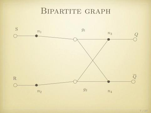
Bipartite graph

g2

g1n1

n2 n4

n3

S

R Q

Q

7 / 37

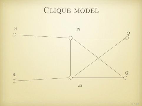
Clique model

g2

g1S

R Q

Q

8 / 37

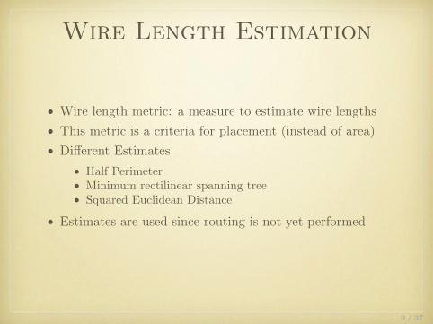
Wire Length Estimation

• Wire length metric: a measure to estimate wire lengths

• This metric is a criteria for placement (instead of area)

• Different Estimates

• Half Perimeter• Minimum rectilinear spanning tree• Squared Euclidean Distance

• Estimates are used since routing is not yet performed

9 / 37

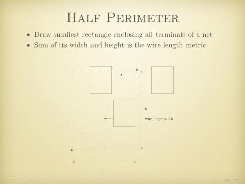
Half Perimeter• Draw smallest rectangle enclosing all terminals of a net

• Sum of its width and height is the wire length metric

l

b

wire length = l+b

10 / 37

Minimum rectilinearspanning tree

• Distance between (x1, y1) and (x2, y2) computed by:• |x1 − x2|+ |y1 − y2| or

• Eucledian distance: ((x1 − x2)2 + (y1 − y2)2)12

11 / 37

Squared Euclidean Distance

• Used for clique models

• Metric:1

2

n∑i=1

n∑j=1

γij [(xi − xj)2 + (yi − yj)2]

• (xi, yj) are the coordinates of the cells, γij is the weightcorresponding to the edges between vertices vi and vj .

• Summation is done over cells, not nets

12 / 37

Standard Cell PlacementClock, power etc

"abut" horizontally

Clock, power etc

All stdcells might not be of same size

13 / 37

Building-Block Placement

• Arbitrary shapes and sizes; general cell layout

14 / 37

Placement Algorithms

• Constructive placement (partitioning methods)

• min-cut partitioning• Clustering

• Iterative improvement

• Perturb-Check-Accept/Repeat

15 / 37

Min-cut Partitioning

• Partition the circuit into two halves such that connectionsbetween the two are minimized

• When nets between two partitions are minimized, thisalgorithm assumes that the “number of long wires crossingfrom one partition to the other are also minimized”

• Repeat partitioning until each partition contains one cell.

16 / 37

Min-cut Partitioning

A B

C D

A B

C D

A B

C D

A B

CD

A

D

C

B

A C

DB

17 / 37

Clustering

• Start with one cell and finds the cells that share many nets

• Form cluster with these cells

• Find another cell that shares many nets with this cluster

• Add this to the cluster

• Repeat until all cells are added to the cluster

18 / 37

Clustering

A B

C D

A B

C D

A B

C D

A B

C D

A A C

A C

B

A C

B D

19 / 37

Iterative Improvement

• Given a certain placement, it is perturbed

• Reevaluate cost function of the placement

• Accept if cost function is better

• Else, optionally discard the perturbed-placement

• Optionally – to avoid local minima and get to global minima

• Generate another perturbation and repeat

• Stop when cost function is good enough

• Similar to general purpose optimization techniques

20 / 37

How To Perturb?

• Main issue is overlap

• Include overlap in cost function along with wire length

• Remove remaining overlap by “pulling apart” cells

• Shift cells after every perturbation

• Computationally intensive for building-block placement• Suitable for standard cells• For standard cells at most half the cells shift

• Store relative positions only

• Free from overlap• Computationally intensive

• Force-directed placement

21 / 37

Force-Directed Placement• Assume cells that share nets feel an “attractive force”

• Calculate centre of gravity of each cell where it experiencesno net force

• Idea: bring all cells towards their centre of gravity

• Centre of gravity (xgi , ygi ) of a cell i is

xgi =

∑j γijxj∑j γij

; ygi =

∑j γijyj∑j γij

• γij is weight of edge (vi, vj) ∈ E• γij = 0 when (vi, vj) /∈ E

• The centre of gravity is calculated for all cells

• Perturbation: move each cell towards its centre of gravity

• If another cell is in place, move it away to an empty spot ortowards its centre of gravity

• Creates chain of moves

22 / 37

Partitioning

• Goal: Split network into 2 or more parts by cuttinginterconnections.

• Number of interconnections severed should be minimal.

• Many algorithms exist to perform partitioning

• One of the famous algorithms is Kernighan and Lin (1970)which we shall study

23 / 37

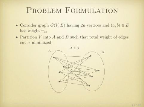
Problem Formulation

• Consider graph G(V,E) having 2n vertices and (a, b) ∈ Ehas weight γab

• Partition V into A and B such that total weight of edgescut is minimized

A BA X B

24 / 37

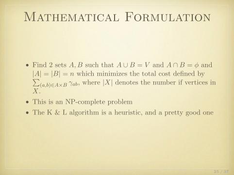
Mathematical Formulation

• Find 2 sets A,B such that A ∪B = V and A ∩B = φ and|A| = |B| = n which minimizes the total cost defined by∑

(a,b)∈A×B γab, where |X| denotes the number if vertices inX.

• This is an NP-complete problem

• The K & L algorithm is a heuristic, and a pretty good one

25 / 37

K & L Algorithm• Choose a random partitioning,

Set of some vertices

Interchange the vertices

A0 B0

X YVA

B

A1 B1

Y X

26 / 37

K & L Algorithm

• If you know exactly which vertices to change, then theproblem can be solved in one iteration

• We don’t know the vertices to swap

• Since the problem is NP-complete

• So we iterate; each iteration is called a pass

• Generally 4 passes are required for the K & L algorithmowing to good heuristics

27 / 37

K & L Pass

• A pass can be represented as:

Am = (Am−1\Xm) ∪ Y m

Bm = (Bm−1\Y m) ∪Xm

• where A\X represents the set where X is removed from A

• Construction of Xm and Y m is based in external andinternal costs of vertices in Am−1 and Bm−1

28 / 37

External Cost

• External cost Ea of a vertex a ∈ Am−1 is

Ea =∑

y∈Bm−1

γay, a ∈ Am−1

• Ea is the measure of pull of vertex a from vertices in Bm−1

• External cost Eb of a vertex b ∈ Bm−1 (measure of pull ofvertex b from vertices in Am−1) is

Eb =∑

x∈Am−1

γbx, b ∈ Bm−1

29 / 37

Internal Cost

• Internal costs, Ia and Ib representing the internal pullswithin Am−1 and Bm−1 can be defined

Ia =∑

x∈Am−1

γax; a ∈ Am−1

Ib =∑

y∈Bm−1

γby; b ∈ Bm−1

30 / 37

Desirability to Move

• DefineDa = Ea − Ia, a ∈ Am−1

Db = Eb − Ib, b ∈ Bm−1

• Da gives an indication of the desirability to move thevertex a

• Db gives an indication of the desirability to move thevertex b

• Define∆ = Da +Db − 2γab, a ∈ Am−1

• ∆ indicates the gain in cut cost due to a swap betweenvertices a and b from Am−1 and Bm−1

31 / 37

K & L Algorithm (steps)1 Compute Da and Db for all a ∈ Am−1, so we get{Da1 , Da2 , . . . , Dan} and {Db1 , Db2 , . . . , Dbn}

2 Find (ai, bi) (edges in the cut) that are unlocked such that

∆i = Dai +Dbi − 2γaibi

is maximal. Lock ai, bi and store ∆i

3 Simulate for other elements in Am−1 and Bm−1 that ai andbi have been interchanged

• For unlocked vertices in Am−1

Dx = Dx + 2γxai− 2γxbi

• For unlocked vertices in Bm−1

Dy = Dy − 2γyai + 2γybi

4 Goto step 3 and repeat until all vertices are locked

32 / 37

K & L Algorithm (steps)

4 Find a k such that G =∑k

i=1 ∆i is maximal• Set of vertices that need to be swapped correspond to the

vertices that were locked in calculating ∆1, . . . ,∆k

5 Form sets Xm and Y m and swap

6 Goto step 1 and iterate as long as overall cut-cost G > 0

• Time complexity of this algorithm is O(n3)

• By sorting elements in Am and Bm, this can be broughtdown to O(n2 log n)

33 / 37

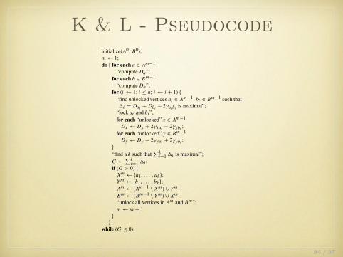
K & L - Pseudocodeinitialize(A0 , B0);

m← 1;

do { for each a ∈ Am−1

“compute Da”;

for each b ∈ Bm−1

“compute Db”;

for (i ← 1; i ≤ n; i ← i + 1) {

“find unlocked vertices ai ∈ Am−1, bi ∈ Bm−1 such that

1i = Dai + Dbi− 2γai bi

is maximal”;

“lock ai and bi”;

for each “unlocked” x ∈ Am−1

Dx ← Dx + 2γxai − 2γxbi;

for each “unlocked” y ∈ Bm−1

Dy ← Dy − 2γyai + 2γybi;

}

“find a k such that∑k

i=1 1i is maximal”;

G←∑k

i=1 1i ;

if (G > 0) {

Xm ← {a1, . . . , ak};

Y m ← {b1, . . . , bk};

Am ← (Am−1 \ Xm ) ∪ Y m ;

Bm← (Bm−1 \ Y m) ∪ Xm ;

“unlock all vertices in Am and Bm”;

m← m + 1

}

}

while (G ≤ 0);

34 / 37

K & L algorithm - Example

5 15 1

1 1 2

1 1

2 1 3

v2

v4 v5

v7v6v3

v8v1

A0 B0

i v2 v3 v6 v7 v1 v4 v5 v8 ∆i

1 5 3 -1 -1 3 3 -1 -3 62 -5 -1 -1 -3 -1 -1 -23 -5 1 -3 3 24 -3 -3 -6

• G =∑k

i=1 ∆i is maximal for k = 1 and 3. Let’s select k = 1• Hence {v2} and {v4} are interchanged

35 / 37

K & L algorithm - Example

5 15 1

1 1 2

1 1

2 1 3 v8v4 v5

v7v6v2 v3

v1

A0 B0

i v3 v4 v6 v7 v1 v2 v5 v8 ∆i

1 -5 -1 -1 -1 -3 -3 -1 -1 -22 5 -3 -3 -7 -5 3 83 -3 -3 -7 -7 -104 1 3 4

• G =∑k

i=1 ∆i is maximal for k = 2• Hence {v3, v4} and {v5, v8} are interchanged

36 / 37

K & L algorithm - Example

5 15 1

1 1 2

1 1

2 1 3 v8v4 v5

v7v6v2 v3

v1

37 / 37