Plan 9: Research Barnegat Bay— - The Official Web Site...

Barnegat Bay—

Year 1

Hard Clams as

Indicators of Suspended

Particulates in Barnegat Bay

Assessment of Stinging Sea

Nettles (Jellyfishes) in

Barnegat Bay

Baseline Characterization of

Zooplankton in Barnegat Bay

Tidal Freshwater &

Salt Marsh Wetland

Studies of Changing

Ecological Function &

Adaptation Strategies

Assessment of Fishes &

Crabs Responses to

Human Alteration

of Barnegat Bay

Baseline Characterization

of Phytoplankton and

Harmful Algal Blooms

Ecological Evaluation of Sedge

Island Marine Conservation

Zone

Barnegat Bay Diatom

Nutrient Inference Model

Plan 9: Research Benthic Invertebrate

Community Monitoring &

Indicator Development for

the Barnegat Bay-Little Egg

Harbor Estuary -

Dr. Olaf Jensen, Rutgers University, Principal Investigator

Heidi Fuchs and Jim Vasslides,

Rutgers University, Co-Investigators

Project Manager:

Tom Belton, Division of Science, Research and

Environmental Health

Thomas Belton, Barnegat Bay Research Coordinator

Dr. Gary Buchanan, Director—Division of Science, Research & Environmental Health

Bob Martin, Commissioner, NJDEP

Chris Christie, Governor

Multi-Trophic Level

Modeling of

Barnegat Bay

June 10, 2013

Year 1 Project Report for “Multi-Trophic Level Modeling of Barnegat Bay”

Olaf Jensen, Heidi Fuchs, and Jim Vasslides

Institute of Marine & Coastal Sciences

Rutgers University

71 Dudley Rd.

New Brunswick, NJ 08901

Objective 1: Develop Conceptual Model of Barnegat Bay Social-Ecological System

Methodology

Fuzzy Logic Cognitive Mapping

To elucidate the ways in which individuals conceptualize the function and operation of the

Barnegat Bay social ecological system we collected a series of Fuzzy Logic Cognitive Maps (FCMs)

from interested stakeholders. FCM are a simplified way of mathematically modeling a complex system

(Ozesmi and Ozesmi 2004), and have been used to represent both individual and group knowledge (Gray

et al. 2011). It has been used to understand processes and decisions in human social systems, the

operation of electronic networks, and in the ecological realm to identify the interactions between social

systems, biotic, and abiotic factors in lakes (Ozesmi 2003, Hobbs et al. 2002) and the summer flounder

fishery (Gray et al. 2011).

FCM are a model of a how a system operates based on key components and the causal

relationships between them. The components can be tangible aspects of the environment (a biotic feature

such as fish or an abiotic factor such as salinity) or an abstract concept such as aesthetic value. The

individual participants identify the components of the system that are important to them, and then link

them with weighted, directional arrows. The weighting can range from -1 to +1, and represents the

amount of influence (positive or negative), that one component has on another.

Data collection

In order to collect FCM from a wide variety of stakeholders with knowledge of the Barnegat Bay

ecosystem we contacted the Barnegat Bay Partnership, an Environmental Protection Agency National

Estuary Program, to obtain a list of their management and science committee members, as well as a list of

public citizens who have expressed long-term interest in the ecosystem. These individuals were then

divided into four groups that were determined a priori; scientists, managers, environmental non-

governmental organizations, and local stakeholders. These groups were selected as they represent the

major categories of stakeholders present in ongoing efforts to manage and improve the bay’s natural

resources. While the map of an individual stakeholder provides information regarding that particular

individual’s conception of the important components and linkages within the system, it can be combined

with other individuals within the group to produce a more robust picture of the group’s understanding of

the system (Ozesmi and Ozesmi 2004). In addition, all of the individual stakeholder maps can be

combined into a community level map depicting the collective understanding of the system.

In accordance with the procedures used in prior FCM’s (Carley and Palmquist 1992, Ozesmi and

Ozesmi 2004, Gray et al. 2011) individuals were interviewed separately, and each interview began with

an overview of the project, a promise of anonymity, and an example of a simple FCM related to an issue

outside of the realm of ecology, namely traffic flow. Interviewee’s were then asked to describe what they

considered to be the key components of the Barnegat Bay social-ecological system, and how those

components relate to one another. They were then asked to score the strength and direction of the

relationship using positive or negative high, medium, or low. The discussion continued until the

interviewee was satisfied that the map as drawn accurately depicted their understanding of the system.

This ranged anywhere from 45 minutes to 180 minutes, with the typical session lasting 90 minutes.

Data Analysis

There are a number of different methods that can be used to analyze the data contained within an

FCM, many of which are based upon graph theory (Harary et al. 1965, Ozesmi and Ozesmi 2004, Kosko

1991). In order to better understand the structure of an individual FCM we translated each map into a

square adjacency matrix, with the variables vi on the vertical axis and vj on the horizontal axis. The

interactions strengths between variables were then scored, with high interactions scored as 0.75, medium

as 0.5, and low as 0.25. A list of all individual variables mentioned throughout the process was compiled

and redundant variables (plurals, different names for the same species, etc.) were eliminated. When two

variables represented opposite directions of the same concept the more prevalent variable was retained

and the other variable was renamed, with the polarity of the interaction reversed, in keeping with accepted

practices (Kim and Lee, 1998).

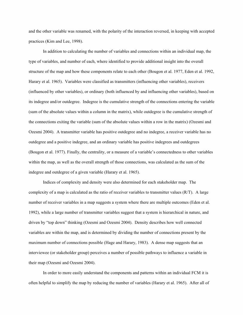
In addition to calculating the number of variables and connections within an individual map, the

type of variables, and number of each, where identified to provide additional insight into the overall

structure of the map and how these components relate to each other (Bougon et al. 1977, Eden et al. 1992,

Harary et al. 1965). Variables were classified as transmitters (influencing other variables), receivers

(influenced by other variables), or ordinary (both influenced by and influencing other variables), based on

its indegree and/or outdegree. Indegree is the cumulative strength of the connections entering the variable

(sum of the absolute values within a column in the matrix), while outdegree is the cumulative strength of

the connections exiting the variable (sum of the absolute values within a row in the matrix) (Ozesmi and

Ozesmi 2004). A transmitter variable has positive outdegree and no indegree, a receiver variable has no

outdegree and a positive indegree, and an ordinary variable has positive indegrees and outdegrees

(Bougon et al. 1977). Finally, the centrality, or a measure of a variable’s connectedness to other variables

within the map, as well as the overall strength of those connections, was calculated as the sum of the

indegree and outdegree of a given variable (Harary et al. 1965).

Indices of complexity and density were also determined for each stakeholder map. The

complexity of a map is calculated as the ratio of receiver variables to transmitter values (R/T). A large

number of receiver variables in a map suggests a system where there are multiple outcomes (Eden et al.

1992), while a large number of transmitter variables suggest that a system is hierarchical in nature, and

driven by “top down” thinking (Ozesmi and Ozesmi 2004). Density describes how well connected

variables are within the map, and is determined by dividing the number of connections present by the

maximum number of connections possible (Hage and Harary, 1983). A dense map suggests that an

interviewee (or stakeholder group) perceives a number of possible pathways to influence a variable in

their map (Ozesmi and Ozesmi 2004).

In order to more easily understand the components and patterns within an individual FCM it is

often helpful to simplify the map by reducing the number of variables (Harary et al. 1965). After all of

the maps were completed we listed the full set of variables and identified those most often mentioned.

We then subjectively combined less frequently mentioned variables into larger categories based on shared

characteristics, a process known as qualitative aggregation. For example, “homes”, “urban development”,

“housing”, and “overdevelopment”, were combined, with a number of other similar variables, into a

category called “development”.

In addition to calculating the variables for each map, maps were combined 1) within stakeholder

groups to produce four group maps and 2) across all individuals to produce a community map. To

combine maps the connection values between two given variables are added, so connections represented

in multiple maps are reinforced (given similar signs) while less common connections are not reinforced,

but are still included in the map (Ozesmi and Ozesmi 2004). In order to compare connection values

across group maps, the summed values are averaged, which provides for equal weighting between all

individual maps.

Results and Discussion

We created fuzzy cognitive maps for 42 individuals from the four targeted stakeholder groups

(Table 1). The number of individuals interviewed from each group is unequal. While the uneven

distribution of interviewees can have an effect on the overall community map, it does not affect the

intragroup comparisons. The importance of the variables in the community map will be slightly weighted

by the scientist’s input, but the important variables in the map were broadly shared across groups. In

addition, a number of managers and NGOs could also have been classified as scientists and individuals in

all categories may be local residents. However, individuals were assigned to a group based on their

interactions with the system rather than their particular background or level of training. For example, a

scientist for an NGO is likely to perceive an issue associated with Barnegat Bay differently than a

state/federal/local manager responsible for a particular suite of resources in the bay, even though the

manager has an advanced science degree also.

The stakeholders identified 349 unique concepts as important to understanding the Barnegat Bay

social – ecological system, which were then aggregated into 84 categories for further analysis. Individual

maps contained an average of 25 concepts, which when aggregated led to an average of approximately 20

categories per map. The average number of categories in an individual map was consistent across all

groups, with the exception of NGOs, who had an average of nearly 30 categories per map (Table 2).

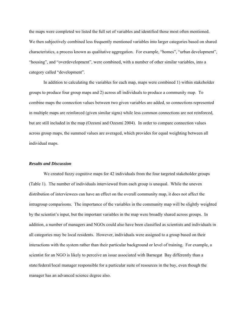
Several of the key structural indices were similar between stakeholder groups (Table 2), though

the importance of particular categories differed both within and between groups (Table 3). There were no

significant differences between the groups in the complexity (df=38, p=0.492) of their maps, though the

environmental NGOs and local people tended to have more receiver variables than the other two groups,

suggesting they think more broadly in terms of potential outcomes. Conversely, the managers and

scientists saw more potential interconnections between their variables as evidenced by their slightly

higher (though not significantly different; df= 38, p=.129) density indices compared to the local people

and environmental NGOs. All stakeholder groups found development to be either the most central, or

second most central, category in the system. In all four maps development had the largest outdegree

score, indicating it exerts its influence throughout the maps, in this case through high interaction strengths

on many other categories. Of note is that while the indegree score for nutrients tended to be higher than

its outdegree score, for both NGOs and Scientists it was still the second largest outdegree score, only

behind that of development.

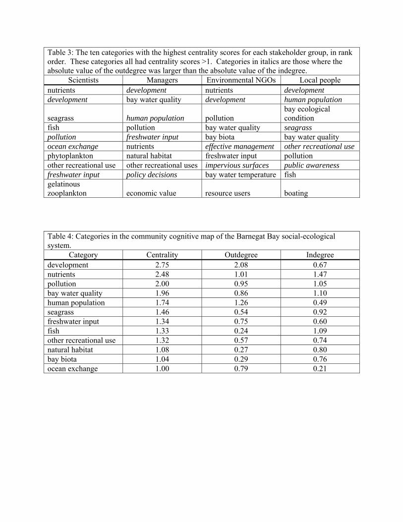
When all of the individual stakeholder maps were aggregated into a community based map

(Figure 1) the density of the map was greater than any of the individual group maps (Table 2), suggesting

that combining knowledge bases led to connections that a single group may have not considered. This

idea of enhanced connections is further supported by the fact that all but one of the 84 categories in the

map is an “ordinary variable”, or those with both incoming and outgoing influences. The categories with

the highest centrality scores, and thus of key importance in the community map, are shown in Table .4 As

expected, development and nutrients are the two most central categories, followed closely by pollution,

bay water quality, and human population. In addition to having the highest centrality scores, these five

categories also have the five highest outdegree scores, suggesting that they are major drivers of the

system.

Table 1: Information on stakeholders who completed fuzzy cognitive maps on the Barnegat Bay social-ecological system

Stakeholder group Maps (N)

People (N)

Occupation/organization/social group

Scientists 19 19 Academic scientists, federal and state agency research scientist

Managers 11 11 Federal, state, county, and local resource managers Environmental NGOs 6 6 Regional, statewide, and local environmental non-

profits Local people 6 6 Baymen, commercial fisherman, local fisherman,

longtime (+40 year) residents

Table 2: Graph indices by stakeholder group. All values, except for number of maps, are mean and standard deviation.

Scientists Managers Environmental

NGOs Local people Community

Maps 19 11 6 6 42 Number of variables (N)

20.6 (4.3) 21.2 (5.3) 29.8 (13.4) 19.3 (3.6) 84

Number of transmitter variables (T)

5.1 (2.7) 4.4 (2.7) 5.8 (3.3) 4.7 (2.5) 0

Number of receivers variables (R)

3.2 (2.8) 2.3 (1.9) 4.5 (2.9) 4.3 (1.8) 1

Number of ordinary variables

12.3 (4.3) 14.5 (4.0) 19.5 (10.8) 10.3 (2.7) 83

Number of connections (C)

38.3 (13.3) 49 (17.8) 64 (40.7) 29.5 (9.3) 1071

C/N 1.9 (0.5) 2.3 (0.6) 2.1 (0.5) 1.5 (0.4) 12.75

Complexity (R/T)

0.7 (0.8) 0.6 (0.5) 0.9 (0.5) 1.1 (0.6)

Density 0.09 (0.03) 0.11 (0.04) 0.08 (0.03) 0.08 (0.02) 0.15

Table 3: The ten categories with the highest centrality scores for each stakeholder group, in rank order. These categories all had centrality scores >1. Categories in italics are those where the absolute value of the outdegree was larger than the absolute value of the indegree.

Scientists Managers Environmental NGOs Local people

nutrients development nutrients development development bay water quality development human population

seagrass human population pollution bay ecological condition

fish pollution bay water quality seagrass pollution freshwater input bay biota bay water quality ocean exchange nutrients effective management other recreational use phytoplankton natural habitat freshwater input pollution other recreational use other recreational uses impervious surfaces public awareness freshwater input policy decisions bay water temperature fish gelatinous zooplankton economic value resource users boating

Table 4: Categories in the community cognitive map of the Barnegat Bay social-ecological system.

Category Centrality Outdegree Indegree

development 2.75 2.08 0.67 nutrients 2.48 1.01 1.47 pollution 2.00 0.95 1.05 bay water quality 1.96 0.86 1.10 human population 1.74 1.26 0.49 seagrass 1.46 0.54 0.92 freshwater input 1.34 0.75 0.60 fish 1.33 0.24 1.09 other recreational use 1.32 0.57 0.74 natural habitat 1.08 0.27 0.80 bay biota 1.04 0.29 0.76 ocean exchange 1.00 0.79 0.21

Figure 1: Community cognitive map of the Barnegat Bay social-ecological system

agriculture

algal blooms

atmospheric deposition

bay biota

bay ecological condition

bay salinity

bay water quality

bay water temperature

benthic biota

benthic infauna

biochemical/physical processes

biodiversity

birdsblue crabs

boating

bulkheading/docks

climate change

commercial fishing

conservation

depth

development

dissolved oxygen

dredging

economic value

ecosystem services

effective management

elected officials

erosion

fishfishing

freshwater input

freshwater quality

freshwater use

gelatinous zooplankton geomorphological processes

government

hard clams

harmful algal blooms

household inputs

human population

impervious surfaces

intangible values

invasive species

larval supply

macroalgae

microbial loop

natural habitat

NGOs

nutrients

ocean exchange

OCNGS

other crustaceans

other groups

other land use

other planktonother recreational use

oysters

phytoplankton

policy decisions

pollution

precipitation

preserved open space

public

public awareness

recreational fishing

regulations

residence time

resource users

runoff

salt marshes

scientists

seagrass

sediment

sewer systems

shellfish

stormwater

tides

tourism

turbidityvehicles

water circulation

wetlands

wind

zooplankton

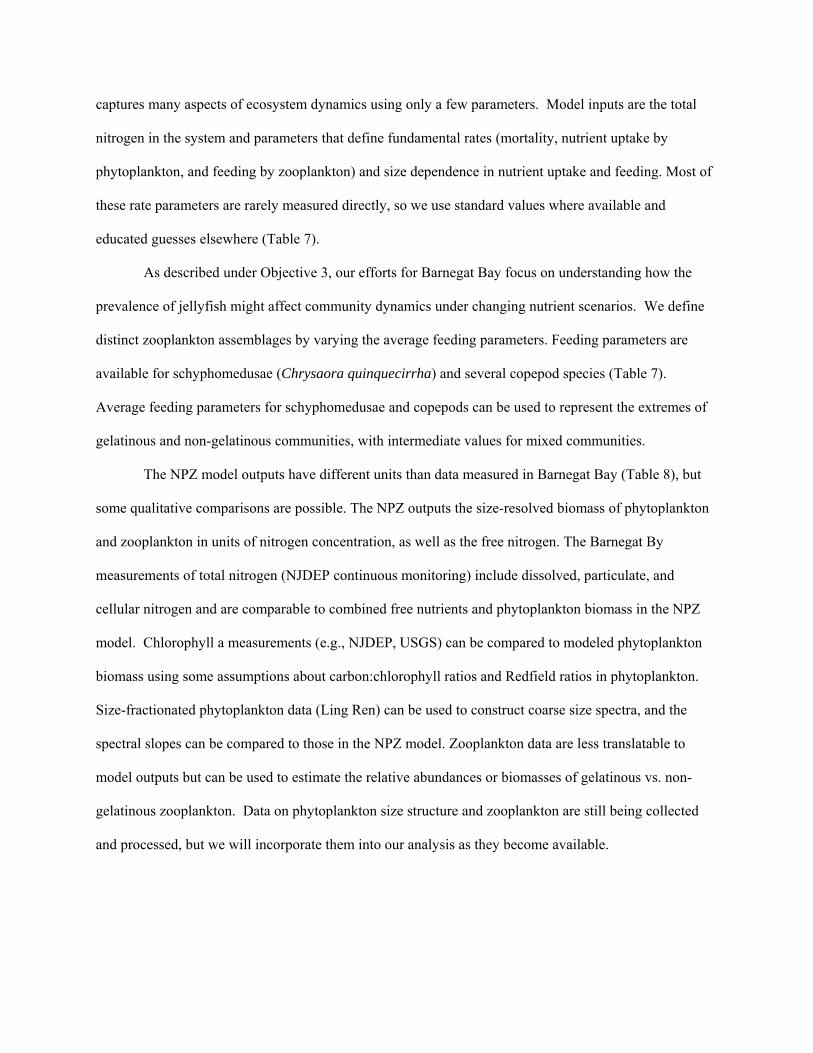
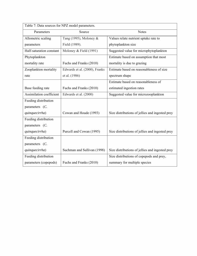
Objective 2 - Gather time series data and model parameters for NPZ and EwE models

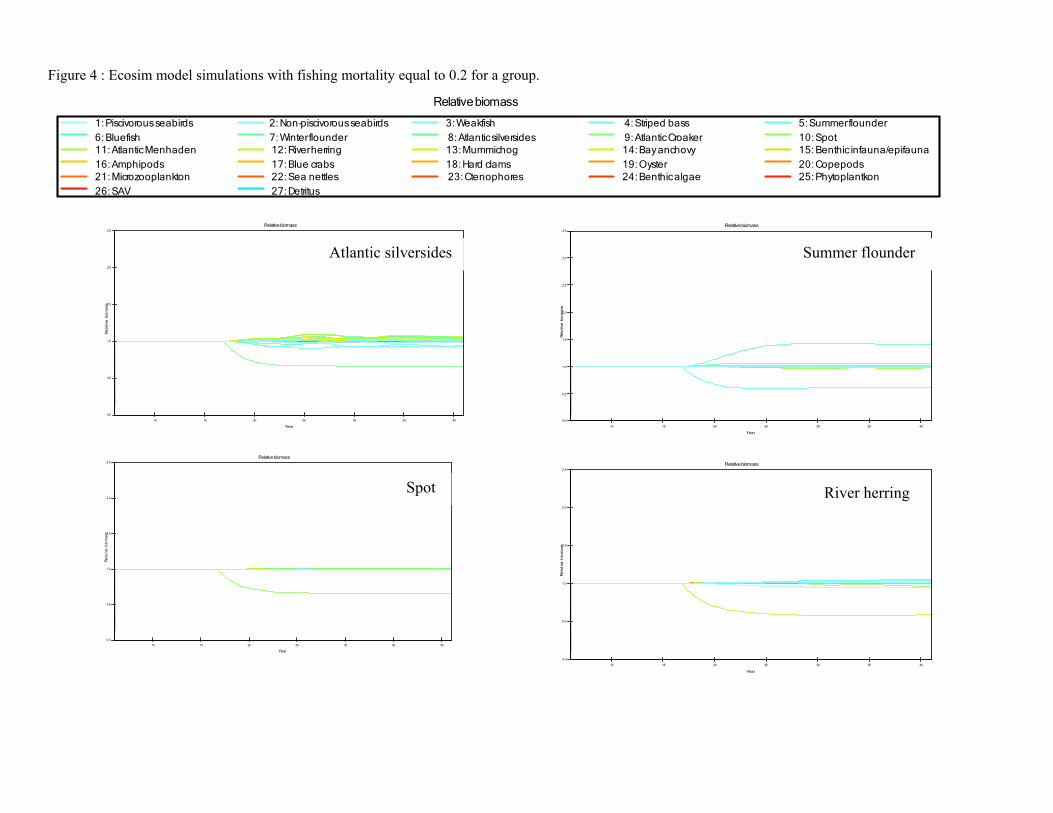
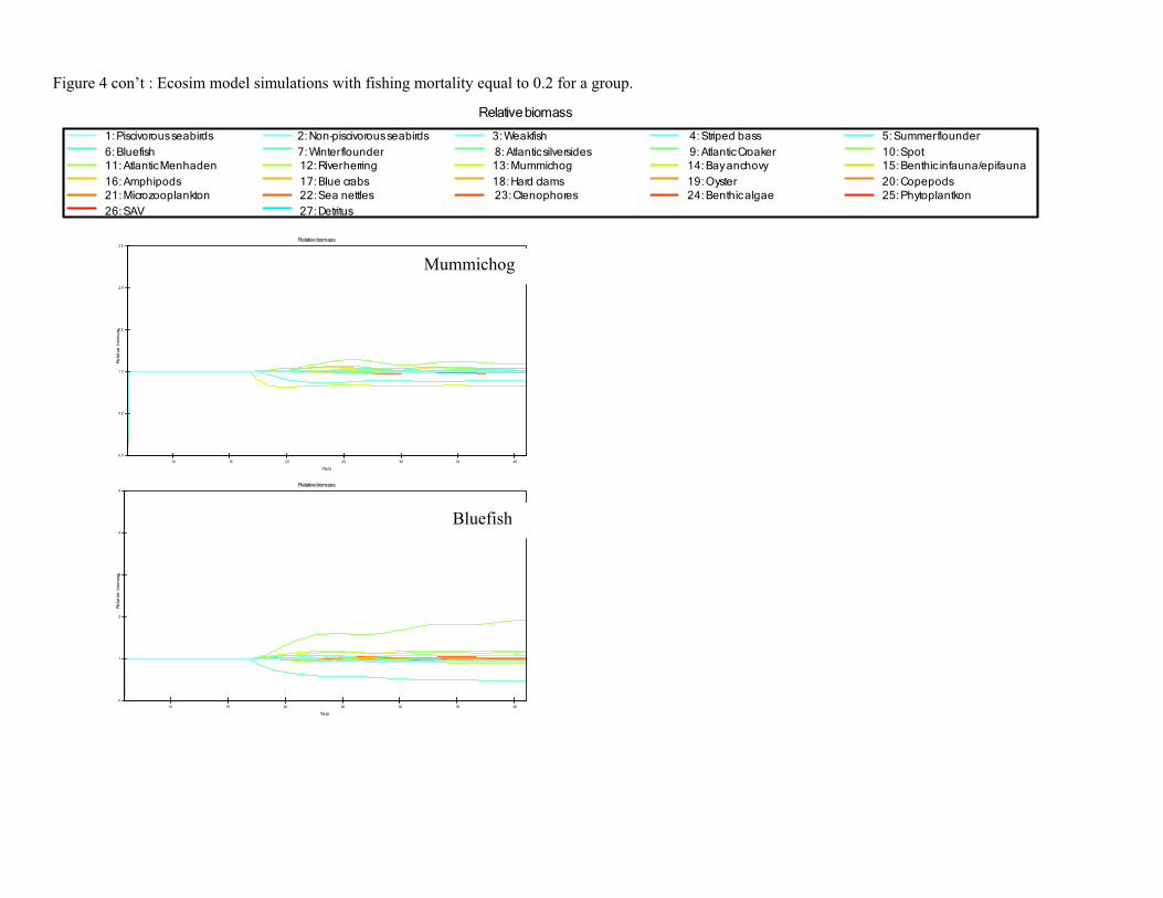
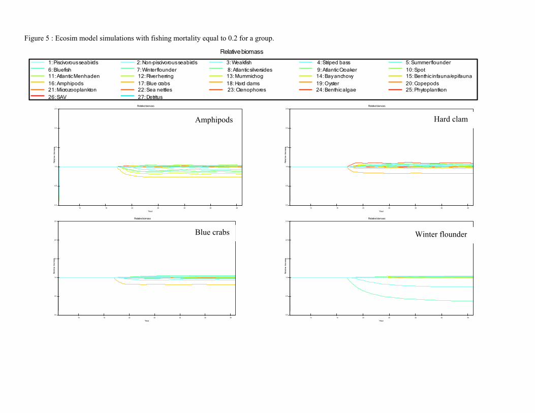
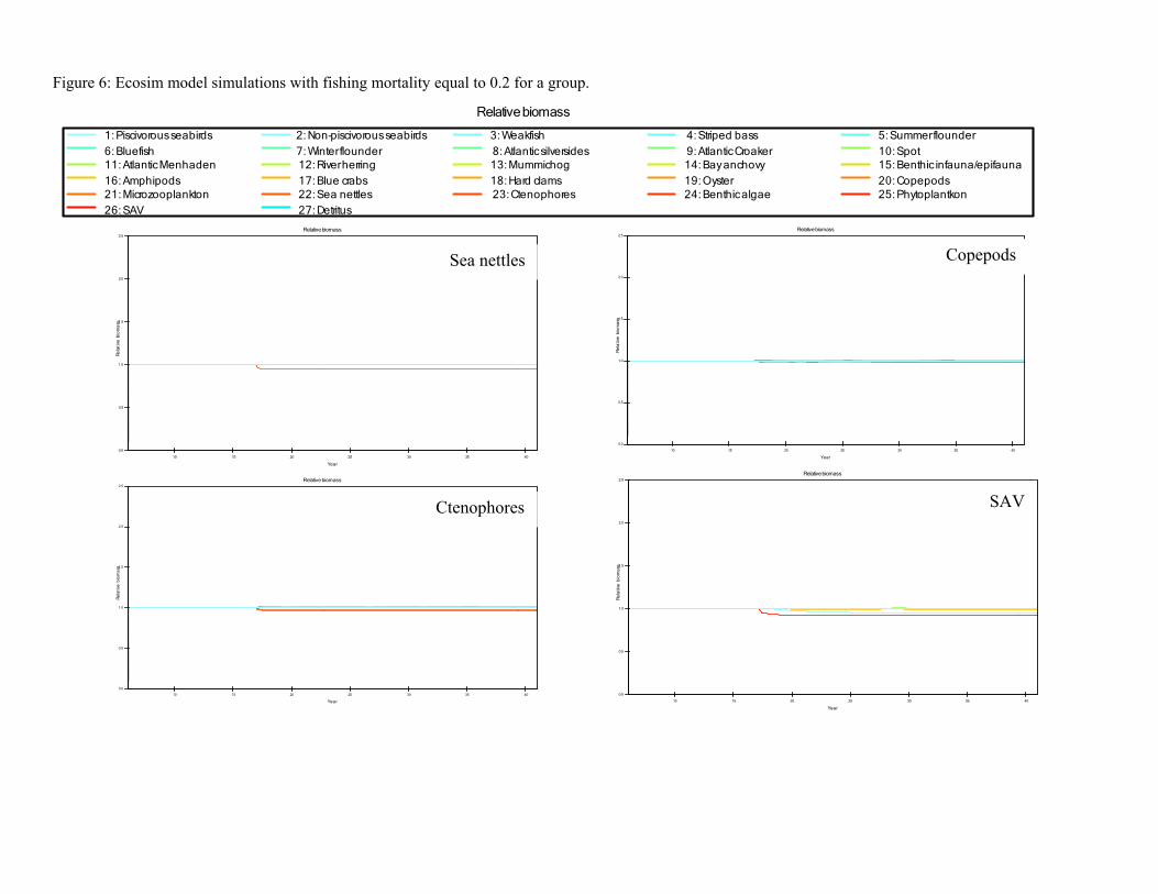
EwE model parameters

Ecopath with Ecosim (EwE) is a software modeling tool used to quantitatively evaluate trophic

interactions within an ecosystem in order to assess options for ecosystem-based management of fisheries.

The first step in the process is to develop a mass-balance model (Ecopath), which requires four groups of

basic input parameters to be entered into the model for each of the species (or groups) of interest: diet

composition, biomass accumulation, net migration, and catch (for fished species). Three of the following

four additional input parameters must also be input: biomass, production/biomass (Z),

consumption/biomass, and ecotrophic efficiency. The model uses the input data along with algorithms

and a routine for matrix inversion to estimate any missing basic parameters so that mass balance is

achieved.

For the purposes of the initial Barnegat Bay model we have set biomass accumulation and net

migration to zero for all of our species groups. This is equivalent to the assumption that biomass of all

species groups was at equilibrium. This is a typical assumption in the absence of information to the

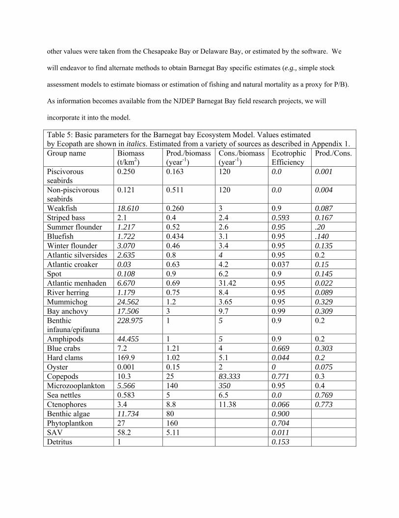
contrary. The biomass, production/biomass, consumption/biomass, and Ecotrophic efficiency initial

estimates for the model can be found in Table 5 below. These parameters were estimated from a variety

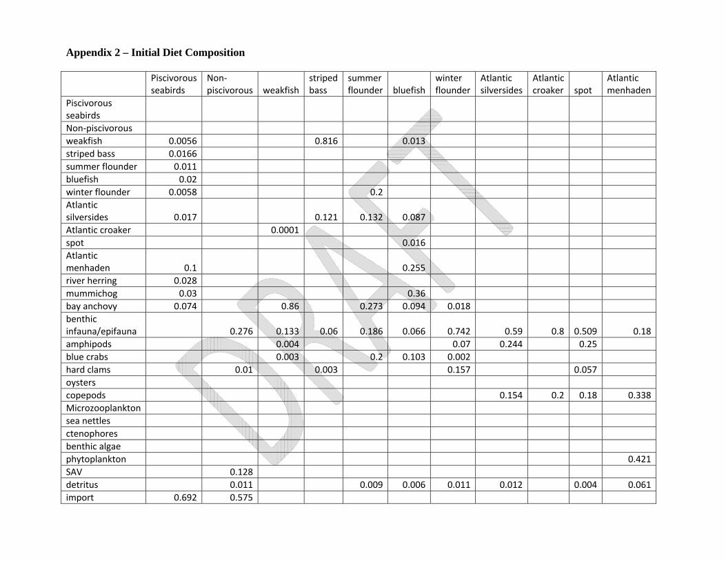
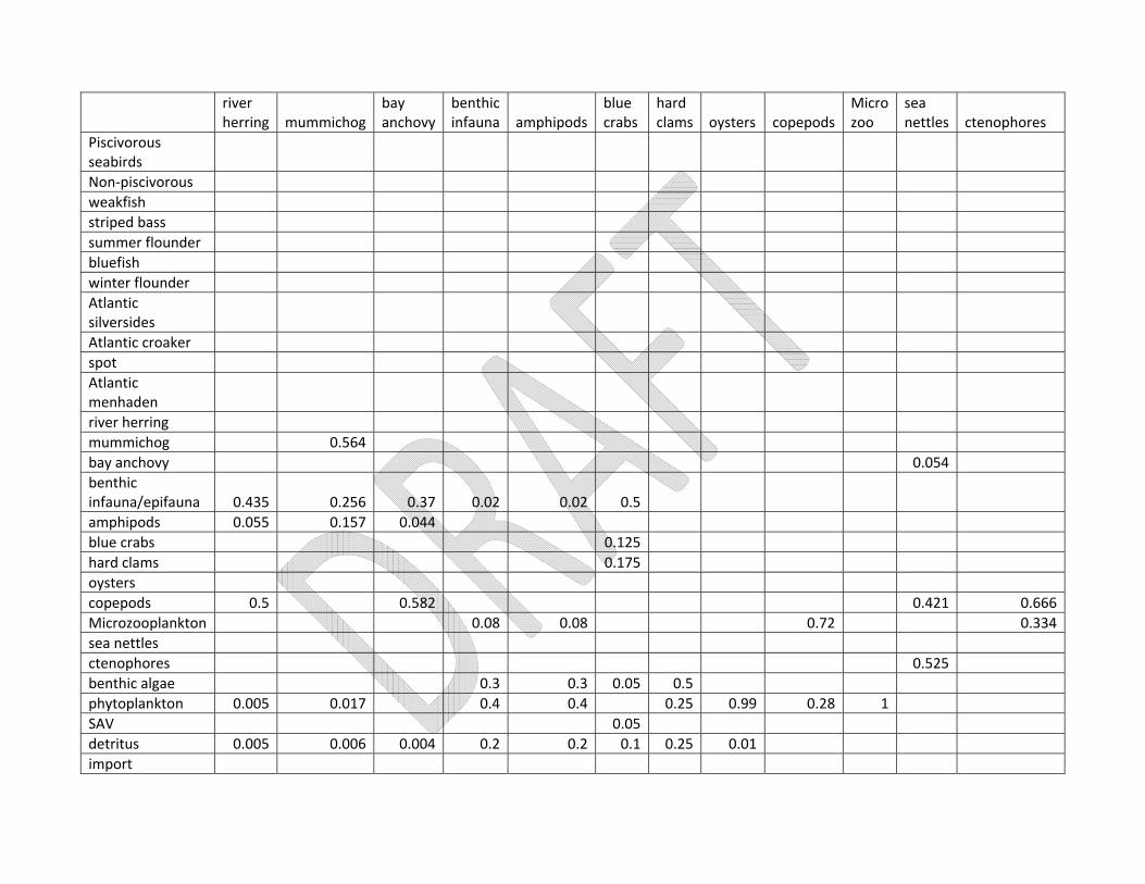
of sources, the details of which can be found in Appendix 1. The initial diet composition matrix can be

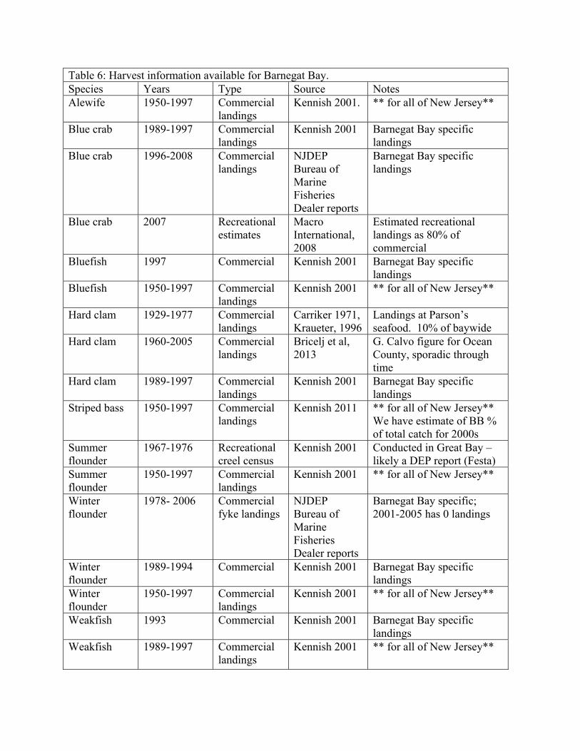
found in Appendix 2, with the source data also listed in Appendix 1. Harvest data for recreationally and

commercially important species can also be incorporated into the EcoPath model as the landings

(t/km2/year) for the year in which the model is initiated. Landings data specific to Barnegat Bay, and

statewide if longer time series are available, are summarized in Table 6.

One of the concerns in the current model is the “lumping” of age/size classes of certain fish and

invertebrate species. While we may have diet data for a number of age/size classes of a given species, we

lack specific information for a number of the other parameters. As identified in Appendix 1, many of the

initial parameters utilized in the model at this time were not developed specifically for Barnegat Bay.

This is particularly true for the biomass estimates, where with the exceptions of SAV and hard clams, the

other values were taken from the Chesapeake Bay or Delaware Bay, or estimated by the software. We

will endeavor to find alternate methods to obtain Barnegat Bay specific estimates (e.g., simple stock

assessment models to estimate biomass or estimation of fishing and natural mortality as a proxy for P/B).

As information becomes available from the NJDEP Barnegat Bay field research projects, we will

incorporate it into the model.

Table 5: Basic parameters for the Barnegat bay Ecosystem Model. Values estimated by Ecopath are shown in italics. Estimated from a variety of sources as described in Appendix 1. Group name Biomass

(t/km2) Prod./biomass (year-1)

Cons./biomass (year-1)

Ecotrophic Efficiency

Prod./Cons.

Piscivorous seabirds

0.250 0.163 120 0.0 0.001

Non-piscivorous seabirds

0.121 0.511 120 0.0 0.004

Weakfish 18.610 0.260 3 0.9 0.087 Striped bass 2.1 0.4 2.4 0.593 0.167 Summer flounder 1.217 0.52 2.6 0.95 .20 Bluefish 1.722 0.434 3.1 0.95 .140 Winter flounder 3.070 0.46 3.4 0.95 0.135 Atlantic silversides 2.635 0.8 4 0.95 0.2 Atlantic croaker 0.03 0.63 4.2 0.037 0.15 Spot 0.108 0.9 6.2 0.9 0.145 Atlantic menhaden 6.670 0.69 31.42 0.95 0.022 River herring 1.179 0.75 8.4 0.95 0.089 Mummichog 24.562 1.2 3.65 0.95 0.329 Bay anchovy 17.506 3 9.7 0.99 0.309 Benthic infauna/epifauna

228.975 1 5 0.9 0.2

Amphipods 44.455 1 5 0.9 0.2 Blue crabs 7.2 1.21 4 0.669 0.303 Hard clams 169.9 1.02 5.1 0.044 0.2 Oyster 0.001 0.15 2 0 0.075 Copepods 10.3 25 83.333 0.771 0.3 Microzooplankton 5.566 140 350 0.95 0.4 Sea nettles 0.583 5 6.5 0.0 0.769 Ctenophores 3.4 8.8 11.38 0.066 0.773 Benthic algae 11.734 80 0.900 Phytoplantkon 27 160 0.704 SAV 58.2 5.11 0.011 Detritus 1 0.153

Table 6: Harvest information available for Barnegat Bay. Species Years Type Source Notes Alewife 1950-1997 Commercial

landings Kennish 2001. ** for all of New Jersey**

Blue crab 1989-1997 Commercial landings

Kennish 2001 Barnegat Bay specific landings

Blue crab 1996-2008 Commercial landings

NJDEP Bureau of Marine Fisheries Dealer reports

Barnegat Bay specific landings

Blue crab 2007 Recreational estimates

Macro International, 2008

Estimated recreational landings as 80% of commercial

Bluefish 1997 Commercial Kennish 2001 Barnegat Bay specific landings

Bluefish 1950-1997 Commercial landings

Kennish 2001 ** for all of New Jersey**

Hard clam 1929-1977 Commercial landings

Carriker 1971, Kraueter, 1996

Landings at Parson’s seafood. 10% of baywide


Bricelj et al, 2013

G. Calvo figure for Ocean County, sporadic through time


Kennish 2001 Barnegat Bay specific landings

Striped bass 1950-1997 Commercial landings

Kennish 2011 ** for all of New Jersey** We have estimate of BB % of total catch for 2000s

Summer flounder

1967-1976 Recreational creel census

Kennish 2001 Conducted in Great Bay – likely a DEP report (Festa)

Summer flounder

1950-1997 Commercial landings


Winter flounder

1978- 2006 Commercial fyke landings

NJDEP Bureau of Marine Fisheries Dealer reports

Barnegat Bay specific; 2001-2005 has 0 landings

Winter flounder

1989-1994 Commercial Kennish 2001 Barnegat Bay specific landings

Winter flounder

1950-1997 Commercial landings


Weakfish 1993 Commercial Kennish 2001 Barnegat Bay specific landings

Weakfish 1989-1997 Commercial landings


EwE time series data

Once the Ecopath model has been balanced the mass-balanced linear equations are then re-

expressed as coupled differential equations so that they can be used by the Ecosim module to simulate

what happens to the species groups over time (Christensen and Walters, 2004). Model runs are compared

with time-series data and the closest fit is chosen to represent the system. Time-series data for model

calibration are thus essential for developing and validating an Ecosim model (Christensen et al. 2009).

Therefore, time-series data depicting trends in relative and absolute biomass, fishing effort by gear type,

fishing and total mortality rates, and catches for as long a period as possible should be viewed as

additional data requirements.

In addition to the commercial landings information in Table 6 there are few other time-series data

available specific to Barnegat Bay. Many other ecosystem models glean data from formal stock

assessments, which utilize similar time series data for single species management plans. While many of

the fish species in our model have been the subject of stock assessment, these are generally coastwide

assessments, and it will therefore be necessary to develop assumptions and correction factors so that these

stock assessments for the larger population can be used in our model.

We have acquired a long-term (1988-2011, except 1991-1995) otter trawl data set from the

Rutgers Marine Field Station that includes 6 regularly sampled sites located in Little Egg Harbor. The

NJDEP has hard clam surveys from 1986/1987 in Barnegat Bay and Little Egg Harbor, 2001 in Little Egg

Harbor, 2011 in Little Egg Harbor, and 2012 in Barnegat Bay. The 1986/1987 and 2001, and 2011 data

are currently available and the 2012 data by 2013.

The final source of time series data will be the other projects currently funded by the NJDEP,

assuming they receive multiple years of funding. We will continue to search for datasets that complement

the ongoing projects in order to lengthen the time series as the model progresses.

Nutrient-Phytoplankton-Zooplankton model

Our working NPZ model is a size-spectrum model detailed in Fuchs and Franks (2010). This model

captures many aspects of ecosystem dynamics using only a few parameters. Model inputs are the total

nitrogen in the system and parameters that define fundamental rates (mortality, nutrient uptake by

phytoplankton, and feeding by zooplankton) and size dependence in nutrient uptake and feeding. Most of

these rate parameters are rarely measured directly, so we use standard values where available and

educated guesses elsewhere (Table 7).

As described under Objective 3, our efforts for Barnegat Bay focus on understanding how the

prevalence of jellyfish might affect community dynamics under changing nutrient scenarios. We define

distinct zooplankton assemblages by varying the average feeding parameters. Feeding parameters are

available for schyphomedusae (Chrysaora quinquecirrha) and several copepod species (Table 7).

Average feeding parameters for schyphomedusae and copepods can be used to represent the extremes of

gelatinous and non-gelatinous communities, with intermediate values for mixed communities.

The NPZ model outputs have different units than data measured in Barnegat Bay (Table 8), but

some qualitative comparisons are possible. The NPZ outputs the size-resolved biomass of phytoplankton

and zooplankton in units of nitrogen concentration, as well as the free nitrogen. The Barnegat By

measurements of total nitrogen (NJDEP continuous monitoring) include dissolved, particulate, and

cellular nitrogen and are comparable to combined free nutrients and phytoplankton biomass in the NPZ

model. Chlorophyll a measurements (e.g., NJDEP, USGS) can be compared to modeled phytoplankton

biomass using some assumptions about carbon:chlorophyll ratios and Redfield ratios in phytoplankton.

Size-fractionated phytoplankton data (Ling Ren) can be used to construct coarse size spectra, and the

spectral slopes can be compared to those in the NPZ model. Zooplankton data are less translatable to

model outputs but can be used to estimate the relative abundances or biomasses of gelatinous vs. non-

gelatinous zooplankton. Data on phytoplankton size structure and zooplankton are still being collected

and processed, but we will incorporate them into our analysis as they become available.

Table 7: Data sources for NPZ model parameters.

Parameters Source Notes

Allometric scaling

parameters

Tang (1995), Moloney &

Field (1989).

Values relate nutrient uptake rate to

phytoplankton size

Half-saturation constant Moloney & Field (1991) Suggested value for microphytoplankton

Phytoplankton

mortality rate Fuchs and Franks (2010)

Estimate based on assumption that most

mortality is due to grazing

Zooplankton mortality

rate

Edwards et al. (2000), Franks

et al. (1986)

Estimate based on reasonableness of size

spectrum shape

Base feeding rate Fuchs and Franks (2010)

Estimate based on reasonableness of

estimated ingestion rates

Assimilation coefficient Edwards et al. (2000) Suggested value for microzooplankton

Feeding distribution

parameters (C.

quinquecirrha) Cowan and Houde (1993) Size distributions of jellies and ingested prey


parameters (C.

quinquecirrha) Purcell and Cowan (1995) Size distributions of jellies and ingested prey


parameters (C.

quinquecirrha) Suchman and Sullivan (1998) Size distributions of jellies and ingested prey


parameters (copepods) Fuchs and Franks (2010)

Size distributions of copepods and prey,

summary for multiple species

Table 8: Data sources from Barnegat Bay-Little Egg Harbor that can be compared to NPZ model outputs.

Includes only data sets that are or will be made publicly available.

Data Years Source Notes

Total Nitrogen 2011-2012

NJDEPa, Monmouth

University, USEPA

14 sites, surface and bottom data, shipboard

measurements, ~4 samples per month

Chlorophyll-a 2011-2012

NJDEPa, Monmouth

University, USEPA

14 sites, surface and bottom data, shipboard

measurements, ~4 samples per month

Chlorophyll-a 2012-2013 NJDEPa, USGS 5 sites, continuous monitoring

Phytoplanktonb 2012-2013 ANSP (Ling Ren) count data, 3 size fractions

Zooplanktonb 2012-2013 Monmouth University

(Ursula Howson)

biovolume CPUE, 2 size fractions, 1-2

samples per month

Gelatinous

Zooplanktonb

2012-2013 Monmouth University

(Ursula Howson)

abundance and size, 1-2 samples per month

Gelatinous

Zooplanktonb

2012-2013 Rutgers University (Ken

Able/Talia Young)

biovolume CPUE, 49 sites, bimonthly

sampling in Spring-early Fall and 1 site

with weekly sampling apublicly available at http://www.state.nj.us/dep/barnegatbay/bbmapviewer.htm banticipated to become available

Objective 3 - Develop initial NPZ and EwE models and evaluate historical predictions of the models

EwE model

The Ecopath model shown in Figure 2 represents a possible configuration of Barnegat Bay for

1980, with the groups arranged by trophic level. There are no surprises in the trophic level of any of the

groups, though striped bass in our system do occupy a slightly higher level than those in the Chesapeake

Bay. The fact that this model output is parsimonious with other models of similar systems lends

additional support to its interpretation. The model is balanced, in that there is sufficient food for the

consumers and enough production to meet consumptive demands.

A sensitivity analysis was undertaken to investigate the influence of each group on the behavior

of the model. A base simulation was run for a period of 50 years, where no changes were made to the

variables (Figure 3, top left panel). As expected, the model remains in equilibrium, and thus a straight

line. An individual parameter perturbation analysis was then conducted by applying an additional

mortality of 0.2 to each group after 15 years to assess the impact of changes in abundance of the modified

group on other groups in the model (Figures 3-6). This step was repeated for each group. A variety of

responses were identified. In some cases the increased mortality on one group (weakfish, striped bass,

menhaden, bay anchovy, benthic infauna) had far ranging effects on most of the other groups in the model

(Figure 3). In other cases the increased mortality lead to small changes to other groups, or larger changes

to only a few groups (Figures 4 and 5). The final response type occurred when the applied mortality was

not large enough to cause any real decrease in the relative biomass of the target group (Figure 6). The

model is most sensitive to the groups identified in Figure 3 and thus additional care should be taken when

reviewing their input values.

When the time series data currently available is incorporated into the model, the fit of the model

prediction to the available data is reasonable (Figure 7, Sum of Squares = 468.6). The model fits most of

the groups well, with changes in relative biomass from the time series data reflected in the model (Figure

8). The model fit to the hard clam data, however, is not as robust as we would like. We are currently

investigating ways to bring the model more in line with the available data.

This EcoSim run includes forcing functions for phytoplankton, benthic algae, and submerged

aquatic vegetation (SAV) in an effort to replicate changes in primary producers over time (Figure 9). The

chlorophyll a (phytoplankton) and benthic algae forcing functions are nearly linear increases over the 32

year of the model run, with a 3x increase from the beginning to the end of the time series. The SAV

function is a nearly linear decrease over the time series. These rates are an estimate of forcing based on

the historic decline in SAV and the anecdotal increase in benthic macroalgae. We are awaiting time

series data on chlorophyll a measurements for the bay, which will be incorporated into the model.

Furthermore, the dynamic linking of the EwE model to the NPZ model will provide additional resolution

to the lower trophic level interactions.

Nutrient-Phytoplankton-Zooplankton Model

Phytoplankton and zooplankton dynamics in Barnegat Bay are expected to reflect variation of

environmental conditions in space and over time. As of the last quarterly report, we intended to use the

NPZ model to investigate whether spatial variation in plankton communities is better explained by

gradients in eutrophication or salinity. After reviewing recent data collected in Barnegat Bay, however,

we concluded that spatial patterns in phytoplankton biomass and size structure are consistent with spatial

variation in nutrient inputs: the northern end of the Bay generally has higher chlorophyll concentrations

and higher abundance of larger phytoplankton than the southern end of the bay (NJDEP continuous

monitoring data , Olsen and Mahoney 2001), as would be expected given the higher nutrient

concentrations in the north. Given that observations can be explained by bottom-up forcing (nutrient

availability), there is little reason to expect that phytoplankton production is strongly affected by salinity.

Moreover, we have found no documentation of salinity dependence in rate parameters for estuarine

plankton. Thus there is little justification for modifying the NPZ model to account for salinity dependence

in rate parameters.

Salinity may have more significant impacts on the composition of zooplankton communities,

particularly the abundance of jellyfish. Although ctenophores (Mnemiopsis leidyi) thrive at a wide range

of salinities (Purcell et al. 2001), there is evidence that scyphomedusae (Chrysaora quinquecirrha) are

most abundant at a salinity of around 15 (Decker et al. 2007). Mean salinities in Barnegat Bay range from

~18ppt in the north to ~25ppt in the south (Moser 1997), although salinity can be <15ppt at the mouth of

the Tom’s River and >30ppt near the inlets (Kennish 2001a). Recent data indicate that these patterns

have remained consistent over time (NJDEP continuous monitoring data). If Barnegat Bay jellyfish

follow similar salinity preferences, then zooplankton communities should be more gelatinous in the north

end of the Bay and more copepod-dominated in the south end of the Bay.

This difference in community composition can be accounted for in our working NPZ model by

changing the feeding parameters. Jellyfish consume a wider size range of prey than crustacean

zooplankton (e.g., copepods), and these different feeding dynamics lead to dichotomous results in the

NPZ model (Fuchs and Franks 2010). The ratio of phytoplankton biomass to free nutrients is higher in a

jelly-dominated model than in a copepod-dominated model (Fig. 10). We calculated a similar ratio (chl a

to nitrate+nitrite concentrations) using data from the continuous monitoring program in Barnegat Bay.

Sites from the north end of the bay have higher phytoplankton-to-free-nutrient ratios than sites in the

south end of the bay, consistent with the hypothesis of a more gelatinous community in the north.

Because zooplankton composition affects community feeding dynamics, the abundance of

jellyfish is relevant to understanding how phytoplankton biomass varies with nutrient inputs. In a

copepod-dominated model a decrease in nutrients always leads to a reduction in phytoplankton biomass,

whereas in a jelly-dominated model, a decrease in nutrients sometimes leads to an unexpected increase in

phytoplankton biomass. This counter-intuitive result may be particularly relevant for management

actions the Tom’s River area of Barnegat Bay, where one potential scenario is a mandated reduction of

nutrient inputs. In year two we will explore nutrient-reduction scenarios in the model to better understand

how these management actions would affect copepod-dominated vs. jelly-dominated plankton

communities.

Figure 2: Barnegat Bay 1980 model. Numbered horizontal lines indicate trophic level.

5

4

3

2

1


Non-piscivorous seabirds

Weakfish

Striped bass

Summer flounder Bluefish

Winter flounderAtlantic silversides Atlantic Croaker Spot

Atlantic Menhaden

River herring

Mummichog

Bay anchovy

Benthic infauna/epifaunaAmphipods

Blue crabs

Hard clams Oyster

Copepods

Microzooplankton

Sea nettles

Ctenophores

Benthic algae Phytoplantkon SAV Detritus

Figure 3 : Ecosim model simulations with additional mortality equal to 0.2 for a group

Relative biomass

1: Piscivorous seabirds 2: Non-piscivorous seabirds 3: Weakfish 4: Striped bass 5: Summer flounder6: Bluefish 7: Winter flounder 8: Atlantic silversides 9: Atlantic Croaker 10: Spot11: Atlantic Menhaden 12: River herring 13: Mummichog 14: Bay anchovy 15: Benthic infauna/epifauna16: Amphipods 17: Blue crabs 18: Hard clams 19: Oyster 20: Copepods21: Microzooplankton 22: Sea nettles 23: Ctenophores 24: Benthic algae 25: Phytoplantkon26: SAV 27: Detritus

Relative biomass

10 15 20 25 30 35 40

Year

0.0

0.5

1.0

1.5

2.0

2.5

Rela

tive

biom

ass

Relative biomass

10 15 20 25 30 35 40

Ye a r

0.0

0.5

1.0

1.5

2.0

2.5

3.0

3.5

Rela

tive

biom

ass

Relative biomass

10 15 20 25 30 35 40

Year

0.0

0.5

1.0

1.5

2.0

2.5

3.0

3.5

Rela

tive

biom

ass

Relative biomass

10 15 20 25 30 35 40

Year

0.0

0.5

1.0

1.5

2.0

2.5

3.0

Rela

tive

bio

mas

s

Base model

Weakfish

Striped bass

Menhaden

Figure 3 con’t : Ecosim model simulations with additional mortality equal to 0.2 for a group.

Relative biomass


Relative biomass

10 15 20 25 30 35 40

Year

0.0

0.5

1.0

1.5

2.0

2.5

Rela

tive

biom

ass

Relative biomass

10 15 20 25 30 35 40

Year

0.0

0.5

1.0

1.5

2.0

2.5

3.0

Rela

tive

biom

ass

Bay anchovy

Benthic infauna

Figure 4 : Ecosim model simulations with fishing mortality equal to 0.2 for a group.

Relative biomass


Relative biomass

10 15 20 25 30 35 40

Year

0.0

0.5

1.0

1.5

2.0

2.5

Rela

tive

bio

mas

s

Relative biomass

10 15 20 25 30 35 40

Year

0.0

0.5

1.0

1.5

2.0

2.5

Rela

tive

biom

ass

Relative biomass

10 15 20 25 30 35 40

Year

0.0

0.5

1.0

1.5

2.0

2.5

3.0

3.5

Rela

tive

biom

ass

Relative biomass

10 15 20 25 30 35 40

Year

0.0

0.5

1.0

1.5

2.0

2.5

Rela

tive

biom

ass

Atlantic silversides

Spot

Summer flounder

River herring

Figure 4 con’t : Ecosim model simulations with fishing mortality equal to 0.2 for a group.

Relative biomass


Relative biomass

10 15 20 25 30 35 40

Year

0.0

0.5

1.0

1.5

2.0

2.5

Rela

tive

biom

ass

Relative biomass

10 15 20 25 30 35 40

Year

0

1

2

3

4

5

Rela

tive

biom

ass

Mummichog

Bluefish

Figure 5 : Ecosim model simulations with fishing mortality equal to 0.2 for a group.

Relative biomass


Relative biomass

10 15 20 25 30 35 40

Year

0.0

0.5

1.0

1.5

2.0

2.5

Rela

tive

biom

ass

Relative biomass

10 15 20 25 30 35 40

Year

0.0

0.5

1.0

1.5

2.0

2.5

Rela

tive

bio

mas

s

Relative biomass

10 15 20 25 30 35 40

Year

0.0

0.5

1.0

1.5

2.0

2.5

Rela

tive

biom

ass

Relative biomass

10 15 20 25 30 35 40

Year

0.0

0.5

1.0

1.5

2.0

2.5

Rela

tive

bio

mas

s

Amphipods

Blue crabs

Hard clam

Winter flounder

Figure 6: Ecosim model simulations with fishing mortality equal to 0.2 for a group.

Relative biomass


Relative biomass

10 15 20 25 30 35 40

Year

0.0

0.5

1.0

1.5

2.0

2.5

Rela

tive

biom

ass

Relative biomass

10 15 20 25 30 35 40

Year

0.0

0.5

1.0

1.5

2.0

2.5

Rela

tive

bio

mas

s

Relative biomass

10 15 20 25 30 35 40

Year

0.0

0.5

1.0

1.5

2.0

2.5

Rela

tive

biom

ass

Relative biomass

10 15 20 25 30 35 40

Year

0.0

0.5

1.0

1.5

2.0

2.5

Rela

tive

biom

ass

Sea nettles

SAV Ctenophores

Copepods

Figure 6: Ecosim model simulations with fishing mortality equal to 0.2 for a group.

Relative biomass


Relative biomass

10 15 20 25 30 35 40

Year

0.0

0.5

1.0

1.5

2.0

2.5

Rela

tive

biom

ass

Relative biomass

10 15 20 25 30 35 40

Year

0.0

0.5

1.0

1.5

2.0

2.5

Rela

tive

biom

ass

Microzooplankton

Phytoplankton

Figure 7:

1: Piscivo6: Bluefis11: Atlan16: Amp21: Micro26: SAV

Model predic

orous seabirdsshntic Menhadenphipodsozooplankton

V

ctions versus t

2: Non-piscivorous s7: Winter flounder12: River herring17: Blue crabs22: Sea nettles27: Detritus

time series da

Relativ

seabirds 3: We8: At13: M18: H23: C

ata for 1980 t

ve biomass

eakfishtlantic silversidesMummichogHard clamsCtenophores

through 2012.

4: Striped bass9: Atlantic Croak14: Bay anchov19: Oyster24: Benthic alga

.

5ker 1vy 1

2ae 2

5: Summer flounder10: Spot15: Benthic infauna/epifau20: Copepods25: Phytoplantkon

una

Figure 8:

EwE mod

Graphs of th

del.

he model fit to

o the currentlyy available timme series dataa for each of tthe groups inn the

Figure 9:

SAV (bot

Forcing funct

ttom).

tions for the EEcoSim modeel run; chloroophyll a (top),, benthic algae (middle), annd

Figure

show th

hypothe

BB06)

BB07-B

high-nu

10: Compari

hat ratio of p

esis of a mor

and a more c

BB14). Note

utrient outlie

ison of Barn

phytoplankto

re gelatinous

copepod-dom

e that units d

er.

negat Bay co

on biomass to

s community

minated com

differ in the t

ontinuous-mo

o free nutrie

y in the north

mmunity in th

two panels.

onitoring dat

ent is consist

h end of the

he south end

The Toms R

ta and NPZ

tent with the

Bay (sites B

d of the Bay

River site (BB

results

BB01-

(sites

B04) is a

Objective 4 - Write and test the program to dynamically link the NPZ and EwE models

This proved to be more technically challenging than anticipated and we have budgeted funds in

Year 2 for a contract programmer at the EwE consortium to complete this task. EwE runs on an annual

time step, which is suitable for capturing the dynamics of longer-lived species such as fish and

corresponds well with the annual reporting of fisheries data. The dynamics of phytoplankton and

zooplankton, however, occur on much finer temporal scales (days to weeks). Meshing these two time

scales will require modification of the EwE model such that the dynamics of some groups can occur on

shorter time scales. We have identified a suitable programmer within the EwE consortium (Jeroen

Steenbeek) and will initiate a contract with him as soon as Year 2 funds are available.

Objective 5 and 6- Develop and run quantitative change scenarios

During the conceptual model development interviews we asked individuals to tell us what

variables in their cognitive maps they would increase or decrease the values of in order to effect

“positive” change on the bay ecosystem. The responses included changes to both social and ecological

components of the system, the impacts of some of which we can model in the EwE, and to a lesser extent

in the NPZ, models.

Scenario 1 – Oyster Creek Nuclear Generating Station (OCNGS) closure

As America’s oldest continuously operating nuclear plant, the facility uses a once-through

cooling water system, where water is drawn from Forked River, used to cool the plant, and is then

returned to Oyster Creek to flow into the bay. The impingement and entrainment of fish, crab, and hard

clam larvae, as well as other zooplankters, is well documented. OCNGS functions as a de facto fishery,

and the removal of biomass from the system is accounted for through catch data used in the EwE model.

As part of the Governor’s 10-point Plan, the Oyster Creek Nuclear Generating Station (OCNGS) will

cease power generation by 2020. To model this scenario we reduced the “catch” of the plant from the

“catch” at full operating capacity to 4% of the full operating capacity beginning in 2020, based on the

percent reduction in intake water that is planned. The time series data was amended so that the 2011

values for the forced catches and effort series were used for 2012-2030, with the previously noted

exception of OCNGS effort. The chlorophyll a, benthic macroalage, and SAV forcing was set to the 2011

level for the remainder of the simulation. Under those model parameters the relative biomass of the fish

and other secondary consumers remains stable, while the primary consumers show a slight increase

(Figure 11). If the forced catches and effort data for 2012-2030 are the average of the 1980-2011 data,

the results are similar.

The closure of the plant is not expected to have an effect on NPZ model parameters, which are

independent of temperature. Temperature dependence is rarely included in NPZ models and would be a

major modification, therefore this scenario will be run in EwE only.

Scenario 2 – Changes to blue crab management strategy

Blue crabs are Barnegat Bay’s largest commercial fishery, and are currently managed based on a

mix of sex and size limits and seasonal closures (NJAC7E:25 and 25A). We modeled the effects of

increasing the commercial dredge harvest to 92 metric tons. (twice the 1996-2006 average of 46 MT.) and

of decreasing the commercial dredge harvest to 23 MT (one-half the ten year average) from 2012 to 2030,

while keeping the commercial pot fishery and recreation fishery at the 1996-2006 average. Doubling or

halving the commercial dredge had little effect on crab biomass (Figure 12). We also modeled the effects

of doubling the commercial pot fishery over the 1996-2006 average of 218 MT to 436 MT and of halving

it to 109 MT. Reducing or increasing the landings in the commercial pot fishery had little effect on crab

biomass (Figure 13). The results are not unexpected given that the largest landings modeled (436 MT) is

only 4% of the available modeled biomass (38MT/km2).

Scenario 3 – Changes to hard clam management strategy

Hard clams were historically one of the most important commercial fisheries in the Bay, but

landings have declined dramatically over the past several decades. We will model the effects of limiting

the commercial harvest to 25,000 lbs. (approximate 2005 landings) and of closing the fishery entirely for

a period of ten years. Because of the trouble we are having with fitting the model to the existing hard

clam data we have not modeled this scenario at this time. Once the model fit for hard clams has been

improved we will run this analysis.

Scenario 4 – Nutrient input reduction

The Barnegat Bay has been described as a moderately eutrophic estuarine system, and the focus

of recent legislation (NJ Fertilizer Act, P.L. 2010 Chapter 112; NJ Soil Restoration Act, P.L. 2010

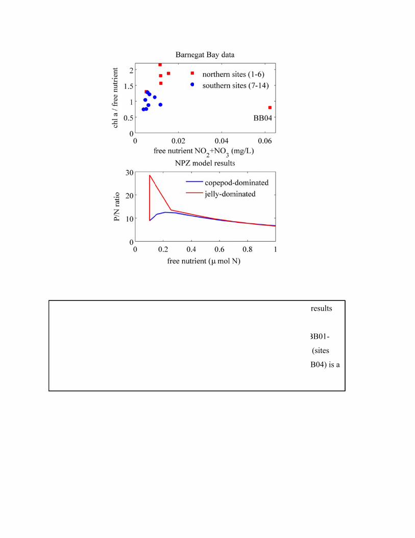
Chapter 113) and restoration efforts (NJ Stormwater Act, P.L. 2010 Chapter 114; Clean Water Act

Section 319 projects) in New Jersey has been to reduce the amount of nitrogen being delivered into the

system. As no target reductions have been set at this time, we propose to model the effects of reducing

nitrogen inputs by 5% and 15%. The effects of these reductions on phytoplankton and zooplankton

biomass and/or production in the NPZ model will then be translated to changes in the EwE model for the

same groups. Furthermore, we will adjust the P/B ratio for the seagrass group in the EwE model based on

the relationship found in Tomasko et al. (1996) on seagrass productivity and nitrogen loading. Dynamic

linking of the two models for the nutrient change scenario will be accomplished in Year 2, after the code

linking the NPZ and EwE models is written.

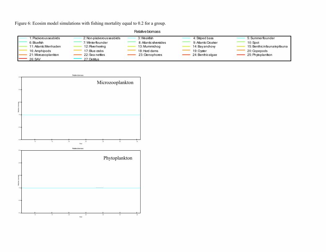
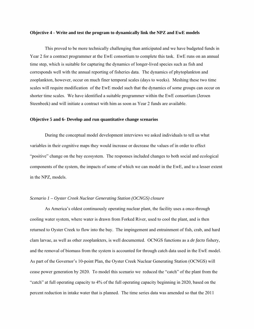
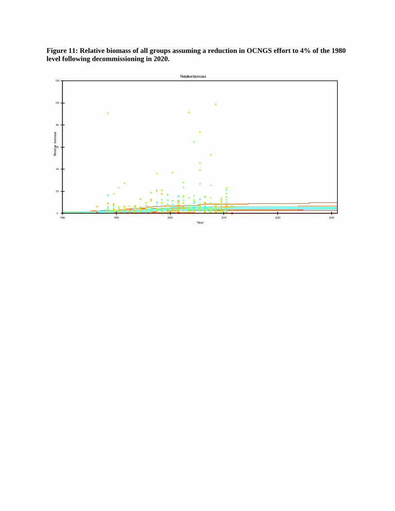
Figure 11: Relative biomass of all groups assuming a reduction in OCNGS effort to 4% of the 1980 level following decommissioning in 2020.

Relative biomass

1980 1990 2000 2010 2020 2030

Year

0

20

40

60

80

100

120

Rela

tive

biom

ass

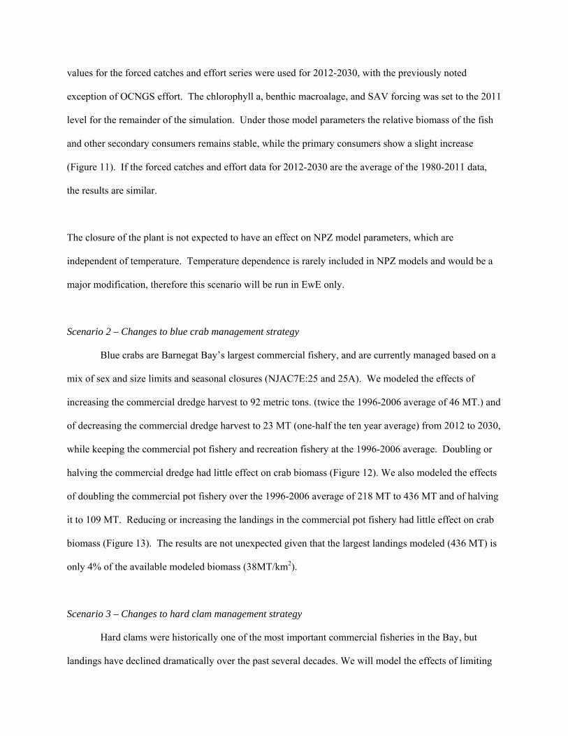
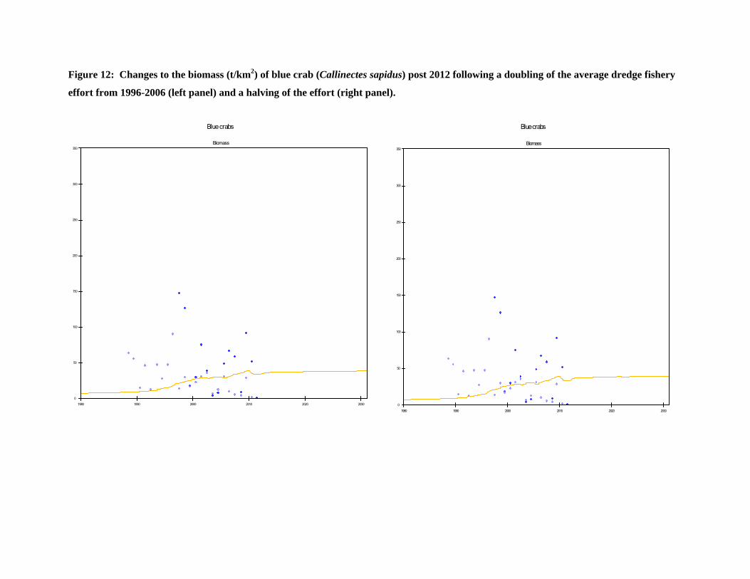
Figure 12: Changes to the biomass (t/km2) of blue crab (Callinectes sapidus) post 2012 following a doubling of the average dredge fishery

effort from 1996-2006 (left panel) and a halving of the effort (right panel).

Blue crabs

Biomass

1980 1990 2000 2010 2020 2030

0

50

100

150

200

250

300

350

Blue crabs

Biomass

1980 1990 2000 2010 2020 2030

0

50

100

150

200

250

300

350

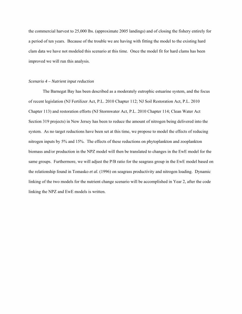
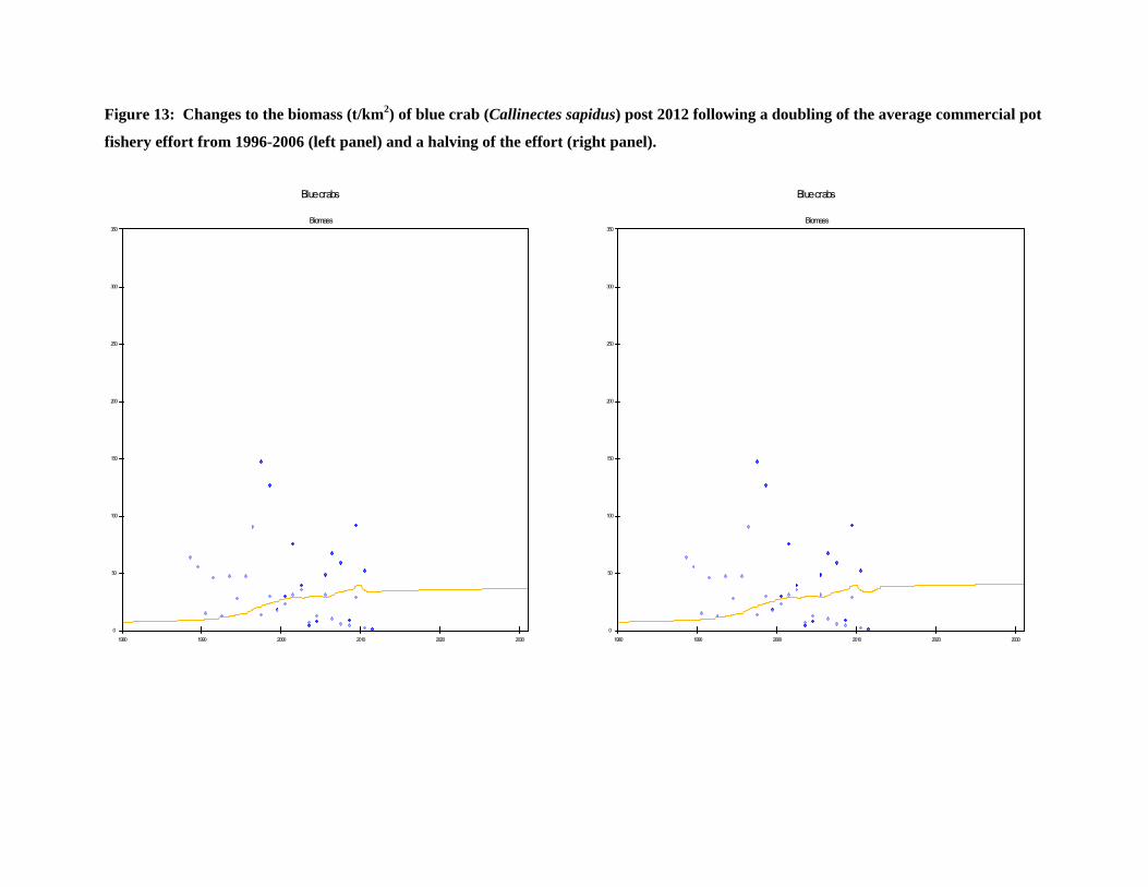
Figure 13: Changes to the biomass (t/km2) of blue crab (Callinectes sapidus) post 2012 following a doubling of the average commercial pot

fishery effort from 1996-2006 (left panel) and a halving of the effort (right panel).

Blue crabs

Biomass

1980 1990 2000 2010 2020 2030

0

50

100

150

200

250

300

350

Blue crabs

Biomass

1980 1990 2000 2010 2020 2030

0

50

100

150

200

250

300

350

References Anderson, D.R., 1975. Population ecology of the mallard, V: Temporal and geographic estimates of survival, recovery, and harvest rates. U.S. Fish and Wildl. Serv. Resour. Publ., 25:110. ASMFC. 2003 Atlantic striped bass advisory report. ASMFC Striped Bass Technical Committee Report 2003-03, Atlantic States Marine Fisheries Commission, Washington, D.C. Baird, D. and Ulanowicz, R.E., 1989. The seasonal dynamics of the Chesapeake Bay ecosystem. Ecological Monographs, 59:329-364. Bougon, M., Weick, K., Binkhorst, D., 1977. Cognition in organizations: an analysis of the Utrecht Jazz Orchestra. Admin. Sci. Quart. 22, 606–639. Bricelj, V. M., J.N. Kraeuter, and G. Flimin. 2013. Status and Trends of Hard Clam, Mercenaria mercenaria, Shellfish Populations in Barnegat Bay, New Jersey. Barnegat Bay Partnership Technical Report. Toms River, Barnegat Bay Partnership: 143. Christensen, V. and Walters, C.J., 2004. Ecopath with Ecosim: methods, capabilities and limitations. Ecol. Model., 172:109-139. Christensen, Villy, and Alasdair Beattie, Claire Buchanan, Hongguang Ma, Steven J. D. Martell, Robert J. Latour, Dave Preikshot, Madeline B. Sigrist, James H. Uphoff, Carl J. Walters, Robert J. Wood, and Howard Townsend. 2009. Fisheries Ecosystem Model of the Chesapeake Bay: Methodology, Parameterization, and Model Explanation. U.S. Dep. Commerce, NOAA Tech. Memo. NMFS-F/SPO-106, 146 p. Christensen, V., Walters, C.J. and Pauly, D., 2005. Ecopath with Ecosim: a User's Guide, November 2005 Edition, Fisheries Centre, University of British Columbia, Vancouver, Canada. Carley, K., Palmquist, M., 1992. Extracting, representing, and analyzing mental models. Social Forces 70, 601–636. Cowan, J. H. J. and E. D. Houde. 1993. Relative predation potentials of scyphomedusae, Ctenophores and planktivorous fish on ichthyoplankton in Chesapeake Bay. Marine Ecology Progress Series 95: 55-65. Eden, C., Ackerman, F., Cropper, S., 1992. The analysis of cause maps. J. Manage. Stud. 29, 309–323 Edwards, C. A., T. M. Powell, and H. P. Batchelder. 2000. The stability of an NPZ model subject to realistic levels of vertical mixing. Journal of Marine Research 58: 37-60. Franks, P. J. S., J. S. Wroblewski, and G. R. Flierl. 1986. Behavior of a simple plankton model With food-level acclimation by herbivores. Marine Biology 91: 121-129. Frisk, M.G., T.J. Miller, R.J. Latour, and S. Martell. 2006. An ecosystem model of Delaware Bay.

Froese, R. and Pauly, D., 2004. FishBase, World Wide Web electronic publication, www.fishbase.org,version (03/2013). Fuchs HL, Franks PJS. 2010. Plankton community properties determined by nutrients and size selective feeding. Marine Ecology Progress Series, 413: 1-15. Gray, S., A. Chan, D. Clark, R. Jordan. 2011. Modeling the integration of stakeholder knowledge in social–ecological decision-making: Benefits and limitations to knowledge diversity. Ecol. Model. doi:10.1016/j.ecolmodel.2011.09.011 Hage, P., Harary, F., 1983. Structural Models in Anthropology. Oxford University Press, New York. Harary, F., Norman, R.Z., Cartwright, D., 1965. Structural Models: An Introduction to the Theory of Directed Graphs. John Wiley & Sons, New York. Hobbs, B.F., Ludsin, S.A., Knight, R.L., Ryan, P.A., Biberhofer, J., Ciborowski, J.J.H., 2002. Fuzzy cognitive mapping as a tool to define management objectives for complex ecosystems. Ecol. Appl. 12, 1548–1565. Houde, E.D. and Zastrow, C.E., 1991. Bay anchovy (Anchoa mitchilli). In: S.L. Funderburk, J.A. Mihursky, S.J. Jordon and D. Riley (Editor), Habitat requirements for Chesapeake Bay living resources. 2nd edition. Chesapeake Bay Program Office, U.S. Environmental Protection Agency, Annapolis, Md., pp. 8:1-14. Hoenig, J. M. 1983. Empirical Use of Longevity Data to Estimate Mortality-Rates. Fishery Bulletin 81:898-903. ICES, 2000. Report of the working group on seabird ecology, ICES CM 2000/C:04 Jørgensen, L.A., Jørgensen, S.E. and Nielsen, S.N., 2000. ECOTOX: Ecological Modelling and Ecotoxicology. Elsevier Science B.V., Amsterdam.00 Kahn, D. M. 2003. Stock assessment of Delaware Bay blue crab (Callinectes sapidus) for 2003. Div. Fish Wild., Dover, DE. Kahn, D. M., and Helser T. E. 2005. Abundance dynamics and mortality rates of the Delaware Bay stock of blue crabs, Callinectes sapidus. Journal of Shellfish Research 24:269-284. Kennish, M.J. 2001. The Scientific Characterization of the Barnegat Bay – Little Egg Harbor Estuary and Watershed. Jacques Cousteau National Estuarine Research Reserve Contribution #100-5-01. Kennish MJ. 2001a. Physical description of the Barnegat Bay—Little Egg Harbor estuarine system. Journal of Coastal Research, SI(32): 13-27. Kennish, M.J., B.M. Ferting, G.P. Sakowicz. 2013. In situ Surveys of Seagrass Habitat in the Northern Segment of the Barnegat Bay - Little Egg Harbor Estuary: Eutrophication Assessment. Barnegat Bay Partnership Technical Report. 43p. Kim, H.S., Lee, K.C., 1998. Fuzzy implications of fuzzy cognitive map with emphasis on fuzzy causal relationships and fuzzy partially causal relationship. Fuzzy Sets Syst. 97, 303–313.

Kosko, B., 1986. Fuzzy Cognitive Maps. Int. J. Man–Machine Stud. 24, 65–74. Lathrop, R. G. , R.M. Styles, S. P. Seitzinger, J.A. Bognar. 2001. Use of GIS Mapping and Modeling Approaches to Examine the Spatial Distribution of Seagrasses in Barnegat Bay, New Jersey. Estuaries 24(6A): 904-916. Lowerre-barbieri, S. K., Chittenden M. E., and Barbieri L. R. 1995. Age and Growth of Weakfish, Cynoscion Regalis, in the Chesapeake Bay-Region with a Discussion of Historical Changes in Maximum Size. Fishery Bulletin 93:643-656. Luo, J. and Brandt, S.B., 1993. Bay anchovy, Anchoa mitchilli, production and consumption in mid-Chesapeake Bay based on a bioenergetics model and acoustic measurement of fish abundance. Marine Ecology Progress Series, 98:223-236. Macro International Inc. 2008. New Jersey Blue Crab Recreational Fishery Survey 2007 Final Report. Matishov, G.G. and Denisov, V.V., 1999. Ecosystems and biological resources of Russian European seas at the turn of the 21st century, Murmansk Marine Biological Institute, Murmansk Moloney, C. L., and J. G. Field. 1989. General allometric equations for rates of nutrient uptake, ingestion, and respiration in planktonic organisms. Limnology and Oceanography 34: 1290- 1299. Moloney, C. L., and J. G. Field.1991. The size-based dynamics of plankton food webs. I. A Simulation model of carbon and nitrogen flows. Journal of Plankton Research 13: 1003-1038. Moser FC. 1997. Sources and sinks of nitrogen and trace metals, and benthic macrofauna assembleges in Barnegay Bay, New Jersey. PhD Dissertation. Rutgers University, New Brunswick, New Jersey, USA. Nemerson, D. M., and Able K. W. 2004. Spatial patterns in diet and distribution of juveniles of four fish species in Delaware Bay marsh creeks: factors influencing fish abundance. Marine Ecology-Progress Series 276:249-262. Olsen PS, Mahoney JB. 2001. Phytoplankton in the Barnegat Bay-Little Egg Harbor estuarine system: Species composition and picoplankton bloom development. Journal of Coastal Research, SI(32): 115-143. Oshima, Y., Kishi, M.J. and Sugimoto, T., 1999. Evaluation of the nutrient budget in a seagrass bed. Ecol Model, 115:19-33. Özesmi, U., Özesmi, S., 2003. A participatory approach to ecosystem conservation: fuzzy cognitive maps and stakeholder group analysis in Uluabat Lake, Turkey. Environ. Manage. 31 (4), 518–531. Özesmi, U., Özesmi, S., 2004. Ecological models based on people’s knowledge: a multi-step fuzzy cognitive mapping approach. Ecol Model. 176:43-64. Palomares, M. L. D. 1991. La consummation de nourriture chez les poissons: étude comparative, mise au point d'un modèle prédictif et application à l'étude des réseaux trophiques. Thèse de Doctorat, Institut National Polytechnique de Toulouse:211.

Palomares, M.L.D. and Pauly, D., 1998. Predicting food consumption of fish populations as functions of mortality, food type, morphometrics, temperature and salinity. Mar. Freshwat. Res., 49:447-453. Park, G.S. and Marshall, H.G., 2000. The trophic contributions of rotifers in tidal freshwater and estuarine environments. Estuarine, Coastal and Shelf Science, 51:729-742. Pauly, D. 1989. Food consumption by tropical and temperate fish populations: some generalizations. J. Fish Biol. 35(Suppl. A):11-20 Piner, K. R., and Jones C. M. 2004. Age, growth and the potential for growth overfishing of spot (Leiostomus xanthurus) from the Chesapeake Bay, eastern USA. Marine and Freshwater Research 55:553-560. Preikshot, D., 2007. The influence of geographic scale, climate and trophic dynamics upon North Pacific oceanic ecosystem models. Ph.D. , University of British Columbia, Vancouver Purcell, J. E. and J. H. J. Cowan. 1995. Predation by the scyphomedusan Chrysaora quinquecirrha on Mnemiopsis leidyi ctenophores. Marine Ecology Progress Series 129: 63-80. Randall, R.G. and Minns, C.K., 2000. Use of fish production per unit biomass ratios for measuring the productive capacity of fish habitats. Canadian Journal of Fisheries and Aquatic Sciences, 57:1657-1667. Ross, S. W. 1988. Age, growth, and mortality of Atlantic croaker in North Carolina, with comments on population dynamics. Trans. Am. Fish. Soc. 117:461-473. Sellner, K.G., Fisher, N., Hager, C.H., Walter , J.F. and Latour, R.J., 2001. Ecopath with Ecosim Workshop, Patuxent Wildlife Center, October 22-24, 2001, Chesapeake Research Consortium, Edgewater MD Shushkina, E.A., Musaeva, E.I., Anokhina, L.L. and Lukasheva, T.A., 2000. The role of gelatinous macroplankton, jellyfish Aurelia, and Ctenophores Mnemiopsis and Beroe in the planktonic communities of the Black Sea. Russian Academy of Sciences. Oceanology, 40:809-816. Sissenwine, M., 1987. Chapter 31. Fish and squid production. In: R.H. Backus and D.W. Bourne (Editor), Georges Bank. MIT Press, Cambridge, Mass., pp. 347-350. Smith, D.R., Burnham, K.P., Kahn, D.M., He, X. and Goshorn, C.J., 2000. Bias in survival estimates from tag-recovery models where catch-and-release is common, with an example from Atlantic striped bass. Canadian Journal of Fisheries and Aquatic Sciences, 57:886-997 Suchman, C. L. and B. K. Sullivan.1998. Vulnerability of the copepod Acartia tonsa to predation by the scyphomedusa Chrysaora quinquecirrha: effect of prey size and behavior. Marine Biology 132: 237-245. Sugihara, T., C. Yearsley, J.B. Durand, N.P. Psuty. 1979. Comparison of Natural and Altered Estuarine Systems. Center for Coastal and Environmental Studies, Rutgers – The State University of New Jersey. CCES Publication NJ/RU – DEP-11-9-79. Tang, E. P. Y. 1995. The allometry of algal growth rates. Journal of Plankton Research 17: 1325 1335.

Tomasko, D. A., C. J. Dawes, M.O. Hall. 1996. "The effects of anthropogenic nutrient enrichment on turtle grass (Thalassia testudinum) in Sarasota Bay, Florida." Estuaries 19(2B): 448-456.

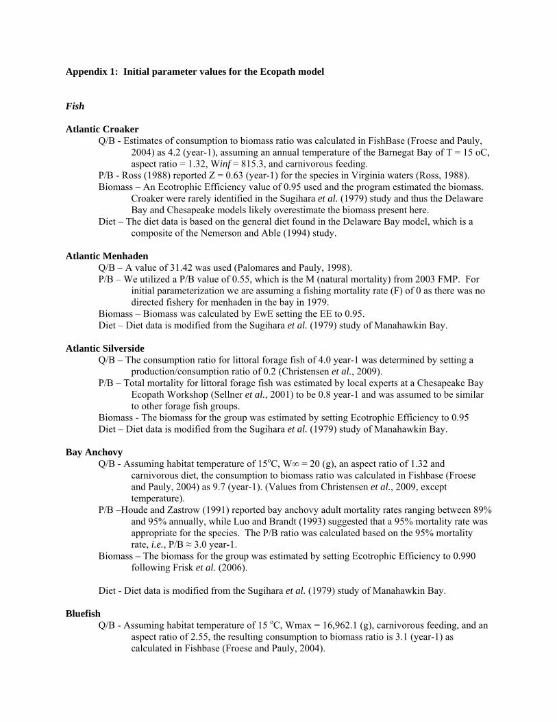
Appendix 1: Initial parameter values for the Ecopath model

Fish Atlantic Croaker

Q/B - Estimates of consumption to biomass ratio was calculated in FishBase (Froese and Pauly, 2004) as 4.2 (year-1), assuming an annual temperature of the Barnegat Bay of T = 15 oC, aspect ratio = 1.32, Winf = 815.3, and carnivorous feeding.

P/B - Ross (1988) reported Z = 0.63 (year-1) for the species in Virginia waters (Ross, 1988). Biomass – An Ecotrophic Efficiency value of 0.95 used and the program estimated the biomass.

Croaker were rarely identified in the Sugihara et al. (1979) study and thus the Delaware Bay and Chesapeake models likely overestimate the biomass present here.

Diet – The diet data is based on the general diet found in the Delaware Bay model, which is a composite of the Nemerson and Able (1994) study.

Atlantic Menhaden Q/B – A value of 31.42 was used (Palomares and Pauly, 1998).

P/B – We utilized a P/B value of 0.55, which is the M (natural mortality) from 2003 FMP. For initial parameterization we are assuming a fishing mortality rate (F) of 0 as there was no directed fishery for menhaden in the bay in 1979.

Biomass – Biomass was calculated by EwE setting the EE to 0.95. Diet – Diet data is modified from the Sugihara et al. (1979) study of Manahawkin Bay.

Atlantic Silverside

Q/B – The consumption ratio for littoral forage fish of 4.0 year-1 was determined by setting a production/consumption ratio of 0.2 (Christensen et al., 2009).

P/B – Total mortality for littoral forage fish was estimated by local experts at a Chesapeake Bay Ecopath Workshop (Sellner et al., 2001) to be 0.8 year-1 and was assumed to be similar to other forage fish groups.

Biomass - The biomass for the group was estimated by setting Ecotrophic Efficiency to 0.95 Diet – Diet data is modified from the Sugihara et al. (1979) study of Manahawkin Bay.

Bay Anchovy Q/B - Assuming habitat temperature of 15oC, W∞ = 20 (g), an aspect ratio of 1.32 and

carnivorous diet, the consumption to biomass ratio was calculated in Fishbase (Froese and Pauly, 2004) as 9.7 (year-1). (Values from Christensen et al., 2009, except temperature).

P/B –Houde and Zastrow (1991) reported bay anchovy adult mortality rates ranging between 89% and 95% annually, while Luo and Brandt (1993) suggested that a 95% mortality rate was appropriate for the species. The P/B ratio was calculated based on the 95% mortality rate, i.e., P/B ≈ 3.0 year-1.

Biomass – The biomass for the group was estimated by setting Ecotrophic Efficiency to 0.990 following Frisk et al. (2006).

Diet - Diet data is modified from the Sugihara et al. (1979) study of Manahawkin Bay.

Bluefish Q/B - Assuming habitat temperature of 15 oC, Wmax = 16,962.1 (g), carnivorous feeding, and an

aspect ratio of 2.55, the resulting consumption to biomass ratio is 3.1 (year-1) as calculated in Fishbase (Froese and Pauly, 2004).

P/B – Production/biomass was determined as 0.434 (year-1) based on an natural mortality rate (M) = 0.25 (year-1) (Christensen et al. 2009) and an estimate of fishing mortality (F) = 0.184 (year-1) from the ASMFC assessment (2003(b)).

Biomass – Biomass was calculated by setting the Ecotrophic Efficiency to 0.95. Diet – Diet data is modified from the Sugihara et al. (1979) study of Manahawkin Bay, averaged

for all size classes. Mummichog

Q/B – A value of 3.65 was taken from Pauly (1989). P/B – A value of 1.2 was used, following the best professional judgement value of Frisk et al.

(2006). Biomass- The biomass for the group was estimated by setting Ecotrophic Efficiency to 0.95 as

taken from Christensen et al. (2009). Diet – Diet data is modified from the Sugihara et al. (1979) study of Manahawkin Bay.

River herring

Q/B – A value of 8.4 was used, which is the average of Pauly (1989; 8.63 at temp = 10oC) and Palomares (1991; 8.23 at temp=200C).

P/B - Total mortality for this group was based on the P/B of 0.75 year-1 for alewife in Randall and Minns (2000).

Biomass – Biomass was estimated by EcoPath assuming that the Ecotrophic Efficiency of these species in the Bay was 0.95, following Christensen et al. (2009).

Diet – Diet data is modified from the Sugihara et al.(1979) study of Manahawkin Bay. Spot

Q/B – The consumption to biomass ratio was estimated as 6.2 (year-1) using the model in Fishbase (Froese and Pauly, 2004) assuming a habitat temperature of 15 0C, W∞ = 190g (Piner and Jones, 2004) and an aspect ratio of 1.39 (Christensen et al., 2009).

P/B - Hoenig’s method estimated an M = 0.9 (year-1) given a maximum age of 5 (Piner and Jones, 2004). This is consistent with the total mortality (Z) used in the Frisk et al.(2006) model.

Biomass – Biomass was estimated by EcoPath assuming that the Ecotrophic Efficiency of these species in the Bay was 0.90, following Christensen et al.(2009).

Diet – Diet data is modified from the Sugihara et al. (1979) study of Manahawkin Bay. Striped bass

Q/B - An estimated consumption to biomass ratio of 2.4 (year-1) was based on the empirical relationship provided by Fishbase (Froese and Pauly, 2004), assuming an aspect ratio of 2.31 (Christensen et al.2009), temperature T = 15 0C, and W∞ = 46.6 (kg).

P/B – We utilized a value of 0.40, taken from Christensen et al. (2009). This value assumes an M=.15 (ASMFC from Smith et al 2000), and an F= 0.25 (best professional judgment) for resident bass (1-7 years old).

Biomass – A biomass value of 2.1 t/km2 was taken from Christensen et al. (2009) for resident striped bass.

Diet – Diet data is modified from the Sugihara et al. (1979) study of Manahawkin Bay averaged across all size classes.

Summer Flounder

Q/B- The consumption to biomass ratio of = 2.6 (year-1) was calculated from Froese and Pauly (2004) assuming an aspect ratio of 1.32, Wmax = 12,000 (g) carnivorous feeding, and habitat temperature of 15 oC.

P/B- Following the Christensen et al. (2009) and Frisk et al. (2006) models, we utilized a P/B=0.52 based on the 2002 NFSC determination of M=0.2 and F ranging between 0.24 and 0.32.

Biomass – Biomass was estimated by EcoPath using an Ecotrophic Efficiency of 0.95, following Christensen et al. (2009).

Diet – Diet data is modified from the Sugihara et al. (1979) study of Manahawkin Bay. Weakfish

Q/B - The Q/B ratio of 3.0 (year-1) was estimated using Fishbase (Froese and Pauly, 2004) assuming average habitat temperature of 15 0C, aspect ratio of 1.32, maximum weight W∞ = 6,190 (g) (Lowerre-Barbieri et al., 1995) and carnivorous feeding habitats.

P/B – Total mortality of Z = 0.26 (year-1) was estimated using Hoenig’s method (1983) assuming a longevity of 17 years (Lowerre-Barbieri et al., 1995), sensu Frisk et al. (2006).

Biomass – Biomass was estimated by EcoPath using an Ecotrophic Efficiency of 0.90. Diet – Diet data is modified from the Sugihara et al. (1979) study of Manahawkin Bay, averaged

across all size classes. Winter Flounder

Q/B - The estimated consumption ratio of 3.4 year-1 was derived using the empirical equation in FishBase (Froese and Pauly, 2004), and was calculated assuming that T = 15 °C, Winf = 3,600 g, an aspect ratio of 1.32, and carnivorous diet.

P/B - The P/B estimate for this group of 0.460 year-1 is based on a value given for flatfish off the Atlantic seaboard in Sissenwine (1987).

Biomass – Biomass was estimated by EcoPath using an Ecotrophic Efficiency of 0.95. Diet – Diet data is modified from the Sugihara et al. (1979) study of Manahawkin Bay.

Avifauna Piscivorous seabirds

Q/B - The consumption ratio estimate of 120 year-1 was from data for the piscivorous seabirds group in Preikshot (2007).

P/B - A total mortality estimate for piscivorous seabirds of 0.163 year-1 was based on survival rate values of 85-90% for cormorants and 80-93% for alcids in the northeast Atlantic (ICES, 2000).

Biomass - The biomass estimate for piscivorous seabirds of 0.250 t/km2 was modified from Christensen et al. (2009), which was based on advice provided in a Chesapeake Ecopath Workshop (Sellner et al., 2001).

Diet compositions - The diet composition for piscivorous seabirds was modified from Christensen et al. (2009), modified to reduce predation on menhaden and increase the percentage of imported diet items.

Non-Piscivorous seabirds

Q/B - The consumption ratio estimate of 120 year-1 was from data for the non-piscivorous seabirds group in Preikshot (2007).

P/B - A total mortality estimate for piscivorous seabirds of 0.51 year-1 was taken from the Chesapeake model and was based on annual mortality rate of 37% for mallard males and 44% females (Anderson, 1975).

Biomass - The biomass estimate for piscivorous seabirds of 0.121 t/km2 was taken from Christensen et al. (2009) and was based on advice provided in a Chesapeake Ecopath Workshop (Sellner et al., 2001).

Diet compositions - The diet composition for non-piscivorous seabirds was taken from Christensen et al. (2009).

INVERTEBRATES Blue crabs Q/B- The consumption ratio of 4.0 was taken from the Chesapeake Bay model.

P/B – We utilized a P/B= 1.21 (year-1) as taken from Frisk et al.(2006). This was based on a stock assessment for Delaware Bay that used a natural morality of M = 0.8 (year-1) assuming a lifespan of 4 years (Kahn, 2003) and fishing mortality on total stock (recruits and post recruits) of F = 0.41 (year-1) (2000-2002).

Biomass – We utilized an estimate of 7.2 t/km2, which was the biomass developed for the Delaware Bay stock assessment (Kahn and Helser, 2005)

Diet – The diet was taken from Frisk et al. (2006), averaged across stanzas.

Hard Clams Q/B - The consumption ratio was estimated to be 5.1 year-1 assuming a P/Q = 0.20 as taken from

Christensen et al. (2009). P/B - A total production/biomass ratio of 1.02 year-1 was estimated from an empirical equation of

Thomas Brey, AWI, included in the Ecopath software (see Christensen et al. (2000)] for a description of the algorithm), assuming an average mass of 20 g, water T = 17 °C, non-motile behavior, and an average water depth of 6.5 m.

Biomass – A biomass of 62.2 t/km2 was calculated for Barnegat Bay based on a average density

of 0.28 clams/ft2 (1986/1987 hard clam survey, B Muffley presentation) and an average mass of 20 g (Christensen et al. (2009) P/B calculation).

Diet – Diet taken from Frisk et al. (2006).

Oyster Q/B - The consumption to biomass ratio of 2.0 was taken from Christensen et al. (2009). P/B – A P/B ration of 0.15 year-1 was used based on Christensen et al. (2009). Biomass – As there has not been a reported natural set of oysters in many years a de minimus

biomass of 0.001 t/km2 was entered. Diet – Diet data taken from Christensen et al. (2009). Sea Nettles

Q/B – Matishov and Denisov (1999) found a diurnal consumption rate of 7% of biomass for Aurelia aurita medusa in the Black Sea. This would equate to an annual consumption per unit biomass of 365 x 0.07 = 25.55 year-1. Assuming sea nettle medusa are present in Barnegat Bay during June through September, Q/B can be derived to ≈ 6.5 year-1.

P/B – A P/B of 5.0 year-1 was used here based on the rational found in Christensen et al. (2009). Biomass – A biomass of 0.583t/km2 was taken from Christensen et al. (2009). This was derived

from an average of the Baird and Ulanowicz (1989) seasonal models multiplied by a conversion factor of carbon to wet weight of 0.3% for jellies (Shushkina et al., 2000).

Diet – The sea nettle diet data was taken from Christensen et al. (2009).

Ctenophores Q/B and P/B – Shushkina et al. (1989) found that ctenophores in their study had growth rates 1.5

to 2 times greater than jellies. Therefore, the P/B and Q/B values for ctenophores were the values for sea nettles multiplied by 1.75; P/B was 8.800 year-1 and Q/B was 11.38 year-1.

Biomass – A biomass of 3.4 t/km2 was used based on an estimate from data obtained from the VIMS ChesMMAP survey (Sellner et al., 2001).

Diet - The ctenophore diet data was taken from Christensen et al. (2009). Benthic infauna/epifauna

Q/B – A consumption ration of 5.0 year -1 was estimated by Ecopath after designating a P/Q ration of 0.2, following Christensen et al.(2009).

P/B – A P/B of 1.0 year-1 was taken from Christensen et al.(2009) based on the value for annelids given in Jorgensen et al. (2000).

Biomass – Biomass was estimated by Ecopath based on a group Ecotrophic Efficiency of 0.90, following Christensen et al. (2009).

Diet – Diet data taken from Chesapeake Bay model. Amphipods

Q/B – The values for this group is currently based on the same information as benthic infauna/epifauna.

P/B – The values for this group is currently based on the same information as benthic infauna/epifauna.

Biomass – The values for this group is currently based on the same information as benthic infauna/epifauna.

Diet – The values for this group is currently based on the same information as benthic infauna/epifauna.

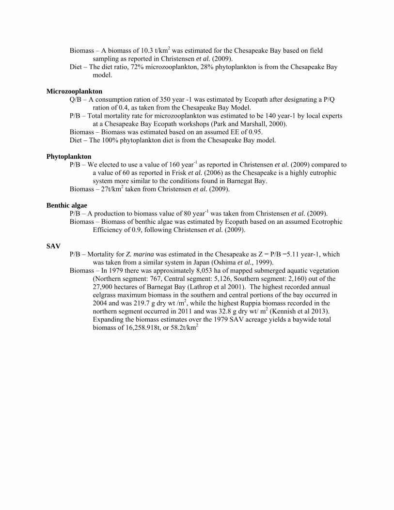
Copepods (Mesozooplankton)

Q/B – A consumption ration of 83.333 year -1 was estimated by Ecopath after designating a P/Q ration of 0.3, following Christensen et al. (2009).

P/B – A mortality rate of 25 year-1 was taken from Christensen et al. (2009), as estimated during the Chesapeake Bay Ecopath Workshop.

Biomass – A biomass of 10.3 t/km2 was estimated for the Chesapeake Bay based on field sampling as reported in Christensen et al. (2009).

Diet – The diet ratio, 72% microzooplankton, 28% phytoplankton is from the Chesapeake Bay model.

Microzooplankton

Q/B – A consumption ration of 350 year -1 was estimated by Ecopath after designating a P/Q ration of 0.4, as taken from the Chesapeake Bay Model.

P/B – Total mortality rate for microzooplankton was estimated to be 140 year-1 by local experts at a Chesapeake Bay Ecopath workshops (Park and Marshall, 2000).

Biomass – Biomass was estimated based on an assumed EE of 0.95. Diet – The 100% phytoplankton diet is from the Chesapeake Bay model.

Phytoplankton

P/B – We elected to use a value of 160 year-1 as reported in Christensen et al. (2009) compared to a value of 60 as reported in Frisk et al. (2006) as the Chesapeake is a highly eutrophic system more similar to the conditions found in Barnegat Bay.

Biomass – 27t/km2 taken from Christensen et al. (2009). Benthic algae

P/B – A production to biomass value of 80 year-1 was taken from Christensen et al. (2009). Biomass – Biomass of benthic algae was estimated by Ecopath based on an assumed Ecotrophic

Efficiency of 0.9, following Christensen et al. (2009). SAV

P/B – Mortality for Z. marina was estimated in the Chesapeake as Z = P/B =5.11 year-1, which was taken from a similar system in Japan (Oshima et al., 1999).

Biomass – In 1979 there was approximately 8,053 ha of mapped submerged aquatic vegetation (Northern segment: 767, Central segment: 5,126, Southern segment: 2,160) out of the 27,900 hectares of Barnegat Bay (Lathrop et al 2001). The highest recorded annual eelgrass maximum biomass in the southern and central portions of the bay occurred in 2004 and was 219.7 g dry wt /m2, while the highest Ruppia biomass recorded in the northern segment occurred in 2011 and was 32.8 g dry wt/ m2 (Kennish et al 2013). Expanding the biomass estimates over the 1979 SAV acreage yields a baywide total biomass of 16,258.918t, or 58.2t/km2

Appendix 2 – Initial Diet Composition Piscivorous

seabirds Non‐piscivorous weakfish

striped bass

summer flounder bluefish

winter flounder

Atlantic silversides

Atlantic croaker spot

Atlantic menhaden

Piscivorous seabirds Non‐piscivorous weakfish 0.0056 0.816 0.013 striped bass 0.0166 summer flounder 0.011 bluefish 0.02 winter flounder 0.0058 0.2 Atlantic silversides 0.017 0.121 0.132 0.087 Atlantic croaker 0.0001 spot 0.016 Atlantic menhaden 0.1 0.255 river herring 0.028 mummichog 0.03 0.36 bay anchovy 0.074 0.86 0.273 0.094 0.018 benthic infauna/epifauna 0.276 0.133 0.06 0.186 0.066 0.742 0.59 0.8 0.509 0.18amphipods 0.004 0.07 0.244 0.25 blue crabs 0.003 0.2 0.103 0.002 hard clams 0.01 0.003 0.157 0.057 oysters copepods 0.154 0.2 0.18 0.338Microzooplankton sea nettles ctenophores benthic algae phytoplankton 0.421SAV 0.128 detritus 0.011 0.009 0.006 0.011 0.012 0.004 0.061import 0.692 0.575

river herring mummichog

bay anchovy

benthic infauna amphipods

blue crabs

hard clams oysters copepods

Micro zoo

sea nettles ctenophores


Non‐piscivorous weakfish striped bass summer flounder bluefish winter flounder Atlantic silversides

Atlantic croaker spot Atlantic menhaden

river herring mummichog 0.564 bay anchovy 0.054benthic infauna/epifauna 0.435 0.256 0.37 0.02 0.02 0.5

amphipods 0.055 0.157 0.044 blue crabs 0.125 hard clams 0.175 oysters copepods 0.5 0.582 0.421 0.666Microzooplankton 0.08 0.08 0.72 0.334sea nettles ctenophores 0.525benthic algae 0.3 0.3 0.05 0.5 phytoplankton 0.005 0.017 0.4 0.4 0.25 0.99 0.28 1 SAV 0.05 detritus 0.005 0.006 0.004 0.2 0.2 0.1 0.25 0.01 import

Date post:	18-May-2018
Category:	Documents
Upload:	vuongkien
View:	217 times
Download:	1 times

Plan 9: Research Barnegat Bay— - The Official Web Site...

Documents