Gerhard Kramm and Nicole Mölders, Planck’s blackbody radiation law 1 Planck’s blackbody radiation law: Presentation in different domains and determination of the related dimensional constants By Gerhard Kramm 1 and Nicole Mölders 1,2 1 University of Alaska Fairbanks, Geophysical Institute, 903 Koyukuk Drive Fairbanks, AK 99775-7320, USA 2 University of Alaska Fairbanks, College of Natural Science and Mathematics, Department of Atmospheric Sciences, 903 Koyukuk Drive Fairbanks, AK 99775-7320, USA Abstract: In this paper the Planck function is derived in the frequency domain using the method of oscillators. It is also presented in the wavelength domain and in the wave number domain. The latter is mainly used in spectroscopy for studying absorption and emission by gases. Also the power law of Stephan and Boltzmann is derived for these various domains. It is shown that this power law is generally independent of the domain in which the Planck function is presented. A formula for the filtered spectrum is also given and expressed in the sense of the power law of Stefan and Boltzmann. Furthermore, based on Wien’s displacement relationship, it is argued that the wavelength at which the maximum of the Planck function presented in the wavelength domain occurs differs from that of the maxima of the other domains by a factor of 76 . 1 . As Planck determined his elementary quantum of action, eventually called the Planck constant, and the Boltzmann constant using Wien’s displacement relationship formulated for the wavelength domain, it is shown that the values of these fundamental constants are not affected by the choice of domain in which the Planck function is presented. Finally, the origin of the Planck constant is discussed. 1. Introduction In 1999 Soffer and Lynch 1 discussed the color sensitivity of the eye in terms of the spectral properties and the photo and chemical stability of available biological materials. Based on Planck’s blackbody radiation law formulated for the wavelength domain and the frequency domain they already illustrated that the peak brightness of the solar spectrum is located in the green range when plotted in wavelength units, but in the near-infrared range when plotted in frequency units. Soffer and Lynch, therefore, stated that the often-quoted notion that evolution led to an optimized eye whose sensitivity peaks where there is most available sunlight is misleading and erroneous. 1 They found that the eye does not appear to be optimized for detection of the available sunlight, including the surprisingly large amount of infrared radiation in the environment. The intensity of blackbody radiation may not only be plotted in wavelength and frequency units, but also in units of wave numbers because the wave number domain is used in the field of spectroscopy for studying the absorption and emission by gases. 2 Students of courses on atmospheric radiation, for instance, often have difficulties to understand why the maximum of Planck’s radiation law presented in the wave number domain differs from that located in the wavelength domain (see Figure 1). In doing so it is important to realize that wave numbers used in spectroscopy differ from those considered in physics by a factor of π 2 .
Transcript
Gerhard Kramm and Nicole Mölders, Planck’s blackbody radiation law 1
Planck’s blackbody radiation law: Presentation in different domains and determination of the related dimensional constants
By Gerhard Kramm1 and Nicole Mölders1,2
1University of Alaska Fairbanks, Geophysical Institute, 903 Koyukuk Drive Fairbanks, AK 99775-7320, USA
2University of Alaska Fairbanks, College of Natural Science and Mathematics,
Department of Atmospheric Sciences, 903 Koyukuk Drive Fairbanks, AK 99775-7320, USA Abstract: In this paper the Planck function is derived in the frequency domain using the method of oscillators. It is also presented in the wavelength domain and in the wave number domain. The latter is mainly used in spectroscopy for studying absorption and emission by gases. Also the power law of Stephan and Boltzmann is derived for these various domains. It is shown that this power law is generally independent of the domain in which the Planck function is presented. A formula for the filtered spectrum is also given and expressed in the sense of the power law of Stefan and Boltzmann. Furthermore, based on Wien’s displacement relationship, it is argued that the wavelength at which the maximum of the Planck function presented in the wavelength domain occurs differs from that of the maxima of the other domains by a factor of 76.1 . As Planck determined his elementary quantum of action, eventually called the Planck constant, and the Boltzmann constant using Wien’s displacement relationship formulated for the wavelength domain, it is shown that the values of these fundamental constants are not affected by the choice of domain in which the Planck function is presented. Finally, the origin of the Planck constant is discussed. 1. Introduction In 1999 Soffer and Lynch1 discussed the color sensitivity of the eye in terms of the spectral properties and the photo and chemical stability of available biological materials. Based on Planck’s blackbody radiation law formulated for the wavelength domain and the frequency domain they already illustrated that the peak brightness of the solar spectrum is located in the green range when plotted in wavelength units, but in the near-infrared range when plotted in frequency units. Soffer and Lynch, therefore, stated that the often-quoted notion that evolution led to an optimized eye whose sensitivity peaks where there is most available sunlight is misleading and erroneous.1 They found that the eye does not appear to be optimized for detection of the available sunlight, including the surprisingly large amount of infrared radiation in the environment.
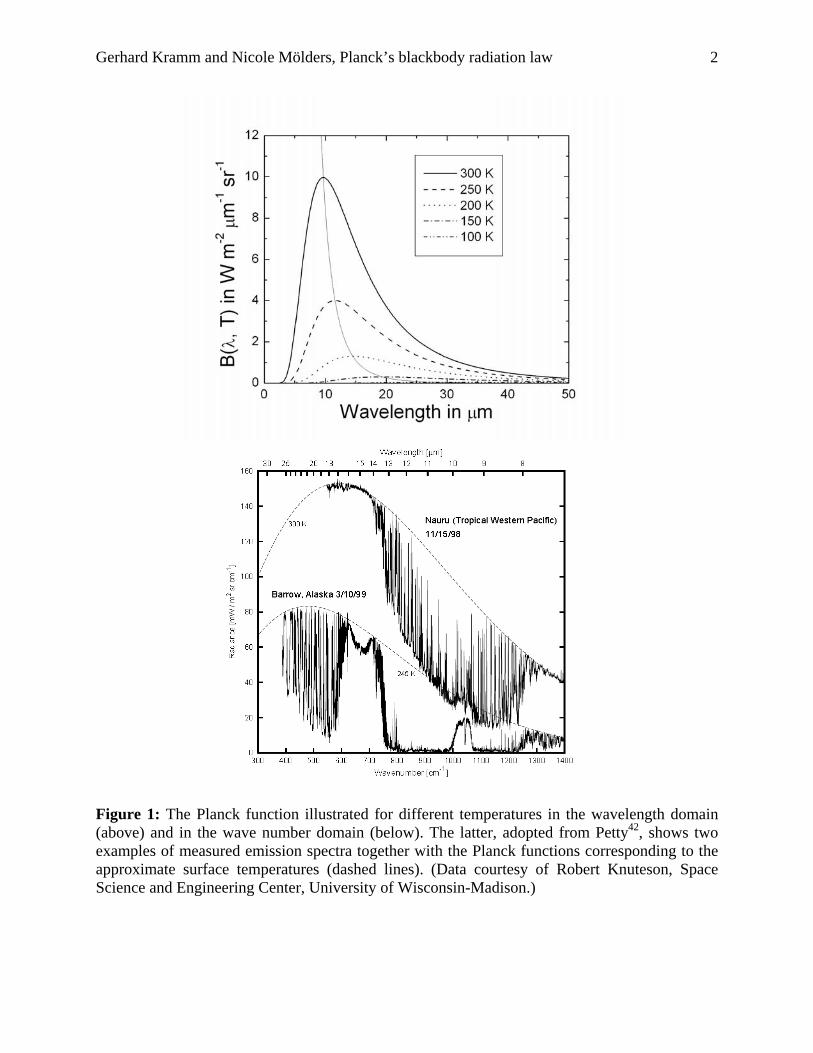
The intensity of blackbody radiation may not only be plotted in wavelength and frequency units, but also in units of wave numbers because the wave number domain is used in the field of spectroscopy for studying the absorption and emission by gases.2 Students of courses on atmospheric radiation, for instance, often have difficulties to understand why the maximum of Planck’s radiation law presented in the wave number domain differs from that located in the wavelength domain (see Figure 1). In doing so it is important to realize that wave numbers used in spectroscopy differ from those considered in physics by a factor of π2 .
Gerhard Kramm and Nicole Mölders, Planck’s blackbody radiation law 2
Figure 1: The Planck function illustrated for different temperatures in the wavelength domain (above) and in the wave number domain (below). The latter, adopted from Petty42, shows two examples of measured emission spectra together with the Planck functions corresponding to the approximate surface temperatures (dashed lines). (Data courtesy of Robert Knuteson, Space Science and Engineering Center, University of Wisconsin-Madison.)
Gerhard Kramm and Nicole Mölders, Planck’s blackbody radiation law 3
Since Planck3 considered – beside the velocity of light in vacuum – Stefan’s constant for estimating the ratio consthk 34 = and Wien’s displacement relationship4 ( ) .constTmax =λ λ , for determining the ratio .constkh = , it is indispensable to show that his way to obtain values for his “Wirkungsquantum”, h , (this means an elementary quantum of action eventually called the Planck constant), and the Boltzmann constant, k , is independent of the domain in which Planck’s radiation law is presented. Here, ( )λλmax is the wavelength at which the maximum of the Planck radiation law occurs in the wavelength domain, and T is the absolute temperature.
Planck introduced an element of energy (see his equation (4)) eventually related to νh (see his §10), where ν is the frequency.3 This means that Planck assumed that energy is quantized, but not light, as often misquoted. A derivation of Planck’s radiation law clearly demonstrates this fact. The quantization of light was introduced by Einstein5 when he related the monochromatic radiation to mutually independent light quanta (or photons) and their magnitude, in principle, to νh that occurs in Planck’s radiation law. Einstein even did not use Planck’s radiation law in its exact manner, but its approximation that fits the exponential law of Wien6 and Paschen7.
Planck’s radiation also plays an important role as the only source function in the radiative transfer equation when a non-scattering medium is in local thermodynamic equilibrium so that a beam of monochromatic intensity passing trough the medium will undergo absorption and emission processes simultaneously, as described by Schwarzschild’s equation.8-11 This is, for instance, the case of the transfer of thermal infrared radiation emitted by the earth and its atmosphere. This kind of radiation plays a prominent role in the physics of climate.8, 12 Therefore, a derivation of this radiation law is very helpful to understand its physical background.
There are various ways to derive Planck’s radiation law. Beside Planck’s original one (that did not fully satisfy him), different derivations were published, for instance, by Einstein13, Bose14, Pauli15, and Kramm and Herbert.16 Einstein’s derivation of Planck’s blackbody radiation law is described, for instance, in the textbooks of Feynman et al.,17 Semat and Albright,18 Rybicki and Lightman,19 and Liou.8 In a very instructive and simplified derivation Einstein introduced the important concept regarding the probability of the emission (including stimulated emission) and/or absorption of radiation. Bose’s derivation is based on a consequent application of the Boltzmann statistics.20 Kramm and Herbert used principles of dimensional analysis in their heuristic derivation of Planck’s law. They showed that a dimensional constant eventually identified as Planck's constant is required to establish a similarity function indispensable to avoid the Rayleigh-Jeans catastrophe in the ultraviolet.21
The following derivation of the Planck function in the frequency domain, presented in Section II, is linked to various sources.3, 15, 19, 23, 24 This derivation is called the method of oscillators15. In Sections III and IV the Planck function is presented in the wavelength domain and in the two wave number domains. The derivation of the power law of Stephan and Boltzmann is presented in Section V. It is shown that this power law is generally independent of the domain in which the Planck function is presented. Also a formula for the filtered spectrum is derived and expressed in the sense of the power law of Stefan and Boltzmann. In Section VI, Wien’s displacement relationship is derived for the various domains. It is shown that ( )λλmax
differs from ( )νλmax of the frequency domain and ( )snmaxλ and ( )pn
maxλ of the two wave number domains used in spectroscopy (superscript sn ) and physics (superscript pn ) by a factor of 76.1 .
Gerhard Kramm and Nicole Mölders, Planck’s blackbody radiation law 4
Fortunately, the values of the fundamental constants, h and k , are not affected by the choice of domain in which the Planck function is presented. The origin of the Planck constant is discussed in Section VII. 2. The Planck function in the frequency domain An example of a perfect blackbody radiation is the “Hohlraumstrahlung” that describes the radiation in a cavity bounded by any emitting and absorbing opaque substances of uniform temperature. According to Kirchhoff’s findings,22 the state of the thermal radiation in such a cavity is entirely independent of the nature and properties of these substances and only depends on the absolute temperature, T , and the frequency, ν (or the radian frequency νπ=ω 2 or the wavelength λ ). The radiation that ranges from ν to ν+ν d contributes to the field of energy within a volume dV , on average, an amount of energy that is proportional to νd and dV expressed by23, 24
( ) ( ) dVdT,UdVdT,UdE ωω=νν= . (1) The quantity ( )T,U ν (or ( )T,U ω ) is called the monochromatic (or spectral) energy density of radiation. According to Planck, in the case of thermal equilibrium, it may be related to the average energy, E , of a harmonic oscillator of the frequency ν located inside the cavity walls by3, 15 ( ) EAT,U =ν , (2)
where A is a constant. The quantities A and E have to be determined.
In the case of the thermal equilibrium, the probability, ( )jEP , to detect a stationary state with an energy jE is given by20
( ) ⎟⎟⎠
⎞⎜⎜⎝
⎛−α=
TkE
expgEP jjj . (3)
Here, α is a constant, jg is the number of stationary states, and 123 KJ103806.1k −−⋅= is the Boltzmann constant. It reflects Boltzmann’s connection between entropy and probability. Analogous to Boltzmann’s formula, we express the probability that a harmonic oscillator occupies the nth level of energy, nE , by
( ) ⎟⎟⎠
⎞⎜⎜⎝
⎛−==
TkE
expCEPP nnn , (4)
where C is another constant. Planck postulated that such an oscillator can only have the amount of energy3
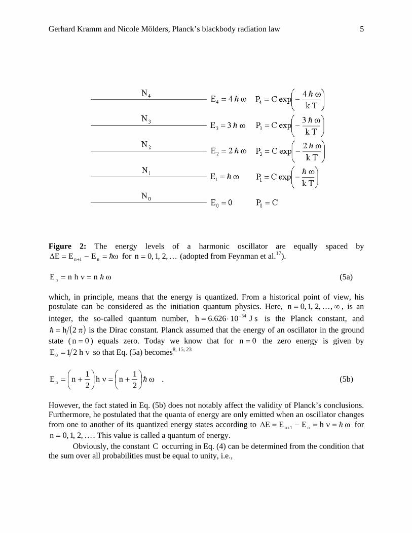
Gerhard Kramm and Nicole Mölders, Planck’s blackbody radiation law 5
Figure 2: The energy levels of a harmonic oscillator are equally spaced by
ω=−=Δ + hn1n EEE for K,2,1,0n = (adopted from Feynman et al.17).
ω=ν= hnhnE n (5a) which, in principle, means that the energy is quantized. From a historical point of view, his postulate can be considered as the initiation quantum physics. Here, ∞= ,,2,1,0n K , is an integer, the so-called quantum number, sJ10626.6h 34−⋅= is the Planck constant, and
( )π= 2hh is the Dirac constant. Planck assumed that the energy of an oscillator in the ground state ( 0n = ) equals zero. Today we know that for 0n = the zero energy is given by
ν= h21E0 so that Eq. (5a) becomes8, 15, 23
ω⎟⎠⎞
⎜⎝⎛ +=ν⎟
⎠⎞
⎜⎝⎛ += h
21nh
21nEn . (5b)
However, the fact stated in Eq. (5b) does not notably affect the validity of Planck’s conclusions. Furthermore, he postulated that the quanta of energy are only emitted when an oscillator changes from one to another of its quantized energy states according to ω=ν=−=Δ + hhEEE n1n for
K,2,1,0n = . This value is called a quantum of energy. Obviously, the constant C occurring in Eq. (4) can be determined from the condition that
the sum over all probabilities must be equal to unity, i.e.,
Gerhard Kramm and Nicole Mölders, Planck’s blackbody radiation law 6
1Tk
EexpC
TkE
expCP0n
n
0n
n
0nn =⎟⎟
⎠
⎞⎜⎜⎝
⎛−=⎟⎟
⎠
⎞⎜⎜⎝
⎛−= ∑∑∑
∞
=
∞
=
∞
=
. (6)
Thus, we have
∑∞
=⎟⎟⎠
⎞⎜⎜⎝
⎛−
=
0n
n
TkEexp
1C . (7)
Now, we consider a lot of oscillators each being a vibrator of frequency ν . Some of these oscillators, namely 0N , will be in the ground state ( 0n = ), 1N will be in the next higher one ( 1n = ), and so forth (see Figure 2). Thus, at the nth energy level we have an energy amount of
nnn NE=ε . The number of harmonic oscillators that occupies a level of energy is related to the corresponding probability by ( )nnn EPNN = so that
∑∞
=⎟⎟⎠
⎞⎜⎜⎝
⎛−
⎟⎟⎠
⎞⎜⎜⎝
⎛−
=⎟⎟⎠
⎞⎜⎜⎝
⎛−==ε
0n
n
nn
nnnnn
TkEexp
TkE
expNE
TkE
expCNENE . (8)
According to
NTk
EexpCNTk
EexpCNNN
))6(.Eqsee(1
0n
n
0n
n
0nn =⎟⎟
⎠
⎞⎜⎜⎝
⎛−=⎟⎟
⎠
⎞⎜⎜⎝
⎛−==
=
∑∑∑∞
=
∞
=
∞
= 44 344 21
, (9)
we may state that N is the total number of harmonic oscillators. The total energy is then given by
∑
∑∑ ∞
=
∞
=∞
=
⎟⎟⎠
⎞⎜⎜⎝
⎛−
⎟⎟⎠
⎞⎜⎜⎝
⎛−
=ε=
0n
n
0n
nn
0nn
TkEexp
TkE
expENE . (10)
From this equation we can infer that the average energy per oscillator in thermal equilibrium as required in Eq. (2) is given by
Gerhard Kramm and Nicole Mölders, Planck’s blackbody radiation law 7
∑
∑∞
=
∞
=
⎟⎟⎠
⎞⎜⎜⎝
⎛−
⎟⎟⎠
⎞⎜⎜⎝
⎛−
==
0n
n
0n
nn
TkEexp
TkE
expE
NEE . (11)
For simplicity we set
∑∞
=⎟⎟⎠
⎞⎜⎜⎝
⎛−=
0n
n
TkEexpZ . (12)
The derivative of Z with respect to T amounts to
∑∑∞
=
∞
=⎟⎟⎠
⎞⎜⎜⎝
⎛−=⎟⎟
⎠
⎞⎜⎜⎝
⎛⎟⎟⎠
⎞⎜⎜⎝
⎛−=
0n
nn2
0n2
nn
TkE
expETk1
TkE
TkE
expdTdZ (13)
or
∑∞
=⎟⎟⎠
⎞⎜⎜⎝
⎛−=
0n
nn
2
TkE
expEdTdZTk . (14)
Combining Eqs. (11) and (14) yields
( )ZlndTdTk
dTdZ
ZTkE 2
2
== . (15)
As nE is quantized (see Eq. (5a)), we obtain
∑∑∞
=
∞
=⎟⎟⎠
⎞⎜⎜⎝
⎛⎟⎟⎠
⎞⎜⎜⎝
⎛ ν−=⎟⎟
⎠
⎞⎜⎜⎝
⎛ ν−=
0n
n
0n Tkhexp
TkhnexpZ . (16)
If we define
⎟⎟⎠
⎞⎜⎜⎝
⎛ ν−=
Tkhexpx , (17)
we will easily recognize that
∑∞
=
=0n
nxZ (18)
Gerhard Kramm and Nicole Mölders, Planck’s blackbody radiation law 8
is a geometric series. As 1x0 <≤ , its sum is given by
⎟⎟⎠
⎞⎜⎜⎝
⎛ ν−−
=−
== ∑∞
=
Tkhexp1
1x1
1xZ0n
n . (19)
Introducing this expression into Eq. (15) yields
( )
⎪⎪⎪⎪
⎭
⎪⎪⎪⎪
⎬
⎫
⎟⎟⎠
⎞⎜⎜⎝
⎛ ν−−
⎟⎟⎠
⎞⎜⎜⎝
⎛ ν−ν
=⎟⎟⎠
⎞⎜⎜⎝
⎛⎟⎟⎠
⎞⎜⎜⎝
⎛ ν⎟⎟⎠
⎞⎜⎜⎝
⎛ ν−−
⎟⎟⎠
⎞⎜⎜⎝
⎛ ν−−
−=
⎪⎭
⎪⎬⎫
⎪⎩
⎪⎨⎧
⎟⎟⎠
⎞⎜⎜⎝
⎛⎟⎟⎠
⎞⎜⎜⎝
⎛ ν−−−==
Tkhexp1
Tkhexph
Tkh
Tkhexp
Tkhexp1
1Tk
Tkhexp1ln
dTdTkZln
dTdTkE
22
22
(20)
or
1Tk
hexp
hE−⎟⎟
⎠
⎞⎜⎜⎝
⎛ νν
= . (21)
Introducing this equation into Eq. (2) provides
( )1
Tkhexp
hAT,U−⎟⎟
⎠
⎞⎜⎜⎝
⎛ νν
=ν . (22)
The expression
1Tk
exp
1
1Tk
hexp
1n−⎟⎟
⎠
⎞⎜⎜⎝
⎛ ω=
−⎟⎟⎠
⎞⎜⎜⎝
⎛ ν=
h (23)
is customarily called the Planck distribution. It may be regarded as a special case of the Bose-Einstein distribution when the chemical potential of a “gas” of photons is given by 0=μ .14, 19, 24,
25 Now, we have to determine the constant A . It can be inferred from the classical
blackbody radiation law,
Gerhard Kramm and Nicole Mölders, Planck’s blackbody radiation law 9
( ) Tkc
8T,U 3
2νπ=ν , (24)
where 18 sm10998.2c −⋅= is the velocity of light in vacuum. This radiation law was first derived by Rayleigh26, 27 using principles of classical statistics, with a correction by Jeans28 today known as Rayleigh-Jeans law. Note that Lorentz29 derived it in a somewhat different way. This classical radiation law fulfills both (a) Kirchhoff’s findings regarding the state of the thermal radiation in a cavity, and (b) the requirements of Wien’s displacement law that reads3, 15, 21 ( ) ( )TfT,U 3 νν∝ν . (25)
For small frequencies at relatively high temperature, this formula works well. It was experimentally proofed by Lummer and Pringsheim30 and Rubens and Kurlbaum.31, 32 Thus, Planck3 already stated that the law of the energy distribution within the normal spectrum derived by Wien6 on the basis of molecular kinetic considerations (experimentally proved by Paschen7) and later deduced by himself on the basis of the theory of the electromagnetic radiation and the 2nd law of thermodynamics33, 34 cannot be generally valid. However, the Rayleigh-Jeans law cannot be correct for high values of ν because for ∞→ν the monochromatic energy density, ( )T,U ν , would tend to infinity.5 Ehrenfest coined this behavior the Rayleigh-Jeans catastrophe
in the ultraviolet.21 In the following we consider Planck’s formula in the red range for which the Rayleigh-Jeans law is valid. This consideration is related to Ehrenfest’s red requirement.21
For 0→ν Eq. (22) provides ( ) 00T,U →ν . Thus, we have to use the de l’Hospital’s rule. For ( ) ν=ν hAf and ( ) ( )( ) 1Tkhexpg −ν=ν we obtain
( )( ) TkA
Tkhexp
Tkh
hAlim'g'flim
00=
⎟⎟⎠
⎞⎜⎜⎝
⎛ ν=
νν
→ν→ν . (26)
Comparing Eqs.(24) and (26) yields
3
2
c8A νπ
= , (27)
as already mentioned by Planck3. Inserting this expression in Eq. (22) leads to3, 15
( )1
Tkhexp
ch8T,U
3
3
−⎟⎟⎠
⎞⎜⎜⎝
⎛ ννπ
=ν . (28)
Consequently, Eq. (1) may be written as
Gerhard Kramm and Nicole Mölders, Planck’s blackbody radiation law 10
dVd1
Tkhexp
ch8dE
3
3 ν−⎟⎟
⎠
⎞⎜⎜⎝
⎛ ννπ
= (29)
or
dVd1
Tkexp
cdE
3
32 ω−⎟⎟
⎠
⎞⎜⎜⎝
⎛ ωω
π=
h
h . (30)
The monochromatic intensity, ( )T,B ν , is generally related to the differential amount of
radiant energy, dE , that crosses an area element dA in directions confined to a differential solid angle Ωd being oriented at an angle θ to the normal of dA ,
( ) dtdddAcosT,BdE νΩθν= , (31) in the time interval between t and dtt + and the frequency interval between ν and ν+ν d . Thus, we obtain
( )
( ) ( )⎪⎪⎪
⎭
⎪⎪⎪
⎬
⎫
ννπ
=νπΩ
θνπ
=
νΩθν=ν−⎟⎟
⎠
⎞⎜⎜⎝
⎛ ννπ
=
=
dVdT,Bc
4ddtc4ddAcosT,B
c4
ddtddAcosT,BdVd1
Tkhexp
ch8dE
dV
3
3
44 344 21
(32)
and, hence,8, 9
( )1
Tkhexp
ch2T,B
3
2
−⎟⎟⎠
⎞⎜⎜⎝
⎛ νν
=ν . (33)
The quantity πΩ
4d in Eq. (32) expresses the probability of radiation propagation in a certain
direction. Using the relationship ( ) ( )( ) νϑν=ϑϑ dT,BdT,B , (34)
where ϑ stands for any variable like radian frequency, ω , wavelength, λ , wave number as defined in spectroscopy, c1ns ν=λ= , or the wave number as defined in physics
Gerhard Kramm and Nicole Mölders, Planck’s blackbody radiation law 11
cc22n p ω=νπ=λπ= , that can be related to the frequency ν via the transformation ( )ϑν , yields then
( ) ( )( )1
Tkexp
c4ddT,BT,B
3
23
−⎟⎟⎠
⎞⎜⎜⎝
⎛ ωω
π=
ων
ων=ωh
h (35)
Equations (33) and (35) are customarily called the Planck functions for these two frequency domains. 3. The Planck function in the wavelength domain The frequency domain is given by ],0[ ∞ . As
( ) ( )( ) ( )( ) 2
cT,BddT,BT,B
λλν−=
λν
λν=λ , (36)
we obtain for the Planck function in the wavelength domain ]0,[∞
( )
⎭⎬⎫
⎩⎨⎧
−⎟⎟⎠
⎞⎜⎜⎝
⎛λ
λ
−=λ
1Tk
chexp
ch2T,B5
2
. (37)
4. The Planck function in the wave number domain Since the wave numbers defined in spectroscopy, c1ns ν=λ= , and in physics,
cc22n p ω=νπ=λπ= , differ from each other by the factor of π2 , we obtain two slightly different results: Spectroscopy:
( ) ( )( )1
Tknchexp
nch2dndT,nBT,nB
s
3s2
sss
−⎟⎟⎠
⎞⎜⎜⎝
⎛=
νν= . (38)
Physics:
( ) ( )( )( )
1Tknc
exp
n2
c2dndT,nBT,nB
p
3p
3
2
ppp
−⎟⎟⎠
⎞⎜⎜⎝
⎛π=
νν=
h
h . (39)
Gerhard Kramm and Nicole Mölders, Planck’s blackbody radiation law 12
Equation (38) is illustrated in the lower part of Figure 1 for two different surface temperatures together with two examples of measured emission spectra. 5. The power law of Stefan and Boltzmann Integrating Eq. (35) over all frequencies yields for the total intensity
( ) ( ) ∫∫∞∞
ν−⎟⎟
⎠
⎞⎜⎜⎝
⎛ νν
=νν=0
3
20
d1
Tkhexp
ch2dT,BTB . (40)
Defining Tk
h ν=Χ leads to
( ) ( ) ( )∫∫∞∞
Χ−Χ
Χ=νν=
0
34
32
4
0
d1exp
Thck2dT,BTB , (41)
where the integral amounts to3, 8, 16
( ) 15d
1exp
4
0
3 π=Χ
−ΧΧ
∫∞
. (42)
Thus, Eqs. (41) and (42) provides for the total intensity ( ) 4TTB β= (43)
with
32
44
hc15k2 π
=β . (44)
Since blackbody radiance may be considered as an example of isotropic radiance, we obtain for the radiative flux density also called the irradiance (see Appendix A) ( ) ( ) 4TTBTF βπ=π= (45)
or ( ) 4TTF σ= , (46)
Gerhard Kramm and Nicole Mölders, Planck’s blackbody radiation law 13
where 4128 KsmJ1067.5 −−−−⋅=βπ=σ is the Stefan constant. According to Stefan’s empirical findings35 and Boltzmann’s thermodynamic derivation,36 Eq. (46) is customarily called the power law of Stefan and Boltzmann.
On the other hand, the integration of Eq (37) over all wavelengths yields8, 9
( ) ( ) ∫∫∫∞
∞∞
λ
⎭⎬⎫
⎩⎨⎧
−⎟⎟⎠
⎞⎜⎜⎝
⎛λ
λ
=λ
⎭⎬⎫
⎩⎨⎧
−⎟⎟⎠
⎞⎜⎜⎝
⎛λ
λ
−=λλ=0 5
20
5
20
d1
Tkchexp
ch2d1
Tkchexp
ch2dT,BTB . (47)
By using the definition Tk
chλ
=Χ the total intensity becomes
( ) ( )44
32
44
))42(.Eqsee(15
0
34
32
4
TThc15k2dx
1expT
hck2TB
4
β=π
=−Χ
Χ=
π=
∞
∫44 344 21
, (48)
i.e., Eq. (43) deduced in the frequency domain and Eq. (48) deduced in the wavelength domain provide identical results, and, and hence, ( ) ( ) .const215hck 5324 =πσ= The same is true for the two wave number domains. If we consider the transformation from the frequency domain to any ϑ domain, where ϑ stands for ω , λ , sn , or pn , we have to consider that ( ) ( ) νν=ϑϑ dT,BdT,B . This relationship was used in Eqs. (35), (36), (38), and (39). On the
other hand, according to the theorem for the substitution of variables in an integral, we have
( ) ( )( ) ( )ϑ
ϑϑν
ϑν=νν ∫∫ϑ
ϑ
ν
ν
dd
dT,BdT,B2
1
2
1
, (49)
where ( )ϑν is the transformation from ν to ϑ , ( )11 ϑν=ν , and ( )22 ϑν=ν . The results of these integrals are identical because any variable substitution does not affect the solution of an integral. Thus, the solution is independent of the domain. Consequently, the ratio 34 hk of the two natural constants can be derived using the Stefan constant and the velocity of light in vacuum. One obtains 43834 KsJ10248.1hk −−⋅= . This value is independent of the choice of the domain. Note that Planck3 found 43834 KsJ10168.1hk −−⋅= , i.e., a value being only 4.6 % smaller than the current one. If one of these two natural constants is known, the other one can be determined, too. In accord with Planck,3 we consider Wien’s displacement relationship to determine these constants.
As recently pointed out by Gerlich and Tscheuschner37, the Stefan constant is not a universal constant of physics. Obviously, this σ depends on the quantity β . If we consider, for instance, Rayleigh’s radiation formula26
Gerhard Kramm and Nicole Mölders, Planck’s blackbody radiation law 14
( ) ⎟⎟⎠
⎞⎜⎜⎝
⎛ ν−
νπ=ν
TkhexpTk
c8T,U 3
2
(50)
which satisfies – like the Planck function – Ehrenfest’s requirements in the red and violet ranges21 (for details, see Kramm and Herbert16), the monochromatic intensity will read
( ) ⎟⎟⎠
⎞⎜⎜⎝
⎛ ν−
ν=ν
TkhexpTk
c2T,B 2
2
. (51)
Thus, the total intensity reads
( ) ( ) ( ) ( ) 4R
432
4
0
2432
4
0
T3Thck2dexpT
hck2dT,BTB β=Γ=ΧΧ−Χ=νν= ∫∫
∞∞
(52)
where Tk
h ν=Χ and 32
4
R hck4
=β . Here, the subscript R characterizes the value deduced from
Rayleigh’s radiation formula. This value differs from that obtained with the Planck function by a factor, expressed by β≅πβ=β 308.030 4
R . Thus, in the case of Rayleigh’s radiation formula the value of the Stefan constant would be given by 4128
R KsmJ1075.1308.0 −−−−⋅=σ=σ . If we consider any finite or filtered spectrum ranging, for instance, from 1ν to 2ν , Eq.
(41) will become
( ) ( )4
F
34
32
4
Td1exp
Thck2TB
2
1
2
1β=Χ
−ΧΧ
= ∫Χ
Χ
Χ
Χ , (53)
where the value of the filtered spectrum, Fβ , is defined by
( )∫Χ
Χ
Χ−Χ
Χ=β
2
1
d1exphc
k2 3
32
4
F . (54)
This quantity reflects the real world situations.37 In such a case the Stefan’s constant would become
( ) ( ) σΧΧ=Χ−Χ
Χπ
σ=σ ∫Χ
Χ21F
3
4F ,ed1exp
15 2
1
, (55)
where the characteristic value of the filtered spectrum, ( )21F ,e ΧΧ , is defined by38
Gerhard Kramm and Nicole Mölders, Planck’s blackbody radiation law 15
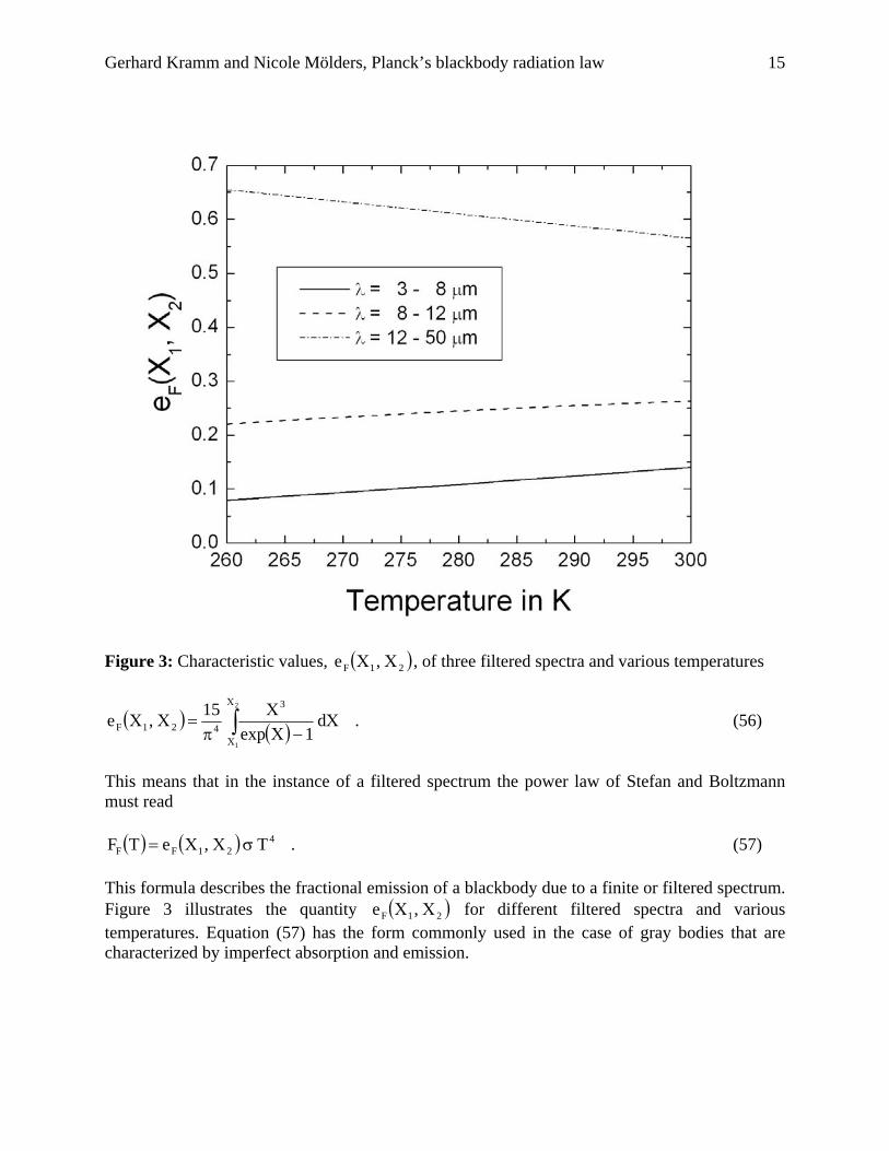
Figure 3: Characteristic values, ( )21F ,e ΧΧ , of three filtered spectra and various temperatures
( ) ( )∫Χ
Χ
Χ−Χ
Χπ
=ΧΧ2
1
d1exp
15,e3
421F . (56)
This means that in the instance of a filtered spectrum the power law of Stefan and Boltzmann must read
( ) ( ) 421FF T,eTF σΧΧ= . (57)
This formula describes the fractional emission of a blackbody due to a finite or filtered spectrum. Figure 3 illustrates the quantity ( )21F ,e ΧΧ for different filtered spectra and various temperatures. Equation (57) has the form commonly used in the case of gray bodies that are characterized by imperfect absorption and emission.
Gerhard Kramm and Nicole Mölders, Planck’s blackbody radiation law 16
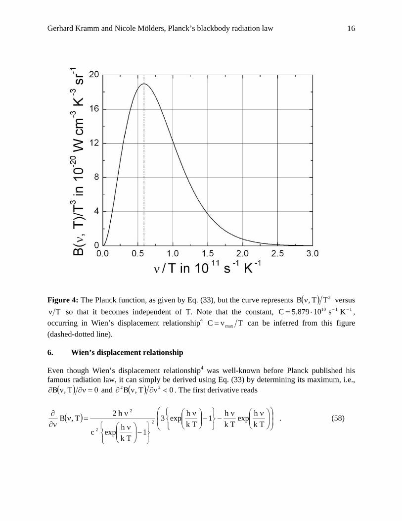
Figure 4: The Planck function, as given by Eq. (33), but the curve represents ( ) 3TT,B ν versus
Tν so that it becomes independent of T. Note that the constant, 1110 Ks10879.5C −−⋅= , occurring in Wien’s displacement relationship4 TC maxν= can be inferred from this figure (dashed-dotted line). 6. Wien’s displacement relationship Even though Wien’s displacement relationship4 was well-known before Planck published his famous radiation law, it can simply be derived using Eq. (33) by determining its maximum, i.e.,
( ) 0T,B =ν∂ν∂ and ( ) 0T,B 22 <ν∂ν∂ . The first derivative reads
( ) ⎟⎟⎠
⎞⎜⎜⎝
⎛⎟⎟⎠
⎞⎜⎜⎝
⎛ νν−
⎭⎬⎫
⎩⎨⎧
−⎟⎟⎠
⎞⎜⎜⎝
⎛ ν
⎭⎬⎫
⎩⎨⎧
−⎟⎟⎠
⎞⎜⎜⎝
⎛ ν
ν=ν
ν∂∂
Tkhexp
Tkh1
Tkhexp3
1Tk
hexpc
h2T,B 2
2
2
. (58)
Gerhard Kramm and Nicole Mölders, Planck’s blackbody radiation law 17
This derivative is only equal to zero when the numerator of the term on the right-hand side of Eq. (58) is equal to zero (the corresponding denominator is larger than zero for ∞<ν<0 ), i.e.,
( ){ } ( )ννν =− xexpx1xexp3 (59) with ( )Tkhx ν=ν . This transcendental function can only be solved numerically. One obtains
8214.2x ≅ν , and in a further step
hkx
Text
ν=ν , (60)
where extν is the frequency at which the extreme (either a minimum or a maximum) of the Planck function in the frequency domain occurs. It can simply be proofed that for this extreme the second derivative fulfills the condition ( ) 0T,B 22 <ν∂ν∂ so that the extreme corresponds to the maximum, maxν . Figure 4 illustrated the value of Tmaxν . If we use that νλ=c we will obtain
( ) Km10098.5kh
xcT 3
max−
ν
ν ⋅≅=λ . (61)
This formula should be called Wien’s displacement relationship, rather than Wien’s displacement law because the latter is customarily used for Eq. (25). For the two different wave number domains, we obtain the same result. Thus, we have
( ) ( ) ( )νλ=λ=λ maxnmax
nmax
sp . (62)
On the other hand, if we consider the Planck function (37) formulated for the wavelength domain, the first derivative will read
( ) ⎟⎟⎠
⎞⎜⎜⎝
⎛⎟⎟⎠
⎞⎜⎜⎝
⎛λλ
−⎭⎬⎫
⎩⎨⎧
−⎟⎟⎠
⎞⎜⎜⎝
⎛λ
⎭⎬⎫
⎩⎨⎧
−⎟⎟⎠
⎞⎜⎜⎝
⎛λ
λ
=λλ∂∂
Tkchexp
Tkch1
Tkchexp5
1Tk
chexp
ch2T,B 2
6
2
. (63)
Again, this derivative is only equal to zero when the numerator of the term on the right-hand side of Eq. (63) equals zero. The corresponding denominator is also larger than zero for ∞<λ<0 . Thus, defining
Tkchx
λ=λ (64)
Gerhard Kramm and Nicole Mölders, Planck’s blackbody radiation law 18
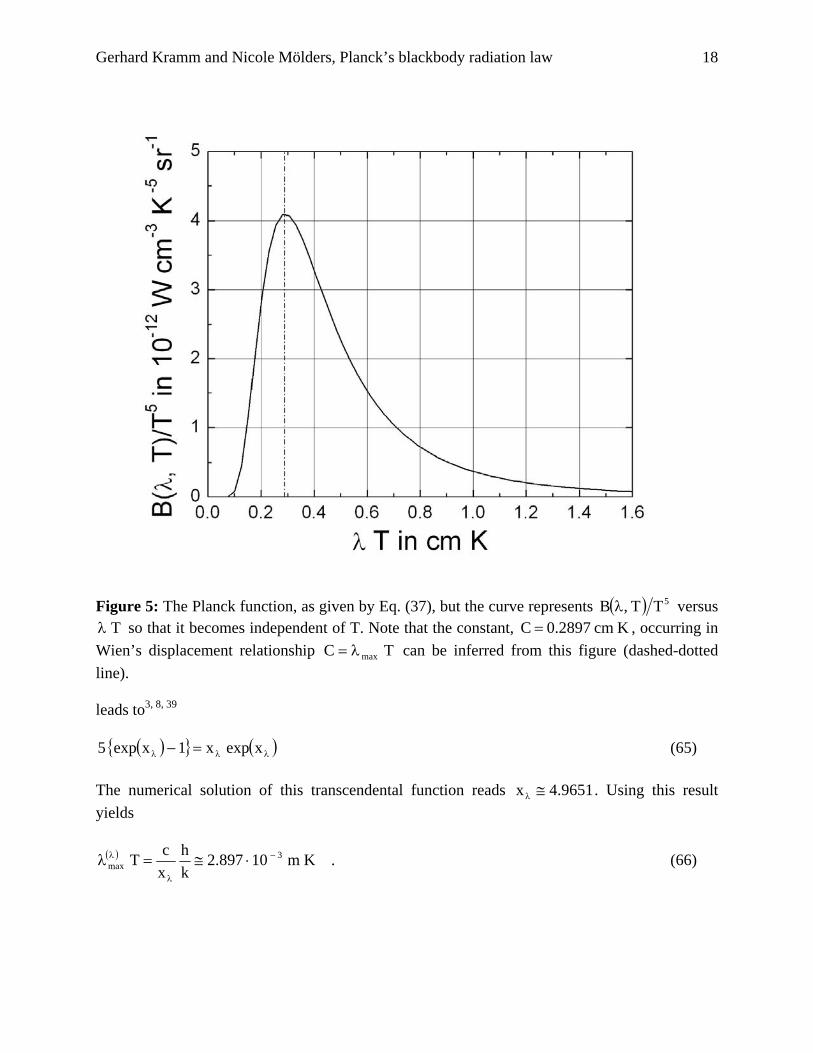
Figure 5: The Planck function, as given by Eq. (37), but the curve represents ( ) 5TT,B λ versus
Tλ so that it becomes independent of T. Note that the constant, Kcm2897.0C = , occurring in Wien’s displacement relationship TC maxλ= can be inferred from this figure (dashed-dotted line). leads to3, 8, 39
( ){ } ( )λλλ =− xexpx1xexp5 (65) The numerical solution of this transcendental function reads 9651.4x ≅λ . Using this result yields
( ) Km10897.2kh
xcT 3
max−
λ
λ ⋅≅=λ . (66)
Gerhard Kramm and Nicole Mölders, Planck’s blackbody radiation law 19
The constant at the right-hand-side of this equation can also be taken from Figure 5. Obviously, we have .constkhc = Note that the requirement ( ) 0T,B 22 <λ∂λ∂ is satisfied for extλ so that this extreme corresponds to a maximum, too.
As expressed by Eqs. (61) and (66), Wien’s displacement relationship, derived for the frequency domain and the wave number domains on the one hand and the wavelength domain on the other hand notably differ from each other being expressed by
( ) ( ) ( )λλ
ν
λν λ≅λ=λ maxmaxmax 76.1xx . (67)
For the blackbody temperature of the sun of K784,5T = Eq. (66) provides ( ) nm500max =λ λ . According to the classification of the visible range by Bruno and Svoronos40, the wavelength of the green region is ranging from nm495 to nm570 . Thus, as stated by Soffer and Lynch,1 the maximum of the solar radiation is located in the green range when considering the wavelength domain. However, according to Kondratyev41 and Petty42 the maximum of solar radiation expressed in wavelength units is located in the light blue range ( nm505485 − ), rather than in the green range ( nm550505 − ). In the case of the other domains the maximum of the solar radiation amounts to a wavelength of ( ) ( ) ( ) nm880max
nmax
nmax
sp =λ=λ=λ ν . Since the near-infrared region is ranging from nm750 to m4 μ ,42 the wavelength of the maximum is located in the near-infrared range, as stated by Soffer and Lynch.1
For an earth’s surface temperature of K300T = the maximum of the terrestrial radiation amounts to ( ) m7.9max μ=λ λ in the wavelength domain (see Figure 1, upper part). Since the atmospheric window is ranging from m3.8 μ to m5.12 μ 2, 8, 42, 43 that corresponds to “spectroscopic” wave numbers ranging from 1cm250,1 − to 1cm800 − , the value of ( )λλmax suggests that the atmospheric window envelops this maximum. However, Eq. (66) provides for the maximum of the terrestrial radiation in the other domains: ( ) ( ) ( ) m0.17max
nmax
nmax
sp μ=λ=λ=λ ν (see Figure 1, lower part). This means that the maximum of the terrestrial radiation at a temperature of K300T = is located beyond the atmospheric window. Note that the spectral region of the atmospheric window ranging from m10 μ to m5.12 μ is the most common band for meteorological satellites because this part is relatively transparent to radiation upwelling from the earth’s surface.2
Nevertheless, either Eq. (61) or (66) can be applied to determine the ratio kh . One obtains sK10808.4kh 11−⋅= . Planck already considered a formula identical with Eq. (66),3 but he used ( ) Km1094.2T 3
max−λ ⋅≅λ , in accord with the empirical findings of Lummer and
Pringsheim30. Thus, he obtained sK10866.4kh 11−⋅= . By taking this value and 43834 KsJ10168.1hk −−⋅= into account, he found: 123 KJ10346.1k −−⋅= and
sJ1055.6h 34−⋅= . Obviously, Planck’s values only slightly differ from the current ones.
Gerhard Kramm and Nicole Mölders, Planck’s blackbody radiation law 20
7. The origin of Planck’s constant In his earlier papers on irreversible radiation processes and the entropy and the temperature of radiative heat, respectively, Planck presented a theoretical derivation of Wien’s radiation law expressed in the wavelength domain [ ]∞,0 by6, 33, 34
( ) ⎟⎟⎠
⎞⎜⎜⎝
⎛λ
−λ
=λTcaexpbc2T,B 5
2
. (68)
He only worked with the constant sK10818.4a 11−⋅= indispensable to make the argument of the in Wien’s exponential law non-dimensional, and sJ10885.6b 34−⋅= . These values hardly differ from those published by him in 1901. Even though Planck did not define it in these two papers33, 34, the constant b is identical with his elementary quantum of action. This means that already in 1896 when Wien published his radiation law a good estimate for the elementary quantum of action could have been obtained.44 Pais, therefore, pointed out that, although Wien did not know this, Wien’s exponential law marked the end of the universal validity of classical physics and the onset of a bizarre turn in science.44
Using the velocity of light in vacuum, 18 sm103c −⋅= , Newton’s gravitational constant, 21311 skgm10685.6 −−−⋅=γ , and his constants a and b Planck introduced natural units of
length, mass, time and temperature by (here expressed in SI units)33
m1013.4cb 35
3−⋅=
γ , (69)
kg1056.5cb 8−⋅=γ
, (70)
s1038.1cb 43
5−⋅=
γ , (71)
and
K1050.3bca 32
5
⋅=γ
. (72)
He concluded that these quantities keep their natural meaning as long as the laws of gravitation, propagation of light in vacuum, and the first and second principles of thermodynamics stay valid, i.e., even measured by different intelligent beings using different methods, these quantities must again result in the same ones. Recently, the number of fundamental constants in physics was debated by Duff, Okun, and Veneziano.45 In contrast to Planck’s four fundamental constants, Okun developed the traditional approach with the first three constants, Veneziano argued in
Gerhard Kramm and Nicole Mölders, Planck’s blackbody radiation law 21
favor of at most two (within superstring theory), while Duff advocated zero. The reader is referred to this detailed discussion.
When he presented his improvement of Wien’s exponential law before the Deutsche Physikalische Gesellschaft (German Physical Society) on October 19, 1900 Planck used the form,24, 44, 46-49
( )1
Taexp
CT,U3
−⎟⎠⎞
⎜⎝⎛ νν
=ν , (73)
where C is another constant. As shown by Kramm and Herbert,16 formula (73) can also be derived by satisfying Ehrenfest’s red requirement21 that leads to the Rayleigh-Jeans law. In contrast this formula, Eq. (28) gives the form of Planck’s radiation law as presented to the German Physical Society on December 14, 1900 and eventually published in 1901.3, 44, 47, 48, 50, 51 This day may be designated the birthday of quantum theory because the elementary quantum of action and the quantum of energy explicitly occurred in Planck’s law.44, 47
Planck’s progress in autumn 1900 may be related to his about-face when he gave up some of his opposition to Boltzmann’s ideas that results in Planck’s use of Boltzmann’s connection between entropy and probability. Klein51 pointed out that Planck had actually begun to consider this connection in his first paper introducing his new distribution46, when he referred to the logarithmic dependence of the entropy on the energy implied by this distribution, saying that such a logarithmic dependence was suggested by the theory of probability. It seems plausible. However, Planck’s formulation of natural units presented before underlines that he had had a view for physical units. Since his constants a and b have the units sK and sJ , respectively, it was surely simple for him to realize that these two constants can be related to each other by another constant having either the units 1JK − or 1KJ − . Like the Boltzmann constant, the latter has the units of the entropy. Planck introduced an additional dimensional constant in his considerations, namely the Boltzmann constant, i.e., kba = (now kha = ). Thus, it is not surprising that the basic relationship Planck referred to was the Boltzmann equation he proceeded to write in the form3
.constWlogkSN += , (74) where the entropy NS of a set of N oscillators of the same frequency whose total energy is NE to the quantity W which is proportional to the probability that the set of oscillators have this value for their total energy.51 We may assume that Planck abandoned his constant a in favor of k , and he determined the latter in his paper of 1901.3 Consequently, replacing the constant a in the exponential function of Eq. (68) by kh results in the non-dimensional argument ( )Tkh ν , i.e., the ratio of two energies. It seems that Planck’s theory presented in his paper of 19013 was formulated in a reverse manner beginning with formula (73).
Planck was not fully satisfied by his derivation. In his Nobel Lecture he stated:52 “However, even if the radiation formula should prove itself to be absolutely accurate, it would still only have, within the significance of a happily chosen interpolation formula, a strictly
Gerhard Kramm and Nicole Mölders, Planck’s blackbody radiation law 22
limited value. For this reason, I busied myself, from then on, that is, from the day of its establishment, with the task of elucidating a true physical character for the formula, and this problem led me automatically to a consideration of the connection between entropy and probability, that is, Boltzmann's trend of ideas; until after some weeks of the most strenuous work of my life, light came into the darkness, and a new undreamed-of perspective opened up before me.” Appendix A The flux density, F , and the intensity, I , are related to each other by
∫Ω
Ωθ= dcosIF , (A1)
where Ω is the entire hemispheric solid angle. As the differential solid angle is given by
φθθ=Ω ddsind , where 20 π≤θ≤ and π≤φ≤ 20 , we have
( ) φθθθφθ= ∫ ∫π π
ddsincos,IF2
0
2
0
(A2)
or
( ) θθθφθφ= ∫ ∫π π
dsincos,IdF2
0
2
0
. (A3)
It is expressed in units of 13 smJ −− or 3mW − . The flux density is also called the irradiance.
In the case of isotropic radiance, i.e., I is independent of θ and φ , we have
θθθφ= ∫ ∫π π
dsincosdIF2
0
2
0
. (A4)
As ( ) θθ=θ cossin2sin21 , Eq. (A4) may also be written as
( )∫ ∫π π
θθφ=2
0
2
0
d2sind2IF . (A5)
Defining θ= 2x yields
( ) ( )[ ] Id2Ixcosd
4Idxxsind
4IF
2
0
2
00
2
0 0
π=φ=−φ=φ= ∫∫∫ ∫ππ
ππ π
. (A6)
Gerhard Kramm and Nicole Mölders, Planck’s blackbody radiation law 23
Note that blackbody radiance is considered as an example of isotropic radiance. Acknowledgements We are grateful to Dr. Glenn E. Shaw, Professor of Physics emeritus at the University of Alaska Fairbanks, Geophysical Institute, for fruitful discussions and helpful suggestions. References 1B.H. Soffer and D.K. Lynch, “Some paradoxes, errors, and resolutions concerning the spectral
optimization of human vision”, Am. J. Phys. 67, 946-953 (1999). 2S.Q. Kidder and T.H. Vonder Haar, “Satellite Meteorology”, (Academic Press, San Diego/New
York/Boston/London/Sydney/Tokyo/Toronto, 1995), 466 pp. 3M. Planck, “Ueber das Gesetz der Energieverteilung im Normalspectrum”, Ann. d. Physik 4,
553-563 (1901, in German). 4W. Wien, “Temperatur und Entropie der Strahlung”, Ann. d. Physik 52, 132-165 (1894, in
German). 5A. Einstein, “Über einen die Erzeugung und Verwandlung des Lichtes betreffenden
heuristischen Gesichtspunkt”, Ann. d. Physik 17, 164-181 (1905, in German). 6W. Wien, “Ueber die Energieverteilung im Emissionsspectrum eines schwarzen Körpers”, Ann.
d. Physik 58, 662-669 (1896, in German). 7F. Paschen, “Ueber die Gesetzmäßigkeiten in den Spectren fester Körper”, Ann. d. Physik 58,
455-492 (1896, in German). 8K.N. Liou, “An Introduction to Atmospheric Radiation”, (Academic Press, Amsterdam/Boston/
London/New York/Oxford/Paris/San Diego/San Francisco/Singapore/Sydney/Tokyo, 2002), 577 pp.
9S. Chandrasekhar, “Radiative Transfer”, (Dover Publications, New York, 1960), 393 pp. 10R.M. Gooody and Y.L. Yung, “Atmospheric Radiation”, (Oxford University Press, New
York/Oxford, 1989), 519 pp. 11J. Lenoble, “Atmospheric Radiative Transfer”, (A. Deepak Publishing, Hampton, VA, 1993),
532 pp. 12J.P. Peixoto and A.H. Oort, “Physics of Climate”, (Springer, New York/Berlin/Heidelberg,
1992), 520 pp. 13A. Einstein, “Zur Quantentheorie der Strahlung”, Physik. Zeitschr. XVIII, 121-128 (1917, in
German). 14S. N. Bose, “Plancks Gesetz und Lichtquantenhypothese”, Z. Phys. 26, 178-181 (1924, in
German). 15W. Pauli, “Statistical Mechanics” (Vol. 4 of Pauli Lectures on Physics), (MIT Press,
Cambridge, MA, 1973), 173 pp. 16G. Kramm and F. Herbert, “Heuristic derivation of blackbody radiation laws using principles of
dimensional analysis”, J. Calcutta Math. Soc. 2 (2), 1-20 (2006). 17R.P. Feynman, R.B. Leighton, and M. Sands, “The Feynman Lectures on Physics- Vol. 1”,
(Addison-Wesley Publishers, Reading, MA/Palo Alto/London, 1963). 18H. Semat and J.R. Albright, “Introduction to Atomic and Nuclear Physics”, (Holt, Rinehart &
Winston, Inc., New York/Chicago/San Francisco/Atlanta/Dallas/Montreal/Toronto/London/ Sydney, 1972), 712 pp.
Gerhard Kramm and Nicole Mölders, Planck’s blackbody radiation law 24
19G.B. Rybicki and A. P. Lightman, “Radiative Processes in Astrophysics”, (Wiley-VCH, Weinheim, Germany, 2004), 400 pp.
20L. Boltzmann, “Über die Beziehung zwischen dem zweiten Hauptsatz der mechanischen Wärmetheorie und der Wahrscheinlichkeitsrechnung respektive den Sätzen über das Wärmegleichgewicht”, Wiener Ber. 76, 373-435 (1877, in German).
21P. Ehrenfest, “Welche Züge der Lichtquantenhypothese spielen in der Theorie der Wärmestrahlung eine wesentliche Rolle”, Ann. d. Physik 36, 91-118 (1911, in German).
22G. Kirchhoff, “Ueber das Verhältniss zwischen dem Emissionsvermögen und dem Absorptionsvermögen für Wärme und Licht”, Ann. d. Physik u. Chemie 109, 275-301 (1860, in German).
23W. Döring, “Atomphysik und Quantenmechanik: I. Grundlagen”, (Walter de Gruyter, Berlin/New York, 1973), 389 pp. (in German).
24L.D. Landau and E.M. Lifshitz, “Course of Theoretical Physics – Vol. 5: Statististical Physics”, (Pergamon Press, Oxford/New York/Toronto/Sydney/Paris/Frankfurt, 1980), 544 pp.
25A. Einstein, “Quantentheorie des einatomigen idealen Gases”, Sitzungsber. Preuß. Akad. Wiss., Berlin, 262-267 (1924); “Zweite Abhandlung”, Sitzungsber. Preuß. Akad. Wiss., Berlin, 3-14 (1925); “Quantentheorie des idealen Gases”, Sitzungsber. Preuß. Akad. Wiss., Berlin, 18-25 (1925, in German; as cited by Rechenberg48).
26Lord Rayleigh (J. W. Strutt), “Remarks upon the law of complete radiation”, Phil. Mag. 49, 539-540 (1900).
27Lord Rayleigh, “The dynamical theory of gases and of radiation”, Nature 72, 54-55 (1905). 28J. H. Jeans, “On the laws of radiation”, Proc. Royal Soc. A 76, 546-567 (1905). 29H. A. Lorentz, “On the emission and absorption by metals of rays of heat of great wave-
length”, Proc. Acad. Amsterdam 5, 666-685 (1903). 30O. Lummer and E. Pringsheim, “Über die Strahlung des schwarzen Körpers für lange Wellen”,
Verh. d. Deutsch. Phys. Ges. 2, 163-180 (1900, in German). 31H. Rubens and R. Kurlbaum, “Über die Emission langwelliger Wärmestrahlen durch den
schwarzen Körper bei verschiedenen Temperaturen”, Sitzungsber. d. K. Akad. d. Wissensch. Berlin vom 25. Oktober 1900, 929-941 (in German).
32H. Rubens and R. Kurlbaum, “Anwendung der Methode der Reststrahlen zur Prüfung des Strahlungsgesetzes”, Ann. d. Physik 4, 649-666 (1901, in German).
33M. Planck, “Über irreversible Strahlungsvorgange”, Ann. d. Physik 1, 69-122 (1900, in German).
34M. Planck, “Entropie und Temperatur strahlender Wärme”, Ann. d. Physik 1, 719-737 (1900, in German).
35J. Stefan, “Über die Beziehung zwischen der Wärmestrahlung und der Temperatur”, Wiener Ber. II, 79, 391-428 (1879, in German).
36L. Boltzmann, “Ableitung des Stefan’schen Gesetzes, betreffend die Abhängigkeit der Wärmestrahlung von der Temperatur aus der electromagnetischen Lichttheorie”, Wiedemann’s Annalen 22, 291-294 (1884, in German).
37G. Gerlich and R.D. Tscheuschner, “Falsification of the atmospheric CO2 greenhouse effects within the frame of physics”, arXiv:0707.1161v3 (2007).
39C.F. Bohren and E.E. Clothiaux, “Fundamentals of Atmospheric Radiation”, (Wiley-VCH, Berlin, Germany, 2006), 472 pp.
Gerhard Kramm and Nicole Mölders, Planck’s blackbody radiation law 25
40T.J. Bruno and P.D.N. Svoronos, “CRC Handbook of Fundamental Spectroscopic Correlation Charts”, (CRC Press, Boca Raton, FL, 2005), 240 pp.
41K.YA. Kondratyev, “Radiation in the Atmosphere”, (Academic Press, New York/London, 1969), 912 pp.
42G.W. Petty, “A First Course in Atmospheric Radiation”, (Sundog Publishing, Madison, WI, 2004), 444 pp.
43F. Möller, “Einführung in die Meteorologie, Bd. 2: Physik der Atmosphäre”, (Bibliographisches Institut, Mannheim/Wien/Zürich, 1973), 223 pp. (in German).
44A. Pais, “Introducing Atoms and their Nuclei”, in: L.M. Brown, A. Pais, and Sir B. Pippard, “Twentieth Century Physics – Vol. I”, (Institute of Physics Publishing, Bristol and Philadelphia, and American Institute of Physics Press, New York, 1995), pp. 43-141.
45M.J. Duff, L.B. Okun, and G. Veneziano, “Trialogue on the number of fundamental constants”, arXiv:physics/0110060v3 (2002).
46M. Planck, “Über eine Verbesserung der Wien’schen Spektralgleichung”, Verh. d. Deutsch. Phys. Ges. 2, 202-204 (1900, in German).
47T.S. Kuhn, “Black-Body Theory and the Quantum Discontinuity 1894-1912”, (Oxford University Press, Oxford/New York, 1978), 356 pp.
48H. Rechenberg, “Quanta and Quantum Mechanics”, in: L.M. Brown, A. Pais, and Sir B. Pippard, “Twentieth Century Physics – Vol. I”, (Institute of Physics Publishing, Bristol and Philadelphia, and American Institute of Physics Press, New York, 1995), pp. 143-248.
49D. Giulini, “Es lebe die Unverfrorenheit! Albert Einstein und die Begrundung der Quantentheorie”, arXiv:physics/0512034 (2005).
50M. Planck, “Zur Theorie des Gesetzes der Energieverteilung im Normalspectrum”, Verh. d. Deutsch. Phys. Ges. 2, 237-245 (1900, in German).
51M.J. Klein, “Paul Ehrenfest – Volume 1: The Making of a Theoretical Physicist”, (North-Holland Publishing Comp., Amsterdam/London, 1970), 330 pp.
52M. Planck, “The genesis and present state of development of the quantum theory”, Nobel Lecture, June 2, 1920 (http://nobelprize.org/nobel_prizes/physics/laureates/1918/planck-lecture.html).