70
Plane Algebraic Curves Andreas Gathmann Class Notes TU Kaiserslautern 2018
Plane Algebraic CurvesAndreas Gathmann
Class Notes TU Kaiserslautern 2018

Contents
0. Introduction . . . . . . . . . . . . . . . . . . . . . . . . . 31. Affine Curves . . . . . . . . . . . . . . . . . . . . . . . . . 62. Intersection Multiplicities . . . . . . . . . . . . . . . . . . . . . 113. Projective Curves . . . . . . . . . . . . . . . . . . . . . . . 204. Bézout’s Theorem . . . . . . . . . . . . . . . . . . . . . . . 285. Applications of Bézout’s Theorem . . . . . . . . . . . . . . . . . . 336. Functions and Divisors . . . . . . . . . . . . . . . . . . . . . . 417. Elliptic Curves . . . . . . . . . . . . . . . . . . . . . . . . 518. The Riemann-Roch Theorem . . . . . . . . . . . . . . . . . . . . 60
References . . . . . . . . . . . . . . . . . . . . . . . . . . . . 67Index . . . . . . . . . . . . . . . . . . . . . . . . . . . . . 68
0. Introduction 3
0. Introduction
These notes are meant as a gentle introduction to algebraic geometry, a combination of linear algebraand algebra:
(a) In linear algebra (as e. g. in the “Foundations of Mathematics” class [G2]), we study systemsof linear equations in several variables over a fixed ground field K.
(b) In algebra (as e. g. in the “Algebraic Structures” or “Introduction to Algebra” classes [G1,G3]), a central topic are polynomials in one variable over K.
Algebraic geometry combines this by studying systems of polynomial equations in several variablesover K. Of course, such polynomials in several variables occur in many places both in pure math-ematics and in applications. Consequently, algebraic geometry has become a very large and activefield of mathematics with deep connections to many other areas, such as commutative algebra, com-puter algebra, number theory, topology, and complex analysis, just to name a few.
On the one hand, all these connections make algebraic geometry into a very interesting field tostudy — but on the other hand they may also make it hard for the beginner to get started. So to keepeverything digestible, we will restrict ourselves here to the first case that is covered by neither (a) nor(b) above: one polynomial equation in two variables. Its set of solutions in K2 can then be thought ofas a curve in the plane, we can draw it (at least in the case K =R), ask geometric questions about it,and try to answer them with algebraic methods. This restriction will significantly reduce the requiredtheoretical background, but still leads to many interesting results that we will discuss in these notes.
To get a feeling for the kind of problems that one may ask about plane curves, we will now mentiona few of them in this introductory chapter. Their flavor differs a bit depending on the chosen groundfield K.
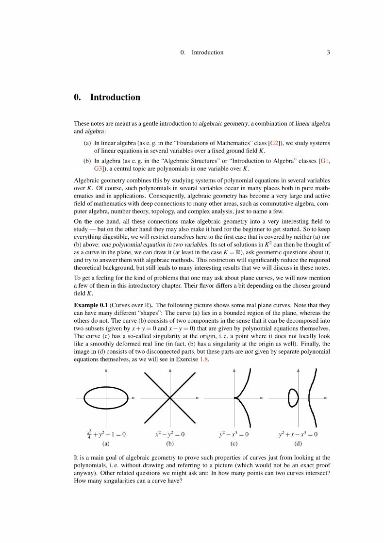
Example 0.1 (Curves over R). The following picture shows some real plane curves. Note that theycan have many different “shapes”: The curve (a) lies in a bounded region of the plane, whereas theothers do not. The curve (b) consists of two components in the sense that it can be decomposed intotwo subsets (given by x+ y = 0 and x− y = 0) that are given by polynomial equations themselves.The curve (c) has a so-called singularity at the origin, i. e. a point where it does not locally looklike a smoothly deformed real line (in fact, (b) has a singularity at the origin as well). Finally, theimage in (d) consists of two disconnected parts, but these parts are not given by separate polynomialequations themselves, as we will see in Exercise 1.8.
x2
4 + y2−1 = 0(a) (b) (c) (d)
y2− x3 = 0x2− y2 = 0 y2 + x− x3 = 0
It is a main goal of algebraic geometry to prove such properties of curves just from looking at thepolynomials, i. e. without drawing and referring to a picture (which would not be an exact proofanyway). Other related questions we might ask are: In how many points can two curves intersect?How many singularities can a curve have?

4 Andreas Gathmann
Example 0.2 (Curves over C). Over the complex numbers, the pictures of curves will look different,since a 1-dimensional complex object is real 2-dimensional, i. e. a surface. Note that we cannot drawsuch a surface as a subset of K2 = C2 = R4 since we would need four dimensions for that. But wecan still get a correct topological picture of the curve itself if we disregard this embedding. Let usshow informally how to do this for the curve with the equation y2 +x−x3 = 0 as in Example 0.1 (d)above; for more details see 5.16.
Note that in this case it is actually possible to write down all the points of the curve explicitly,because the given equation
y2 = x3− x = x(x−1)(x+1)is (almost) solved for y already: We can pick x to be any complex number, and then get two valuesfor y, namely the two square roots of x(x−1)(x+1) — unless x ∈ {−1,0,1}, in which case there isonly one value for y (namely 0).
So one might think that the curve looks like two copies of the complex plane, glued together atthe three points −1,0,1: The complex plane parametrizes the values for x, and the two copies of itcorrespond to the two possible values for y, i. e. to the two roots of the number x(x−1)(x+1).
This is not the correct topological picture however, because a non-zero complex number does nothave a distinguished first and second root that could correspond to the first and second copy of thecomplex plane. Rather, the two roots of a complex number get exchanged if we run around the originonce: If we consider a closed path
z = r eiϕ for 0≤ ϕ ≤ 2π and fixed r > 0
around the complex origin, the square root of this number would have to be defined by√
z =√
r eiϕ2 ,
which gives opposite values at ϕ = 0 and ϕ = 2π . In other words, if x runs around one of the points−1,0,1 (i. e. around a point at which y is the square root of 0), we go from one copy of the plane tothe other. One way to draw this topologically is to cut the two planes along the real intervals (−1,0)and (1,∞), and to glue the two planes along these edges as in the following picture on the left, whereedges with the same letter are meant to be identified. The gluing itself is then visualized best by firstturning one of the planes upside down; this is shown in the picture on the right.
glue
−110
C
C
−110A
B
C
D
A
BC
D
This is now actually a topologically correct picture of the given curve. To make the situation a littlenicer, we can compactify it by adding a point at infinity, which corresponds to identifying the twoplanes at their infinitely far points as well (the precise construction will be described in Chapter 3).This is shown in the picture below, and leads topologically to a torus.

0. Introduction 5
We will show in Proposition 5.16 how such topological pictures can be obtained immediately fromthe given equation of the curve.
Example 0.3 (Curves over Q). The most famous application of algebraic geometry to ground fieldsother than the real or complex numbers is certainly Fermat’s Last Theorem: This is just the statementthat, for n ∈N≥3, the curve given by the equation xn +yn−1 = 0 over the rational numbers has onlythe trivial solutions where x = 0 or y = 0, or equivalently (by setting x = a
c and y = bc for a,b,c ∈ Z
with c 6= 0), that the equation an +bn = cn has no non-trivial solutions over Z. Note that this pictureis very different from the case of the ground fields R or C above. But a large part of the theoryof algebraic curves applies to the rational numbers as well, and in fact the proof of Fermat’s LastTheorem uses concepts of the theory of algebraic curves in many places. So, in some sense, we canview (algebraic) number theory as a part of algebraic geometry.
Example 0.4 (Relations to complex analysis). We have just seen in the examples above that al-gebraic geometry has deep relations to topology and number theory, and it should not come as asurprise that there are many relations to algebraic fields of mathematics such as commutative alge-bra and computer algebra as well. Although it is not within the scope of these notes, let us finish thisintroductory chapter by showing interesting relations to complex analysis as well.
Consider a (sufficiently nice) compactified complex curve, such as a torus as in Example 0.2. Ofcourse, in algebraic geometry one does not only study curves for themselves but also maps betweenthem; and hence we will have to consider “nice” functions on such curves (where “nice” will trans-late into “locally a quotient of polynomials”). What do such functions f look like if they are definedglobally on the whole curve? As the curve is compact, note that the image of f must be a com-pact subset of the complex plane, which means that the absolute value | f | must take a maximumsomewhere. But locally the curve just looks like the complex plane, and by the Maximum ModulusPrinciple [G4, Proposition 6.14] the absolute value of a nice (read: holomorphic) function on thecomplex plane cannot have a local maximum unless it is constant. So we conclude that f must be aconstant function: There are actually no non-trivial nice global functions on a compact curve.
In fact, we will prove this statement in Corollary 6.29 using only algebraic methods, and hence overarbitrary (algebraically closed) ground fields. In a similar way, many interesting results over theground field C can be obtained using both algebraic geometry and complex analysis, with completelydifferent methods, and thus give a close relation between these two branches of mathematics as well.
But let us now start with our study of plane curves. In order to keep these notes as accessibleas possible, we will only assume a basic knowledge of groups, rings, and fields as about to theextent of the “Algebraic Structures” class [G1], but a little more experience in dealing with thesestructures would certainly be advantageous. Very occasionally we will need to assume results fromcommutative algebra that go beyond these prerequisites (marked as “Facts” in the notes), but theywill always be clearly stated and motivated, and provided with a reference. However, in order notto lose this very interesting part of the subject we will nevertheless quite frequently explore therelations of our results to other fields of mathematics in side remarks and excursions (that will thennot be needed afterwards to follow the remaining parts of the notes).

6 Andreas Gathmann
1. Affine Curves
In this first chapter we will introduce plane curves both from an algebraic and a geometric point ofview. As explained in the introduction, they will be given as solutions of polynomial equations. Solet us start by fixing the corresponding notations.
Rings are always assumed to be commutative with a multiplicative neutral element 1. The multi-plicative group of units of a ring R will be denoted by R∗.
Notation 1.1 (Polynomials). Throughout these notes, K will always denote a fixed ground field. ByK[x1, . . . ,xn] we will denote the polynomial ring in n variables x1, . . . ,xn over K, i. e. the ring of finiteformal sums
f = ∑i1,...,in∈N
ai1,...,in xi11 · · · · · x
inn
with all ai1,...,in ∈ K (see e. g. [G1, Chapter 9] how this concept of “formal sums” can be definedin a mathematically rigorous way). Note that we can regard it as an iterated univariate polynomialring since K[x1, . . . ,xn] = K[x1, . . . ,xn−1][xn]. Of course, for a polynomial f as above and a pointP = (c1, . . . ,cn) ∈ Kn, the value of f at P is defined as
f (P) := ∑i1,...,in∈N
ai1,...,in ci11 · · · · · c
inn ∈ K.
Unless stated otherwise, the degree of a term ai1,...,in xi11 · · · · · xin
n as above is meant to be the totaldegree i1 + · · ·+ in in all variables together. The maximum degree occurring in a term with non-zerocoefficient of a polynomial f 6= 0 is called the degree deg f of f . We call F homogeneous if all itsterms have the same degree.
It is easy to see that K[x1, . . . ,xn] is an integral domain, and that deg( f g) = deg f + degg holds forall non-zero polynomials f ,g. The units of K[x1, . . . ,xn] are just the non-zero constant polynomials,which we can identify with K∗ = K\{0}.
Fact 1.2 (Factorial rings). The polynomial ring K[x1, . . . ,xn] is a factorial ring (also called a uniquefactorization domain) [G6, Proposition 8.1 and Remark 8.4]. This means that prime and irreducibleelements agree, and that every non-zero non-unit has a decomposition as a product of irreduciblepolynomials in a unique way (up to permutations, and up to multiplication with units). In the fol-lowing, we will usually use this unique factorization property without mentioning. Note howeverthat, as it is already the case for the integers Z, performing such factorizations in K[x1, . . . ,xn] ex-plicitly or even determining if a given polynomial is irreducible is usually hard.
Definition 1.3 (Affine varieties).(a) For n ∈ N we call An := An
K := Kn the affine n-space over K.
It is customary to use the different notation An for Kn here since Kn is also a K-vector spaceand a ring. We will usually write An
K if we want to ignore these additional structures: Forexample, addition and scalar multiplication are defined on Kn, but not on An
K . The affinespace An
K will be the ambient space for our zero loci of polynomials below.
(b) For a subset S⊂ K[x1, . . . ,xn] of polynomials we call
V (S) := {P ∈ An : f (P) = 0 for all f ∈ S} ⊂ An
the (affine) zero locus of S. Subsets of An of this form are called (affine) varieties. IfS = { f1, . . . , fk} is a finite set, we will write V (S) =V ({ f1, . . . , fk}) also as V ( f1, . . . , fk).
In these notes we will mostly restrict ourselves to zero loci of a single polynomial in twovariables. We will then usually call these variables x and y instead of x1 and x2.

1. Affine Curves 7
Remark 1.4. Obviously, for two polynomials f ,g ∈ K[x,y] we have . . .
(a) V ( f )∪V (g) =V ( f g), as f g(P) = 0 for a point P ∈ A2 if and only if f (P) = 0 or g(P) = 0;
(b) V ( f )∩V (g) =V ( f ,g) by definition.
One would probably expect now that a plane curve is just the zero locus of a polynomial in twovariables. Surprisingly however, it turns out to be convenient to define a (plane) curve as sucha polynomial itself rather than as its zero locus — this will simplify many statements and proofslater on when we want to study curves algebraically, i. e. in terms of their polynomials. Often, wewill denote polynomials by capital instead of small letters if we want to think of them in this way.However, as it is obvious that two polynomials F and G with F = λG for some λ ∈ K∗ have thesame zero locus (and thus determine the same geometric object), we incorporate this already in thedefinition of a curve:
Definition 1.5 (Affine curves).
(a) An (affine plane algebraic) curve is a non-constant polynomial F ∈ K[x,y] modulo units,i. e. modulo the equivalence relation F ∼ G if F = λG for some λ ∈ K∗. We will write itjust as F , not indicating this equivalence class in the notation — this will not lead to anyconfusion.
We call V (F) = {P ∈ A2 : F(P) = 0} the set of points of F .
(b) The degree of a curve is its degree as a polynomial. Curves of degree 1,2,3, . . . are usuallyreferred to as lines, quadrics/conics, cubics, and so on.
(c) A curve F is called irreducible if it is as a polynomial, and reducible otherwise. Similarly,if F = F1
a1 · · · · ·Fakk is the irreducible decomposition of F as a polynomial (see Fact 1.2),
we will also call this the irreducible decomposition of the curve F . The curves F1, . . . ,Fkare then called the (irreducible) components of F and a1, . . . ,ak their multiplicities.
A curve F is called reduced if all its irreducible components have multiplicity 1.
Remark 1.6.
(a) Obviously, the notions of Definition 1.5 are well-defined, i. e. they do not change whenmultiplying a polynomial with a unit in K∗. All our future constructions with curves willalso have this property, and it will be equally obvious in all these cases as well. In thefollowing, we will therefore not mention this fact any more.
(b) In the literature, a curve often refers to the set of points V (F) as in Definition 1.5 (a), i. e. tothe geometric object in A2 rather than to the polynomial F .
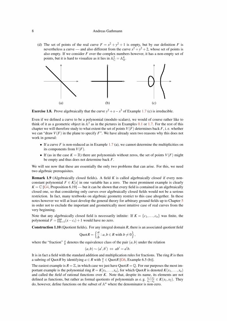
Example 1.7. Especially in the case of the ground field K = R, we will usually visualize a curve Fby drawing its set of points V (F) in the plane — although this does not contain the full informationon the curve, as we will see below.
(a) The curve x+ y is a line, and hence irreducible (as a polynomial of degree 1 cannot be aproduct of two non-constant polynomials). Its square (x+ y)2 has the same set of points asx+ y, but it is a quadric. It is neither irreducible nor reduced.
More generally, it is obvious that curves with the same irreducible components, just withdifferent multiplicities, have the same set of points.
(b) The quadric xy is reducible as well, but it is reduced since it has two irreducible componentsx and y of multiplicity 1.
(c) In contrast to its appearance (see the picture below), the cubic F = y2 +x−x3 is irreducible:If we had F = GH for some non-constant G and H, and thus V (F) = V (G)∪V (H) byRemark 1.4 (a), then one of these factors would have to be a line and the other one a quadric.But F does not contain a line as we can see from the picture.
8 Andreas Gathmann
(d) The set of points of the real curve F = x2 + y2 + 1 is empty, but by our definition F isnevertheless a curve — and also different from the curve x2 + y2 +2, whose set of points isalso empty. If we consider F over the complex numbers however, it has a non-empty set ofpoints, but it is hard to visualize as it lies in A2
C = A4R.
(a) (c)(b)
Exercise 1.8. Prove algebraically that the curve y2 + x− x3 of Example 1.7 (c) is irreducible.
Even if we defined a curve to be a polynomial (modulo scalars), we would of course rather like tothink of it as a geometric object in A2 as in the pictures in Examples 0.1 or 1.7. For the rest of thischapter we will therefore study to what extent the set of points V (F) determines back F , i. e. whetherwe can “draw V (F) in the plane to specify F”. We have already seen two reasons why this does notwork in general:
• If a curve F is non-reduced as in Example 1.7 (a), we cannot determine the multiplicities onits components from V (F).
• If (as in the case K = R) there are polynomials without zeros, the set of points V (F) mightbe empty and thus does not determine back F .
We will see now that these are essentially the only two problems that can arise. For this, we needtwo algebraic prerequisites.
Remark 1.9 (Algebraically closed fields). A field K is called algebraically closed if every non-constant polynomial F ∈ K[x] in one variable has a zero. The most prominent example is clearlyK =C [G4, Proposition 6.19] — but it can be shown that every field is contained in an algebraicallyclosed one, so that considering only curves over algebraically closed fields would not be a seriousrestriction. In fact, many textbooks on algebraic geometry restrict to this case altogether. In thesenotes however we will at least develop the general theory for arbitrary ground fields up to Chapter 5in order not to exclude the important and geometrically most intuitive case of real curves from thevery beginning.
Note that any algebraically closed field is necessarily infinite: If K = {c1, . . . ,cn} was finite, thepolynomial F = ∏
ni=1(x− ci)+1 would have no zero.
Construction 1.10 (Quotient fields). For any integral domain R, there is an associated quotient field
QuotR ={a
b: a,b ∈ R with b 6= 0
},
where the “fraction” ab denotes the equivalence class of the pair (a,b) under the relation
(a,b)∼ (a′,b′) ⇔ ab′ = a′b.
It is in fact a field with the standard addition and multiplication rules for fractions. The ring R is thena subring of QuotR by identifying a ∈ R with a
1 ∈ QuotR [G6, Example 6.5 (b)].
The easiest example is R =Z, in which case we just have QuotR =Q. For our purposes the most im-portant example is the polynomial ring R = K[x1, . . . ,xn], for which QuotR is denoted K(x1, . . . ,xn)and called the field of rational functions over K. Note that, despite its name, its elements are notdefined as functions, but rather as formal quotients of polynomials as e. g. x1+x2
x1−x2∈ K(x1,x2). They
do, however, define functions on the subset of An where the denominator is non-zero.

1. Affine Curves 9
Lemma 1.11. Let F be an affine curve.
(a) If K is algebraically closed then V (F) is infinite.
(b) If K is infinite then A2K\V (F) is infinite.
Proof. As F is not a constant polynomial, it has positive degree in at least one of the variables x andy. By symmetry we may assume that this is x, so that F = anxn + · · ·+a0 for some a0, . . . ,an ∈ K[y]with n > 0 and an 6= 0.
Being non-zero, the polynomial an ∈ K[y] has only finitely many zeros. But K is in any case infiniteby Remark 1.9, hence there are infinitely many y∈K with an(y) 6= 0. For each such y, the polynomialF(x,y) is non-constant in x, so in case (a) there is an x ∈ K with F(x,y) = 0, and in case (b) there isan x ∈ K with F(x,y) 6= 0 (as F( · ,y) has only finitely many zeros). �
01
Proposition 1.12. If two curves F and G have no common component then their intersection V (F,G)is finite.
Proof. By assumption, F and G are coprime in K[x,y]. We claim that they are then also coprimein K(x)[y]. In fact, if they had a common factor in K(x)[y] then after clearing denominators wewould have aF = HF ′ and aG = HG′ for some H,F ′,G′ ∈ K[x,y] of positive y-degree and non-zeroa ∈ K[x]. But then every irreducible factor of a must divide H or both F ′ and G′ in K[x,y], so byreplacing H or both F ′ and G′ by these quotients we arrive at a decomposition F =HF ′ and G=HG′
with H,F ′,G′ ∈ K[x,y] of positive y-degree, in contradiction to F and G being coprime in K[x,y].
Now the ring K(x)[y] as a univariate polynomial ring over a field K(x) is a principal ideal domain[G1, Example 10.22]. So as F,G ∈ K(x)[y] are coprime we can write 1 as a linear combinationof F and G with coefficients in K(x)[y] [G1, Proposition 10.13 (b)], which means after clearingdenominators again that c = DF +EG for some D,E ∈ K[x,y] and non-zero c ∈ K[x].
But if then P ∈V (F,G) we have c(P) = D(P)F(P)+E(P)G(P) = 0. This restricts the x-coordinateof all points P ∈ V (F,G) to the finitely many zeros of c. By symmetry, we then also have onlyfinitely many choices for the y-coordinate, i. e. V (F,G) is finite. �
Corollary 1.13. Let F be a curve over an algebraically closed field. Then for any irreducible curveG we have
G |F ⇔ V (G)⊂V (F).
In particular, the irreducible components of F (but not their multiplicities, see Example 1.7 (a)) canbe recovered from V (F).
Proof.
“⇒” Assume that F = GH for some curve H. If P ∈ V (G), i. e. G(P) = 0, then we also haveF(P) = G(P)H(P) = 0, and hence P ∈V (F).
“⇐” Now assume that V (G) ⊂ V (F). Then V (F,G) = V (G) is infinite by Lemma 1.11 (a). ByProposition 1.12 this means that F and G must have a common component. As G is irre-ducible, this is only possible if G |F . �
Remark 1.14 (Specifying a curve by its set of points). By Corollary1.13, over an algebraically closed field we can specify a curve by givingits set of points together with a multiplicity on each irreducible compo-nent. For example, the picture on the right (where the circle has radius1 and the numbers at the components are their multiplicities) representsthe curve (x2 + y2−1)(x− y)2. (Note however that this is a real picture,but Corollary 1.13 would only hold over C.)
If we do not specify multiplicities in a picture, we usually mean the cor-responding reduced curve, i. e. where all multiplicities are 1.
1
2
10 Andreas Gathmann
Notation 1.15. Due to the above correspondence between a curve F and its set of points V (F), wewill sometimes write:
(a) P ∈ F instead of P ∈V (F), i. e. F(P) = 0 (“P lies on the curve F”);
(b) F ∩G instead of V (F,G) for the points that lie on both F and G;
(c) F ∪G for the curve FG (see Remark 1.4 (a));
(d) G⊂ F instead of G |F .
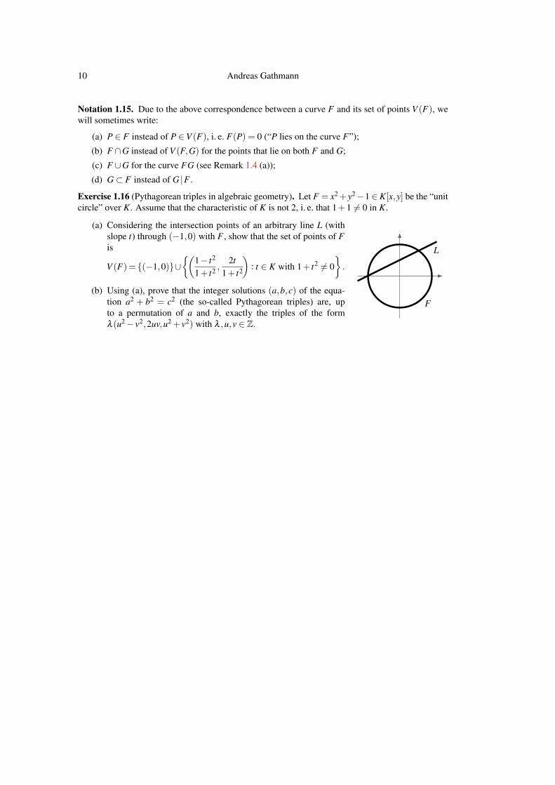
Exercise 1.16 (Pythagorean triples in algebraic geometry). Let F = x2+y2−1∈K[x,y] be the “unitcircle” over K. Assume that the characteristic of K is not 2, i. e. that 1+1 6= 0 in K.
(a) Considering the intersection points of an arbitrary line L (withslope t) through (−1,0) with F , show that the set of points of Fis
V (F)= {(−1,0)}∪{(
1− t2
1+ t2 ,2t
1+ t2
): t ∈ K with 1+ t2 6= 0
}.
(b) Using (a), prove that the integer solutions (a,b,c) of the equa-tion a2 + b2 = c2 (the so-called Pythagorean triples) are, upto a permutation of a and b, exactly the triples of the formλ (u2− v2,2uv,u2 + v2) with λ ,u,v ∈ Z.
F
L

2. Intersection Multiplicities 11
2. Intersection Multiplicities
Let us start our study of curves by introducing the concept of intersection multiplicity, which willbe central throughout these notes. It generalizes the well-known notion of multiplicity of a zeroof a univariate polynomial: If f ∈ K[x] is a polynomial and x0 ∈ K such that f = a(x− x0)
m for apolynomial a ∈ K[x] with a(x0) 6= 0, then f is said to have multiplicity m at x0. As in the followingtwo pictures on the left, a zero of multiplicity 1 means that the graph of f intersects the x-axistransversely, whereas in the case of multiplicity (at least) 2 it is tangent to it. Roughly speaking,higher multiplicities would correspond to graphs for which the x-axis is an even better approximationaround x0.
P
PG
FF
ff
G
x0 x0
multiplicity 1 multiplicity 2multiplicity 1 multiplicity 2f = a(x− x0) f = a(x− x0)
2
In this geometric interpretation, we have already considered how the graph of f intersects the hori-zontal axis locally at the given point, i. e. how the two curves F = y− f and G = y intersect. As inthe picture above on the right, this concept should thus also make sense for arbitrary curves F andG at an intersection point P: If they intersect transversely, i. e. with different tangent directions, wewant to say that they have an intersection multiplicity of 1 at P, whereas equal tangents correspondto higher multiplicities. But of course, the curves F and G might also have “singularities” as e. g.the origin in Example 0.1 (b) and (c), in which case it is not clear a priori how their intersectionmultiplicity can be interpreted or even defined.
So our first task must be to actually construct the intersection multiplicity for arbitrary curves. Forthis we need the following algebraic object that allows us to capture the local geometry of the planearound a point.
Definition 2.1 (Local rings of A2). Let P ∈ A2 be a point.
(a) The local ring of A2 at P is defined as
OP := OA2,P :={
fg
: f ,g ∈ K[x,y] with g(P) 6= 0}⊂ K(x,y).
(b) It admits a well-defined ring homomorphism
OP→ K,fg7→ f (P)
g(P)
which we will call the evaluation map. Its kernel will be denoted by
IP := IA2,P :={
fg
: f ,g ∈ K[x,y] with f (P) = 0 and g(P) 6= 0}⊂OP.
Remark 2.2 (Geometric and algebraic interpretation of local rings). Intuitively, OP describes “nice”(i. e. rational) functions that have a well-defined value at P (determined by the evaluation map), andthus also in a neighborhood of P. Note however that OP does not admit similar evaluation maps

12 Andreas Gathmann
at other points Q 6= P since the denominator of the fractions might vanish there. This explains thename “local ring” from a geometric point of view. The ideal IP in OP describes exactly those localfunctions that have the value 0 at P.
Algebraically, OP is a subring of K(x,y) that contains K[x,y]. As a subring of a field it is an inte-gral domain, and its units are precisely the fractions f
g for which both f and g are non-zero at P.Moreover, just like K[x,y] it is a factorial ring, with the irreducible elements being the irreduciblepolynomials that vanish at P (since the others have become units).
For those who know some commutative algebra we should mention that OP is also a local ring inthe algebraic sense, i. e. that it contains exactly one maximal ideal, namely IP [G6, Definition 6.9]:If I is any ideal in OP that is not a subset of IP then it must contain an element f
g with f (P) 6= 0 andg(P) 6= 0. But this is then a unit since g
f ∈ OP as well, and hence we have I = OP.
In fact, in the algebraic sense OP is just the localization of the polynomial ring K[x,y] at the maximalideal 〈x− x0,y− y0 〉 associated to the point P = (x0,y0) — which also shows that it is a local ring[G6, Corollary 6.10].
Definition 2.3 (Intersection multiplicities). For a point P ∈ A2 and two curves (or polynomials) Fand G we define the intersection multiplicity of F and G at P to be
µP(F,G) := dim OP/〈F,G〉 ∈ N∪{∞},
where dim denotes the dimension as a vector space over K.
As this definition is rather abstract, we should of course figure out how to compute this number, whatits properties are, and why it captures the geometric idea given above. In fact, it is not even obviouswhether µP(F,G) is finite. But let us start with a few simple statements and examples.
Remark 2.4.(a) It is clear from the definitions that an invertible affine coordinate transformation from (x,y)
to
(x′,y′) = (ax+by+ c,dx+ ey+ f ) for a,b,c,d,e, f ∈ K with ae−bd 6= 0
gives us an isomorphism between the local rings OP and OP′ , where P′ is the image point ofP; and between OP/〈F,G〉 and OP′/〈F ′,G′ 〉, where F ′ and G′ are F and G expressed in thenew coordinates x′ and y′. We will often use this invariance to simplify our calculations bypicking suitable coordinates, e. g. such that P = 0 is the origin.
(b) The intersection multiplicity is symmetric: We have µP(F,G) = µP(G,F) for all F and G.
(c) For all F,G,H we have 〈F,G+FH 〉= 〈F,G〉, and thus µP(F,G+FH) = µP(F,G).
In Definition 2.3, we have not required a priori that P actually lies on both curves F and G. However,the intersection multiplicity is at least 1 if and only if it does:
Lemma 2.5. Let P ∈ A2, and let F and G be two curves (or polynomials). We have:
(a) µP(F,G)≥ 1 if and only if P ∈ F ∩G;
(b) µP(F,G) = 1 if and only if 〈F,G〉= IP in OP.
Proof. Assume first that F(P) 6= 0. Then F is a unit in OP, and thus 〈F,G〉=OP, i. e. µP(F,G) = 0.Moreover, we then have P /∈ F and F /∈ IP, proving both (a) and (b) in this case. Of course, the caseG(P) 6= 0 is analogous.
So we may now assume that F(P) = G(P) = 0, i. e. P∈ F∩G. Then the evaluation map at P inducesa well-defined and surjective map OP/〈F,G〉 → K. It follows that µP(F,G)≥ 1, proving (a) in thiscase. Moreover, we have µP(F,G) = 1 if and only if this map is an isomorphism, i. e. if and only if〈F,G〉 is exactly the kernel IP of the evaluation map. �
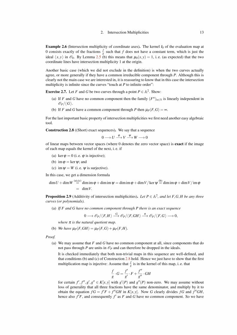
2. Intersection Multiplicities 13
Example 2.6 (Intersection multiplicity of coordinate axes). The kernel I0 of the evaluation map at0 consists exactly of the fractions f
g such that f does not have a constant term, which is just theideal 〈x,y〉 in O0. By Lemma 2.5 (b) this means that µ0(x,y) = 1, i. e. (as expected) that the twocoordinate lines have intersection multiplicity 1 at the origin.
Another basic case (which we did not exclude in the definition) is when the two curves actuallyagree, or more generally if they have a common irreducible component through P. Although this isclearly not the main case we are interested in, it is reassuring to know that in this case the intersectionmultiplicity is infinite since the curves “touch at P to infinite order”:
Exercise 2.7. Let F and G be two curves through a point P ∈ A2. Show:
(a) If F and G have no common component then the family (Fn)n∈N is linearly independent inOP/〈G〉.
(b) If F and G have a common component through P then µP(F,G) = ∞.
For the last important basic property of intersection multiplicities we first need another easy algebraictool.
Construction 2.8 ((Short) exact sequences). We say that a sequence
0−→Uϕ−→V
ψ−→W −→ 0
of linear maps between vector spaces (where 0 denotes the zero vector space) is exact if the imageof each map equals the kernel of the next, i. e. if
(a) kerϕ = 0 (i. e. ϕ is injective);
(b) imϕ = kerψ; and
(c) imψ =W (i. e. ψ is surjective).
In this case, we get a dimension formula
dimU +dimW(a),(c)= dimimϕ +dimimψ = dimimϕ +dimV/kerψ
(b)= dimimϕ +dimV/ imϕ
= dimV.
Proposition 2.9 (Additivity of intersection multiplicities). Let P ∈ A2, and let F,G,H be any threecurves (or polynomials).
(a) If F and G have no common component through P there is an exact sequence
0−→ OP/〈F,H 〉·G−→ OP/〈F,GH 〉 π−→ OP/〈F,G〉 −→ 0,
where π is the natural quotient map.
(b) We have µP(F,GH) = µP(F,G)+µP(F,H).
Proof.
(a) We may assume that F and G have no common component at all, since components that donot pass through P are units in OP and can therefore be dropped in the ideals.
It is checked immediately that both non-trivial maps in this sequence are well-defined, andthat conditions (b) and (c) of Construction 2.8 hold. Hence we just have to show that the firstmultiplication map is injective: Assume that f
g is in the kernel of this map, i. e. that
fg·G =
f ′
g′·F +
f ′′
g′′·GH
for certain f ′, f ′′,g′,g′′ ∈ K[x,y] with g′(P) and g′′(P) non-zero. We may assume withoutloss of generality that all three fractions have the same denominator, and multiply by it toobtain the equation f G = f ′F + f ′′GH in K[x,y]. Now G clearly divides f G and f ′′GH,hence also f ′F , and consequently f ′ as F and G have no common component. So we have
14 Andreas Gathmann
f ′ = aG for some a ∈ K[x,y], and we see that f G = aFG+ f ′′GH. Dividing by G, it followsthat f = aF + f ′′H, so that f and hence also f
g are zero in OP/〈F,H 〉. This shows theinjectivity of the first map.
(b) If F and G have no common component through P the statement follows immediately from(a) by taking dimensions as in Construction 2.8. Otherwise the equation is true as ∞ = ∞ byExercise 2.7 (b). �
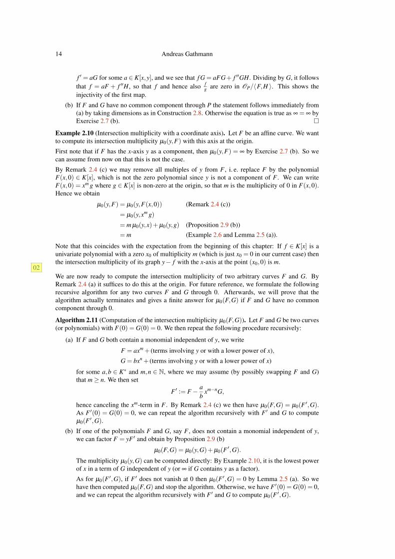
Example 2.10 (Intersection multiplicity with a coordinate axis). Let F be an affine curve. We wantto compute its intersection multiplicity µ0(y,F) with this axis at the origin.
First note that if F has the x-axis y as a component, then µ0(y,F) = ∞ by Exercise 2.7 (b). So wecan assume from now on that this is not the case.
By Remark 2.4 (c) we may remove all multiples of y from F , i. e. replace F by the polynomialF(x,0) ∈ K[x], which is not the zero polynomial since y is not a component of F . We can writeF(x,0) = xm g where g ∈ K[x] is non-zero at the origin, so that m is the multiplicity of 0 in F(x,0).Hence we obtain
µ0(y,F) = µ0(y,F(x,0)) (Remark 2.4 (c))
= µ0(y,xm g)
= m µ0(y,x)+µ0(y,g) (Proposition 2.9 (b))= m (Example 2.6 and Lemma 2.5 (a)).
Note that this coincides with the expectation from the beginning of this chapter: If f ∈ K[x] is aunivariate polynomial with a zero x0 of multiplicity m (which is just x0 = 0 in our current case) thenthe intersection multiplicity of its graph y− f with the x-axis at the point (x0,0) is m.
02We are now ready to compute the intersection multiplicity of two arbitrary curves F and G. ByRemark 2.4 (a) it suffices to do this at the origin. For future reference, we formulate the followingrecursive algorithm for any two curves F and G through 0. Afterwards, we will prove that thealgorithm actually terminates and gives a finite answer for µ0(F,G) if F and G have no commoncomponent through 0.
Algorithm 2.11 (Computation of the intersection multiplicity µ0(F,G)). Let F and G be two curves(or polynomials) with F(0) = G(0) = 0. We then repeat the following procedure recursively:
(a) If F and G both contain a monomial independent of y, we write
F = axm + (terms involving y or with a lower power of x),
G = bxn + (terms involving y or with a lower power of x)
for some a,b ∈ K∗ and m,n ∈ N, where we may assume (by possibly swapping F and G)that m≥ n. We then set
F ′ := F− ab
xm−nG,
hence canceling the xm-term in F . By Remark 2.4 (c) we then have µ0(F,G) = µ0(F ′,G).As F ′(0) = G(0) = 0, we can repeat the algorithm recursively with F ′ and G to computeµ0(F ′,G).
(b) If one of the polynomials F and G, say F , does not contain a monomial independent of y,we can factor F = yF ′ and obtain by Proposition 2.9 (b)
µ0(F,G) = µ0(y,G)+µ0(F ′,G).
The multiplicity µ0(y,G) can be computed directly: By Example 2.10, it is the lowest powerof x in a term of G independent of y (or ∞ if G contains y as a factor).
As for µ0(F ′,G), if F ′ does not vanish at 0 then µ0(F ′,G) = 0 by Lemma 2.5 (a). So wehave then computed µ0(F,G) and stop the algorithm. Otherwise, we have F ′(0) = G(0) = 0,and we can repeat the algorithm recursively with F ′ and G to compute µ0(F ′,G).

2. Intersection Multiplicities 15
Example 2.12. Let us compute the intersection multiplicity µ0(F,G) at the origin of the two curvesF = y2− x3 and G = x2− y3 as in the picture below on the right. We follow Algorithm 2.11 andindicate by (a) and (b) which step we performed each time:
µ0(y2− x3,x2− y3)(a)= µ0(y2− x3 + x(x2− y3),x2− y3)
= µ0(y2− xy3,x2− y3)
(b)= µ0(y,x2− y3)︸ ︷︷ ︸
=2 by 2.10
+µ0(y− xy2,x2− y3)
(b)= 2+µ0(y,x2− y3)︸ ︷︷ ︸
=2 by 2.10
+µ0(1− xy,x2− y3)︸ ︷︷ ︸=0 by 2.5 (a)
= 4.
G
F
Fact 2.13 (Noetherian rings). A ring R is called Noetherian if there is no infinite strictly ascendingchain of ideals I0 ( I1 ( I2 ( · · · in R. It can be shown that the polynomial ring K[x,y] is Noetherian[G6, Proposition 7.13], and that this property is inherited by the local rings OP [G6, Exercise 7.23].
Proposition 2.14 (Finiteness of the intersection multiplicity). Let F and G be two curves (or poly-nomials) that have no common component through the origin. Then Algorithm 2.11 terminates witha finite answer for the intersection multiplicity µ0(F,G).
Proof. First note that the property of not having a common component through 0 is preserved in thealgorithm: In (a) the common components of F ′ and G are the same as those of F and G, and in (b)F ′ and G clearly cannot have a common component through 0 if F = yF ′ and G do not. Hence thecase µ0(y,G) = ∞ in case (b) of the algorithm cannot occur, and thus the algorithm will give a finiteanswer if it terminates.To prove termination, we now consider the ideal 〈F,G〉 in O0 during the algorithm.In case (a) of the algorithm we have 〈F ′,G〉= 〈F,G〉, and the degree of the highest monomial of Findependent of y strictly decreases. Hence, just as in the usual Euclidean algorithm [G1, Proposition10.26], this case (a) can only happen finitely many times in a row before we must be in case (b).In case (b) we then have F = yF ′, and hence 〈F,G〉 ⊂ 〈F ′,G〉. In fact, this inclusion is strict:Otherwise, in the exact sequence
0−→ O0/〈y,G〉·F ′−→ O0/〈F,G〉
π−→ O0/〈F ′,G〉 −→ 0
of Proposition 2.9 (a) the map π would be an isomorphism, and hence the first term O0/〈y,G〉wouldhave to be zero, i. e. µ0(y,G) = 0 — in contradiction to Lemma 2.5 (a).So if the algorithm did not stop, we would get an infinite strictly ascending chain of ideals in O0,which does not exist by Fact 2.13. �
Remark 2.15. If F and G have a common component through 0, Algorithm 2.11 might not termi-nate. For example, for the curves F = x2 and G = xy− x it yields
µ0(x2,xy− x)(a)= µ0(x2 + x(xy− x),xy− x)
= µ0(x2y,xy− x)(b)= µ0(y,xy− x)︸ ︷︷ ︸
=1 by 2.10
+µ0(x2,xy− x),
leading to an infinite loop. However the algorithm is correct in any case, so if it does terminate (witha finite answer), then by Exercise 2.7 (b) we have proven simultaneously with this computation thatF and G have no common component through P.
Exercise 2.16. Draw the real curves F = x2 + y2 + 2y and G = y3x6− y6x2, determine their irre-ducible decompositions, their intersection points, and their intersection multiplicities at these points.

16 Andreas Gathmann
Exercise 2.17.(a) For the curves F = y− x3 and G = y3 − x4, find a polynomial representative of 1
x+1in O0/〈F,G〉, i. e. compute a polynomial f ∈ K[x,y] whose class equals that of 1
x+1 inO0/〈F,G〉.
(b) Prove for arbitrary coprime F and G and any P ∈ A2 that every element of OP/〈F,G〉 has apolynomial representative.Is this statement still true if F and G are not coprime?
Following our algorithm, we can also give an easy and important criterion for when the intersectionmultiplicity is 1.
Notation 2.18 (Homogeneous parts of polynomials). For a polynomial F ∈ K[x,y] of degree d andi = 0, . . . ,d, we define the degree-i part of F to be the sum of all terms of F of degree i. Hence allFi are homogeneous, and we have F = F0 + · · ·+Fd . We call F0 the constant part, F1 the linear part,and Fd the leading part of F .
Proposition 2.19 (Intersection multiplicity 1). Let F and G be two curves (or polynomials) throughthe origin. Then µ0(F,G) = 1 if and only if the linear parts F1 and G1 are linearly independent.
Proof. We prove the statement following Algorithm 2.11, using the notation from there.In case (a), note that F ′1 and G1 are linearly independent if and only if F1 and G1 are, as either F ′1 = F1(if m > n) or F ′1 = F1− a
b G1 (if m = n). Hence we can consider the first time we reach case (b). Asµ0(y,G)> 0 by Lemma 2.5 (a), we have
µ0(F,G) = 1 ⇔ µ0(y,G) = 1 and µ(F ′,G) = 0
⇔ G contains a monomial x1y0 and F ′ contains a constant term(by Example 2.10 and Lemma 2.5 (a))
⇔ G1 = ax+by for some a ∈ K∗,b ∈ K, and F1 = cy for some c ∈ K∗
⇔ F1 and G1 are linearly independent,
where the last implication “⇐” follows since F = yF ′ does not contain a monomial x1y0. �
In fact, Proposition 2.19 has an easy geometric interpretation in thespirit of the beginning of this chapter: F1 and G1 can be thought ofas the linear approximations of F and G around the origin. If these ap-proximations are non-zero, hence lines, they can be thought of as thetangents to the curves as in the picture on the right, and the propositionstates that the intersection multiplicity is 1 if and only if these tangentdirections are not the same.
G
F1G1
F
0
In general, it is the lowest non-zero terms of a curve F that can be considered as the best localapproximation of F around 0. We can use this idea to define tangents to arbitrary curves (i. e. evenif F1 vanishes) as follows.
Definition 2.20 (Tangents and multiplicities of points). Let F be a curve.
(a) The smallest m∈N for which the homogeneous part Fm is non-zero is called the multiplicitym0(F) of F at the origin. Any linear factor of Fm is called a tangent to F at the origin.
(b) For a general point P = (x0,y0) ∈ A2, tangents at P and the multiplicity mP(F) are definedby first shifting coordinates to x′ = x+x0 and y′ = y+y0, and then applying (a) to the origin(x′,y′) = (0,0).
Exercise 2.21. Given a linear coordinate transformation that maps the origin to itself and a curve Fto F ′, show that m0(F) = m0(F ′), and that the transformation maps any tangent of F to a tangent ofF ′.In particular, despite its appearance, Definition 2.20 is independent of the choice of coordinates onA2.

2. Intersection Multiplicities 17
By definition, we clearly have mP(F)> 0 if and only if P∈ F . The most important case of Definition2.20 is when mP(F) = 1, i. e. if there is a non-zero local linear approximation for F around P. Thereis a special terminology for this case.
Definition 2.22 (Smooth and singular points). Let F be a curve.
(a) A point P on F is called smooth or regular if mP(F) = 1. Note that F has then a uniquetangent at P, which we will denote by TPF . For P = 0, it is simply given by the linear partF1 of F .
If P is not a smooth point, i. e. if mP(F)> 1, we say that P is a singular point or a singularityof F . As a special case, a singularity with mP(F) = 2 such that F has two different tangentsthere is called a node.
(b) The curve F is said to be smooth or regular if all its points are smooth. Otherwise, F iscalled singular.
Example 2.23. Let us consider the origin in the real curves in the following picture.
(a) (b) (c) (d)y− x2 y2− x2− x3 y2− x3 x2 + y2
For the case (a), the curve F = y− x2 in (a) has (no constant but) a linear term y. Hence, we havem0(F) = 1, the origin is a smooth point of the curve, and its tangent there is T0F = y.
For the other three curves, the origin is a singular point of multiplicity 2. In (b), this singularity isa node, since the quadratic term is y2− x2 = (y− x)(y+ x), and thus we have the two tangents y− xand y+ x, shown as dashed lines in the picture. The curve in (c) has only one tangent y which is ofmultiplicity 2. Finally, in (d) there is no tangent at all since x2 + y2 does not contain a linear factorover R. Note that, in any case, knowing the tangents of F at the origin (which are easy to compute)tells us to some extent what the curve looks like locally around 0.
With these notations we can now reformulate Proposition 2.19.
Corollary 2.24 (Transverse intersections). Let P be a point in the intersection of two curves F andG. Then µP(F,G) = 1 if and only if P is a smooth point of both F and G, and TPF 6= TPG.
We say in this case that F and G intersect transversely at P.
Remark 2.25 (Additivity of point multiplicities). Note that mP(FG) = mP(F)+mP(G). Hence,any point that lies on at least two (not necessarily distinct) irreducible components has multiplicityat least 2, and is thus a singular point. In particular, all points on a component of multiplicity at least2 (in the sense of Definition 1.5 (c)) are always singular.
To check if a given curve F is smooth, i. e. whether every point P ∈ F is a smooth point of F , thereis a simple criterion that does not require to shift P to the origin first. It uses the (partial) derivatives∂F∂x and ∂F
∂y of F , which can be defined purely formally over an arbitrary ground field and then satisfythe usual rules of differentiation [G1, Exercise 9.10].
Proposition 2.26 (Affine Jacobi Criterion). Let P = (x0,y0) be a point on an affine curve F.
(a) P is a singular point of F if and only if ∂F∂x (P) =
∂F∂y (P) = 0.

18 Andreas Gathmann
(b) If P is a smooth point of F the tangent to F at P is given by
TPF =∂F∂x
(P) · (x− x0)+∂F∂y
(P) · (y− y0).
Proof. Substituting x = x′+ x0 and y = y′+ y0, we can consider F as a polynomial in x′ and y′. Ifwe expand
F = ax′+by′+ (higher order terms in x′ and y′),
then by definition F is singular at (x′,y′) = (0,0), i. e. at P, if and only if a = b = 0. But by the chainrule of differentiation we have
∂F∂x
(P) =∂F∂x′
(0) = a and∂F∂y
(P) =∂F∂y′
(0) = b,
so that (a) follows. Moreover, if F is smooth at P then its tangent is just the term of F linear in x′
and y′, i. e.
ax′+by′ =∂F∂x
(P) · (x− x0)+∂F∂y
(P) · (y− y0),
as claimed in (b). �
Example 2.27. Consider again the real curve F = y2−x2−x3 from Example 2.23 (b). To determineits singular points, we compute the partial derivatives
∂F∂x
=−2x−3x2 and∂F∂y
= 2y.
Its common zeros are (0,0) and (− 23 ,0). But the latter does not lie on the curve, and so we conclude
that the origin is the only singular point of F .03
Smoothness of a curve F at a point P has another important algebraic consequence: It means thatthe containment of ideals containing F in OP can be checked by a simple comparison of intersectionmultiplicities.
Proposition 2.28 (Comparing ideals using intersection multiplicities). Let P be a smooth point ona curve F. Then for any two curves G and H that do not have a common component with F throughP we have
〈F,G〉 ⊂ 〈F,H 〉 in OP ⇔ µP(F,G)≥ µP(F,H).
So in particular, we have 〈F,G〉= 〈F,H 〉 in OP if and only if µP(F,G) = µP(F,H).
Proof.
“⇒”: Clearly, if 〈F,G〉 ⊂ 〈F,H 〉 then µP(F,G) = dimOP/〈F,G〉 ≥ dimOP/〈F,H 〉= µP(F,H).
“⇐”: Let L be a line through P which is not the tangent TPF . Then µP(F,L) = 1 by Corollary 2.24,and hence µP(F,Ln)= n for all n∈N by Proposition 2.9. Let n be the maximum number suchthat 〈F,G〉 ⊂ 〈F,Ln 〉 in OP (this exists since 〈F,G〉 ⊂ OP = 〈F,L0 〉, and 〈F,G〉 ⊂ 〈F,Ln 〉requires n≤ µP(F,G) by the direction “⇒” that we have already shown).
We claim that then 〈F,G〉 = 〈F,Ln 〉 in OP, i. e. that Ln ∈ 〈F,G〉. To see this, note that〈F,G〉 ⊂ 〈F,Ln 〉 implies G = aF + bLn for some a,b ∈ OP. If we had b(P) = 0 it wouldfollow that b ∈ IP = 〈F,L〉 by Lemma 2.5 (b), i. e. b = cF + dL for some c,d ∈ OP, whichmeans that G = aF +(cF + dL)Ln ∈ 〈F,Ln+1 〉 and thus contradicts the maximality of n.Hence b(P) 6= 0, i. e. b is a unit in OP, and we obtain Ln = 1
b (G−aF) ∈ 〈F,G〉 as desired.
Of course, now 〈F,G〉 = 〈F,Ln 〉 implies that µP(F,G) = µP(F,Ln) = n, so that we ob-tain 〈F,G〉 = 〈F,LµP(F,G) 〉. But the same holds for H instead of G, and so the inequalityµP(F,G)≥ µP(F,H) yields
〈F,G〉= 〈F,LµP(F,G) 〉 ⊂ 〈F,LµP(F,H) 〉= 〈F,H 〉. �

2. Intersection Multiplicities 19
Example 2.29. Proposition 2.28 is false without the smoothness assumption on F : For the real curveF = x2−y2 = (x−y)(x+y) (i. e. the union of the two diagonals in A2, with singular point 0), G = x,and H = y, we have 〈F,G〉 = 〈x,y2 〉 and 〈F,H 〉 = 〈y,x2 〉. Hence µ0(F,G) = µ0(F,H) = 2, but〈F,G〉 6= 〈F,H 〉 (since y /∈ 〈x,y2 〉, as otherwise we would have 〈x,y2 〉= 〈x,y〉, in contradiction toµ0(x,y2) = 2 6= 1 = µ0(x,y)).
Remark 2.30 (Smooth curves over R). For the ground field K = R, our results on smooth curveshave an intuitive interpretation:
(a) The Jacobi Criterion of Proposition 2.26 (a) states that P is a smooth point of the curveF if and only if the Implicit Function Theorem [G2, Proposition 27.9] can be applied tothe equation F = 0 around P, so that V (F) is a 1-dimensional submanifold of R2 [G2,Definition 27.17]. Hence, in this case V (F) is locally the graph of a differentiable function(expressing y as a function of x or vice versa), and thus we arrive at the intuitive interpretationof smoothness as “having no sharp corners”.
(b) To interpret Proposition 2.28, let us continue the picture of (a) and consider a local (analytic)coordinate z around P on the 1-dimensional manifold V (F). In accordance with the idea ofintersection multiplicity at the beginning of this chapter, a curve G should have intersectionmultiplicity n with F at P if on F it is locally a function of the form azn in this coordinate,with a non-zero at P (corresponding to a unit in OP). Now if n = µP(F,G)≥ µP(F,H) = mthen in the same way H is of the form bzm, so that bzm = H divides azn = G. This meansthat 〈G〉 ⊂ 〈H 〉 in OP/〈F 〉 (i. e. as functions on F , a point of view that we will discuss indetail starting in Chapter 6) and thus that 〈F,G〉 ⊂ 〈F,H 〉 in OP.
Exercise 2.31 (Cusps). Let P be a point on an affine curve F . We say that P is a cusp if mP(F) = 2,there is exactly one tangent L to F at P, and µP(F,L) = 3.
(a) Give an example of a real curve with a cusp, and draw a picture of it.
(b) If F has a cusp at P, prove that F has only one irreducible component passing through P.
(c) If F and G have a cusp at P, what is the minimum possible value for the intersection multi-plicity µP(F,G)?
Exercise 2.32.(a) Find all singular points of the curve F = (x2+y2−1)3+10x2y2 ∈R[x,y], and determine the
multiplicities and tangents to F at these points.
(b) Show that an irreducible curve F over a field of characteristic 0 has only finitely manysingular points.
Can you find weaker assumptions on F that also imply that F has only finitely many singularpoints?
(c) Show that an irreducible cubic can have at most one singular point, and that over an alge-braically closed field this singularity must be a node or a cusp as in Exercise 2.31.

20 Andreas Gathmann
3. Projective Curves
In the last chapter we have studied the local intersection behavior of curves. Our next major goalwill be to consider the global situation and ask how many intersection points two curves can have intotal, i. e. how many common zeros we find for two polynomials F,G ∈ K[x,y] (where we will counteach such zero with its intersection multiplicity).
For polynomials in one variable, the corresponding question would simply be how many zeros asingle polynomial f ∈ K[x] has. At least if K is algebraically closed, so that f is a product of linearfactors, the answer is then of course that we always get deg f zeros (counted with multiplicities).Hence, in our current case of two polynomials F,G ∈ K[x,y] we would also hope for a result thatdepends only on degF and degG, and not on the chosen polynomials.
However, even in the simplest case when F and G are two distinct lines this will not work, since Fand G might intersect in one point or be parallel (and hence have no intersection point). To fix thissituation, the geometric idea is to add points at infinity to the affine plane A2, so that two lines thatare parallel in A2 will meet there. On the other hand, two non-parallel lines (that intersect already inA2) should not meet at infinity any more as this would then lead to two intersection points. Hence,we have to add one point at infinity for each direction in the affine plane, so that parallel lines withthe same direction meet there, whereas others do not.
This new space with the added points at infinity will be called the projective plane. In the case K =Rwe can also think of it as a compactification of the affine plane A2. It is the goal of this chapter tostudy this process in detail, leading to plane curves that are “compactified” by points at infinity. Fortwo such compactified curves we will then compute the number of intersection points in the nextchapter, and the answer will then indeed depend only on the degrees of the curves.
Remark 3.1 (Geometric idea of projective spaces). Algebraically, the idea for adding points atinfinity is to embed the affine space An in the vector space Kn+1 by prepending a new coordinate(typically called x0) equal to 1, i. e. by the map
An→ Kn+1, (x1, . . . ,xn) 7→ (1,x1, . . . ,xn),
and considering the 1-dimensional linear subspace in Kn+1 spanned by this vector. For example, inthis way a point (c1,c2) ∈A2 corresponds to the line through the origin and (1,c1,c2) ∈ K3, denotedby P in the picture below on the left.
1
x0
1
x2
x0
x1x1
A2 A2(c1,c2)
P
We will define the projective plane as the set of all such 1-dimensional linear subspaces of K3. Itthen consists of all lines through the origin coming from points of A2 as above — together with linescontained in the plane where x0 = 0 that do not arise in this way, such as Q in the picture above.As shown on the right, these lines can be thought of as limits of lines coming from an unboundedsequence of points in A2. They can therefore be interpreted as the “points at infinity” that we werelooking for.
Let us now turn this idea into a precise definition.
3. Projective Curves 21
Definition 3.2 (Projective spaces). For n ∈ N, we define the projective n-space over K as the set ofall 1-dimensional linear subspaces of Kn+1. It is denoted by Pn
K or simply Pn.
Notation 3.3 (Homogeneous coordinates). Obviously, a 1-dimensional linear subspace of Kn+1 isuniquely determined by a spanning non-zero vector in V , with two such vectors giving the samelinear subspace if and only if they are scalar multiples of each other. In other words, we have
Pn = (Kn+1\{0})/∼
with the equivalence relation
(x0, . . . ,xn)∼ (y0, . . . ,yn) :⇔ xi = λyi for some λ ∈ K∗ and all i.
The equivalence class of (x0, . . . ,xn) is usually denoted by (x0 : · · · :xn) ∈ Pn. We call x0, . . . ,xn thehomogeneous or projective coordinates of the point (x0 : · · · :xn). Hence, in this notation for apoint in Pn the numbers x0, . . . ,xn are not all zero, and they are defined only up to a common scalarmultiple.
Remark 3.4 (Geometric interpretation of Pn). There are two ways to interpret the projective spacePn geometrically:
(a) As in Remark 3.1, we can embed the affine space An in Pn by the map
An→ Pn, (x1, . . . ,xn) 7→ (1:x1 : · · · :xn)
whose image is the subset U0 := {(x0 : · · · :xn) : x0 6= 0} of Pn. We will often consider An asa subset of Pn in this way, i. e. by setting x0 = 1. The other coordinates x1, . . . ,xn are thencalled the inhomogeneous or affine coordinates on U0.
The remaining points of Pn are of the form (0:x1 : · · · :xn). By forgetting their coordinate x0(which is zero anyway) they form a set that is naturally bijective to Pn−1, corresponding tothe 1-dimensional linear subspaces of Kn. As in Remark 3.1 we can regard them as pointsat infinity; there is hence one such point for each direction in Kn. In short-hand notation,one often writes this decomposition as Pn = An∪Pn−1 and calls An and Pn−1 the affine andinfinite part of Pn, respectively.
(b) By the symmetry of the homogeneous coordinates, the subsets Ui := {(x0 : · · · :xn) : xi 6= 0}of Pn are naturally bijective to An for all i = 0, . . . ,n, in the same way as for i = 0 in (a). Asevery point of Pn has at least one non-zero coordinate, it lies in one of the Ui, and hence ina subset of Pn that just looks like the ordinary affine space An. In this sense we can say thatprojective space “looks everywhere the same”; the fact that we interpreted the points withx0 = 0 as points as infinity above was just due to our special choice of i = 0 in (a).
Example 3.5. By Remark 3.4 (a), we have P1 = A1 ∪P0. The affine part consists of the points(1:x1) for x1 ∈K, and the infinite part contains the single point (0:1). Denoting this point at infinityby ∞, we can therefore write P1 = A1∪{∞}.
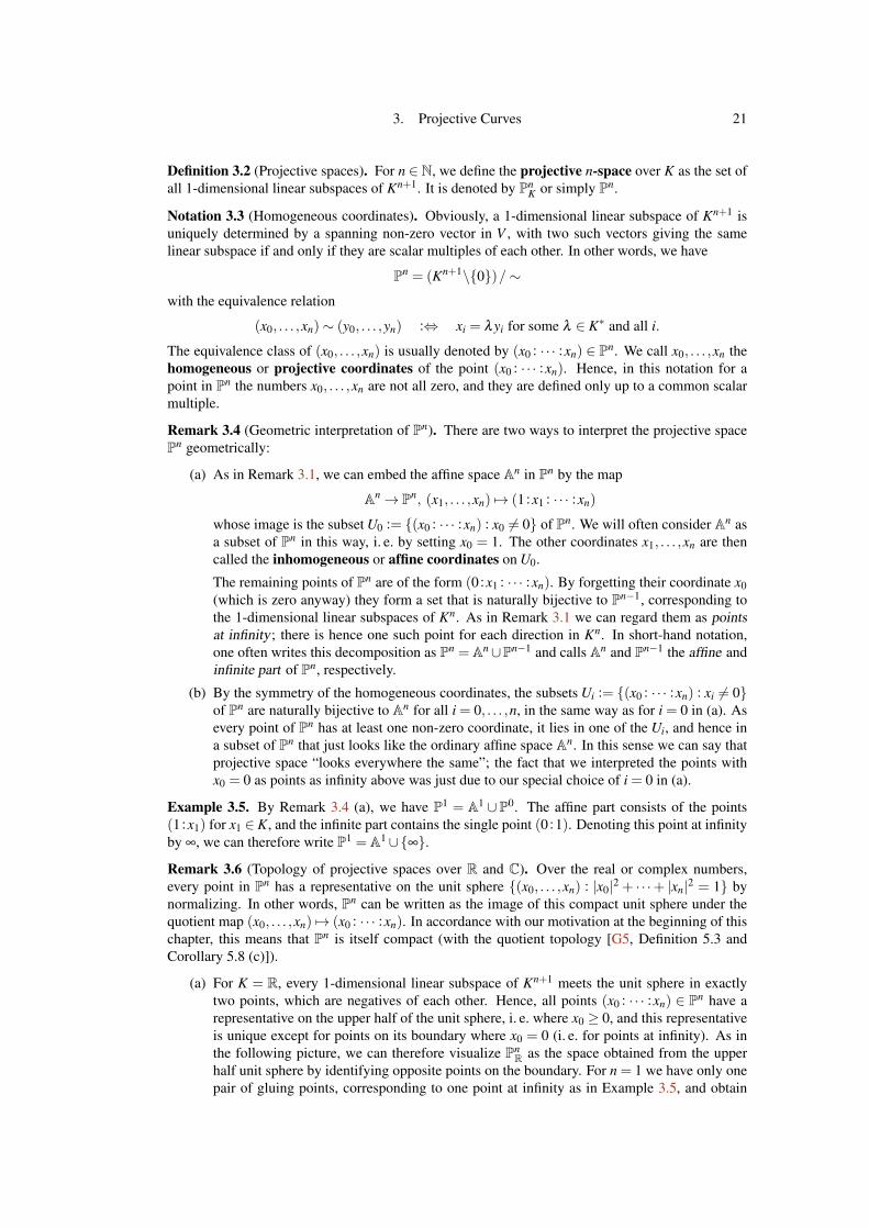
Remark 3.6 (Topology of projective spaces over R and C). Over the real or complex numbers,every point in Pn has a representative on the unit sphere {(x0, . . . ,xn) : |x0|2 + · · ·+ |xn|2 = 1} bynormalizing. In other words, Pn can be written as the image of this compact unit sphere under thequotient map (x0, . . . ,xn) 7→ (x0 : · · · :xn). In accordance with our motivation at the beginning of thischapter, this means that Pn is itself compact (with the quotient topology [G5, Definition 5.3 andCorollary 5.8 (c)]).
(a) For K = R, every 1-dimensional linear subspace of Kn+1 meets the unit sphere in exactlytwo points, which are negatives of each other. Hence, all points (x0 : · · · :xn) ∈ Pn have arepresentative on the upper half of the unit sphere, i. e. where x0 ≥ 0, and this representativeis unique except for points on its boundary where x0 = 0 (i. e. for points at infinity). As inthe following picture, we can therefore visualize Pn
R as the space obtained from the upperhalf unit sphere by identifying opposite points on the boundary. For n = 1 we have only onepair of gluing points, corresponding to one point at infinity as in Example 3.5, and obtain
22 Andreas Gathmann
topologically a circle. For n = 2, each point on the boundary of the upper half unit spherehas to be identified with its negative, which leads to a space that cannot be embedded in R3.
1 x0
x1
glue ∞
x0
x1
x2
glue
P1R P2
R
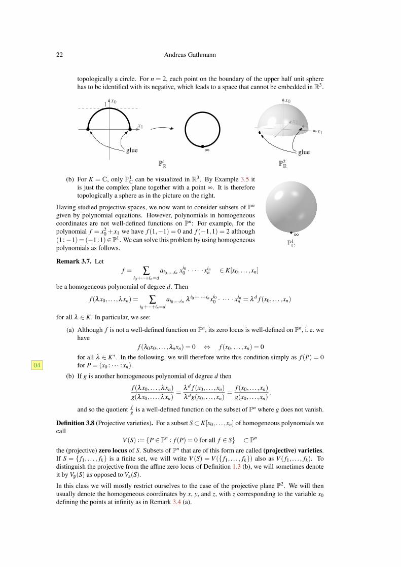
(b) For K = C, only P1C can be visualized in R3. By Example 3.5 it
is just the complex plane together with a point ∞. It is thereforetopologically a sphere as in the picture on the right.
Having studied projective spaces, we now want to consider subsets of Pn
given by polynomial equations. However, polynomials in homogeneouscoordinates are not well-defined functions on Pn: For example, for thepolynomial f = x2
0 + x1 we have f (1,−1) = 0 and f (−1,1) = 2 although(1:−1)= (−1:1)∈P1. We can solve this problem by using homogeneouspolynomials as follows.
∞
P1C
Remark 3.7. Letf = ∑
i0+···+in=dai0,...,in xi0
0 · · · · · xinn ∈ K[x0, . . . ,xn]
be a homogeneous polynomial of degree d. Then
f (λx0, . . . ,λxn) = ∑i0+···+in=d
ai0,...,in λi0+···+inxi0
0 · · · · · xinn = λ
d f (x0, . . . ,xn)
for all λ ∈ K. In particular, we see:
(a) Although f is not a well-defined function on Pn, its zero locus is well-defined on Pn, i. e. wehave
f (λ0x0, . . . ,λnxn) = 0 ⇔ f (x0, . . . ,xn) = 0
for all λ ∈ K∗. In the following, we will therefore write this condition simply as f (P) = 0for P = (x0 : · · · :xn).04
(b) If g is another homogeneous polynomial of degree d then
f (λx0, . . . ,λxn)
g(λx0, . . . ,λxn)=
λ d f (x0, . . . ,xn)
λ dg(x0, . . . ,xn)=
f (x0, . . . ,xn)
g(x0, . . . ,xn),
and so the quotient fg is a well-defined function on the subset of Pn where g does not vanish.
Definition 3.8 (Projective varieties). For a subset S⊂K[x0, . . . ,xn] of homogeneous polynomials wecall
V (S) := {P ∈ Pn : f (P) = 0 for all f ∈ S} ⊂ Pn
the (projective) zero locus of S. Subsets of Pn that are of this form are called (projective) varieties.If S = { f1, . . . , fk} is a finite set, we will write V (S) = V ({ f1, . . . , fk}) also as V ( f1, . . . , fk). Todistinguish the projective from the affine zero locus of Definition 1.3 (b), we will sometimes denoteit by Vp(S) as opposed to Va(S).
In this class we will mostly restrict ourselves to the case of the projective plane P2. We will thenusually denote the homogeneous coordinates by x, y, and z, with z corresponding to the variable x0defining the points at infinity as in Remark 3.4 (a).

3. Projective Curves 23
Remark 3.9. The properties of Remark 1.4 hold analogously for the projective zero locus: For anytwo homogeneous polynomials f ,g ∈ K[x,y,z] we have
(a) V ( f )∪V (g) =V ( f g);(b) V ( f )∩V (g) =V ( f ,g).
Exercise 3.10. By a projective coordinate transformation we mean a map f : Pn→ Pn of the form
(x0 : · · · :xn) 7→ ( f0(x0, . . . ,xn) : · · · : fn(x0, . . . ,xn))
for linearly independent homogeneous linear polynomials f0, . . . , fn ∈ K[x0, . . . ,xn].Now let P1, . . . ,Pn+2 ∈ Pn be points such that any n+1 of them are linearly independent in Kn+1, andin the same way let Q1, . . . ,Qn+2 ∈ Pn be points such that any n+1 of them are linearly independent.Show that there is a projective coordinate transformation f with f (Pi) = Qi for all i = 1, . . . ,n+2.
Exercise 3.11. Show:
(a) If F,G ∈ K[x0, . . . ,xn] are polynomials such that F |G and G is homogeneous, then F ishomogeneous.
(b) Every homogeneous polynomial in two variables over an algebraically closed field is a prod-uct of linear polynomials.
The definition of projective plane curves is now completely analogous to the affine case in Definition1.5.
Definition 3.12 (Projective curves).(a) A (projective plane algebraic) curve (over K) is a non-constant homogeneous polynomial
F ∈ K[x,y,z] modulo units. We call V (F) = {P ∈ P2 : F(P) = 0} its set of points.(b) The degree of a projective curve is its degree as a polynomial. As in the affine case, curves of
degree 1,2,3, . . . are called lines, quadrics/conics, cubics, and so on. The line z is referredto as the line at infinity.
(c) The notions of irreducible/reducible/reduced curves, as well as of irreducible componentsand their multiplicities, are defined in the same way as for affine curves in Definition 1.5(c) (note that irreducible factors of homogeneous polynomials are always homogeneous byExercise 3.11 (a)).
To study projective curves, we will often want to relate them to affine curves. For this we need thefollowing construction.
Construction 3.13 (Homogenization and dehomogenization).(a) For a polynomial
f = ∑i+ j≤d
ai, j xiy j ∈ K[x,y]
of degree d we define the homogenization of f as
f h := ∑i+ j≤d
ai, j xiy jzd−i− j ∈ K[x,y,z].
Note that f h is homogeneous of degree deg f h = deg f = d, and that z 6 | f h since f containsa term with i+ j = d.
(b) For a homogeneous polynomial
f = ∑i+ j+k=d
ai, j,k xiy jzk ∈ K[x,y,z]
of degree d we define the dehomogenization of f to be
f i := f (z = 1) = ∑i+ j+k=d
ai, j,k xiy j ∈ K[x,y].
In general, f i will be an inhomogeneous polynomial. If z 6 | f , i. e. if f contains a monomialwithout z, then this monomial will also be present in f i, and thus deg f i = deg f = d.

24 Andreas Gathmann
In particular, there is a bijective correspondence{polynomials of degree d
in K[x,y]
}←→
{homogeneous polynomials of degree d
in K[x,y,z] not divisible by z
}f 7−→ f h
f i ←−7 f .
Example 3.14. For f = y− x2 ∈ K[x,y] we have f h = yz− x2 ∈ K[x,y,z], and then back again( f h)i = y− x2 = f .
Remark 3.15 (Affine parts and projective closures).(a) For a projective curve F its affine set of points is Vp(F)∩A2 = Va(F(z = 1)) = Va(F i).
We will therefore call F i the affine part of F . The points at infinity of F are given byVp(F(z = 0))⊂ P1.
(b) For an affine curve F we call Fh its projective closure. By Construction 3.13 it is a pro-jective curve whose affine part is again F , and that does not contain the line at infinity as acomponent.
However, Fh may contain points at infinity: If F = F0 + · · ·+Fd is the decomposition intohomogeneous parts as in Notation 2.18, we have Fh = zd F0 + zd−1 F1 + · · ·+Fd and henceFh(z = 0) = Fd . So the points at infinity of F are given by the projective zero locus of theleading part of F .
Example 3.16 (Visualization of projective curves). To visualize a projective curve F , we will usuallyjust draw its affine set of points Va(F i), and if desired in addition its points at infinity as directions inA2. The following picture shows in this way the projective closures of the three types of real conics— a hyperbola, a parabola, and an ellipse (resp. a circle) — where the dashed lines correspond to thepoints at infinity. We see that the hyperbola has two points at infinity (namely (0:1 :0) and (1:0 :0)in the case below), the parabola has one ((0:1 :0) below), and the circle no such point. Note that,including these additional points, all three cases become topologically a loop, as the unboundedends of the affine curves meet up at the corresponding points at infinity. In fact, up to a change ofcoordinates, we will see in Exercise 3.28 that there is essentially only one type of real projectiveconic.
F = xy−1Fh = xy− z2
points at infinity: xy = 0
F = x2 + y2−1Fh = x2 + y2− z2
points at infinity: x2 + y2 = 0
F = y− x2
Fh = yz− x2
points at infinity: x2 = 0
(a) hyperbola (c) ellipse(b) parabola
Remark 3.17 (Spaces of curves as projective spaces). For d ∈ N>0, the vector space of homoge-neous polynomials of degree d in K[x,y,z] has dimension
(d+22
), hence it is isomorphic to Kn+1 with
n =(d+2
2
)− 1. By definition, a projective curve of degree d is then a non-zero point of this vector
space modulo scalars. Hence, the space of all such curves is just the projective space Pn, and thusitself a projective variety.
It is in fact very special to algebraic geometry — and very powerful — that the spaces of (certain)varieties are again varieties, and thus can be studied with exactly the same methods as the initialobjects themselves. In other categories this is usually far from being true: The space of all groups is

3. Projective Curves 25
not a group, the space of all vector spaces is not a vector space, the space of all topological spaces isnot a topological space, and so on.
For the rest of this chapter, let us transfer our results on affine curves from Chapters 1 and 2 to theprojective case.
Remark 3.18 (Recovering F from V (F)). Let F be a projective curve over an algebraically closedfield. We can write it as F = zm G for some m∈N and a curve G with z 6 | G. Then G can be recoveredfrom Gi since G = (Gi)h by Construction 3.13, and Gi can be recovered from Va(Gi) =Vp(G)∩A2
and a multiplicity on each component by Remark 1.14.
As the components of F are just the components of G plus possibly the line at infinity z (with multi-plicity m), this means that F can be reconstructed from V (F) and a multiplicity on each component,just as in the affine case.
Remark 3.19 (Finiteness of zero loci). Let F and G be two projective curves. The finiteness re-sults of Lemma 1.11 and Proposition 1.12 hold for the affine parts of F and G (for any choice ofcoordinate determining the line at infinity), and thus for F and G themselves: V (F) is infinite if Kis algebraically closed, P2\V (F) is infinite if K is infinite, and V (F,G) is finite if F and G have nocommon component.
Construction 3.20 (Local rings of P2). For P ∈ P2 we define the local ring of P2 at P according toRemark 3.7 (b) as
OP :=OP2,P :={
fg
: f ,g ∈ K[x,y,z] homogeneous of the same degree with g(P) 6= 0}⊂K(x,y,z).
As in Definition 2.1, these rings admit a well-defined evaluation map
OP→ K,fg7→ f (P)
g(P)with kernel
IP := IP2,P :={
fg∈ OP : f (P) = 0
}⊂OP.
For a point P = (x0 :y0 :1) in the affine part of P2 it is easily checked that there is an isomorphism
OP2,(x0 :y0 :1)→ OA2,(x0,y0),
fg7→ f i
gi
compatible with the evaluation maps, and thus taking IP2,(x0 :y0 :1) to IA2,(x0,y0). Hence the local rings
are still the same as in the affine case — which is of course expected, as objects that are local arounda point in A2 should not be affected by adding points at infinity.
Construction 3.21 (Intersection multiplicities). Note that the local ring OP2,P does not containK[x,y,z] as a subring. But for F1, . . . ,Fk homogeneous there is still a generated ideal
〈F1, . . . ,Fk 〉={
a1
b1F1 + · · ·+
ak
bkFk : ai,bi homogeneous with deg(aiFi) = degbi for all i
}in OP. As in the affine case we can therefore define the intersection multiplicity of two curves F,Gat a point P ∈ P2 as
µP(F,G) := dim OP/〈F,G〉 ∈ N∪{∞}. (∗)For a point P = (x0 :y0 :1) in the affine part of P2 one can verify directly that the isomor-phism OP2,(x0 :y0 :1)
∼= OA2,(x0,y0)of Construction 3.20 takes 〈F,G〉 to 〈F i,Gi 〉. Hence we have
µ(x0 :y0 :1)(F,G) = µ(x0,y0)(Fi,Gi), i. e. intersection multiplicities in the affine part can be computed
exactly as in Chapter 2. At other points, the multiplicity can be computed similarly by choosinganother (non-zero) coordinate to define the line at infinity as in Remark 3.4 (b). We will thereforeprobably never use the global definition (∗) of the multiplicity above for actual computations; itsonly purpose is to ensure that the result does not depend on the choice of coordinate defining the lineat infinity.

26 Andreas Gathmann
Moreover, in the same way as in Remark 2.4 (a) intersection multiplicities are invariant under pro-jective coordinate transformations as in Exercise 3.10, and they satisfy all the other properties of themultiplicities in Remark 2.4, Lemma 2.5, and Proposition 2.9.
Example 3.22. Let us compute the intersection multiplicity of the curveF = yz− x2 (whose affine part is shown on the right) with the line G = zat infinity at the common point P = (0:1 :0). For this we choose theaffine part given by y = 1 and affine coordinates x and z. We then obtain
µP(F,G) = µ(0,0)(z− x2,z) = 2
by Example 2.10.
F
Construction 3.23 (Tangents and multiplicities of points, smooth and singular points). The remain-ing concepts of Chapter 2 are also transferred easiest to a projective curve F using affine parts. Sofor a point P = (x0 :y0 :1) ∈ P2 in the affine part A2, we define the multiplicity mP(F) of F at Pto be m(x0,y0)(F
i) in the sense of Definition 2.20. A tangent to F at P is the projective closure of atangent to F i at (x0,y0). If P is not in the affine part, we choose a different coordinate for the line atinfinity as in Example 3.22.
We say that P ∈ F is a smooth or regular point if mP(F) = 1; its unique tangent is denoted TPF .Otherwise, P is called a singular point of F . The curve F is said to be smooth or regular if all itspoints are smooth; otherwise F is called singular.
As in the affine case, there is a simple criterion to determine all singular points of a given projectivecurve. To prove it, we need a simple lemma first.
Lemma 3.24. For any homogeneous polynomial F ∈ K[x,y,z] of degree d we have
x∂F∂x
+ y∂F∂y
+ z∂F∂ z
= d F.
Proof. For F = ∑i+ j+k=d ai, j,k xiy jzk we have x ∂F∂x = ∑i+ j+k=d iai, j,k xiy jzk. An analogous formula
holds for the other partial derivatives, and hence we conclude
x∂F∂x
+ y∂F∂y
+ z∂F∂ z
= ∑i+ j+k=d
(i+ j+ k)ai, j,k xiy jzk = d F. �
Proposition 3.25 (Projective Jacobi Criterion). Let P be a point on a projective curve F.
(a) P is a singular point of F if and only if ∂F∂x (P) =
∂F∂y (P) =
∂F∂ z (P) = 0.
(b) If P is a smooth point of F the tangent to F at P is given by
TPF =∂F∂x
(P) · x+ ∂F∂y
(P) · y+ ∂F∂ z
(P) · z.
Proof. Without loss of generality we may assume that P = (x0 :y0 :1) is in the affine part of F .
(a) By the affine Jacobi criterion of Proposition 2.26 (a) we know that P is a singular point ofF if and only if ∂F i
∂x (x0,y0) =∂F i
∂y (x0,y0) = 0. As dehomogenizing F (which is just settingz = 1) commutes with taking partial derivatives with respect to x and y, this is equivalent to∂F∂x (P) =
∂F∂y (P) = 0. This is in turn equivalent to ∂F
∂x (P) =∂F∂y (P) =
∂F∂ z (P) = 0 by Lemma
3.24 since F(P) = 0 by assumption.05

3. Projective Curves 27
(b) By Proposition 2.26 (b) the affine tangent to F at P is given by
∂F i
∂x(x0,y0) · (x− x0)+
∂F i
∂y(x0,y0) · (y− y0)
=∂F∂x
(P) · x+ ∂F∂y
(P) · y−(
∂F∂x
(P) · x0 +∂F∂y
(P) · y0
)3.24=
∂F∂x
(P) · x+ ∂F∂y
(P) · y+ ∂F∂ z
(P).
By definition, TPF is now obtained by taking the projective closure, i. e. the homogenizationof this polynomial. �
Remark 3.26. If the ground field K has characteristic 0, Lemma 3.24 tells us for any point P ∈ P2
that the conditions ∂F∂x (P) =
∂F∂y (P) =
∂F∂ z (P) = 0 already imply F(P) = 0. In contrast to the affine
case in Example 2.27, we therefore do not have to check explicitly that the point lies on the curvewhen computing singular points with the Jacobi criterion.
Example 3.27. Let F = y2z− x2z− x3 be the projective closure of thereal affine curve y2− x2− x3 of Example 2.23 (b). We have
∂F∂x
=−2xz−3x2,∂F∂y
= 2yz,∂F∂ z
= y2− x2.
It is checked immediately that the only common zero of these three poly-nomials is the point (0:0 :1), i. e. the origin of the affine part of F . So byProposition 3.25 this is the only singular point of F (note that we havealready seen in Example 2.27 using the affine Jacobi criterion that theorigin is the only singular point of the affine part of F).
F
In particular, the point (0:1 :0) ∈ F at infinity is a smooth point of F , and the tangent to F there isby Proposition 3.25
∂F∂x
(0:1 :0) · x+ ∂F∂y
(0:1 :0) · y+ ∂F∂ z
(0:1 :0) · z = z,
i. e. the line at infinity.
Exercise 3.28. Let F and G be two real smooth projective conics with non-empty set of points.Show that there is a projective coordinate transformation of P2 as in Exercise 3.10 that takes F to G.
Exercise 3.29. For a projective curve F in the homogeneous coordinates x0,x1,x2 we define theassociated Hessian to be HF := det( ∂ 2F
∂xi∂x j)i, j=0,1,2.
(a) Show that the Hessian is compatible with coordinate transformations, i. e. if a projectivecoordinate transformation as in Exercise 3.10 takes F to F ′ then it takes HF to HF ′ .
(b) Let P ∈ F be a smooth point, and assume that the characteristic of the ground field K is 0.Show that HF(P) = 0 if and only if µP(F,TPF)≥ 3. Such a point is called an inflection pointof F .
Hint: By part (a) and Exercise 3.10 you may assume after a coordinate transformation thatP = (0:0 :1) and TPF = x1.
28 Andreas Gathmann
4. Bézout’s Theorem
Let F and G be two projective curves without common component. We have seen already in Remark3.19 that the intersection F ∩G is finite in this case. Bézout’s Theorem, which is the main goal ofthis chapter, will determine the number of these intersection points, where each such point P will becounted with its intersection multiplicity µP(F,G).
In the same way as for the number of zeros of a univariate polynomial, the result will only be nice(i. e. depend only on the degree of the polynomials) if we assume that the underlying ground fieldis algebraically closed. To use this assumption we will need the following result from commutativealgebra that extends the defining property of an algebraically closed field to polynomials in severalvariables.
Fact 4.1 (Hilbert’s Nullstellensatz). Recall that a field K is called algebraically closed if everyunivariate polynomial f ∈ K[x] without a zero in K is constant.
An obvious generalization of this statement to the multivariate case (which can be proven easilyby induction of the number of variables) would be that every polynomial f ∈ K[x1, . . . ,xn] withouta zero in An is constant. However, there is a much stronger statement that also applies to severalpolynomials at once, or more precisely to the ideal generated by them: Any ideal I in K[x1, . . . ,xn]with V (I) = /0 over an algebraically closed field K is the unit ideal I = 〈1〉. This statement iscalled by its German name Hilbert’s Nullstellensatz (“theorem of the zeros”) [G6, Remark 10.12].Obviously, in the case n = 1 of polynomials in one variable, the ideal I must be generated by a singlepolynomial f as K[x1] is a principal ideal domain, and thus Hilbert’s Nullstellensatz just reduces tothe original statement that f must be constant if it does not have a zero.
Although Bézout’s Theorem requires projective curves (as we have already motivated at the begin-ning of Chapter 3), it is actually more convenient to perform almost all steps required in its proof forthe affine case. Our first step will be to compute the sum ∑P∈F∩G µP(F,G) of the local intersectionmultiplicities of two affine curves F and G and express it in terms of one global object. In fact, in thesame way as µP(F,G) is by definition the dimension of the quotient of the local ring OP by the ideal〈F,G〉, the sum of these multiplicities is just the dimension of the quotient of the global polynomialring K[x,y] by 〈F,G〉:
Lemma 4.2. Let F and G be two affine curves over K with no common component. We consider thenatural ring homomorphism
ϕ : K[x,y]/〈F,G〉 → ∏P∈F∩G
OP/〈F,G〉
that sends the class of a polynomial f ∈ K[x,y] to the class of f ∈ OP in each factor OP/〈F,G〉.
(a) The morphism ϕ is surjective.
(b) If K is algebraically closed then ϕ is an isomorphism.
In particular, we have ∑P µP(F,G)≤ dimK[x,y]/〈F,G〉, with equality if K is algebraically closed.
Proof.
(a) Let F ∩G = {P0, . . . ,Pm}. We show the surjectivity of ϕ in three steps, each producingpolynomials with increasingly general images under ϕ .
Step 1: If Pi = (xi,yi) for i = 0, . . . ,m, and we set
f := ∏i:xi 6=x0
(x− xi) · ∏i:yi 6=y0
(y− yi) ∈ K[x,y],

4. Bézout’s Theorem 29
then by construction f (P0) 6= 0, and f (Pi) = 0 for all i > 0.
Step 2: Now choose n > µPi(F,G) for all i; we claim that the polynomial f of Step 1 satisfiesf n = 0 in OPi/〈F,G〉 for all i > 0. In fact, the chain of ideals
〈F,G, f 0 〉 ⊃ 〈F,G, f 1 〉 ⊃ · · · ⊃ 〈F,G, f n 〉
in OPi leads to a chain of inequalities
dimOPi/〈F,G, f 0 〉 ≤ dimOPi/〈F,G, f 1 〉 ≤ · · · ≤ dimOPi/〈F,G, f n 〉.
But all of these numbers are at most dimOPi/〈F,G〉 and thus less than n. Hence, we musthave equality at some stage, i. e. 〈F,G, f k 〉= 〈F,G, f k+1 〉 in OPi for some k ∈ {0, . . . ,n−1}(depending on i). This means that f k = aF + bG+ c f k+1 for some a,b,c ∈ OPi , and thusf k(1− c f ) ∈ 〈F,G〉. But 1− c f has value 1 at Pi and hence is a unit in OPi . We concludethat f k ∈ 〈F,G〉 in OPi , which implies f n = 0 ∈ OPi/〈F,G〉 for all i > 0 as desired.
Step 3: Finally, let a ∈ OP0 be arbitrary. By Exercise 2.17 (b) we know that af n has a poly-
nomial representative g in OP0 . Then the morphism ϕ maps g f n to af n · f n = a in the first
factor OP0/〈F,G〉, and to 0 in all other factors since f n = 0 there. Hence all elements of∏P∈F∩G OP/〈F,G〉 with arbitrary entry in the P0-component and zero entries in all othercomponents lie in the image of ϕ . By symmetry, the same holds for all other points Pi, andas the image of ϕ must be a subring we conclude that ϕ is surjective.
(b) In view of (a) it remains to be shown that f is injective. So let f ∈ kerϕ , and consider theset I := {g∈K[x,y] : g f ∈ 〈F,G〉}. This is clearly an ideal containing 〈F,G〉 (usually calledthe ideal quotient 〈F,G〉 : 〈 f 〉). By the Nullstellensatz of Fact 4.1 it suffices to prove thatV (I) = /0, since then I =K[x,y], hence 1∈ I, i. e. f ∈ 〈F,G〉, and thus f = 0∈K[x,y]/〈F,G〉.So assume that there is a point P∈V (I). As F,G∈ I we know that P∈ F∩G. Hence P is oneof the points in the product in the target space of ϕ , and so f = 0 ∈OP/〈F,G〉 as f ∈ kerϕ .This means that f = a
g F + bg G for some polynomials a,b,g ∈ K[x,y] with g(P) 6= 0. But then
g f = aF +bG, hence g ∈ I, and as P ∈V (I) we arrive at the contradiction g(P) = 0. �
Remark 4.3. There are two ways to interpret the statement of Lemma 4.2:
(a) A case that often occurs in Lemma 4.2 is that F and G intersect transversely, i. e. that theintersection multiplicities µP(F,G) at all P ∈ F ∩G are equal to 1. In this case every factorOP/〈F,G〉 is isomorphic to K by Definition 2.3, and the morphism ϕ is just the combinedevaluation map at all points of F ∩G. The assertion of Lemma 4.2 (a) is then simply the in-terpolation statement that we can always find a polynomial having prescribed values at thesepoints — which is probably not surprising, and is in fact already achieved by a suitable linearcombination of polynomials as in Step 1 in the proof. If the intersection is not transverseand µP(F,G)> 1 at some point P, then the map ϕ remembers more information at P on thepolynomial than just its value, such as the values of some of its partial derivatives at P.
(b) If you have some commutative algebra background then you probably know the statementof Lemma 4.2 already: As V (F,G) is 0-dimensional, the ring K[x,y]/〈F,G〉 is Artinian,and thus by the Structure Theorem on Artinian rings it is isomorphic to the product of itslocalizations at its various maximal ideals [G6, Proposition 7.20]. If K is algebraically closedthen these maximal ideals all correspond to points in A2 [G6, Corollary 10.10], and so themap ϕ of the lemma is an isomorphism. If K is not necessarily algebraically closed thenthere are maximal ideals of K[x,y]/〈F,G〉 that are not of this form and thus “missing” in thetarget space of ϕ , so that ϕ is only surjective.
Of course, our goal must now be to compute the dimension of the quotient K[x,y]/〈F,G〉. In orderto do this, we need a lemma first that tells us how polynomials in the ideal 〈F,G〉 of K[x,y] can berepresented.

30 Andreas Gathmann
Lemma 4.4. Let F and G be two affine curves of degrees m := degF and n := degG, respectively,such that their leading parts Fm and Gn (as in Notation 2.18) have no common component.
Then every f ∈ 〈F,G〉 ⊂ K[x,y] of degree d := deg f can be written as f = aF +bG for two polyno-mials a and b with dega≤ d−m and degb≤ d−n.
Proof. As f ∈ 〈F,G〉we can write f = aF+bG for some a,b∈K[x,y]; choose such a representationwith dega minimal.
Assume for a contradiction that dega > d−m or degb > d−n. Then aF or bG contains a term ofdegree bigger than d. As f = aF + bG has degree d this means that the leading terms of aF andbG must cancel in f . Hence, if a∗ and b∗ denote the leading terms of a and b, respectively, we havea∗Fm = −b∗Gn. But Fm and Gn have no common component by assumption, and so we must havea∗ = cGn and b∗ =−cFm for some homogeneous polynomial c. This gives us a new representation
f = (a− cG)F +(b+ cF)G
in which the leading term a∗ of a cancels the leading term cGn of cG in the first bracket. Hencedeg(a− cG)< dega, contradicting the minimality of dega. �
Lemma 4.5. Let F and G be affine curves with no common component, of degrees m := degF andn := degG.
(a) dimK[x,y]/〈F,G〉 ≤ mn.
(b) If the leading parts Fm and Gn have no common component either then equality holds in (a).
Proof.
(a) For all d ≥ m+n consider the sequence of vector space homomorphisms
K[x,y]≤d−m×K[x,y]≤d−nα−→ K[x,y]≤d
π−→ K[x,y]/〈F,G〉
(a,b) 7−→ aF +bG
where K[x,y]≤d denotes the vector subspace of K[x,y] of all polynomials of degree at mostd, which has dimension
(d+22
), and π is the quotient map.
The kernel of α consists of all pairs (a,b) of polynomials of degrees at most d−m and d−n,respectively, with aF = −bG. As F and G have no common component, this is equivalentto a = cG and b =−cF for some c ∈ K[x,y]≤d−m−n, so that
kerα = K[x,y]≤d−m−n · (G,−F). (1)
Moreover, it is obvious that
imα ⊂ kerπ. (2)06
So we conclude with the homomorphism theorem
dimimπ =
(d +2
2
)−dimkerπ
(2)≤(
d +22
)−dimimα
=
(d +2
2
)−(
d−m+22
)−(
d−n+22
)+dimkerα
(1)=
(d +2
2
)−(
d−m+22
)−(
d−n+22
)+
(d−m−n+2
2
)= mn.
Note that this bound is independent of d (as long as d ≥ m+n), and thus also holds for theprojection map π : K[x,y]→ K[x,y]/〈F,G〉 from the full polynomial ring, which is surjec-tive. It follows that dimK[x,y]/〈F,G〉 ≤ mn.

4. Bézout’s Theorem 31
(b) It suffices to establish equality in (2) in the proof of (a) above, i. e. that kerπ ⊂ imα . Butthis is precisely the statement of Lemma 4.4. �
We can now switch back to the projective case and prove the main result of this chapter.
Corollary 4.6 (Bézout’s Theorem). Let F and G be projective curves without common componentover an infinite field K. Then
∑P∈F∩G
µP(F,G)≤ degF ·degG.
Moreover, equality holds if K is algebraically closed.
Proof. By Lemma 1.11 (b) there is a point Q in the affine part of P2 which does not lie on F i∪Gi,i. e. neither on F nor on G. Moreover, as K is infinite but F ∩G finite by Proposition 1.12, wecan pick a line L through Q which does not intersect F ∩G. Now we make a projective coordinatetransformation so that L becomes the line at infinity. Then neither F nor G contains the line at infinityas a component (so that degF i = degF and degGi = degG), and all intersection points of F and Glie in the affine part (i. e. they are also intersection points of the affine curves F i and Gi).
Applying Lemma 4.2 (a) and 4.5 (a) to F i and Gi then yields
∑P∈F∩G
µP(F,G) = ∑P∈F i∩Gi
µP(F i,Gi)4.2≤ dimK[x,y]/〈F i,Gi 〉
4.5≤ degF i ·degGi = degF ·degG. (∗)
Now let K be algebraically closed. Then the first inequality is actually an equality by Lemma 4.2(b). Moreover, the leading parts of F i and Gi are homogeneous polynomials in two variables, andhence a product of linear factors by Exercise 3.11 (b). But these factors correspond exactly to thepoints at infinity of the two curves by Remark 3.15 (b). As there are no such common points by ourchoice of L, we conclude that the leading parts of F i and Gi have no common component, and thusby Lemma 4.5 (b) that the second inequality in (∗) is actually an equality as well. �
Remark 4.7 (Bézout’s Theorem over arbitrary ground fields). It can be shown that (the inequalitypart of) Bézout’s Theorem holds in fact over arbitrary fields. The assumption of an infinite groundfield was only necessary for the strategy of our proof to choose coordinates so that all intersectionpoints of the curves lie in the affine part — which would not be possible over finite fields, since thetwo curves might then intersect in every point of P2 (without having a common component).
Remark 4.8. Let F and G be two projective curves without common component over an infiniteground field K.
(a) As the intersection multiplicity at each point of F ∩G is at least 1, it follows from Bézout’sTheorem that F and G intersect in at most degF ·degG points (disregarding the multiplici-ties).
(b) If K is algebraically closed, Bézout’s Theorem implies in particular that F and G intersectin at least one point. Note that already this statement is non-trivial — and clearly false forgeneral ground fields, as then already V (F) might be empty.
Exercise 4.9. For the following complex affine curves F and G, determine the points at infinity oftheir projective closures, and use Bézout’s Theorem to read off the intersection multiplicities at allpoints of F ∩G.
(a) F = x+ y2 and G = x+ y2− x3;
(b) F = y2− x2 +1 and G = (y+ x+1)(y− x+1).
Exercise 4.10. Deduce the following real version of Bézout’s Theorem from the complex case: If Fand G are two real projective curves without common components then
∑P∈F∩G
µP(F,G) = degF ·degG mod 2.
In particular, two real projective curves of odd degree always intersect in at least one point.

32 Andreas Gathmann
Exercise 4.11. Let F be a complex irreducible projective curve of degree d, and let P ∈ P2 be apoint. We set m := mP(F) ∈ N.
Show that for all but finitely many lines L in P2 through P, the intersection F ∩L consists of exactlyd−m points not equal to P.
We will discuss many examples and applications of Bézout’s Theorem in the next chapter. Instead,at the end of this chapter let us prove another theorem that can be obtained by very similar methodsand that will be useful later on. It considers a smooth projective curve F over an algebraically closedfield and states roughly that, for any two other curves G and H such that F intersects H everywherewith at least the same multiplicity as G, the “remaining multiplicities” µP(F,H)− µP(F,G) can beobtained by intersecting F with another curve.
Corollary 4.12 (Noether’s Theorem). Let F be a smooth projective curve over an algebraicallyclosed field. Moreover, let G and H be two projective curves that do not have a common componentwith F.
If µP(F,G) ≤ µP(F,H) for all points P ∈ P2 then there are homogeneous polynomials A and B (ofdegrees degH−degF resp. degH−degG if non-zero), such that
(a) H = AF +BG;
(b) µP(F,H) = µP(F,G)+µP(F,B) for all P ∈ P2.
Proof. As in the proof of Corollary 4.6 we may assume by a projective coordinate transformationthat none of the curves contain the line at infinity as a component, and that all points of F ∩G lie inthe affine part of P2. We then have again degF i = degF , degGi = degG, degH i = degH, and theleading parts of F i and Gi have no common component.
Now F is assumed to be smooth, and hence — working with the affine curves for a moment —the assumption µP(F i,Gi) ≤ µP(F i,H i) implies 〈F i,H i 〉 ⊂ 〈F i,Gi 〉 in OP for all P ∈ F ∩G byProposition 2.28, and thus in particular H i ∈ 〈F i,Gi 〉 in OP. By Lemma 4.2 (b) we then haveH i ∈ 〈F i,Gi 〉 in K[x,y] as well. But as the leading parts of F i and Gi have no common component,Lemma 4.4 gives us an equation
H i = aF i +bGi
for some polynomials a and b of degrees at most degH − degF and degH − degG, respectively.Homogenizing this yields H, so a homogeneous polynomial of degree degH, and thus
H = zdegH−degF−degaah︸ ︷︷ ︸=:A
F + zdegH−degG−degbbh︸ ︷︷ ︸=:B
G,
which proves (a). But this also implies part (b), since by (the projective version of) the properties ofintersection multiplicities we have
µP(F,H) = µP(F,AF +BG)2.4 (c)= µP(F,BG)
2.9 (b)= µP(F,B)+µP(F,G). �
Exercise 4.13 (Cayley-Bacharach ). Let F and G be smooth projective cubics over an algebraicallyclosed field that intersect in exactly 9 points P1, . . . ,P9. Moreover, let E be another cubic that alsocontains the first eight points P1, . . . ,P8. Prove that E then also contains P9.
(Hint: Apply Noether’s Theorem to a suitable curve H.)
Exercise 4.14. Show by example that Noether’s Theorem is in general false . . .
(a) if the ground field is not algebraically closed; or
(b) if the curve F is not assumed to be smooth.
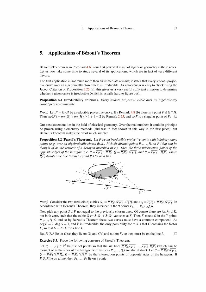
5. Applications of Bézout’s Theorem 33
5. Applications of Bézout’s Theorem
Bézout’s Theorem as in Corollary 4.6 is our first powerful result of algebraic geometry in these notes.Let us now take some time to study several of its applications, which are in fact of very differentflavors.
The first application is not much more than an immediate remark; it states that every smooth projec-tive curve over an algebraically closed field is irreducible. As smoothness is easy to check using theJacobi Criterion of Proposition 3.25 (a), this gives us a very useful sufficient criterion to determinewhether a given curve is irreducible (which is usually hard to figure out).
Proposition 5.1 (Irreducibility criterion). Every smooth projective curve over an algebraicallyclosed field is irreducible.
Proof. Let F = G ·H be a reducible projective curve. By Remark 4.8 (b) there is a point P ∈G∩H.Then mP(F) = mP(G)+mP(H)≥ 1+1 = 2 by Remark 2.25, and so P is a singular point of F . �
Our next statement lies in the field of classical geometry. Over the real numbers it could in principlebe proven using elementary methods (and was in fact shown in this way in the first place), butBézout’s Theorem makes the proof much simpler.
Proposition 5.2 (Pascal’s Theorem). Let F be an irreducible projective conic with infinitely manypoints (e. g. over an algebraically closed field). Pick six distinct points P1, . . . ,P6 on F (that can bethought of as the vertices of a hexagon inscribed in F). Then the three intersection points of theopposite edges of the hexagon (i. e. P = P1P2 ∩P4P5, Q = P2P3 ∩P5P6, and R = P3P4 ∩P6P1, wherePiPj denotes the line through Pi and Pj) lie on a line.
P3
P4
P1
P2
P5P6
PR
Q
F
Proof. Consider the two (reducible) cubics G1 = P1P2∪P3P4∪P5P6 and G2 = P2P3∪P4P5∪P6P1. Inaccordance with Bézout’s Theorem, they intersect in the 9 points P1, . . . ,P6,P,Q,R.
Now pick any point S ∈ F not equal to the previously chosen ones. Of course there are λ1,λ2 ∈ K,not both zero, such that the cubic G := λ1G1 +λ2G2 vanishes at S. Then F meets G in the 7 pointsP1, . . . ,P6,S, and so by Bézout’s Theorem these two curves must have a common component. AsdegF = 2, degG = 3, and F is irreducible, the only possibility for this is that G contains the factorF , so that G = F ·L for a line L.
But P,Q,R lie on G (as they lie on G1 and G2) and not on F , so they must be on the line L. �
Exercise 5.3. Prove the following converse of Pascal’s Theorem:
Let P1, . . . ,P6 ∈ P2 be distinct points so that the six lines P1P2,P2P3, . . . ,P5P6,P6P1 (which can bethought of as the sides of the hexagon with vertices P1, . . . ,P6) are also distinct. Let P = P1P2∩P4P5,Q = P2P3 ∩P5P6, R = P3P4 ∩P6P1 be the intersection points of opposite sides of the hexagon. IfP,Q,R lie on a line, then P1, . . . ,P6 lie on a conic.

34 Andreas Gathmann
Let us next address the question how many singular points we can have on a given projective curve.Exercise 2.32 (b) implies that, for an irreducible curve (over a field of characteristic 0), the numberof singular points is always finite. Using Bézout’s Theorem, we can now also give an upper boundfor this number.
Example 5.4 (Singular points in degrees 1 and 2). Let F be an irreducible projective curve withinfinitely many points (e. g. over an algebraically closed field).
(a) If degF = 1 then F is a line, which never has any singular points.
(b) If degF = 2 we claim that F has again no singular points. To show this, assume to thecontrary that P ∈ F is a singular point, and choose any other point Q ∈ F . Let G be the linethrough P and Q.
As P is a singular point of F , we know by Corollary 2.24 that µP(F,G)≥ 2. Hence the totalintersection multiplicity of F and G is at least
µP(F,G)+µQ(F,G)≥ 2+1 = 3,
which is bigger than degF · degG = 2. So by Bézout’s Theorem F and G must have acommon component — which is impossible since F and G are irreducible.
In fact, this argument is already the idea to find a bound for the number of singular points of a curveF of general degree: Find a suitable curve G through the assumed singular points and some otherpoints of F , and compute the total intersection multiplicity of F and G, where each singular point ofF can be counted with multiplicity at least 2. If this total number exceeds degF ·degG we arrive ata contradiction, i. e. the assumed number of singular points was too high.
In order to make this idea into an exact proof, we need an auxiliary lemma first that tells us how wecan find curves (such as G above) through a given number of points.
Lemma 5.5 (Curves through given points). Let d ∈N>0. For any(d+2
2
)−1 given points in P2 there
is a projective curve of degree d passing through them.
Proof. By Remark 3.17, the space of all projective curves of degree d is P(K[x,y,z]d), whereK[x,y,z]d denotes the vector space of all homogeneous polynomials of degree d over K. AsdimK[x,y,z]d =
(d+22
), we see that this is a projective space of dimension
(d+22
)− 1. In this space
P(d+2
2 )−1, a curve F = ∑i+ j+z=d ai, j,kxiy jzk corresponds to the point with homogeneous coordinatesai, j,k.
Now note that, for a given point P = (x0 :y0 :z0), the condition that P ∈ F translates to the equation∑i+ j+k=d ai, j,kxi
0y j0zk
0 = 0, i. e. to a linear condition in these homogeneous coordinates. The spaceof all projective curves of degree d passing through
(d+22
)−1 given points is therefore a projective
subspace of dimension at least dimP(d+2
2 )−1−((d+2
2
)−1)= 0, and thus non-empty. �
07Proposition 5.6. Let F be an irreducible projective curve of degree d with infinitely many points(e. g. over an algebraically closed field). Then F has at most
(d−12
)singular points.
Proof. By Example 5.4 it suffices to prove the proposition for curves ofdegree d ≥ 3. Assume for a contradiction that there are distinct singu-lar points P1, . . . ,P(d−1
2 )+1 of F . Moreover, pick d− 3 arbitrary furtherdistinct points Q1, . . . ,Qd−3 on F , so that the total number of points is(
d−12
)+1+d−3 =
(d2
)−1.
FG
P2
P1
Q1
By Lemma 5.5, there is therefore a curve G of degree d − 2 through all these points. As F isirreducible and of bigger degree than G, the curves F and G cannot have a common component.Hence Corollary 4.6 shows that F and G can intersect in at most degF · degG = d(d− 2) points,
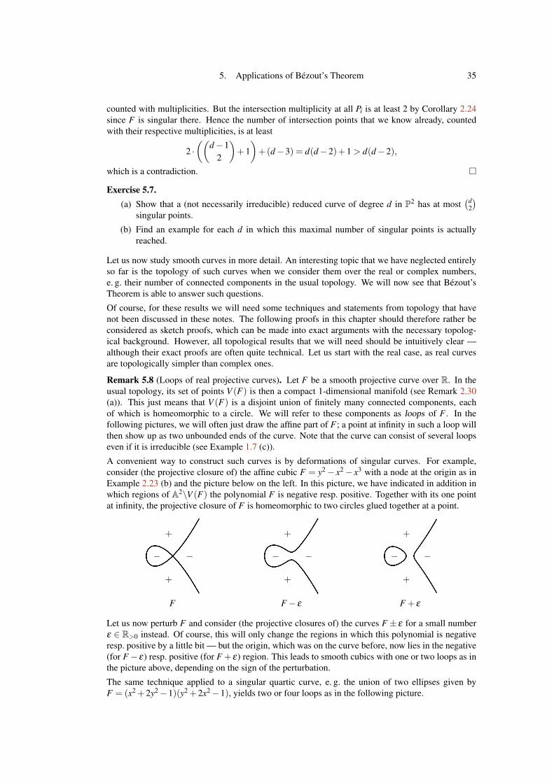
5. Applications of Bézout’s Theorem 35
counted with multiplicities. But the intersection multiplicity at all Pi is at least 2 by Corollary 2.24since F is singular there. Hence the number of intersection points that we know already, countedwith their respective multiplicities, is at least
2 ·((
d−12
)+1)+(d−3) = d(d−2)+1 > d(d−2),
which is a contradiction. �
Exercise 5.7.(a) Show that a (not necessarily irreducible) reduced curve of degree d in P2 has at most
(d2
)singular points.
(b) Find an example for each d in which this maximal number of singular points is actuallyreached.
Let us now study smooth curves in more detail. An interesting topic that we have neglected entirelyso far is the topology of such curves when we consider them over the real or complex numbers,e. g. their number of connected components in the usual topology. We will now see that Bézout’sTheorem is able to answer such questions.
Of course, for these results we will need some techniques and statements from topology that havenot been discussed in these notes. The following proofs in this chapter should therefore rather beconsidered as sketch proofs, which can be made into exact arguments with the necessary topolog-ical background. However, all topological results that we will need should be intuitively clear —although their exact proofs are often quite technical. Let us start with the real case, as real curvesare topologically simpler than complex ones.
Remark 5.8 (Loops of real projective curves). Let F be a smooth projective curve over R. In theusual topology, its set of points V (F) is then a compact 1-dimensional manifold (see Remark 2.30(a)). This just means that V (F) is a disjoint union of finitely many connected components, eachof which is homeomorphic to a circle. We will refer to these components as loops of F . In thefollowing pictures, we will often just draw the affine part of F ; a point at infinity in such a loop willthen show up as two unbounded ends of the curve. Note that the curve can consist of several loopseven if it is irreducible (see Example 1.7 (c)).
A convenient way to construct such curves is by deformations of singular curves. For example,consider (the projective closure of) the affine cubic F = y2− x2− x3 with a node at the origin as inExample 2.23 (b) and the picture below on the left. In this picture, we have indicated in addition inwhich regions of A2\V (F) the polynomial F is negative resp. positive. Together with its one pointat infinity, the projective closure of F is homeomorphic to two circles glued together at a point.
F F− ε F + ε
−
+
+
− −
+
+
− −
+
+
−
Let us now perturb F and consider (the projective closures of) the curves F± ε for a small numberε ∈ R>0 instead. Of course, this will only change the regions in which this polynomial is negativeresp. positive by a little bit — but the origin, which was on the curve before, now lies in the negative(for F−ε) resp. positive (for F +ε) region. This leads to smooth cubics with one or two loops as inthe picture above, depending on the sign of the perturbation.
The same technique applied to a singular quartic curve, e. g. the union of two ellipses given byF = (x2 +2y2−1)(y2 +2x2−1), yields two or four loops as in the following picture.

36 Andreas Gathmann
F F− ε F + ε
+
+
−−
−
−
+
+
−−
−
−
+
+
−−
−
−
Remark 5.9 (Even and odd loops). Although all loops of real smooth curves are homeomorphic to acircle, there are two different kinds of them when we consider their embeddings in projective space.To understand this, recall from Remark 3.6 (a) that P2
R is obtained from the upper half sphere (whichwe will draw topologically as an disc below) by identifying opposite points on the boundary, as inthe following picture on the left.
P2R P2
R P2R
identify Odd loopEven loop
P P
Q
P
P
Q
The consequence of this is that we have two different types of loops. An even loop is a loop such thatits complement has two connected components, which we might call its “interior” (shown in darkin the picture above, homeomorphic to a disc) and “exterior” (homeomorphic to a Möbius strip),respectively. In contrast, an odd loop does not divide P2
R into two regions; its complement is a singlecomponent homeomorphic to a disc. Note that the distinction between even and odd is not whetherthe affine part of the curve is bounded: Whereas an odd loop always has to be unbounded, an evenloop may well be unbounded, too. Instead, if you know some topology you will probably recognizethat the statement being made here is just that the fundamental group π1(P2
R) is isomorphic to Z/2Z;the two types of loops simply correspond to the two elements of this group.
In principle, a real curve can have even as well as odd loops. There is one restriction however: Asthe complement of an odd loop is simply a disc, all other loops in this complement will have aninterior and exterior, so that they are even. In other words, a real smooth curve can have at most oneodd loop.
We are now ready to find a bound on the number of loops in an irreducible smooth curve in P2R
of a given degree. Interestingly, the idea in its proof is almost identical to that of Proposition 5.6,although the resulting statement is quite different.
Proposition 5.10 (Harnack’s Theorem). An irreducible smooth curve of degree d in P2R has at
most(d−1
2
)+1 loops.
Example 5.11. A line (d = 1) has always exactly one loop. An irreducible smooth conic (d = 2) isa hyperbola, parabola, or ellipse as in Example 3.16, so in every case the number of loops is again1 (after adding the points at infinity). For d = 3 Harnack’s Theorem gives a maximum number of 2loops, and for d = 4 we get at most 4 loops. We have just seen examples of these numbers of loopsin Remark 5.8. In fact, one can show that the bound given in Harnack’s theorem is sharp, i. e. thatfor every d one can find real smooth curves of degree d with exactly
(d−12
)+1 loops.

5. Applications of Bézout’s Theorem 37
Proof sketch of Proposition 5.10. Let F be a real irreducible smoothprojective curve of degree d; by Example 5.11 it suffices to considerthe case d ≥ 3. Assume that the statement of the proposition is false,i. e. that there are at least
(d−12
)+ 2 loops. We have seen in Remark 5.9
that at least(d−1
2
)+ 1 of these loops must be even. Hence we can pick
points P1, . . . ,P(d−12 )+1 on distinct even loops of F , and d−3 more points
Q1, . . . ,Qd−3 on another loop (which might be even or odd). So, as in theproof of Proposition 5.6, we have a total of
(d2
)−1 points.
FGP1
P̃1
P̃2
P2 Q1
Again as in the proof of Proposition 5.6, it now follows that there is a real curve G of degree atmost d−2 passing through all these points. As F is irreducible and has bigger degree than G, thesetwo curves cannot have a common component, so Bézout’s Theorem as in Corollary 4.6 implies thatthey intersect in at most d(d− 2) points, counted with multiplicities. But recall from Remark 5.9that the even loops of F containing the points Pi divide the real projective plane into two regions,hence if G enters the interior of such a loop it has to exit it again at another point P̃i of the same loopas in the picture above (it may also happen that G is singular or tangent to F at Pi, in which caseµPi(F,G) ≥ 2 by Corollary 2.24). So in any case the total number of intersection points, countedwith their respective multiplicities, is at least
2 ·((
d−12
)+1)+(d−3) = d(d−2)+1 > d(d−2),
which is a contradiction. �
Let us now turn to the case of complex curves. Of course, their topology is entirely different, as theyare 2-dimensional spaces and thus surfaces in the usual topology. In fact, we have seen such a casealready in Example 0.2 of the introduction.
Remark 5.12 (Topology of complex curves). Let F be a smooth projective curve over C. Similarlyto the real case, its set of points V (F) is then a compact 1-dimensional complex manifold, and hencea 2-dimensional real manifold. Moreover, one can show:
(a) V (F) is always an oriented manifold, i. e. a “two-sided surface”, as opposed to e. g. a Möbiusstrip. To see this, note that all tangents TPF for P ∈ F are 1-dimensional complex vectorspaces after shifting P to the origin, and hence admit a well-defined multiplication with theimaginary unit i. Geometrically, this means that all tangent planes to the surface have a well-defined notion of a positive rotation by 90 degrees, varying continuously with P — whichdefines an orientation of the surface.
(b) In contrast to the real case that we have just studied, V (F) is always connected. In short,the reason for this is that the notion of degree as well as Bézout’s Theorem can be extendedto compact oriented 2-dimensional submanifolds of P2
C. Hence, if V (F) had (at least) twoconnected components X1 and X2, each of them would be a compact oriented 2-dimensionalmanifold itself, and there would thus be well-defined degrees degX1,degX2 ∈ N>0. Butthen X1 and X2 would have to intersect in degX1 ·degX2 points (counted with multiplicities),which is obviously a contradiction.
Of course, the methods needed to prove Bézout’s Theorem in the topological setting areentirely different from ours in Chapter 4. If you know some algebraic topology, the statementhere is that the 2-dimensional homology group H2(P2
C,Z) is isomorphic to Z. With thisisomorphism, the class of a compact oriented 2-dimensional submanifold in H2(P2
C,Z) isa positive number, and the intersection product H2(P2
C,Z)×H2(P2C,Z)→ H0(P2
C,Z) ∼= Z(using Poincaré duality) is just the product of these numbers.

38 Andreas Gathmann
It is now a (non-trivial but intuitive) topological result that a con-nected compact orientable 2-dimensional manifold X is alwayshomeomorphic to a sphere with some finite number of “handles”.This number of handles is called the (topological) genus of X .Hence every curve in P2
C can be assigned a genus that describes itstopological type. The picture on the right shows a complex curveof genus 2.
We will see in Definition 8.10 that there is also an algebraic way to assign a genus to a smoothprojective curve. It is then applicable to any (algebraically closed) ground field, coincides with thetopological genus over C and plays an important role in the study of functions on the curve. Ourgoal for the rest of this chapter however will just be to compute the topological genus of a smoothcomplex projective curve in terms of its degree. To do this, we will need the following techniquefrom topology.
Construction 5.13 (Cell decompositions). Let X be a compact 2-dimensional manifold. A celldecomposition of X is given by writing X topologically as a finite disjoint union of points, (open)lines, and (open) discs. This decomposition should be “nice” in a certain sense, e. g. the boundarypoints of every line in the decomposition must be points of the decomposition. We do not want togive a precise definition here (which would necessarily be technical), but only remark that every“reasonable” decomposition that one could think of will be allowed. For example, the followingpicture shows three valid decompositions of the complex curve P1
C, which is topologically a sphereby Remark 3.6 (b).
In the left two pictures, we have 1 point, 1 line, and 2 discs (the two halves of the sphere), whereasin the picture on the right we have 2 points, 4 lines, and 4 discs.
Of course, there are many possibilities for cell decompositions of X . But there is an importantnumber that does not depend on the chosen decomposition:
Lemma and Definition 5.14 (Euler characteristic). Let X be a compact 2-dimensional manifold.Consider a cell decomposition of X, consisting of σ0 points, σ1 lines, and σ2 discs. Then the number
χ := σ0−σ1 +σ2
depends only on X, and not on the chosen decomposition. We call it the (topological) Euler charac-teristic of X.
Proof sketch. Let us first consider the case when we move from one decomposition to a finer one,i. e. if we add points or lines to the decomposition. Such a process is always obtained by performingthe following steps a finite number of times:
• Adding another point on a line: In this case we raise σ0 and σ1 by 1 as in the picture below,hence the alternating sum χ = σ0−σ1 +σ2 does not change.
• Adding another line in a disc: In this case we raise σ1 and σ2 by 1, so again χ remainsinvariant.

5. Applications of Bézout’s Theorem 39
add apoint
add aline
We conclude that the alternating sum σ0−σ1 +σ2 does not change under refinements. But any twodecompositions have a common refinement — which is essentially given by taking all the points andlines in both decompositions, and maybe adding more points where two such lines intersect. Forexample, in Construction 5.13 the decomposition in the picture on the right is a common refinementof the other two. Hence the Euler characteristic is independent of the chosen decomposition. �
Example 5.15 (Euler characteristic ↔ genus). Let X bea connected compact orientable 2-dimensional manifold ofgenus g, and consider the cell decomposition of X as shownon the right. It has σ0 = 2g+2 points, σ1 = 4g+4 lines, and4 discs, and hence we conclude that the Euler characteristicof X is
χ = σ0−σ1 +σ2 = 2−2g.
In other words, the genus is given in terms of the Euler characteristic as g = 1− χ
2 .
We are now ready to compute the genus of a smooth curve in P2C.
Proposition 5.16 (Topological degree-genus formula). A smooth curve of degree d in P2C has
topological genus(d−1
2
).
08
Proof sketch. Let F be a smooth curve of degree d in P2C. By a projective coordinate transformation
we can assume that (0:1 :0) /∈ F . Then
π : V (F)→ P1C, (x :y :z) 7→ (x :z)
is a well-defined map that can be interpreted as a projection,since in the affine part where z = 1 it is given by (x,y) 7→ x as inthe picture on the right. Let us study its inverse images of a fixedpoint (x :z) ∈ P1
C. Of course, they are given by the values of ysuch that F(x,y,z) = 0, so that there are exactly d such points— unless the polynomial F(x, · ,z) has a multiple zero in y at apoint in the inverse image, which happens if and only if F and∂F∂y are simultaneously zero there.
π
P1C
V (F)
π(Q)
Q P
π(P)
If we choose our original coordinate transformation general enough, exactly two of the zeros ofF(x, · ,z) will coincide at these points in the common zero locus of F and ∂F
∂y , so that ∂ 2F∂y2 6= 0 there
and π−1(x :z) consists of d−1 instead of d points. These points, as e. g. P in the picture above, areusually called the ramification points of π . Note that the picture might be a bit misleading since itsuggests that V (F) is singular at P, which is not the case. The correct topological picture of the mapis impossible to draw however since it would require the real 4-dimensional space A2
C.
At such a ramification point P we have µP(F, ∂F∂y ) = 1 by Corollary 2.24, since in affine coordinates
with P = (x0 :y0) the tangents to the two curves are by Proposition 2.26 (b)
TPF =∂F∂x
(P) · (x− x0)+∂F∂y
(P)︸ ︷︷ ︸=0
·(y− y0) and TP∂F∂y
=∂ 2F∂x∂y
(P) · (x− x0)+∂ 2F∂y2 (P)︸ ︷︷ ︸6=0
·(y− y0),
which are clearly distinct. Hence by Bézout’s Theorem there are exactly degF ·deg ∂F∂y = d(d−1)
ramification points.

40 Andreas Gathmann
Let us now pick a sufficiently fine cell decomposition of P1C, containing all images of the ramifi-
cation points as points of the decomposition. If σ0,σ1,σ2 denote the number of points, lines, anddiscs in this decomposition, respectively, we have σ0−σ1 +σ2 = 2 by Example 5.15 since P1
C istopologically a sphere, i. e. of genus 0. Now lift this cell decomposition to a decomposition of V (F)by taking all inverse images of the cells of P1
C. By our above argument, all cells will have exactly dinverse images — except for the images of the d(d−1) ramification points, which have one inverseimage less. So the resulting decomposition of V (F) has dσ0− d(d− 1) points, dσ1 lines, and dσ2discs. Hence by Lemma 5.14 the Euler characteristic of V (F) is
χ = dσ0−d(d−1)−dσ1 +dσ2 = 2d−d(d−1) = 3d−d2,
which means by Example 5.15 that its genus is
g = 1− χ
2=
12(d2−3d +2) =
(d−1
2
). �
Example 5.17.(a) A smooth curve of degree 1 or 2 in P2
C has topological genus 0, i. e. it is homeomorphic to asphere. A smooth cubic has genus 1, so it is topologically a torus. We will study such cubiccurves in detail in Chapter 7.
(b) Not every natural number can occur as the topological genus of a smooth complex planecurve: For example, there is no smooth complex plane curve of genus 2 since there is nod ∈ N with
(d−12
)= 2.

6. Functions and Divisors 41
6. Functions and Divisors
Up to now we have essentially studied curves for themselves, i. e. no functions on them or mapsbetween them. In fact, as we restrict ourselves to plane curves in these notes it does not maketoo much sense to consider maps between them as these maps would then somehow have to becompatible with the embeddings in the plane, which is quite restrictive and not very natural. But itis still very fruitful to consider functions on plane curves, i. e. maps to the ground field K, as we willsee in the following chapters.
It turns out that the theory of such functions on curves is significantly easier from an algebraic pointof view if we restrict to smooth and irreducible curves over an algebraically closed field (whereirreducibility is automatic for projective curves by Proposition 5.1). So let us make the convention:
From now on, the ground field K is always assumed to be algebraically closed.
Curves are always assumed to be smooth and irreducible.
In particular, by Remarks 1.14 and 3.18 we can then think of a curve as a subset of A2 resp. P2.
Let us start by studying polynomial functions on affine curves.
Definition 6.1 (Affine coordinate rings). Let F be a (smooth and irreducible) affine curve (over analgebraically closed field K). We call
A(F) := K[x,y]/〈F 〉the coordinate ring of F .
In order to avoid overly complicated notations, we will not use any special symbols to denote theequivalence classes in A(F), but rather write e. g. f ∈ K[x,y] or f ∈ A(F) for a polynomial resp. itsequivalence class modulo F .
Remark 6.2 (A(F) as ring of polynomial functions). Clearly, the elements of A(F) determine well-defined polynomial functions on V (F) ⊂ A2 by evaluation. Conversely, two polynomials f ,g inK[x,y] determine the same polynomial function on V (F) if and only if f − g is identically zero onV (F), i. e. V (F) ⊂ V ( f − g). But as F is irreducible (and the ground field is algebraically closed)this is equivalent to F | f − g by Corollary 1.13, and thus to f = g ∈ A(F). In other words, we seethat A(F) is exactly the ring of polynomial functions on the curve.
Remark 6.3 (Algebraic properties of A(F)).(a) As the curve F is assumed to be irreducible, the coordinate ring A(F) is an integral domain:
If f g = 0 ∈ A(F) this means that F | f g, hence F | f or F |g, which means that f = 0 or g = 0in A(F).
(b) In contrast to the polynomial ring K[x,y], the coordinate ring A(F) of an affine curve is ingeneral not a unique factorization domain as in Fact 1.2. Actually, determining whether agiven coordinate ring A(F) is factorial or not is in general a difficult problem. In these noteswe will not study this question in detail; we just have to remember that it does not makesense to talk about irreducible decompositions of elements of A(F).
As A(F) is an integral domain we can also construct its quotient field, corresponding to functions onthe curve that are given by quotients of polynomials. Just as in Definition 2.1 this gives rise to localrings describing such functions that have a well-defined value at a given point, and thus also on aneighborhood of this point.

42 Andreas Gathmann
Definition 6.4 (Rational functions and local rings). Let F be an affine curve.
(a) The quotient field (see Construction 1.10)
K(F) := QuotA(F) =
{fg
: f ,g ∈ A(F) with g 6= 0}
of the coordinate ring is called the field of rational functions on F .
(b) A rational function ϕ ∈ K(F) is called regular at a point P ∈ F if it can be written as ϕ = fg
with f ,g∈ A(F) and g(P) 6= 0. The regular functions at P form a subring of K(F) containingA(F) denoted by
OF,P :={
fg
: f ,g ∈ A(F) with g(P) 6= 0}⊂ K(F).
It is called the local ring of F at P.
(c) There is a well-defined evaluation map
OF,P→ K,fg7→ f (P)
g(P)
which we will simply write as ϕ 7→ ϕ(P) for ϕ ∈ OF,P, and whose kernel is
IF,P :={
fg
: f ,g ∈ A(F) with f (P) = 0 and g(P) 6= 0}.
Remark 6.5 (Algebraic interpretation of local rings). As in the case of the ring OA2,P in Remark2.2, the rings OF,P are also local rings in the algebraic sense that they contain exactly one maximalideal, namely IF,P. The proof of this statement is the same as before: If I is an ideal in OF,P whichis not a subset of IF,P then there is an element f
g ∈ I with f (P) 6= 0 and g(P) 6= 0. But this is then aunit in OF,P, so that I = OF,P.
Alternatively, just as in Remark 2.2 the ring OF,P is the localization of A(F) at the maximal ideal〈x− x0,y− y0 〉 with P = (x0,y0), and thus a local ring.
It is straightforward to transfer our notion of intersection multiplicity of two curves to a definitionof multiplicity of a polynomial or rational function (and hence also of elements of local rings) on acurve. It should be thought of as the order of a zero or pole of such a function as in the introductionto Chapter 2 — an interpretation that will become even more natural in Proposition 6.10 and Remark6.11.
Construction 6.6 (Multiplicities of rational functions). Let P be a point on an affine curve F .
(a) For a polynomial function f ∈ A(F) we define its multiplicity at P to be
µP( f ) := µP(F, f ) 2.3= dimOA2,P/〈F, f 〉 ∈ N∪{∞}.
Note that this is well-defined since f = g ∈ A(F) implies g = f + hF for some polynomialh, and thus µP(F, f ) = µP(F,g) by Remark 2.4 (c). By Exercise 2.7 (b) and Proposition 2.14the multiplicity is infinite if and only f and F have a common component (through P), i. e.if and only if f = 0 ∈ A(F).
The most important property of this multiplicity is that it is additive: By Proposition 2.9 (b)we have
µP( f g) = µP( f )+µP(g)
for any f ,g ∈ A(F).
(b) For a rational function ϕ = fg ∈ K(F) the multiplicity at P is defined by
µP(ϕ) := µP( f )−µP(g) ∈ Z∪{∞}.

6. Functions and Divisors 43
Again this is well-defined: As g 6= 0∈ A(F) we have µP(g)< ∞ by (a), and if fg = f ′
g′ ∈K(F)
then f g′ = g f ′ ∈ A(F), so that
µP( f )−µP(g) = µP( f ′)−µP(g′)
by the additivity of multiplicities of polynomial functions. Moreover, the multiplicity µP(ϕ)is infinite if and only if µP( f ) is infinite, i. e. if and only if f = 0, and thus ϕ = 0.
The additivity of multiplicities immediately extends to rational functions as well: For ϕ = fg
and ψ = f ′g′ in K(F) we have
µP(ϕψ) = µP
(f f ′
gg′
)= µP( f f ′)−µP(gg′) = µP( f )+µP( f ′)−µP(g)−µP(g′)
= µP(ϕ)+µP(ψ).
In particular, as the multiplicity is finite for elements of K(F)∗ this means that µP is a grouphomomorphism from K(F)∗ to Z.
If a (polynomial or rational) function has multiplicity n ∈ Z at P we say that it has a zero of order nat P; if n < 0 we say that it has a pole of order −n at P.
Example 6.7. Consider the rational function ϕ = yx on the (complex)
affine curve F = y2 + y+ x2. A picture of the real points of F is shownin the picture on the right. Using the rules of Chapter 2 for computingintersection multiplicities we obtain at the origin
µ0(x) = µ0(x,y2− y− x2) = µ0(x,y2− y) = 1
and µ0(y) = µ0(y,y2− y− x2) = µ0(y,x2) = 2,
F
which is also easy to interpret geometrically by Corollary 2.24 as y is the tangent to F there. Weconclude that µ0(ϕ) = 2−1 = 1, i. e. that ϕ has a zero of order 1 at the origin.
Exercise 6.8. Let P be a point on an affine curve F . Check that the local rings of A2 and F at P arerelated by OF,P ∼= OA2,P/〈F 〉, and hence that µP( f ) = dimOF,P/〈 f 〉 for all f ∈ A(F).
Remark 6.9 (Multiplicities of regular functions). If ϕ ∈ OF,P is an element of the local ring wecan write it as ϕ = f
g , where f ,g ∈ A(F) with g(P) 6= 0. As this means that µP(g) = 0, we see thatµP(ϕ) = µP( f )≥ 0: Elements of the local ring cannot have a pole there. In particular, if ϕ is a unitthen µP(ϕ
−1) =−µP(ϕ)≥ 0 as well, and we must have µP(ϕ) = 0.
One would probably expect that the converse holds as well, i. e. that a rational function without apole at P is regular at P. Note however that this is not obvious from the definitions, as it might happenjust as in Example 6.7 that ϕ = f
g with µP( f )≥ µP(g)> 0: In this case we have µP(ϕ)≥ 0 but ϕ isnot given as a quotient with non-vanishing denominator, so that it is not visibly regular. Neverthelessthis statement turns out to be true as we will show in the next proposition: It is a consequence of thefact that OF,P is what is called a discrete valuation ring in commutative algebra.
Proposition 6.10 (OF,P is a discrete valuation ring). Let P be a point on an affine curve F.
(a) The ideal IF,P is principal, i. e. it can be written as IF,P = 〈 t 〉 for some t ∈ OF,P (which isunique up to units). We call t a local coordinate for F at P.
(b) Given a local coordinate t for F at P, every non-zero rational function ϕ ∈ K(F)∗ can bewritten uniquely as ϕ = ctn for a unit c ∈ OF,P and n ∈ Z, namely for n = µP(ϕ).
In particular, we have ϕ ∈ OF,P if and only if µP(ϕ)≥ 0, i. e. if and only if ϕ does not havea pole at P.

44 Andreas Gathmann
Proof.
(a) Let t be (the class of) a line through P which is not the tangent TPF , so that µP(t) = 1 byCorollary 2.24. As t vanishes at P we have t ∈ IF,P, and thus
1 = µP(t)6.8= dimOF,P/〈 t 〉 ≥ dimOF,P/IF,P ≥ 1,
where the last inequality holds as the constant function 1 is a non-zero element of OF,P/IF,P.We conclude that we must have equality, and thus IF,P = 〈 t 〉.
(b) Let us first show that a given non-zero rational function ϕ = fg for f ,g ∈ A(F)\{0} can be
written as ϕ = ctn for a unit c and some n ∈ Z. For m = µP( f ), i. e. µP( f ) = µP(tm), wehave 〈F, f 〉 = 〈F, tm 〉 in OA2,P by Proposition 2.28. This means that 〈 f 〉 = 〈 tm 〉 in OF,Pby Exercise 6.8, and hence that f = d tm ∈ OF,P for a unit d. In the same way we can writeg = etr for a unit e and r = µP(g), and hence ϕ = ctn with c = d
e and n = m− r as desired.
The number n in such a representation is clearly unique: As units have multiplicity 0 byRemark 6.9 we must have n = µP(ctn) = µP(ϕ).
In particular, if n≥ 0 then clearly ϕ = ctn ∈ OF,P; the converse follows again from Remark6.9. �
Remark 6.11 (Discrete valuation rings in commutative algebra). Over the ground field K = C, thelocal coordinate t in Proposition 6.10 can be thought of as an analytic local coordinate around P onthe 1-dimensional complex manifold V (F) as in Remark 2.30 (b). Consequently, the multiplicity ofa function at P just specifies how often this coordinate t can be split off as a linear factor.
In commutative algebra, a local ring with the properties of Proposition 6.10 is called a discretevaluation ring; the multiplicity µP(ϕ) is therefore also often called the valuation of ϕ . Moreover,Proposition 6.10 (b) means that (in contrast to the ring A(F), see Remark 6.3 (b)), OF,P is a factorialring again, with t as the only irreducible element. Despite its more complicated construction, thelocal ring OF,P is therefore much simpler than A(F) from an algebraic point of view, and we willoften prefer to work with it rather than with polynomials.
The structure of a discrete valuation ring also allows to compute the multiplicity of the sum of tworational functions.
09
Corollary 6.12. Let P be a point on a curve F. For any two rational functions ϕ,ψ ∈K(F) we have
µP(ϕ +ψ)≥min(µP(ϕ),µP(ψ)),
with equality holding if µP(ϕ) 6= µP(ψ).
Proof. We may restrict to the case when ϕ and ψ are non-zero, as the statement is trivial otherwise.By symmetry we may also assume that n := µP(ϕ) ≤ m := µP(ψ). Proposition 6.10 then tells usthat we can write ϕ = ctn and ψ = d tm for some units c and d and a local coordinate t, and thus
µP(ϕ +ψ) = µP
(ctn(
1+dc
tm−n))
= µP(ctn)+µP
(1+
dc
tm−n︸ ︷︷ ︸∈OF,P
) 6.9≥ µP(ctn) = n. (∗)
Moreover, if n 6= m then 1+ dc tm−n has value 1 at P and hence is a unit in OF,P, which means by
Remark 6.9 again that we have equality in (∗). �
As a final result on affine curves, we can now show that rational functions that are required to beregular at every point of the curve are exactly the polynomial functions, i. e. the elements of thecoordinate ring.
Proposition 6.13 (Global regular functions on affine curves). Let F be an affine curve. Then⋂P∈F
OF,P = A(F) ⊂ K(F).
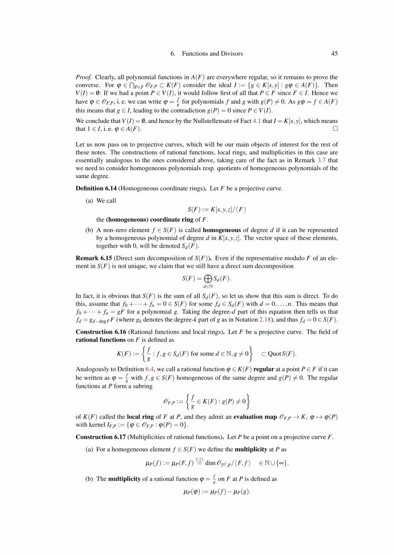
6. Functions and Divisors 45
Proof. Clearly, all polynomial functions in A(F) are everywhere regular, so it remains to prove theconverse. For ϕ ∈
⋂P∈F OF,P ⊂ K(F) consider the ideal I := {g ∈ K[x,y] : gϕ ∈ A(F)}. Then
V (I) = /0: If we had a point P ∈ V (I), it would follow first of all that P ∈ F since F ∈ I. Hence wehave ϕ ∈ OF,P, i. e. we can write ϕ = f
g for polynomials f and g with g(P) 6= 0. As gϕ = f ∈ A(F)
this means that g ∈ I, leading to the contradiction g(P) = 0 since P ∈V (I).
We conclude that V (I) = /0, and hence by the Nullstellensatz of Fact 4.1 that I =K[x,y], which meansthat 1 ∈ I, i. e. ϕ ∈ A(F). �
Let us now pass on to projective curves, which will be our main objects of interest for the rest ofthese notes. The constructions of rational functions, local rings, and multiplicities in this case areessentially analogous to the ones considered above, taking care of the fact as in Remark 3.7 thatwe need to consider homogeneous polynomials resp. quotients of homogeneous polynomials of thesame degree.
Definition 6.14 (Homogeneous coordinate rings). Let F be a projective curve.
(a) We callS(F) := K[x,y,z]/〈F 〉
the (homogeneous) coordinate ring of F .
(b) A non-zero element f ∈ S(F) is called homogeneous of degree d if it can be representedby a homogeneous polynomial of degree d in K[x,y,z]. The vector space of these elements,together with 0, will be denoted Sd(F).
Remark 6.15 (Direct sum decomposition of S(F)). Even if the representative modulo F of an ele-ment in S(F) is not unique, we claim that we still have a direct sum decomposition
S(F) =⊕d∈N
Sd(F).
In fact, it is obvious that S(F) is the sum of all Sd(F), so let us show that this sum is direct. To dothis, assume that f0 + · · ·+ fn = 0 ∈ S(F) for some fd ∈ Sd(F) with d = 0, . . . ,n. This means thatf0 + · · ·+ fn = gF for a polynomial g. Taking the degree-d part of this equation then tells us thatfd = gd−degF F (where gk denotes the degree-k part of g as in Notation 2.18), and thus fd = 0∈ S(F).
Construction 6.16 (Rational functions and local rings). Let F be a projective curve. The field ofrational functions on F is defined as
K(F) :={
fg
: f ,g ∈ Sd(F) for some d ∈ N,g 6= 0}⊂ QuotS(F).
Analogously to Definition 6.4, we call a rational function ϕ ∈K(F) regular at a point P∈ F if it canbe written as ϕ = f
g with f ,g ∈ S(F) homogeneous of the same degree and g(P) 6= 0. The regularfunctions at P form a subring
OF,P :={
fg∈ K(F) : g(P) 6= 0
}of K(F) called the local ring of F at P, and they admit an evaluation map OF,P→ K, ϕ 7→ ϕ(P)with kernel IF,P := {ϕ ∈ OF,P : ϕ(P) = 0}.
Construction 6.17 (Multiplicities of rational functions). Let P be a point on a projective curve F .
(a) For a homogeneous element f ∈ S(F) we define the multiplicity at P as
µP( f ) := µP(F, f ) 3.21= dimOP2,P/〈F, f 〉 ∈ N∪{∞}.
(b) The multiplicity of a rational function ϕ = fg on F at P is defined as
µP(ϕ) := µP( f )−µP(g).

46 Andreas Gathmann
It follows in the same way as in the affine case in Construction 6.6 that these multiplicities arewell-defined and additive. The notions of (orders of) zeros and poles are also carried over directly.
Remark 6.18 (Affine and projective local rings). As in Construction 3.20, for a point P = (x0 :y0 :1)on a projective curve F one can check that there is an isomorphism
OF,(x0 :y0 :1)→ OF i,(x0,y0),
fg7→ f i
gi
sending IF,(x0 :y0 :1) to IF i,(x0,y0). Hence the algebraic properties of the local ring as e. g. in Proposition
6.10, Remark 6.11, and Corollary 6.12 carry over directly from the affine to the projective case.
Exercise 6.19. Consider the rational function ϕ = x2
y2+yz on the projective curve F = y2z+ x3− xz2.Moreover, let P = (0:0 :1) ∈ F .
(a) Compute the order n = µP(ϕ).
(b) Determine a local coordinate t ∈ OF,P.
(c) Give an explicit description of ϕ in the form ϕ = ctn for a unit c ∈ OF,P, where c shouldbe written as f
g for some homogeneous f ,g ∈ S(F) of the same degree with f (P) 6= 0 andg(P) 6= 0.
Exercise 6.20.(a) Let P be a point on an affine curve F . Show that there is a rational function ϕ ∈ K(F) which
has exactly one pole which is of order 1 and at P, i. e. such that µP(ϕ) =−1 and µQ(ϕ)≥ 0for all Q 6= P.
(b) Let P1 and P2 be distinct points on a projective conic F . Show that there is a rational functionϕ ∈ K(F) with µP1(ϕ) = 1, µP2(ϕ) =−1, and µP(F) = 0 at all other points P of F .
Exercise 6.21. Let F be an affine curve. Prove that the affine field of rational functions K(F) isisomorphic to the projective one K(Fh).
Before we continue our study of multiplicities of rational functions on projective curves let us in-troduce the so-called divisors, a very convenient piece of notation that allows us to consider themultiplicities at all points of curve at once. We could have done this already in the affine case, buthave chosen not to do so as we will only consider projective curves from now on.
Definition 6.22 (Divisors). Let F be a projective curve.
(a) A divisor on F is a formal finite linear combination a1P1 + · · ·+ anPn of distinct pointsP1, . . . ,Pn ∈F with integer coefficients a1, . . . ,an ∈Z for some n∈N. Obviously, the divisorson F form an Abelian group under pointwise addition of the coefficients. We will denote itby DivF .
Equivalently, in algebraic terms DivF is just the free Abelian group generated by the pointsof F (i. e. the group of maps V (F)→ Z being non-zero at only finitely many points; with apoint mapping to its coefficient in the sense above).
(b) A divisor D = a1P1 + · · ·+anPn as above is called effective, written D ≥ 0, if ai ≥ 0 for alli = 1, . . . ,n. If D1,D2 are two divisors with D2−D1 effective, we also write this as D2 ≥D1or D1 ≤ D2. In other words, we have D2 ≥ D1 if and only if the coefficient of any point inD2 is greater than or equal to the coefficient of this point in D1.
(c) The degree of a divisor D = a1P1 + · · ·+ anPn is the number degD := a1 + · · ·+ an ∈ Z.Obviously, the degree is a group homomorphism deg: DivF → Z. Its kernel is denoted by
Div0 F = {D ∈ DivF : degD = 0}.
Note that the name “divisor” in this context is entirely unrelated to the idea of elements of ringsdividing one another. Instead, divisors are just given by multiplicities attached to all points on acurve, as appearing naturally in the following situations.

6. Functions and Divisors 47
Construction 6.23 (Divisors from polynomials and rational functions). Again, let F be a projectivecurve. The multiplicities of polynomials and rational functions of Construction 6.17 allow us todefine divisors on F as follows.
(a) For a non-zero homogeneous polynomial f ∈ S(F)\{0} the divisor of f is defined to be
div f := ∑P∈F
µP( f ) ·P ∈ DivF.
Hence, the effective divisor div f contains the data of the zeros of f together with theirmultiplicities. Note that the sum runs formally over all points of F — but as the number ofzeros of f is finite by Remark 3.19, there are only finitely many points in this sum with anon-zero multiplicity, so that we obtain a well-defined divisor.
(b) Similarly, for a non-zero rational function ϕ ∈ K(F)∗ we set
divϕ := ∑P∈F
µP(ϕ) ·P ∈ DivF.
This divisor is not effective; it encodes the zeros and poles of ϕ together with their mul-tiplicities. By definition, if we write ϕ = f
g as a quotient of two non-zero homogeneouspolynomials f ,g ∈ S(F)\{0} of the same degree then divϕ = div f −divg.
Example 6.24. Consider the rational function ϕ = yx on the projective curve F = y2 + yz+ x2 over
C, i. e. on the projective closure of the affine curve in Example 6.7. We have seen in this examplethat ϕ has a zero of order 1 at (0:0 :1). Apart from this point, it is easy to check that the only otherpoint at which y or x vanishes is (0: −1:1), where
µ(0:−1:1)(ϕ) = µ(0:−1:1)(y)−µ(0:−1:1)(x) = 0−1 =−1.
Hence the divisor of ϕ isdivϕ = 1 · (0:0 :1)−1 · (0: −1:1).
Exercise 6.25. Let F = y2z− x3 + xz2. Compute the divisor div yz on F .
Remark 6.26 (Additivity of multiplicities for divisors). Let F be a projective curve. The additivityof multiplicities as in Constructions 6.6 and 6.17 translates immediately into the following statementsfor divisors:
(a) For two homogeneous polynomials f ,g ∈ S(F)\{0} we get
div( f g) = ∑P∈F
µP( f g) ·P = ∑P∈F
µP( f ) ·P+ ∑P∈F
µP(g) ·P
= div f +divg.
(b) In the same way we obtain
div(ϕψ) = divϕ +divψ
for any two non-zero rational functions ϕ,ψ ∈ K(F)∗. In particular, this means that the mapdiv : K(F)∗→ DivF is a group homomorphism.
It is also very useful to translate the important theorems of Bézout and Noether of Chapter 4 into thelanguage of divisors.
Remark 6.27 (Bézout’s Theorem for divisors). For a projective curve F , Bézout’s Theorem ofCorollary 4.6 implies for the degrees of the divisors of Construction 6.23:
(a) for a non-zero homogeneous polynomial f ∈ S(F)\{0}
degdiv f = ∑P∈F
µP( f ) = ∑P∈F
µP(F, f ) = degF ·deg f ;
48 Andreas Gathmann
(b) for a non-zero rational function ϕ ∈ K(F)∗ (which we can write as ϕ = fg with f and g
non-zero and homogeneous of the same degree)
degdivϕ = degdiv f −degdivg(a)= degF ·deg f −degF ·degg = 0,
i. e. that “a rational function on a projective curve has equally many zeros as poles”. Inparticular, the image of the group homomorphism div : K(F)∗→ DivF of Remark 6.26 (b)lies in Div0 F .
Proposition 6.28 (Noether’s Theorem for divisors). Let F be a projective curve, and let g,h ∈ S(F)be non-zero homogeneous polynomials with divg≤ divh.
Then there is a homogeneous polynomial b ∈ S(F) (of degree degh− degg) with h = bg in S(F),and thus with divh = divb+divg.
Proof. As divg ≤ divh means µP(g) ≤ µP(h) for all P ∈ F , Noether’s Theorem as in Corollary4.12 (a) implies that there are homogeneous polynomials a and b (of degrees degh− degF anddegh− degg, respectively) such that h = aF + bg in K[x,y,z], and hence h = bg in S(F). Theequation divh = divb+divg now follows directly from Remark 6.26 (a) (or Corollary 4.12 (b)). �
As a first consequence of these statements we can identify the rational functions that are regular atevery point of the curve. Analogously to Proposition 6.13 we expect such functions to be polynomi-als — but in the projective case polynomials are only well-defined functions if they are constants:
Corollary 6.29 (Global regular functions on projective curves). Let F be a projective curve. Then⋂P∈F
OF,P = K ⊂ K(F),
i. e. the only rational functions that are everywhere regular on F are constants.
Proof. Let ϕ = fg ∈K(F) be regular at all points P∈F . This means that 0≤ µP(ϕ) = µP( f )−µP(g)
for all P, and hence that divg≤ div f . As f and g have the same degree, Proposition 6.28 then impliesthat f = cg for a constant c, and hence that ϕ = f
g = c is a constant. �
Remark 6.30 (Recovering rational functions from their divisors). Corollary 6.29 implies that arational function ϕ ∈ K(F)∗ on a projective curve F is determined up to scalars by its divisor divϕ:If ψ is another rational function with divψ = divϕ then div ψ
ϕ= 0 by Remark 6.26 (b), hence ψ
ϕis
some constant c ∈ K∗ by Corollary 6.29, and thus ψ = cϕ .
By definition, the group DivF of divisors on a projective curve F is a very large free Abelian group.As such, it is not very interesting from a group-theoretic point of view. It turns out that we can get amuch smaller and more interesting group by considering a certain quotient of DivF as follows.
Definition 6.31 (Divisor classes and Picard groups). Let F be a projective curve.
(a) A divisor on F is called principal if it is the divisor of a non-zero rational function as inConstruction 6.23 (b). The set of all principal divisors will be denoted by
PrinF := {divϕ : ϕ ∈ K(F)∗}.As the image of the group homomorphism div : K(F)∗ → DivF of Remark 6.26 (b) it isclearly a subgroup of DivF , and by Remark 6.27 (b) also of Div0 F .
(b) The quotient groupPicF := DivF/PrinF
is called the Picard group or group of divisor classes on F . Two divisors D1 and D2 definingthe same element in PicF , i. e. with D1−D2 = divϕ for a rational function ϕ ∈ K(F)∗, aresaid to be linearly equivalent, written D1 ∼ D2. Restricting to divisors of degree 0, we alsoset
Pic0 F := Div0 F/PrinF,which is a subgroup of PicF .

6. Functions and Divisors 49
10
Remark 6.32. By the homomorphism theorem, the degree of divisors induces isomorphismsDivF/Div0 F ∼= Z and PicF/Pic0 F ∼= Z. This means that the Picard group PicF and its degree-0part Pic0 F carry essentially the same information. It just depends on the specific application in mindwhether it is more convenient to work with PicF or Pic0 F .
Example 6.33 (Picard groups for curves of degree at most 2).(a) Let F be a projective line. For any point P ∈ F let lP be a line through P different from F ,
so that P is the only intersection point of F and lP (with multiplicity 1), and hence div lP = Pon F . For another point Q ∈ F we then obtain a rational function lP
lQwhose divisor is P−Q,
so that P−Q∼ 0 by definition of linear equivalence.
Now any divisor D of degree 0 can be written as D = P1 + · · ·+Pn−Q1−·· ·−Qn for somepoints P1, . . . ,Pn,Q1, . . . ,Qn on F , and hence we conclude that
D = (P1−Q1)+ · · ·+(Pn−Qn)∼ 0,
so that Pic0 F = {0} is the trivial group.
(b) If F is a projective conic we have seen in Exercise 6.20 (b) that for any two points P and Qon F there is again a rational function with divisor P−Q, so that P ∼ Q. So we concludeagain that Pic0 F = {0} in the same way as in (a).
For curves of bigger degree however, the Picard group is never trivial:
Proposition 6.34. Let F be a curve of degree d ≥ 3. Then P 6∼ Q for any two distinct points P andQ on F. In particular, Pic0 F is non-trivial.
Proof. Assume that P ∼ Q, i. e. that P−Q = div fg for some homogeneous polynomials f and g of
the same degree. Pick any line l through Q that does not pass through P and that is not the tangentTQF . Then div l = E +Q for an effective divisor E of degree degE = d−1≥ 2 that does not containP or Q. As
div( f l) = divg+divfg+div l = divg+P−Q+E +Q = divg+E +P≥ divg
it follows from Noether’s Theorem in Proposition 6.28 that there is a line l′ with div l′ = E +P.
But degE ≥ 2 means that E contains at least two points (or one point with multiplicity at least 2).By construction these points are not P or Q, and thus l and l′ have to pass through them (resp. betangent to F at the one point with multiplicity at least 2). As this fixes the line uniquely, it followsthat l = l′, and hence that P = Q.
We conclude that P 6∼ Q for P 6= Q, and thus that P−Q 6= 0 ∈ Pic0 F . �
Corollary 6.35 (Embedding of a curve in its Picard group). Let P0 be a fixed base point on a pro-jective curve F of degree at least 3. Then the map
Φ : V (F)→ Pic0 F, P 7→ P−P0
is injective.
Proof. If Φ(P) = Φ(Q) then P−P0 ∼ Q−P0, hence P ∼ Q, and thus P = Q as points in V (F) byProposition 6.34. �
Remark 6.36. For a projective curve F of degree degF ≥ 3, Corollary 6.35 gives us a naturalembedding (after choosing a base point) of the curve F into its degree-0 Picard group Pic0 F . Thisis a very interesting statement, as it gives us a natural map between mathematical objects of totallydifferent types (namely a variety and a group).
In the next chapter we will see that this map is even a bijection if degF = 3, making this correspon-dence between varieties and groups even more surprising and useful.

50 Andreas Gathmann
Exercise 6.37. Let F be a projective curve, and let f be a homogeneous polynomial with div f =D+E for two divisors D and E on F . Show: If D′ is linearly equivalent to D and D′+E is effectivethen there is a homogeneous polynomial g with divg = D′+E.
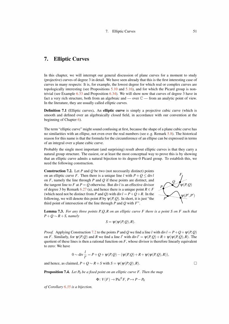
7. Elliptic Curves 51
7. Elliptic Curves
In this chapter, we will interrupt our general discussion of plane curves for a moment to study(projective) curves of degree 3 in detail. We have seen already that this is the first interesting case ofcurves in many respects: It is, for example, the lowest degree for which real or complex curves aretopologically interesting (see Propositions 5.10 and 5.16), and for which the Picard group is non-trivial (see Example 6.33 and Proposition 6.34). We will show now that curves of degree 3 have infact a very rich structure, both from an algebraic and — over C — from an analytic point of view.In the literature, they are usually called elliptic curves.
Definition 7.1 (Elliptic curves). An elliptic curve is simply a projective cubic curve (which issmooth and defined over an algebraically closed field, in accordance with our convention at thebeginning of Chapter 6).
The term “elliptic curve” might sound confusing at first, because the shape of a plane cubic curve hasno similarities with an ellipse, not even over the real numbers (see e. g. Remark 5.8). The historicalreason for this name is that the formula for the circumference of an ellipse can be expressed in termsof an integral over a plane cubic curve.
Probably the single most important (and surprising) result about elliptic curves is that they carry anatural group structure. The easiest, or at least the most conceptual way to prove this is by showingthat an elliptic curve admits a natural bijection to its degree-0 Picard group. To establish this, weneed the following construction.
Construction 7.2. Let P and Q be two (not necessarily distinct) pointson an elliptic curve F . Then there is a unique line l with P+Q ≤ div lon F , namely the line through P and Q if these points are distinct, andthe tangent line to F at P = Q otherwise. But div l is an effective divisorof degree 3 by Remark 6.27 (a), and hence there is a unique point R ∈ F(which need not be distinct from P and Q) with div l = P+Q+R. In thefollowing, we will denote this point R by ψ(P,Q). In short, it is just “thethird point of intersection of the line through P and Q with F”.
F
ψ(P,Q)
P′ψ(P′,P′)
QP
Lemma 7.3. For any three points P,Q,R on an elliptic curve F there is a point S on F such thatP+Q∼ R+S, namely
S = ψ(ψ(P,Q),R).
Proof. Applying Construction 7.2 to the points P and Q we find a line l with div l = P+Q+ψ(P,Q)on F . Similarly, for ψ(P,Q) and R we find a line l′ with div l′ = ψ(P,Q)+R+ψ(ψ(P,Q),R). Thequotient of these lines is then a rational function on F , whose divisor is therefore linearly equivalentto zero: We have
0∼ divll′= P+Q+ψ(P,Q)− (ψ(P,Q)+R+ψ(ψ(P,Q),R)),
and hence, as claimed, P+Q∼ R+S with S = ψ(ψ(P,Q),R). �
Proposition 7.4. Let P0 be a fixed point on an elliptic curve F. Then the map
Φ : V (F)→ Pic0 F, P 7→ P−P0
of Corollary 6.35 is a bijection.
52 Andreas Gathmann
Proof. As we already know by Corollary 6.35 that Φ is injective, it remains to prove surjectivity. Solet D be an arbitrary element of Pic0 F , which we can write as
D = P1 + · · ·+Pm−Q1−·· ·−Qm
for some m ∈ N>0 and not necessarily distinct points P1, . . . ,Pm,Q1, . . . ,Qm ∈ F . Assume first thatm≥ 2. By Lemma 7.3 there is then a point S ∈ F with P1 +P2 ∼ Q1 +S, and hence
D∼ S+P3 + · · ·+Pm−Q2−·· ·−Qm.
Up to linear equivalence, we have thus reduced the number m of (positive and negative) points in Dby 1. Continuing this process as long as m ≥ 2, we see that D ∼ P−Q for some P,Q ∈ F . In thesame way, Lemma 7.3 now gives us a point T with P+P0 ∼ Q+T , i. e. with D∼ P−Q∼ T −P0.But this means that Φ(T ) = D, i. e. that Φ is surjective. �
Remark 7.5. Let F be an elliptic curve. After choosing a base point P0 ∈ F , Proposition 7.4 givesus a canonical bijection between the variety V (F) and the Abelian group Pic0 F , i. e. between twovery different types of mathematical objects. We can use it to give V (F) the structure of an Abeliangroup, and Pic0 F the structure of a smooth projective variety.
In fact, it can be shown that Pic0 F can be made into a variety (the so-called Picard variety) for everysmooth projective curve F . In contrast, the statement that V (F) has a natural structure of an Abeliangroup is very special to elliptic curves. Let us explore this group structure in more detail.
Construction 7.6 (The group structure on an elliptic curve). Let P0 be a fixed base point on anelliptic curve F . As in Remark 7.5, we can use Proposition 7.4 to define a group structure on V (F)in such a way that the map Φ becomes an isomorphism of groups. More precisely, if we denote thisgroup operation on V (F) by the symbol ⊕ (to distinguish it from the addition of points in DivF orPicF), then P⊕Q for P,Q ∈ F is the unique point of F satisfying
Φ(P⊕Q) = Φ(P)+Φ(Q),
where “+” denotes the addition of divisors in Pic0 F . We can use Lemma 7.3 to solve this for P⊕Q:
P⊕Q = Φ−1(Φ(P)+Φ(Q))
= Φ−1(P−P0 +Q−P0)
= Φ−1(P+Q−2P0)
7.3= Φ
−1(P0 +ψ(ψ(P,Q),P0)−2P0)
= Φ−1(ψ(ψ(P,Q),P0)−P0)
= ψ(ψ(P,Q),P0).
In other words, to construct the point P⊕Q we draw a line through P and Q. Then we draw anotherline through the third intersection point ψ(P,Q) of this line with F and the point P0. The thirdintersection point of this second line with F is then P⊕Q, as in the picture below on the left.
Similarly, for the inverse P of P in the above group structure we obtain
P = Φ−1(−Φ(P))
= Φ−1(P0−P)
= Φ−1(P0 +P0−P−P0)
7.3= Φ
−1(P+ψ(ψ(P0,P0),P)−P−P0)
= ψ(ψ(P0,P0),P).
So to construct the inverse P we draw the tangent to F through P0. Then we draw another linethrough the other intersection point ψ(P0,P0) of this tangent with F and the point P. The thirdintersection point of this second line with F is P, as in the following picture.

7. Elliptic Curves 53
F F
Q P
P0
P⊕Q
P P
P0
Note that, using this geometric description, the operation ⊕ could also be defined in a completelyelementary way, without referring to the theory of divisors. However, it would then be very difficultto show that we obtain a group structure in this way, in particular to prove associativity.
Remark 7.7 (Non-algebraically closed fields). Let K′ be a subfield of K which is not necessarilyalgebraically closed, and assume that F ∈ K′[x,y,z] is defined over K′. Note that for two pointsP,Q ∈V (F)∩P2
K′ on F with coordinates in K′ the point ψ(P,Q) then lies in V (F)∩P2K′ as well: The
polynomial F restricted to the line through P and Q is a cubic homogeneous polynomial over K′ thatsplits off two linear factors over K′ corresponding to its zeros P and Q. Hence the remaining linearfactor corresponding to ψ(P,Q) is also defined over K′, which means that ψ(P,Q) ∈V (F)∩P2
K′ .
Choosing the base point P0 in V (F)∩P2K′ , we can therefore restrict the group structure on V (F) to
V (F)∩P2K′ , obtaining a subgroup of V (F).
Example 7.8 (Elliptic Curve Cryptography). There is an interesting application of the group struc-ture on an elliptic curve to cryptography. The key observation is that “multiplication is easy, butdivision is hard”. More precisely, assume that we are given a specific elliptic curve F and a basepoint P0 ∈ F for the group structure. In view of Remark 7.7, the ground field for the curve does nothave to be algebraically closed; in fact, for practical computations one has to choose a finite field inorder to avoid rounding errors in the computations.
(a) Given P ∈ V (F) and n ∈ N, the n-fold addition n�P := P⊕·· ·⊕P can be computed veryquickly, even for very large n (think of numbers with hundreds of digits):• By repeatedly applying the operation P 7→ P⊕P, we can compute all points 2k�P for
all k such that 2k ≤ n.• Now we just have to add these points 2k�P for all k such that the k-th digit in the
binary representation of n is 1.This computes the point n�P in a time proportional to logn (i. e. in a very short time).
(b) On the other hand, given two sufficiently general points P,Q∈V (F) it is essentially impossi-ble to compute an integer n∈N such that n�P = Q (in case such a number exists). Note thatthis is not a mathematically precise statement — there is just no known algorithm that canperform the “inverse” of the multiplication of (a) in shorter time than a simple trial-and-errorapproach (which would be impractical for large n).
Let us now assume that Alice and Bob want to establish an encrypted communication over an inse-cure channel, but that they have not met in person before, so that they could not secretly agree ona key for the encryption. Using the above idea, they can then agree (publicly) on a ground field K,a specific elliptic curve F over K, a base point P0 ∈ V (F), and another point P ∈ V (F). Now Alicepicks a secret (very large) integer n, computes n�P as in (a), and sends (the coordinates of) thispoint to Bob. In the same way, Bob chooses a secret number m, computes m�P, and sends thispoint to Alice.As Alice knows her secret number n and the point m�P from Bob, she can then compute the pointmn�P = n� (m�P). In the same way, Bob can compute this point as mn�P = m� (n�P) aswell. But except for the data of the chosen curve the only information they have exchanged publiclywas P, n�P, and m�P, and by (b) it is not possible in practice to recover n or m, and hence mn�P,from these data. Hence Alice and Bob can use (the coordinates of) mn�P as a secret key for theirencrypted communication.
54 Andreas Gathmann
Exercise 7.9. Let F be an elliptic curve of the form
F = y2z− x3−λxz2−µz3
for some given λ ,µ ∈ K (it can be shown that every elliptic curve can be brought into this form bya change of coordinates if the characteristic of K is not 2 or 3). Pick the point P0 = (0:1 :0) ∈ F asthe base point for the group structure on F .
For given points P and Q on F compute explicitly the coordinates of the sum P⊕Q and the inverseP in terms of the coordinates of P and Q.
11Let us now restrict our attention to the ground field C, so that an elliptic curve is topologically atorus by Example 5.17 (a). In the remaining part of this chapter we want to see how these tori andelliptic curves arise in complex analysis in a totally different way. As we have not developed anyanalytic techniques in these notes we will only sketch most arguments; more details can be founde. g. in [Ki, Section 5.1]. Let us start by giving a quick review of what we will need from standardcomplex analysis. As usual, we will denote a complex variable in C by z. In contrast, for the restof this chapter the homogeneous coordinates of P2
C will be called x0,x1,x2 instead of x,y,z to avoidconfusion.
Remark 7.10 (Holomorphic and meromorphic functions). Let U ⊂C be an open subset. Recall thata function f : U →C is called holomorphic if it is complex differentiable at all points z0 ∈U , i. e. ifthe limit
f ′(z0) := limz→z0
f (z)− f (z0)
z− z0exists. A function f : U → C∪{∞} is called meromorphic if it is holomorphic except for some iso-lated singularities which are all poles, i. e. if for all z0 ∈U there is a number n∈Z and a holomorphicfunction f̃ in a neighborhood of z0 in U in which
f (z) = (z− z0)n · f̃ (z).
If f does not vanish identically in a neighborhood of z0 we can moreover assume that f̃ (z0) 6= 0 inthis representation; the number n is then uniquely determined. We will call it the multiplicity of fat z0 and denote it by µz0( f ). It is obviously the analogue of the multiplicity of a rational functionas in Construction 6.6 and Proposition 6.10 (b). The notions of (orders of) zeros and poles areused for meromorphic functions in the same way as for rational functions. Note that every rationalfunction (i. e. every quotient of polynomials) in z is clearly meromorphic; there are however manymore meromorphic than rational functions as e. g. the exponential function z 7→ ez.
Remark 7.11 (Properties of holomorphic and meromorphic functions). Although the definition ofholomorphic, i. e. complex differentiable functions is formally exactly the same as that of real differ-entiable functions, the behavior of the complex and real cases is totally different. The most notabledifferences that we will need are:
(a) Every holomorphic function f is analytic, i. e. it can be represented locally around everypoint z0 by its Taylor series. Consequently, a meromorphic function f of order n at z0 canlocally be expanded in a Laurent series as f (z) = ∑
∞k=n ck (z− z0)
k, with n = µz0( f ) [G4,Proposition 9.8]. The coefficient c−1 of this series is called the residue of f at z0 and denotedby resz0 f .
(b) (Residue Theorem) If γ is a closed (positively oriented) path in C and f is a meromorphicfunction in a neighborhood of γ and its interior, without poles on γ itself, then∫
γ
f (z)dz = 2πi ∑z0
resz0 f ,
with the sum taken over all z0 in the interior of γ (at which f has poles) [G4, Proposition11.13]. In particular, if f is holomorphic in the interior of γ then this integral vanishes.
(c) (Liouville’s Theorem) Every function that is holomorphic and bounded on the whole com-plex plane C is constant [G4, Proposition 8.2].

7. Elliptic Curves 55
Construction 7.12 (Tori from lattices). As mentioned above, forour applications to elliptic curves we have to construct a torus.To do this, fix two complex numbers ω1,ω2 ∈ C that are linearlyindependent over R, i. e. that do not lie on the same real line in Cthrough the origin. Then
Λ = Zω1 +Zω2 = {mω1 +nω2 : m,n ∈ Z} ⊂ Cis called a lattice in C, as indicated by the points in the picture onthe right. It is an additive subgroup of C, and the quotient C/Λ istopologically a torus.
Reω1
ω2
Im
For the rest of this chapter, Λ will always be a fixed lattice in C. Note that functions on the torus C/Λ
correspond exactly to Λ-periodic functions on C, i. e. to functions f on C with f (z+ω) = f (z) forall z ∈C and ω ∈ Λ. In the following, we will use the concepts of functions on C/Λ and Λ-periodicfunctions on C interchangeably.
It is our goal to show that the torus C/Λ can be identified with an elliptic curve in a natural way. Letus start with a first auxiliary result that already indicates the similarities between the algebraic andanalytic setting: We will show the analytic analogue of Remark 6.27 (b), namely that a meromorphicfunction on the torus C/Λ has equally many zeros as poles.
Lemma 7.13. Let f : C/Λ→ C∪{∞} be a non-zero meromorphic function. Then
∑z0∈C/Λ
µz0( f ) = 0.
Proof sketch. Let γ be the path around a “parallelogram of period-icity” as in the picture on the right, i. e. a parallelogram with sidevectors spanning Λ. We choose it so that the zeros and poles of fdo not lie on γ , and hence have a unique representative inside thisparallelogram. It follows that∫
γ
f ′(z)f (z)
dz = 0 (∗)
since the integrals along opposite sides of the parallelogram canceleach other due to the periodicity of f .
Re
Im
γ
On the other hand, we can compute this integral using the Residue Theorem of Remark 7.11 (b):At a point z0 with µz0( f ) = n so that we can write f (z) = (z− z0)
n f̃ (z) with f̃ holomorphic andnon-zero around z0 as in Remark 7.10 we have
resz0
f ′
f= resz0
n(z− z0)n−1 f̃ +(z− z0)
n f̃ ′
(z− z0)n f̃= resz0
(n
z− z0+
f̃ ′
f̃
)= n = µz0( f ),
and hence we obtain by the Residue Theorem∫γ
f ′(z)f (z)
dz = 2πi ∑z0∈C/Λ
resz0
f ′
f= 2πi ∑
z0∈C/Λ
µz0( f ).
Comparing this with (∗) then gives the desired result. �
Remark 7.14 (Residue Theorem on manifolds). In the same way as Remark 6.27 (b), Lemma 7.13does not only hold for a torus C/Λ, but also for an arbitrary compact 1-dimensional complex mani-fold X , and thus for any (smooth) complex projective curve. Let us briefly explain how to adapt theproof of Lemma 7.13 to this more general case.
The main step in this generalization is to extend the concepts of path integrals and the Residue Theo-rem from the complex plane to manifolds. This is not entirely straightforward, since the differentialdz in the integral depends on the choice of a local coordinate z on X . As a consequence, there is no

56 Andreas Gathmann
well-defined integral over a function on X since we would have to combine it with the coordinate-dependent dz to integrate it. Instead, we have to combine a function with a differential to obtainexpressions of the form ω = f dg for (meromorphic) functions f and g that satisfy the usual rules ofdifferentiation. Such objects are called differential forms on X .
In these notes we will use differential forms only in a few side remarks that will not be needed lateron, and hence we will not introduce them rigorously. Let us just mention that integrals and theResidue Theorem then behave as expected: For a closed path γ and a differential form ω on X nothaving any poles on γ itself, we can define an integral
∫γ
ω whose value can be computed by theResidue Theorem ∫
γ
ω = 2πi ∑P
resP ω
as in Remark 7.11 (b), where the sum is taken over all points P in the interior of γ , and the residueof ω at a point P is defined similarly to Remark 7.11 (a).
An additional benefit of this version of the Residue Theorem on manifolds is that we can exchangethe roles of the interior and exterior of γ: Consider a differential form ω on X with poles at somepoints (marked P1 and P2 in the picture below on the right). If we form the integral
∫γ
ω over a smallloop γ that contains none of these points, the result will be 0 by the Residue Theorem. But we canalso swap the roles of the interior and exterior of γ (without changing the value of the integral), sothat now all poles lie in the interior of γ , and the Residue Theorem gives us the sum over all residuesof ω . Comparing these two results we see that
∑P∈X
resP ω = 0,
which is also sometimes called the Residue Theorem (for man-ifolds) in the literature.
Applying this now to the differential form
ω = d(log f ) =f ′(z)f (z)
dz gives us ∑P∈X
resPf ′(z)f (z)
dz = 0, γ
P2
P1
X
and thus with the same (local) computation resPf ′(z)f (z) dz = µP( f ) as in the proof of Lemma 7.13
∑P∈X
µP( f ) = 0,
i. e. that f has equally many zeros as poles.
But let us now return to our study of the torus C/Λ. The key ingredient to identify it with the pointsof an elliptic curve is the following meromorphic function.
Proposition and Definition 7.15 (The Weierstraß ℘-function). There is a meromorphic function ℘
on C, called the Weierstraß ℘-function (pronounced like the letter “p”), defined by
℘(z) =1z2 + ∑
ω∈Λ\{0}
(1
(z−ω)2 −1
ω2
).
It has poles of order 2 exactly at the lattice points.
Proof sketch. It is a standard fact that an (infinite) sum of holomorphic functions is holomorphic atz0 provided that the sum converges uniformly in a neighborhood of z0. We will only sketch the proofof this convergence: Let z0 ∈ C\Λ be a fixed point that is not in the lattice. Then every summand isa holomorphic function in a neighborhood of z0. The expansions of these summands for large ω are
1(z−ω)2 −
1ω2 =
1ω2
(1
(1− zω)2 −1
)=
2zω3 +
(terms of order at least
1ω4
),
so the summands grow like ω3. Let us add up these values according to the absolute value of ω .Note that the number of lattice points with a given absolute value approximately equal to n ∈ N is

7. Elliptic Curves 57
roughly proportional to the area of the annulus with inner radius n− 12 and outer radius n+ 1
2 , whichgrows linearly with n. Hence the final sum is of the order ∑
∞n=1 n · 1
n3 = ∑∞n=1
1n2 , which is convergent.
Note that the sum would not have been convergent without the subtraction of the constant 1ω2 in each
summand, as then the individual terms would grow like 1ω2 , and therefore the final sum would be of
the type ∑∞n=1
1n , which is divergent.
Finally, the poles of order 2 at the points of Λ are clearly visible. �
Remark 7.16 (Properties of the ℘-function). One can show that in an absolutely convergent seriesas above all manipulations (reordering of the summands, term-wise differentiation) can be performedas expected. In particular, the following properties of the ℘-function are obvious:
(a) The ℘-function is an even function, i. e. ℘(z) =℘(−z) for all z ∈ C. Hence its Laurentseries at 0 as in Remark 7.11 (a) contains only even exponents.
(b) Its derivative is ℘′(z) = ∑ω∈Λ−2
(z−ω)3 . It is an odd function, i. e. ℘′(z) =−℘′(−z) for all z.In other words, its Laurent series at 0 contains only odd exponents. It has poles of order 3exactly at the lattice points.
(c) The℘-function is Λ-periodic, and hence gives a meromorphic function℘ : C/Λ→C∪{∞}.To show this note first that ℘′ is Λ-periodic by (b). Now, for given z0 ∈ C and ω ∈ Λ weintegrate ℘′ along the path γ = γ1 + γ2 + γ3 + γ4 shown in the picture below on the right.
Of course, the result is 0, since ℘ is an integral of ℘′.But also the integral along γ2 cancels the integral alongγ4 as ℘′(z) is periodic. The integral along γ3 is equal to℘(−ω
2 )−℘(ω
2 ), so it vanishes as well since℘ is an evenfunction. So we conclude that
0 =∫
γ1
℘′(z)dz =℘(z0 +ω)−℘(z0),
i. e. that ℘ is Λ-periodic.
Re
Im
ω
z0 z0 +ω
−ω
2ω
2
γ1
γ3
γ4 γ2
Lemma 7.17 (Differential equation of the℘-function). The℘-function satisfies a differential equa-tion
℘′(z)2 = c3℘(z)3 + c2℘(z)2 + c1℘(z)+ c0 for all z ∈ C
for some constants c0,c1,c2,c3 ∈ C (depending on Λ).
Proof. By Remark 7.16 (b) we know that (℘′)2 is an even function with a pole of order 6 at theorigin. Hence its Laurent series around 0 is of the form
℘′(z)2 =
a−6
z6 +a−4
z4 +a−2
z2 +a0 +(terms of positive multiplicity at 0)
for some constants a−6,a−4,a−2,a0 ∈ C. The functions ℘3, ℘2, ℘, and 1 are also even and havepoles at the origin of order 6, 4, 2, and 0, respectively. Hence there are constants c3,c2,c1,c0 ∈ Csuch that the Laurent series of the linear combination
f (z) :=℘′(z)2− c3℘(z)3− c2℘(z)2− c1℘(z)− c0
has only positive powers of z. This means that f is holomorphic around the origin and vanishes at 0.
But ℘ and ℘′, and hence also f , are Λ-periodic by Remark 7.16 (c). Hence f is holomorphicaround all lattice points. Moreover, f is holomorphic around all other points as well, as ℘ and ℘′
are. Hence f is holomorphic on all of C.
The Λ-periodicity means that every value taken on by f is already assumed on the parallelogram{xω1 + yω2 : x,y ∈ [0,1]}. As f is continuous, its image on this compact parallelogram, and henceon all of C, is bounded. So we see by Liouville’s Theorem of Remark 7.11 (c) that f must beconstant. But as we have already shown that f (0) = 0, it follows that f is the zero function, whichis exactly the statement of the lemma. �

58 Andreas Gathmann
Remark 7.18. By an explicit computation one can show that the coefficients c3,c2,c1,c0 in Lemma7.17 are given by
c3 = 4, c2 = 0, c1 =−60 ∑ω∈Λ\{0}
1ω4 , and c0 =−140 ∑
ω∈Λ\{0}
1ω6 .
The proof of Lemma 7.17 shows impressively the powerful methods of complex analysis: To proveour differential equation, i. e. the equality of the two functions (℘′)2 and c3℘
3 + c2℘2 + c1℘+ c0,
it was sufficient to just compare four coefficients of their Laurent expansions at the origin — the restthen follows entirely from general theory.
Note also that the differential equation of Lemma 7.17 is a (non-homogeneous) cubic equation inthe two functions ℘ and ℘′, which are Λ-periodic and thus well-defined on the quotient C/Λ. Wecan therefore use it to obtain a map from C/Λ to an elliptic curve as follows.
Proposition 7.19 (Complex tori as elliptic curves). Consider the elliptic curve
F = x22x0− c3x3
1− c2x21x0− c1x1x2
0− c0x30
for the constants c3,c2,c1,c0 ∈ C of Lemma 7.17. There is a bijection
Ψ : C/Λ→V (F), z 7→ (1:℘(z) :℘′(z)).
Proof. As ℘ and ℘′ are Λ-periodic and satisfy the differential equation of Lemma 7.17, it is clearthat Ψ is well-defined as a map to V (F). Strictly speaking, for z = 0 we have to note that ℘ and℘′ have poles of order 2 and 3, respectively, so that the given expression for Ψ(0) is of the form(1:∞ :∞). But by Remark 7.10 we can write ℘(z) = f (z)
z2 and ℘′(z) = g(z)z3 locally around the origin
for some holomorphic functions f ,g that do not vanish at 0, and so we have to interpret the expressionfor Ψ as
Ψ(0) = limz→0
(1:℘(z) :℘′(z)) = limz→0
(z3 :z f (z) :g(z)) = (0:0 :1),
i. e. Ψ(z) is well-defined at z = 0 as well.
Now let (x0 :x1 :x2) ∈V (F) be a given point; we have to show that it has exactly one inverse imageunder Ψ. By what we have just said this is obvious for the “point at infinity” (0:0 :1), so let usassume that we are not at this point and hence pass to inhomogeneous coordinates where x0 = 1. Wethus have to show that there is exactly one (non-zero) z ∈ C/Λ with ℘(z) = x1 and ℘′(z) = x2.
Recall that ℘, and thus also ℘− x1, has exactly one pole in C/Λ, namely the origin, and that thispole is of order 2. Hence ℘− x1 also has exactly two zeros (counted with multiplicities) in C/Λ byLemma 7.13, i. e. there are two z ∈C/Λ with ℘(z) = x1. For such a point z we then have by Lemma7.17
℘′(z)2 = c3℘(z)3 + c2℘(z)2 + c1℘(z)+ c0 = c3 x3
1 + c2 x21 + c1 x1 + c0 = x2
2
since (1:x1 :x2) ∈V (F). So there are two possibilities:
• ℘′(z) = 0: Then x2 = 0 as well, and z is a double zero (i. e. the only zero) of the function℘− x1. So there is exactly one z ∈ C/Λ with Ψ(z) = (1:℘(z) :℘′(z)) = (1:x1 :x2).
• ℘′(z) 6= 0: Then z is only a simple zero of ℘− x1. As ℘ is even and ℘′ odd by Remark7.16, we see that−z must be the other zero, and it satisfies℘′(−z) =−℘′(z). Hence exactlyone of the equations ℘′(z) = x2 and ℘′(−z) = x2 holds, and the corresponding point is theunique inverse image of (1:x1 :x2) under Ψ.
Altogether we conclude that Ψ is bijective, as we have claimed. �
Remark 7.20. In fact, the map Ψ of Proposition 7.19 is not just a bijection: Both C/Λ and V (F)are 1-dimensional complex manifolds in a natural way, and Ψ is even an isomorphism between thesetwo manifolds.

7. Elliptic Curves 59
Remark 7.21 (Group structures on elliptic curves). With Proposition 7.19 we are again in a similarsituation as in Proposition 7.4: We have a bijection between a group C/Λ and a variety V (F), so thatthe map Ψ of the above proposition can be used to construct a group structure on V (F). In fact, wewill see in Exercise 7.23 that this group structure is precisely the same as that obtained by the mapΦ of Proposition 7.4 using divisors. But the algebraic properties of this group structure is a lot moreobvious in this new picture: For example, the points of order n are easily read off to be the n2 points
1n(iω1 + jω2) for 0≤ i, j < n.
Exercise 7.22. Let Λ be a lattice in C. Show that there is no meromorphic function on C/Λ withexactly one pole, such that this pole is of order 1.
Note that by Lemma 7.13 such a function would then also have exactly one zero of order 1 on C/Λ
— so using the identification of C/Λ with an elliptic curve as in Proposition 7.19, we can interpretthe non-existence of such a function as an analytic analogue of the statement of Proposition 6.34.
Exercise 7.23. Let F be an elliptic curve corresponding to a torus C/Λ as in Proposition 7.19. Showthat the group structure on V (F) induced by Pic0 F as in Proposition 7.4 (using (0:0 :1) as the basepoint) is the same as the one induced by the natural group structure of C/Λ.
Exercise 7.24. Let Λ⊂ C be a lattice. Given two points z,w ∈ C/Λ, it is very easy to find a naturalnumber n such that n ·w = z (in the group structure of C/Λ), in case such a number exists. Why isthis no contradiction to the idea of the cryptographic application in Example 7.8?
12
60 Andreas Gathmann
8. The Riemann-Roch Theorem
In the previous two chapters we have introduced and studied rational and regular functions on pro-jective curves. As our last goal in these notes we now want to address the question how many suchfunctions there are on a given projective curve (which, as before, will always be assumed to besmooth over an algebraically closed field).But before we can try to solve this problem we first have to figure out what the precise questionshould be, i. e. which functions we want to consider and what exactly we mean by “how many”.Note that we know already by Corollary 6.29 that global regular functions on a projective curveare always constant, and thus not very interesting. On the other hand, to obtain arbitrary rationalfunctions we can take any quotient of two homogeneous polynomials of the same degree, so thatwe clearly get an infinite-dimensional vector space of such functions. Hence the most interestingquestion is to study something between regular and rational functions: rational functions which areeverywhere regular, except for some specific points at which we allow poles of a given maximalorder (or require zeros of a certain order). We will see that such functions form finite-dimensionalvector spaces, so that we can then ask for their dimensions.The conditions of allowing poles or requiring zeros at specified points is described best using thelanguage of divisors. This leads to the following spaces that we will consider in this chapter.
Construction 8.1 (L(D) and l(D)). Let D be a divisor on a projective curve F . We set
L(D) := {ϕ ∈ K(F)∗ : divϕ +D≥ 0}∪{0}.If D = ∑P∈F aP ·P, i. e. aP denotes the coefficient of P in D, the condition divϕ +D ≥ 0 obviouslymeans µP(ϕ)+aP ≥ 0, i. e. µP(ϕ)≥−aP, for all points P ∈ F . Hence, except for the zero function,L(D) consists by construction of all rational functions ϕ ∈ K(F)∗ that are just regular at all points ofF , except that
(a) ϕ may have a pole of order at most aP at P for all P with aP > 0, and(b) ϕ must have a zero of order at least −aP at P for all P with aP < 0.
Note that L(D) is a vector space over K: For all λ ∈ K and ϕ,ψ ∈ L(D), i. e. such that µP(ϕ)≥−aPand µP(ψ)≥−aP for all P ∈ F , we have
µP(ϕ +ψ)≥−aP by Corollary 6.12 and µP(λϕ) = µP(ϕ)≥−aP by Construction 6.6 (b)
for all P, and thus ϕ +ψ ∈ L(D) and λϕ ∈ L(D). Hence we can define
l(D) := dimL(D) ∈ N∪{∞}.
As motivated above, it is the goal of this chapter to compute these dimensions l(D). Unfortunately,we will not be able to do this for all D, since in general l(D) depends on the precise position ofthe points occurring in D in a complicated way. However, the Riemann-Roch Theorem in Corollary8.17 will allow to compute l(D) in many cases just from the degree of D, which is of course easyto read off. The formula will also involve the genus of the curve — a concept that we have alreadyseen over C from a topological point of view in Remark 5.12. As a byproduct of our work, we willtherefore also give an algebraic definition of the genus of a curve, which is then applicable to anyalgebraically closed ground field.But let us start with a few simple examples in which l(D) is easy to determine.
Example 8.2.(a) For the divisor D = 0 the space L(D) = L(0) is by definition just the set of all rational
functions that are regular at every point of the curve. Hence by Corollary 6.29 we haveL(0) = K, and thus l(0) = 1.

8. The Riemann-Roch Theorem 61
(b) For any divisor D with degD < 0 we have L(D) = {0} and thus l(D) = 0: If there was anon-zero element ϕ ∈ L(D) we would have divϕ +D≥ 0, and hence degdivϕ +degD≥ 0by taking degrees. But this is a contradiction to degD < 0 since degdivϕ = 0 by Remark6.27 (b).
Remark 8.3. Let D be a divisor on a projective curve F .
(a) If D′ is another divisor on F with D≤ D′ then L(D)⊂ L(D′) and hence l(D)≤ l(D′), sincedivϕ +D≥ 0 clearly implies divϕ +D′ ≥ divϕ +D≥ 0.
(b) If D′ ∼ D is linearly equivalent, i. e. D−D′ = divψ for a rational function ψ ∈ K(F)∗, thenL(D)→ L(D′), ϕ 7→ψϕ is an isomorphism of vector spaces (with inverse ϕ 7→ ϕ
ψ) since the
condition divϕ +D≥ 0 is equivalent to div(ψϕ)+D′ ≥ 0. Hence we have l(D) = l(D′) inthis case.
In particular, the notion l( ·) is also well-defined for elements of the Picard group PicF . Inthe following, we will also use it in this extended way.
Many of our strategies to compute the numbers l(D) will be inductive, i. e. relate l(D) to l(D±P)for a point P on the curve. Of particular importance will therefore be the following result, whichtells us that l(D) changes at most by 1 when adding or subtracting a point from D.
Lemma 8.4. Let D be a divisor on a projective curve F.
(a) For any point P ∈ F we have l(D+P) = l(D) or l(D+P) = l(D)+1.
(b) For any divisor D′ ≥ D we have l(D)≤ l(D′)≤ l(D)+deg(D′−D).
Proof.
(a) As D≤ D+P we have L(D)⊂ L(D+P), and hence l(D)≤ l(D+P), by Remark 8.3 (a).
Now let aP be the coefficient of P in D, so that aP + 1 is the coefficient of P in D+ P.Consider the linear map
Φ : L(D+P)→ K, ϕ 7→ (taP+1ϕ)(P),
where t is a local coordinate around P as in Proposition 6.10. Note that this evaluation oftaP+1ϕ at P is well-defined, since for ϕ ∈ L(D+P)\{0} we have
µP(taP+1ϕ) = µP(ϕ)+aP +1≥ 0 (∗)
(where the last inequality follows from Construction 8.1), so that taP+1ϕ is regular at P byProposition 6.10 (b).
The kernel of Φ consists exactly of the rational functions for which taP+1ϕ has a zero at P,i. e. for which we have strict inequality in (∗). As this is equivalent to µP(ϕ)+ aP ≥ 0 andthus to divϕ +D ≥ 0, we conclude that kerΦ = L(D). The homomorphism theorem thusyields
L(D+P)/L(D)∼= imΦ ⊂ K,
which means that l(D+P) = l(D) (in case imΦ = {0}) or l(D+P) = l(D)+ 1 (in caseimΦ = K).
(b) This follows immediately from (a) by induction on deg(D′−D), since D′ is obtained fromD by adding deg(D′−D) points. �
Remark 8.5. The proof of Lemma 8.4 (a) also has a simple analytic interpretation in case of theground field K =C. As the multiplicity of a rational function ϕ ∈ L(D+P) at P is at least−aP−1, itsLaurent expansion as in Remark 7.11 (a) can be taken to start with the power t−aP−1 of an (analytic)local coordinate t. Inside L(D+P), the subspace L(D) now consists of exactly those functions forwhich the t−aP−1-coefficient of this expansion vanishes. As this coefficient is one complex number,its vanishing imposes one condition on L(D+P) — which can be trivially satisfied by all elementsof L(D+P) already (in which case l(D) = l(D+P)) or not (in which case l(D) = l(D+P)−1).

62 Andreas Gathmann
Corollary 8.6. For any divisor D with degD≥ 0 on a projective curve F we have l(D)≤ degD+1.
In particular, the number l(D) is always finite.
Proof. Let n = degD+1, and choose a point P ∈ F . Then deg(D−nP) = degD−n = −1 < 0, sothat l(D−nP) = 0 by Example 8.2 (b). It follows by Lemma 8.4 (b) that
l(D)≤ l(D−nP)+deg(nP) = 0+n = degD+1. �
Example 8.7.(a) Let D be a divisor with degD ≥ 0 on a projective curve F of degree 1 or 2. We claim that
then l(D) = degD+ 1, i. e. that we have equality in Corollary 8.6. In particular, togetherwith Example 8.2 (b) this finishes the computation of all l(D) on curves of degree 1 or 2.
To prove this, recall that Pic0 F = {0} by Example 6.33, and hence PicF ∼= Z by Remark6.32, with an isomorphism given by the degree of divisors. If we pick any two distinct pointsP,Q ∈ F this means first of all that D ∼ nP with n := degD. Moreover, as P ∼ Q there is arational function ϕ ∈ K(F)∗ with divϕ = Q−P. We then have divϕk = kQ− kP and henceϕk ∈ L(kP)\L((k−1)P) for all k ∈ N>0, so that the inclusions
K8.2 (a)= L(0)⊂ L(P)⊂ L(2P)⊂ ·· · ⊂ L(nP)
of Remark 8.3 (a) are all strict. Taking dimensions, we conclude that l(nP) ≥ n+ 1, hencein fact l(nP) = n+1 by Corollary 8.6, and thus l(D) = degD+1 by Remark 8.3 (b).
(b) Let P be a point on a projective curve F of degree at least 3. We will show that then l(P) = 1,i. e. that in this case we have a strict inequality in Corollary 8.6.
Consider any non-zero element ϕ ∈ L(P). By definition, this rational function may then havea pole of order 1 at P but must be regular at all other points of F , so that divϕ = Q−P forsome point Q by Remark 6.27 (b). But by Proposition 6.34 this is impossible unless Q = P,which means that ϕ is a constant. Conversely, the constant functions are clearly containedin L(P), and thus we see that L(P) = K, i. e. that l(P) = 1.
(c) Now consider the divisor P−Q for two distinct points P and Q on a projective curve ofdegree at least 3. By (b) and Remark 8.3 (a) we have L(P−Q)⊂ L(P) = K, so the elementsof L(P−Q) must be constant functions. But a constant does not have a zero at Q unless it is0. Hence we see that L(P−Q) = {0}, and thus l(P−Q) = 0.
Exercise 8.8. Let F be a projective curve of degree d; without loss of generality we may assume thatF 6= z. As usual, we will denote the vector space of homogeneous polynomials in x,y,z of degree nby K[x,y,z]n.
For all n≥ d, show for the divisor D := n divz:
(a) There is an exact sequence
0−→ K[x,y,z]n−d·F−→ K[x,y,z]n
:zn−→ L(D)−→ 0.
(b) l(D) = degD+1−(d−1
2
).
Remark 8.9 (l(D) does not only depend on degD). Note that on a projective curve F of degree atleast 3 we have by Examples 8.2 (a) and 8.7 (c)
l(0) = 1 and l(P−Q) = 0
for any two distinct points P,Q ∈ F . In particular, as both divisors 0 and P−Q have degree 0 wesee that in general the value l(D) does not depend on the degree degD alone, but also on the exactpositions of the points in D.
However, complementing the upper bound for l(D) of Corollary 8.6 we can now also give a lowerbound that depends only on degD. In fact, the difference between these two bounds turns out to beexactly the genus of the curve that we have already seen over C in Remark 5.12. We will use thisobservation as the definition of the genus in the algebraic setting.

8. The Riemann-Roch Theorem 63
Proposition and Definition 8.10. Let F be a projective curve of degree d.
(a) (Riemann’s Theorem) There is a unique smallest integer g, depending only on F, such that
l(D)≥ degD+1−g (∗)
for any divisor D. We call g the (algebraic) genus of F.
(b) (Algebraic degree-genus formula) The algebraic genus of F is given by g =(d−1
2
).
In particular, for K = C it coincides with the topological genus of Remark 5.12 and Propo-sition 5.16.
Proof. We will prove both parts of the proposition together by showing that g :=(d−1
2
)is the smallest
integer such that (∗) holds for all divisors D (the uniqueness part of (a) is then obvious).
In fact, it suffices to show that g satisfies (∗) for all D: It then has to be the smallest such integersince by Exercise 8.8 there are divisors for which (∗) holds with equality.
To show this, note first:
(1) If (∗) holds for any divisor D, it also holds for any linearly equivalent divisor D′ ∼ D, sinceby Remarks 6.27 (b) and 8.3 (b) both sides of the inequality do not change when passingfrom D to D′.
(2) If (∗) holds for any divisor D, it also holds for any divisor D′ ≤D: From l(D)≥ degD+1−git follows that
l(D′)8.4≥ l(D)−deg(D−D′)≥ degD+1−g−deg(D−D′) = degD′+1−g.
Now let D be any divisor on F , which we can write as D = P1 + · · ·+ Pn − E for some pointsP1, . . . ,Pn ∈ F and an effective divisor E. As the points P1, . . . ,Pn are allowed to appear in E we mayassume in this representation that n≥ d. For every i = 1, . . . ,n choose a line li through Pi (which isnot equal to F). Then the divisor
D′ := D+divzn
l1 · · · · · lnis linearly equivalent to D, and satisfies
D′ = P1 + · · ·+Pn−E +divzn−n
∑i=1
div li ≤ P1 + · · ·+Pn−E +divzn−P1−·· ·−Pn ≤ divzn
since div li ≥ Pi for all i. But now (∗) holds for divzn by Exercise 8.8, hence also for D′ by (2), andthus for D by (1). �
13Summarizing, we now know by Corollary 8.6 and Proposition 8.10 (a) that
degD+1−g≤ l(D)≤ degD+1
for every divisor D with degD≥ 0 on a projective curve F of genus g. We have also seen in Remark8.9 already that we cannot expect an exact formula for l(D) in terms of degD alone. Nevertheless,one can make the above inequalities into an equality: It turns out that for every divisor D the differ-ence between l(D) and degD+ 1− g can be identified as l(D′) for another divisor D′ that is easilycomputable from D. To show this, we need the following special divisor on F .
Definition 8.11 (Canonical divisor). Let F be a projective curve of degree d. For any line l (notequal to F) we call
KF := (d−3) div l ∈ PicF
the canonical divisor (class) of F . (Note that for the element of PicF it does not matter which linewe take: For any other line l′ we have div l ∼ div l′ as div l
l′ ∈ PrinF .)

64 Andreas Gathmann
Remark 8.12 (Canonical divisors are canonical). It is hard to deny that our definition of the canoni-cal divisor KF of a projective curve F looks very artificial: It is not clear why divisor classes of linesand the choice of factor d−3 should lead to an object that plays a special role for F .
In fact, the usual definition of canonical divisors of curves in the literature is entirely different andmuch more natural (i. e. “canonical”): One can introduce differential forms on F in a way similarto the complex analytic setting in Remark 7.14, i. e. formal expressions of the form ω = f dg forrational functions f and g that satisfy the usual rules of differentiation. They are natural objectson F that do not require any choices to define them, and in the same way as for rational functionsone can associate multiplicities µP(ω) to a differential form ω at a point P ∈ F . Combining thesemultiplicities for all points P ∈ F one obtains a divisor divω ∈ DivF , again in the same way as forrational functions.
It turns out that the divisors of any two differential forms are linearly equivalent, so that we obtain awell-defined and natural element KF of PicF as the divisor class of any differential form. This is theusual definition of the canonical divisor class KF . It is then a computation to show that in the caseof a projective plane curve this canonical divisor is equal to the one of Definition 8.11. We just tookthis formula as a definition of KF in order to avoid a detailed discussion of differential forms.
Lemma 8.13 (Degree of the canonical divisor). For any projective curve F of genus g we havedegKF = 2g−2.
Proof. By Remark 6.27 (a) we have for a curve F of degree d
degKF = (d−3) degdiv l = (d−3)d = 2(
d−12
)−2,
so the result follows from the degree-genus formula g =(d−1
2
)of Proposition 8.10 (b). �
The key property of the canonical divisor that will allow us to make Riemann’s Theorem of Propo-sition 8.10 into an equality is the following.
Lemma 8.14. For any point P on a projective curve F we have l(KF +P) = l(KF).
Proof. If d := degF ≤ 2 then g = 0 by Proposition 8.10 (b), and hence degKF = −2 by Lemma8.13. So in this case the degrees of both KF and KF +P are negative, which means by Example 8.2(b) that l(KF +P) = l(KF) = 0. We can therefore assume from now on that d ≥ 3.
Choose any line l through P that is not the tangent TPF . The divisor div l−P is then effective anddoes not contain P. Moreover, in this proof we will use this line l in Definition 8.11 to regard KF asa divisor (and not just a divisor class). It then clearly suffices to prove that L(KF +P) = L(KF). ByRemark 8.3 (a) the inclusion “⊃” is automatic, so we will show “⊂”.
To do this, let ϕ = fg be a non-zero element of L(KF +P), so that divϕ +KF +P≥ 0. By Definition
8.11 this can be rewritten as
div( f ld−2)≥ divg+div l−P≥ divg.
Noether’s Theorem as in Proposition 6.28 then implies that there is a homogeneous polynomial h ofdegree d−2 with
divh = div( f ld−2)−divg≥ div l−P. (∗)For all Q 6= P this means that µQ(h) ≥ µQ(l), and hence 〈F,h〉 ⊂ 〈F, l 〉 in OP2,Q by Proposition2.28. In particular, this implies that h ∈ 〈F, l 〉 in OP2,Q, so that 〈 l,h〉 ⊂ 〈F, l 〉, which in turn yieldsµQ(l,h)≥ µQ(F, l). Taking the sum of these numbers for all Q 6= P we get
∑Q 6=P
µQ(l,h)≥ ∑Q 6=P
µQ(F, l) = deg(div l−P) = d−1.
But as h has degree d− 2, Bézout’s Theorem as in Corollary 4.6 implies that h must contain l as afactor. Hence we have divh≥ div l, and so by (∗)
div( f ld−2)−divg≥ div l,
8. The Riemann-Roch Theorem 65
which means that divϕ +KF ≥ 0, and thus ϕ ∈ L(KF). �
Remark 8.15. Over the complex numbers, Lemma 8.14 is just a simple consequence of the ResidueTheorem: In Remark 7.14 we have already seen that the sum of the residues of a differential form ω
on a projective curve F is 0. In particular, it follows that ω cannot have exactly one non-zero residue,and thus that it is impossible for ω to have exactly one pole at a point P which is in addition of order1 (since by definition the residue would then be non-zero there). Applying this to the differentialform ϕω for any rational function ϕ this means in the language of divisors that
div(ϕω)+P≥ 0 implies div(ϕω)≥ 0,
i. e. thatdivϕ +divω +P≥ 0 implies divϕ +divω ≥ 0.
But by Construction 8.1 this is just the same as saying that L(divω +P) = L(divω). Hence wehave l(divω +P) = l(divω) — which is exactly the statement of Lemma 8.14 since divω = KF byRemark 8.12.
Using Lemma 8.14 we can now finally add an additional “correction term” to the inequality inRiemann’s Theorem of Proposition 8.10 to make it into an equality. Surprisingly, it turns out thatit essentially suffices to prove that the inequality still holds after adding the correction term, withequality then following from this very easily.
Lemma 8.16. Let F be a projective curve of genus g. Then
l(D)− l(KF −D)≥ degD+1−g
for all divisors D on F.
Proof. We will prove the statement by descending induction on degD. For the start of the induction,note that for all divisors with degD > 2g− 2 we have deg(KF −D) < 0 by Lemma 8.13, hencel(KF −D) = 0 by Example 8.2 (b), and so the statement is just Riemann’s Theorem of Proposition8.10.
For the induction step assume that the statement holds for a divisor D; we will show that it holds forD−P for any point P ∈ F . As we already know that
l(D−P)− l(KF −D+P)≥ l(D)−1− (l(KF −D)+1) (Lemma 8.4)≥ degD+1−g−2 (induction assumption)
= deg(D−P)−g
it suffices to prove that the first inequality in this computation is strict. So assume for a contradictionthat it is not, i. e. that l(D−P) = l(D)− 1 and l(KF −D+P) = l(KF −D)+ 1. By Remark 8.3(a) this means that L(D−P) ( L(D) and L(KF −D) ( L(KF −D+P), i. e. that there are rationalfunctions
ϕ ∈ L(D)\L(D−P), i. e. divϕ +D≥ 0 with equality at P,
and ψ ∈ L(KF −D+P)\L(KF −D), i. e. divψ +KF −D+P≥ 0 with equatliy at P,
where “equality at P” means that the point P appears with coefficient 0 on the left hand side of theinequalities. But then multiplying these two functions we obtain
div(ϕψ)+KF +P≥ 0 with equality at P, i. e. ϕψ ∈ L(KF +P)\L(KF)
in contradiction to Lemma 8.14. �
Corollary 8.17 (Riemann-Roch). Let D be a divisor on a projective curve F of genus g. Then
l(D)− l(KF −D) = degD+1−g.

66 Andreas Gathmann
Proof. Applying Lemma 8.16 to the divisor KF −D we obtain
l(KF −D)− l(D)≥ deg(KF −D)+1−g 8.13= 2g−2−degD+1−g,
or in other wordsl(D)− l(KF −D)≤ degD+1−g.
Combining this with the statement of Lemma 8.16 for the divisor D yields immediately the desiredequation. �
Remark 8.18.(a) For the divisor D = 0 we have l(0) = 1 by Example 8.2 (a). We thus get from Corollary 8.17
1− l(KF) = deg0+1−g,
and hence g = l(KF). Sometimes in the literature this is taken as the definition of the genusof a projective curve.
(b) If D is a divisor on a projective curve F of genus g with degD > 2g− 2, then the divisorKF −D has negative degree by Lemma 8.13, so that l(KF −D) = 0 by Example 8.2 (b), andthus we get by the Riemann-Roch Theorem
l(D) = degD+1−g.
Hence in this case of a divisor of large enough degree we can actually compute the dimensionl(D) just in terms of the degree of D. In fact, most applications of the Riemann-Roch theoremwill just use this weaker statement.
Note that for curves of genus 0 this statement just reproduces our result for projective curvesof degree at most 2 from Example 8.7 (a).
Exercise 8.19 (l(D) for elliptic curves). Let D be a divisor on an elliptic curve F , and denote by ⊕the group structure of Chapter 7. Show that l(D) is given by the following rules:
(a) If degD < 0 then l(D) = 0.
(b) If degD > 0 then l(D) = degD.
(c) If degD = 0 we can write D = P1 + · · · + Pn − Q1 − ·· · − Qn for some n ∈ N andP1, . . . ,Pn,Q1, . . . ,Qn ∈ F , and we have
l(D) =
{1 if P1⊕·· ·⊕Pn = Q1⊕·· ·⊕Qn,
0 otherwise.
Exercise 8.20. Let P be a point on a projective curve F . Prove that there is a rational function on Fthat has a pole (of any order) at P, and is regular at all other points of F .
14
Literatur 67
References
[F] W. Fulton, Algebraic Curves, http://www.math.lsa.umich.edu/~wfulton/CurveBook.pdf[G1] A. Gathmann, Algebraische Strukturen, class notes TU Kaiserslautern (2019/20),
https://www.mathematik.uni-kl.de/~gathmann/ags[G2] A. Gathmann, Grundlagen der Mathematik, class notes TU Kaiserslautern (2018/19),
https://www.mathematik.uni-kl.de/~gathmann/gdm[G3] A. Gathmann, Einführung in die Algebra, class notes TU Kaiserslautern (2010/11),
https://www.mathematik.uni-kl.de/~gathmann/algebra[G4] A. Gathmann, Einführung in die Funktionentheorie, class notes TU Kaiserslautern (2016/17),
https://www.mathematik.uni-kl.de/~gathmann/futheo[G5] A. Gathmann, Einführung in die Topologie, class notes TU Kaiserslautern (2017),
https://www.mathematik.uni-kl.de/~gathmann/topo[G6] A. Gathmann, Commutative Algebra, class notes TU Kaiserslautern (2014),
https://www.mathematik.uni-kl.de/~gathmann/commalg[Ki] F. Kirwan, Complex Algebraic Curves, Cambridge University Press (1995)[Ku] E. Kunz, Introduction to Plane Algebraic Curves, Birkhäuser (2005)

68 Index
Index
A(F) 41An 6An
K 6affine coordinates 21affine curve 7affine part 21, 24affine space 6affine variety 6affine zero locus 6algebraic curve 7, 23algebraic degree-genus formula 63algebraic genus 63algebraically closed field 8
Bézout’s Theorem 31for divisors 47
canonical divisor 63Cayley-Bacharach Theorem 32cell decomposition 38closure
projective 24component
irreducible 7conic 7, 23constant part 16coordinate
local 43coordinate ring 41
homogeneous 45coordinate transformation
affine 12projective 23
coordinatesaffine 21homogeneous 21inhomogeneous 21projective 21
Criterionof Jacobi 17, 26
cubic 7, 23cubic curve 51curve
affine 7algebraic 7, 23cubic 51elliptic 51irreducible 7irreducible decomposition 7plane 7, 23projective 23reduced 7reducible 7set of points 7, 23
cusp 19
decomposition
cell 38degree
of a curve 7, 23of a divisor 46of a polynomial 6
degree-genus formulaalgebraic 63topological 39
dehomogenization 23differential form 56, 64discrete valuation ring 43div f 47DivF 46divϕ 47Div0 F 46divisor 46
canonical 63effective 46group 46linearly equivalent 48of a polynomial 47of a rational function 47principal 48
divisor class 48
effective divisor 46elliptic curve 51Euler characteristic 38evaluation map 11, 25, 42, 45even loop 36exact sequence 13
factorial ring 6field
algebraically closed 8of rational functions 8, 42, 45
free Abelian group 46function
holomorphic 54Λ-periodic 55meromorphic 54rational 8, 42, 45regular 42, 45
genusalgebraic 63topological 38
groupfree Abelian 46of divisor classes 48of divisors 46
Harnack’s Theorem 36Hessian 27Hilbert’s Nullstellensatz 28holomorphic function 54homogeneous coordinate ring 45homogeneous coordinates 21

Index 69
homogeneous element 45homogeneous polynomial 6homogenization 23
IA2 ,P 11IF,P 42, 45IP 11, 25IP2 ,P 25infinite part 21infinity
point in projective space 21inflection point 27inhomogeneous coordinates 21intersection
multiplicity 12, 25transverse 17
irreducible component 7irreducible curve 7irreducible decomposition
of a curve 7
Jacobi Criterionaffine 17projective 26
KF 63K(F) 42, 45K(x1, . . . ,xn) 8K[x1, . . . ,xn] 6
l(D) 60L(D) 60Λ-periodic function 55lattice 55Laurent series 54leading part 16line 7, 23
at infinity 23linear equivalence 48linear part 16Liouville’s Theorem 54local coordinate 43local ring 42, 45
of A2 11of P2 25
loopeven 36odd 36of a real curve 35
µP( f ) 42, 45mP(F) 16, 26µP(F,G) 12, 25µz0 ( f ) 54meromorphic 54multiplicity
intersection 12, 25of a component 7of a meromorphic function 54of a point 16, 26of a polynomial 42, 45of a rational function 42, 45
node 17Noether’s Theorem 32
for divisors 48Noetherian ring 15Nullstellensatz 28
OA2 ,P 11OF,P 42, 45OP 11, 25OP2,P 25odd loop 36order
of a pole 43of a zero 43
℘ 56Pn 21Pn
K 21ψ(a,b) 51part
affine 21, 24constant 16leading 16linear 16of a polynomial 16
Pascal’s Theorem 33periodic function 55PicF 48Pic0 F 48Picard group 48Picard variety 52plane curve 7, 23point
at infinity 21of inflection 27ramification 39
poleof a meromorphic function 54of a rational function 43
polynomial 6homogeneous 6part 16
polynomial ring 6PrinF 48principal divisor 48projective closure 24projective coordinates 21projective curve 23projective space 21
affine part 21infinite part 21
projective variety 22projective zero locus 22Pythagorean triple 10
quadric 7, 23QuotR 8quotient field 8
R∗ 6ramification point 39rational function 8, 42, 45reduced curve 7reducible curve 7regular curve 17, 26regular function 42, 45regular point 17, 26
70 Index
resz0 f 54residue 54Residue Theorem 54Riemann’s Theorem 63Riemann-Roch 65ring
discrete valuation 43factorial 6local 11, 25, 42, 45Noetherian 15
Sd(F) 45S(F) 45sequence
exact 13series
Laurent 54set of points
of a curve 7, 23short exact sequence 13singular curve 17, 26singular point 17, 26singularity 17, 26
cusp 19node 17
smooth curve 17, 26smooth point 17, 26space
affine 6projective 21
TPF 17, 26tangent
to a projective curve 26to an affine curve 16
Theoremof Bézout 31of Cayley-Bacharach 32of Harnack 36of Liouville 54of Noether 32of Pascal 33of Riemann 63of Riemann-Roch 65Residue 54
topological degree-genus formula 39topological Euler characteristic 38topological genus 38transformation
of coordinates 12, 23transverse intersection 17
unique factorization domain 6
Va(S) 22Vp(S) 22V (S) 6, 22valuation 44value
of a polynomial 6variety
affine 6Picard 52projective 22
Weierstraß℘-function 56
zeroof a meromorphic function 54of a rational function 43
zero locusaffine 6projective 22


