PLANE WAVE SCATTERING BY A SPHERICAL DI - PIER

Progress In Electromagnetics Research, Vol. 112, 349–379, 2011

PLANE WAVE SCATTERING BY A SPHERICAL DI-ELECTRIC PARTICLE IN MOTION: A RELATIVISTICEXTENSION OF THE MIE THEORY

C. C Handapangoda

School of Engineering, Faculty of Science and TechnologyDeakin University, Geelong, Victoria 3217, Australia

M. Premaratne

Advanced Computing and Simulation Laboratory (AχL)Department of Electrical and Computer Systems EngineeringMonash University, Clayton, Victoria 3800, Australia

P. N Pathirana

School of Engineering, Faculty of Science and TechnologyDeakin University, Geelong, Victoria 3217, Australia

Abstract—Light scattering from small spherical particles hasapplications in a vast number of disciplines including astrophysics,meteorology optics and particle sizing. Mie theory provides an exactanalytical characterization of plane wave scattering from sphericaldielectric objects. There exist many variants of the Mie theory wherefundamental assumptions of the theory has been relaxed to makegeneralizations. Notable such extensions are generalized Mie theorywhere plane waves are replaced by optical beams, scattering fromlossy particles, scattering from layered particles or shells and scatteringof partially coherent (non-classical) light. However, no work has yetbeen reported in the literature on modifications required to accountfor scattering when the particle or the source is in motion relative toeach other. This is an important problem where many applications canbe found in disciplines involving moving particle size characterization.In this paper we propose a novel approach, using special relativity,to address this problem by extending the standard Mie theory forscattering by a particle in motion with a constant speed, which may bevery low, moderate or comparable to the speed of light. The proposed

Received 29 October 2010, Accepted 13 January 2011, Scheduled 24 January 2011Corresponding author: Chintha C. Handapangoda ([email protected]).

350 Handapangoda, Premaratne, and Pathirana

technique involves transforming the scattering problem to a referenceframe co-moving with the particle, then applying the Mie theory inthat frame and transforming the scattered field back to the referenceframe of the observer.

1. INTRODUCTION

Applications of light scattering from small spherical particles canbe found in a vast number of disciplines such as astrophysics,meteorological optics, particle sizing and many other areas. Theproblem of scattering of electromagnetic waves by moving particlesis encountered in many different disciplines of science. For example,scattering by celestial particles such as the solar corona and the solarwind, and scattering of radio waves by rocket-exhaust plasmas which isan important problem in space technology [1]. Aerosols play a criticalrole in a range of scientific disciplines [2]. Scattering of light by theseaerosol droplets provides information about their size, composition,morphology and temperature [2]. Accurate determination of thelocation and flow velocity of moving particles in highly scatteringmedia has applications in a diverse range of disciplines. Anotherdiscipline which considers the scattering of electromagnetic waves bymoving particles is the investigation of dynamic processes in spraysand dusts [3]. In this field particle sizes are measured using opticaltechniques to achieve high resolution in space and time while keepingthe behaviour of the dispersion undisturbed [3].

In addition to the aforementioned potential applications of thiswork in different disciplines, we plan to use the results of this work toimprove the accuracy of Laser Doppler flowmeters, which are routinelyused in flow rate analysis of blood vessels. It is interesting to notethat at present Laser Doppler flowmeters fail to give accurate resultsat high flow rates due to nonlinear dependency of flow velocity withDoppler shift. Especially, this becomes a problem when flow rates aremeasured through scattering media. This problem can be addressedby modifying the photon transport equation to account for scatteringof light by moving targets. This approach requires a phase function [4]to be derived for electromagnetic scattering by a moving particle. Thederivation of such a phase function based on the results of Mie theorymotivated us to extend the standard Mie theory to account for motionof the particle, without any additional assumptions. Therefore, wedecided to look at the Mie scattering problem in its most generalterms using a special relativity framework and then come up withapproximations of that exact result at a later stage to describe thecorrections for much lower speeds associated with flow rates in kidneys

Progress In Electromagnetics Research, Vol. 112, 2011 351

etc. Thus, this paper describe the full-blown analysis in its completeform which may be approximated, disregarding higher order terms ofthe speed of the particle (v) to speed of light (c) ratio (i.e., higher orderv/c terms), to address the specific Doppler flowmetry issue and photontransport equation modifications. Nevertheless, the present work doesnot contain any approximations and provides a complete analysis ofthe problem in the frame work of special relativity. Hence, the resultsof this work can be applied in a vast number of disciplines as previouslyoutlined, with or without approximations that disregard higher order(v/c) terms, as desired.

Mie theory provides a general solution to Maxwell’s equations andit can be applied rigorously to solve the problem of electromagneticwave scattering by a particle whose size is comparable to the incidentwavelength [2]. Mie theory is widely used in practice to characterizescattering by spherical particles because it provides an exact solutionto the Maxwell’s equations when an electromagnetic wave interact witha stationary spherical particle [5]. The original Mie theory formulationassumes that the medium surrounding the scatterer is non-absorbing,the scatterer is spherical, homogeneous and isotropic and the size of thescatterer is comparable to the incident wavelength [2, 6, 7]. However,many variants of this theory has been reported in the literature. Thereare techniques developed for modifying the Mie theory for spheresimmersed in an absorbing medium [6]. The Generalized Lorenz-Mietheory [7] is used to deal with scattering of waves by spheres whosesizes are not small enough with respect to the beam diameter of thewave. (Note: the Generalized Mie theory involves an optical beaminstead of a plane wave). The Mie theory had been modified to studythe scattering of waves by non-spherical particles [8, 9] as well.

All of these variants of the Mie theory were developed to studyelectromagnetic wave scattering by stationary particles. However, asstated previously, the problem of wave scattering by moving particles isan important problem in many disciplines. There are some techniquesand theories proposed in the literature to model the scattering ofelectromagnetic waves by particles in motion. For example, Censor [10]proposed a technique to solve the problem of scattering of a plane waveby a moving sphere using Lorentz force formulas. In this technique, theboundary conditions were derived from Lorentz force formulas, whichagree only to the first order v/c terms. Therefore, his technique isvalid only for moderate speeds relative to the speed of light [10]. Theimplementation of the technique proposed by Censor is much morecomplicated compared to implementing Mie problem in the absenceof motion [10]. His technique involves investigation of the behaviourof the plane waves for a stationary sphere and exploiting Sommerfeld-


type integrals [11] for the vector spherical waves [12]. The calculationof the scattering coefficients is a tedious process involving expressingthe fields in a series of vector spherical harmonics [10]. Shiozawa [1]investigated the problem of scattering of a plane wave by a smallparticle moving uniformly in vacuum. He obtained the scattered fieldand the scattering cross section based on the covariance of Maxwell’sequations and the principle of phase invariance. In his technique, heused the assumption that the particles are much smaller than thewavelength of the incident wave and described the scattering usingelectric and magnetic dipole moments induced on it [1].

Zutter [13] investigated the problem of time harmonic planewave scattering by objects in translational motion. In his work, thescattered fields were expressed in terms of the precursor position ofthe scatterer. He used Lorentz transformations to transform theproblem of scattering by a moving object to that of a stationaryobject in a reference frame co-moving with the particle. To evaluatethe scattered field he then used a dipole-moment approach [13].Chu et al. [14] analyzed the scattering of two crossed coherent planewaves by a moving spherical particle based upon an exact solution toMaxwell’s equations for the scattered wave fields that can be integratedover a signal collection aperture that is centered along either theforward or backward scattering direction. Konig et al. [3] proposeda light-scattering technique for measuring the diameter of transparentdroplets. In their technique, light scattering was approximated by rayoptics.

To the best our knowledge, the Mie theory in its original formhas not been applied to the problem of light scattering by a movingspherical particle previously. However, having a formulation whichuses the Mie theory is very much desired because of its popularity andthe vast amount of numerical software techniques available. In thispaper, we propose a technique to determine the scattered field of aplane wave due to scattering from a particle in motion, while closelyfollowing the steps of the standard Mie theory. Our approach is to firsttransform the problem to a reference frame co-moving with the particleusing Lorentz transformations and then apply the standard Mie theoryin this frame. Once the scattered field is calculated in the referenceframe co-moving with the particle, it is then transformed back to areference frame which is stationary relative to the observer.

Since this extension of the Mie theory is carried out takingrelativistic effects into account, it can be used in any applicationirrespective of the speed of the scatterer compared to that of light.For example, the results of this work can be applied in astrophysicswhere the particles move at speeds comparable to the speed of light.


For other applications where the speed of the scatterer is much smallercompared to that of light the results can be approximated by neglectinghigher order terms of the ratio (v/c). In order to present the proposedtechnique without an increased mathematical complexity that mightmask the main theme of the work, we consider a lossless medium anda lossless particle throughout this paper.

This paper is organized as follows. In Section 2, a novel techniqueis proposed to solve the problem of plane wave scattering by particlesinvolving a relative motion between the particle and the source whichemits the plane wave. In Section 3, we show that the proposedgeneralized solution reduces to the standard Mie theory when theparticle is stationary, clearly demonstrating the accuracy and theversatility of the proposed theory. In addition, we show that theproposed theory is compatible with the relativistic Doppler formulaunder scattering free conditions. This result also shows that ourformulation is well behaved under limiting cases and thus has a wideapplicability in varying conditions. Section 4 provides simulationresults followed by some concluding remarks in Section 5.

2. SCATTERING OF A PLANE WAVE INVOLVINGMOVING PARTICLES AND SOURCES

In this section, we extend the Mie theory to a spherical particlestationary with respect to a moving inertial reference frame relativeto the electromagnetic source. This section is further divided intofour subsections. In Section 2.1, we present the proposed theoryconsidering a stationary source and a moving particle relative to theobserver. In Section 2.2, we show how this result can be used foran application involving a moving source and a stationary particleand in Section 2.3, we show how the proposed theory can be appliedto a system with a moving source and a moving particle. In orderto reduce the mathematical complexity, in all these three cases wedeal with parallel motion between the plane wave and the particle.In Section 2.4, we provide a discussion on how to apply the proposedtechnique to systems involving non-parallel motion.

2.1. Stationary Source and Moving Particle

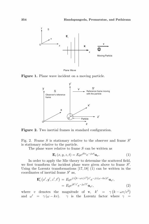
Consider an x-polarized plane wave Ei hitting a small particle moving(relative to an observer in an inertial reference frame [15, 16]) withvelocity v along the z-axis, as shown in Fig. 1.

Consider two inertial frames S and S′ in standard configura-tion [17] with a relative velocity v along the z-axis , as shown in


K

z

v

Plane Wave

Moving Particle

Ei

z

y

x

S

O

Figure 1. Plane wave incident on a moving particle.

v

z'

x'

y'

z

y

x

SS'

O

O’

Observer's reference

frame

Reference frame moving

with the particle

Particle

Figure 2. Two inertial frames in standard configuration.

Fig. 2. Frame S is stationary relative to the observer and frame S′is stationary relative to the particle.

The plane wave relative to frame S can be written as

Ei (x, y, z, t) = E0ejkze−jωtux. (1)

In order to apply the Mie theory to determine the scattered field,we first transform the incident plane wave given above to frame S′.Using the Lorentz transformations [17, 18] (1) can be written in thecoordinates of inertial frame S′ as,

E′i(x′, y′, z′, t′

)= E0e

jγ(k−ωv/c2)z′e−jγ(ω−kv)t′ux′ ,

= E0ejk′z′e−jω′t′ux′ , (2)

where v denotes the magnitude of v, k′ = γ(k − ωv/c2

)and ω′ = γ (ω − kv). γ is the Lorentz factor where γ =


1/(√

1− v2/c2). E′i (x′, y′, z′, t′) is time harmonic and can be expressed

as E′i (x′, y′, z′, t′) = E′i (x

′, y′, z′) e−jγ(ω−kv)t′ .Writing E′i (x

′, y′, z′) in spherical coordinates results in

E′i(x′, y′, z′

)= E0e

jk′r′ cos θ′ux′ , (3)

where ux′ = Sθ′Cφ′ur′ + Cθ′Cφ′uθ′ − Sφ′uφ′ and Sθ′ = sin θ′, Cθ′ =cos θ′, Sφ′ = sinφ′ and Cφ′ = cosφ′. We use this notation throughoutthis paper. We can expand E′i in spherical harmonics as [19],

E′i = E0

∞∑

n=1

jn 2n + 1n(n + 1)

(M(1)

o1n − jN(1)e1n

), (4)

where Mo1n = Cφ′πnzn(ρ)uθ′ − Sφ′τnzn(ρ)uφ′ , Ne1n = Cφ′n(n +1)Sθ′πnzn(ρ)/ρur′+Cφ′τnD[ρzn(ρ)]/ρuθ′−Sφ′πnD[ρzn(ρ)]/ρuφ′ , Ne1n =∇′ ×Me1n/k′, No1n = ∇′ ×Mo1n/k′. Thus, Me1n =−Sφ′πnzn(ρ)uθ′−Cφ′τnzn(ρ)uφ′ , No1n = Sφ′n(n+1)Sθ′πnzn(ρ)/ρu′r +Sφ′τnD[ρzn(ρ)]/ρuθ′ + Cφ′πnD[ρzn(ρ)]/ρuφ′ . Superscripts appendedto the functions M and N denote the kind of the spherical Besselfunction zn: (1) denotes jn(k1r) (i.e., spherical Bessel functions ofthe first kind [20]) and (3) denotes h

(1)n (kr) (i.e., spherical Bessel

functions of the third kind, or spherical Hankel functions [20]). Theangle-dependent functions πn = P 1

n(Cθ′)/Sθ′ and τn = dP 1n(Cθ′)/dθ′

where P 1n are the associate Legendre polynomials of order 1 and de-

gree n. These functions can be computed by upward recurrence us-ing πn = (2n− 1/n− 1)Cθ′πn−1 − (n/n− 1)πn−2, τn = nCθ′πn −(n + 1)πn−1, beginning with π0 = 0 and π1 = 1. ρ = k′r′ and∇′ ≡ ∂/∂x′ux′ + ∂/∂y′uy′ + ∂/∂z′uz′ denotes the gradient operatorwith respect to inertial frame S′. k′1 is the wave number of the waveinside the scatterer (moving particle) and k′ is the wave number ofthe wave outside the scatterer. D represents the first derivative withrespect to ρ. (A complete derivation of the expansion of the electricfield using spherical harmonics can be found in [19]).

From (2) we have ∂/∂t′ ≡ −jω′. Thus, from Maxwell’s equations

∇′ ×E′ = jω′B′,

B′ = −j1ω′∇′ ×E′.

(5)

In frame S′, Minkowski constitutive relations hold. These are given bythe following two equations [21].

D′ +v ×H′

c2− εE′ − εv ×B′ = 0, (6)

B′ − v ×E′

c2− µ0H′ + µ0v ×D′ = 0. (7)


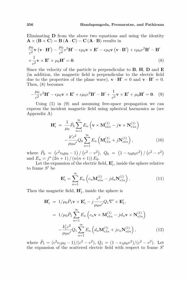
Eliminating D from the above two equations and using the identityA× (B×C) = B (A ·C)−C (A ·B) results inµ0

c2v

(v ·H′)− µ0

c2v2H′ − εµ0v ×E′ − εµ0v

(v ·B′) + εµ0v

2B′ −B′

+1c2

v ×E′ + µ0H′ = 0. (8)

Since the velocity of the particle is perpendicular to B, H, D and E(in addition, the magnetic field is perpendicular to the electric fielddue to the properties of the plane wave), v ·H′ = 0 and v · B′ = 0.Then, (8) becomes

−µ0

c2v2H′ − εµ0v ×E′ + εµ0v

2B′ −B′ +1c2

v ×E′ + µ0H′ = 0. (9)

Using (5) in (9) and assuming free-space propagation we canexpress the incident magnetic field using spherical harmonics as (seeAppendix A)

H′i =

1µ0

P0

∞∑

n=1

En

(v ×M(1)

o1n − jv ×N(1)e1n

)

− k′c2

µ0ω′Q0

∞∑

n=1

En

(M(1)

e1n + jN(1)o1n

), (10)

where P0 =(c2ε0µ0 − 1

)/

(c2 − v2

), Q0 =

(1− ε0µ0v

2)/

(c2 − v2

)and En = jn (2n + 1) / (n(n + 1)) E0.

Let the expansion of the electric field, E′1, inside the sphere relativeto frame S′ be

E′1 =∞∑

n=1

En

(cnM

(1)o1n − jdnN

(1)e1n

). (11)

Then the magnetic field, H′1, inside the sphere is

H′1 = 1/µ0P1v ×E′1 − j

c2

µ0ω′Q1∇′ ×E′1,

= 1/µ0P1

∞∑

n=1

En

(cnv ×M(1)

o1n − jdnv ×N(1)e1n

)

− k′1c2

µ0ω′Q1

∞∑

n=1

En

(dnM

(1)e1n + jcnN

(1)o1n

), (12)

where P1 = (c2ε1µ0 − 1)/(c2 − v2), Q1 = (1− ε1µ0v2)/(c2 − v2). Let

the expansion of the scattered electric field with respect to frame S′


be [19]

E′s =∞∑

n=1

En

(janN

(3)e1n − bnM

(3)o1n

). (13)

Then the scattered magnetic field will be

H′s =

1µ0

P0v ×E′s − jc2

µ0ω′Q0∇′ ×E′s,

=1µ0

P0

∞∑

n=1

En

(janv ×N(3)

e1n − bnv ×M(3)o1n

)

+k′c2

µ0ω′Q0

∞∑

n=1

En

(jbnN

(3)o1n + anM

(3)e1n

). (14)

On the scatterer-medium boundary (i.e., on the surface of thescatterer) we have the following boundary conditions [19](

E′i + E′s −E′1)× ur′ =

(H′

i + H′s −H′

1

)× ur′ = 0. (15)

That is, the tangential components of E′ and H′ are continuous acrossa boundary separating two media of different properties [19]. Theabove boundary conditions can be written in component form as (foreach n)

F′iβ + F′sβ = F′1β, (16)

where F = E,H and β = θ, φ. On the boundary r′ = a where a is theradius of the spherical scatterer. Let χ represents ρ on the boundarywhere χ = k′a, χ1 = k′1a and m = k′1/k′.

Equations (4), (11) and (13) can be written in component formand used in the boundary condition given by (16) to obtain twoequations relating the four scattering coefficients, an, bn, cn and dn

(see Appendix B). Similarly, (10), (12) and (14) can be written incomponent form and used in the boundary condition given by (16)to obtain two equations relating the four scattering coefficients (seeAppendix B). By solving these four equations we obtain the fourscattering coefficients that are required to calculate the Mie solution.

an =ΨΩ

, (17)

bn =Y

Z, (18)

cn =1

MaZ(ZJa −HaY ) , (19)

dn =m

BaΩ(AaΩ− IaΨ) , (20)


where

Ω =(

jP0ΓIa − jP0ΛHa − k′Q0∆Haχ− jP1ΓIa + jP1ΛMaIa

Ba

+k′1Q1∆mχMaIa

Ba

),

Ψ =(

jP0ΓAa − jP0ΛJa − k′Q0∆Jaχ− jP1ΓAa + jP1ΛMaAa

Ba

+k′1Q1∆mχMaAa

Ba

),

Y =(

P0ΓJaχ− jP0XJa − jk′Q0∆Aa + jP0XHaΨΩ− P1ΓJaχ

+jP1XMaAa

Ba− jP1

XMaIa

Ba

ΨΩ

+ jk′1Q1∆BaJa

mMa

),

Z =(

P0ΓHaχ− jk′Q0∆Ia − P1ΓHaχ + jk′1Q1∆BaHa

mMa

),

P0 = v × P0, P1 = v × P1, Π = πn(Cθ′), Ja = jn(χ), Ma = jn(χ1) =jn(mχ), Aa = D[χjn(χ)] = (d/dχ) [χjn(χ)], Ba = D[χ1jn(χ1)] =D[mχjn(mχ)] = (d/dχ) [mχjn(mχ)], T = τn(Cθ′), Ha = h

(1)n (χ),

Ia = D[χh(1)n (χ)], Γ = Cθ′(Π×Π−T ×T ), ∆ = c2/ω′(Π×Π−T ×T ),

Λ = n(n + 1)S2θ′Π× T and X = n(n + 1)S2

θ′Π×Π.Thus, we have calculated the scattering coefficients an, bn, cn and

dn. Hence, the scattered field and the field inside the scatterer areknown with respect to frame S′. We then need to transform thesefields to reference frame S, which is stationary relative to the observer.We first write the field components with respect to the Cartesiancoordinate system and then use the standard field transformations fromframe S′ to frame S.

The Cartesian field components can be constructed from thespherical field components using the following transformations

F ′x = F ′

rSθ′Cφ′ + FθCθ′Cφ′ − F ′φSφ′ , (21)

F ′y = F ′

rSθ′Sφ′ + F ′θCθ′Sφ′ + F ′

φCφ′ , (22)

F ′z = F ′

rCθ′ − F ′θSθ′ , (23)

where F = E, H.Using the expression for the scattered electric field (i.e., (13)) in

(21) to (23), we obtain the Cartesian components of the electric field


as

E′s,x =

∞∑

n=1

En

[jan

(N

(3)e1n,rSθ′Cφ′ + N

(3)e1n,θCθ′Cφ′ −N

(3)e1n,φSφ′

)

−bn

(M

(3)o1n,θCθ′Cφ′ −M

(3)o1n,φSφ′

)], (24)

E′s,y =

∞∑

n=1

En

[jan

(N

(3)e1n,rSθ′Sφ′ + N

(3)e1n,θCθ′Sφ′ + N

(3)e1n,φCφ′

)

−bn

(M

(3)o1n,θCθ′Sφ′ + M

(3)o1n,φCφ′

)], (25)

E′s,z =

∞∑

n=1

En

[jan

(N

(3)e1n,rCθ′ −N

(3)e1n,θSφ′

)+ bnM

(3)o1n,θSθ′

]. (26)

Similarly, using the expression for the scattered magnetic field(i.e., (14)) in (21) to (23), we obtain the Cartesian components of themagnetic field as,

H ′s,x =

P0

µ0

∞∑

n=1

En

[jan

(−N

(3)e1n,φCφ′ −N

(3)e1n,θCθ′Sφ′ −N

(3)e1n,rSθ′Sφ′

)

+bn

(M

(3)o1n,φCφ′ + M

(3)o1n,θCθ′Sφ′

)]

+k′c2

µ0ω′Q0

∞∑

n=1

En

[jbn

(N

(3)o1n,rSθ′Cφ′+N

(3)o1n,θCθ′Cφ′−N

(3)o1n,φSφ′

)

an

(M

(3)e1n,θCθ′Cφ′ −M

(3)e1n,φSφ′

)], (27)

H ′s,y =

P0

µ0

∞∑

n=1

En

[jan

(−N

(3)e1n,φSφ′ + N

(3)e1n,θCθ′Cφ′ + N

(3)e1n,rSθ′Cφ′

)

+bn

(M

(3)o1n,φSφ′ −M

(3)o1n,θCθ′Cφ′

)]

+k′c2

µ0ω′Q0

∞∑

n=1

En

[jbn

(N

(3)o1n,rSφ′Sθ′+N

(3)o1n,θCθ′Sφ′+N

(3)o1n,φCφ′

)

+an

(M

(3)e1n,θCθ′Sφ′ + M

(3)e1n,φCφ′

)], (28)


H ′s,z=

P0

µ0

∞∑

n=1

En

[− jan

(N

(3)e1n,φSθ′Cθ′ + N

(3)e1n,θCθ′Sθ′ + N

(3)e1n,rS

2θ′

)

+bn

(M

(3)o1n,φSθ′Cθ′ + M

(3)o1n,θCθ′Sθ′

) ]

+k′c2

µ0ω′Q0

∞∑

n=1

En

[jbn

(N

(3)o1n,rCθ′−N

(3)o1n,φSθ′

)−anM

(3)e1n,φSθ′

], (29)

where P0 = v × P0.These components of the scattered electromagnetic field with

respect to frame S′ should then be transformed back to the inertialreference frame S of the observer. Using the Minkowski constitutiverelations [21] in the standard field transformation equations [22] weobtain the following field transformations between the two inertialframes (see Appendix C)

Ex = γ

(E′

x +v

cµ0L1L2H

′y +

v2

cL1L3E

′x

), (30)

Ey = γ

(E′

y −v

cµ0L1L2H

′x +

v2

cL1L3E

′y

), (31)

Ez = E′z, (32)

Hx = γ

(L1L2H

′x −

v

µ0L1L3E

′y −

v

µ0cE′

y

), (33)

Hy = γ

(L1L2H

′y +

v

µ0L1L3E

′x +

v

µ0cE′

x

), (34)

Hz = L1L2H′z, (35)

where L1 = 1/(1− ε0µ0v2), L2 = 1− (v2/c2) and L3 = 1/c2 − ε0µ0.

Hence, using (24) to (26) and (27) to (29) in (30) to (35), wecan calculate all the components of electric and magnetic fields withrespect to inertial frame S.

2.2. Moving Source and Stationary Particle

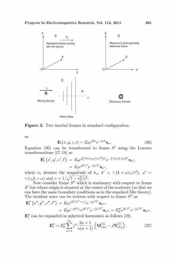
Consider a source moving with a velocity vs along the z-axis, relative toan observer. The source is emitting x-polarized plane waves Ei whichhit a small stationary particle (relative to the observer), as shown inFig. 3. Consider two inertial frames S and S′ in standard configurationwith a relative velocity vs. Frame S is stationary relative to the sourceand frame S′ is stationary relative to the particle and the observer, asshown in Fig. 3. The plane wave with respect to frame S can be written


z'

x'

y’

z

y

x

S S'vs

O O’


with the source

Observer’s (and particle’s)

reference frame

K

z’

vs

Plane Wave

Stationary Particle

Ei

Moving Source


asEi(x, y, z, t) = E0e

jkze−jωtux. (36)Equation (36) can be transformed to frame S′ using the Lorentztransformations [17, 18] as

E′i(x′, y′, z′, t′

)= E0e

j(γk+vsωγ/c2)z′e−jγ(vsk+ω)t′ux′ ,

= E0ejk′z′e−jω′t′ux′ ,

where vs denotes the magnitude of vs, k′ = γ(k + ωvs/c2

), ω′ =

γ (vsk + ω) and γ = 1/√

1− v2s/c2.

Now consider frame S′′ which is stationary with respect to frameS′ but whose origin is situated at the centre of the scatterer (so that wecan have the same boundary conditions as in the standard Mie theory).The incident wave can be written with respect to frame S′′ as

E′′i(x′′, y′′, z′′, t′′

)= E0e

jk′(z′′−cz)e−jω′t′′ux′′ ,

= E0e−jk′czejk′z′′e−jω′t′′ux′′ , = E′′

0ejk′z′′e−jω′t′′ux′′ .

E′′i can be expanded in spherical harmonics as follows [19].

E′′i = E′′0

∞∑

n=1

jn 2n + 1n(n + 1)

(M(1)

o1n − jN(1)e1n

). (37)


From Maxwell’s equations

B′′ = −j1ω′∇′′ ×E′′. (38)

In frame S′′ the following relation holds:

B′′ = µ0H′′. (39)

Using (39) and (37) in (38), for the incident magnetic field, we get

H′′i = − k′

µ0ω′

∞∑

n=1

E′′n

(M(1)

e1n + jN(1)o1n

). (40)

From the format of (37) and (40) it is evident that we can obtain thescattered field by replacing k by k′, ω by ω′ and En by E′′

n in the resultsof the standard Mie theory (which is derived for a stationary sourceand a stationary particle). Thus, the scattered field is

E′′s =∞∑

n=1

E′′n

(janN

(3)e1n − bnM

(3)o1n

),

H′′s =

k′

ω′µ0

∞∑

n=1

E′′n

(jbnN

(3)o1n + anM

(3)e1n

),

where

an =m2jn(mχ)D[χjn(χ)]− jn(χ)D[mχjn(mχ)]

m2jn(mχ)D[χh(1)n (χ)]− h

(1)n (χ)D[mχjn(mχ)]

,

bn =jn(mχ)D[χjn(χ)]− jn(χ)D[mχjn(mχ)]

jn(mχ)D[χh(1)n (χ)]− h


,

and χ = k′a, m = k′1/k′.

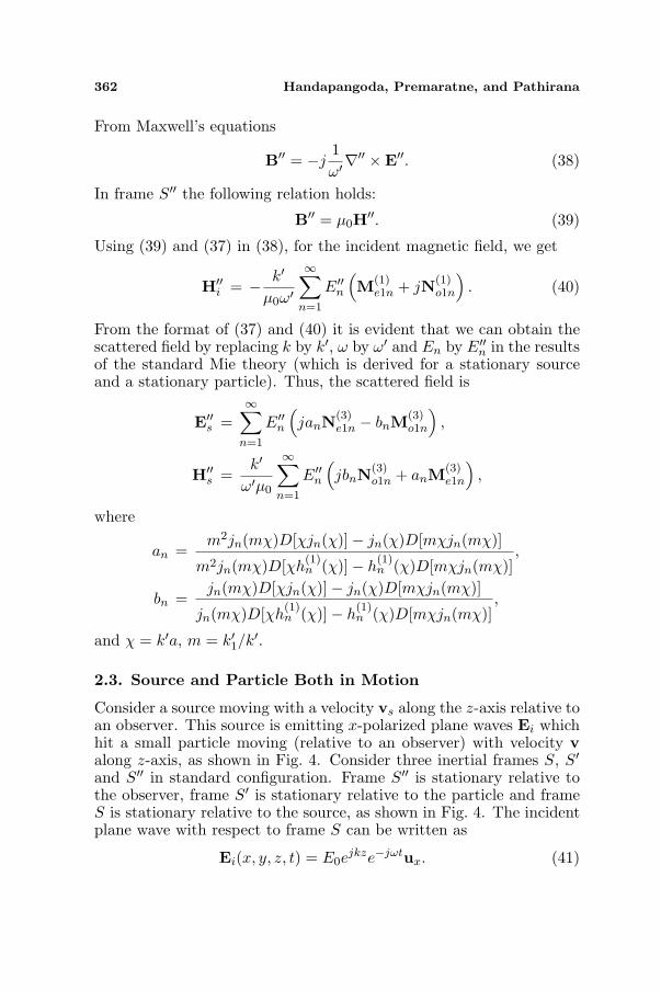
2.3. Source and Particle Both in Motion

Consider a source moving with a velocity vs along the z-axis relative toan observer. This source is emitting x-polarized plane waves Ei whichhit a small particle moving (relative to an observer) with velocity valong z-axis, as shown in Fig. 4. Consider three inertial frames S, S′and S′′ in standard configuration. Frame S′′ is stationary relative tothe observer, frame S′ is stationary relative to the particle and frameS is stationary relative to the source, as shown in Fig. 4. The incidentplane wave with respect to frame S can be written as

Ei(x, y, z, t) = E0ejkze−jωtux. (41)


z’

x’

y’

z

y

x

vs v

z''

x''

y’’

O O’’ O’


with the sourceObserver’s reference

frameReference frame moving

with the particle

K

z''

vs

Plane Wave

Moving Particle

Ei

Moving Source

v

S S'' S'


Equation (41) can be transformed to frame S′′ as

E′′i (x′′, y′′, z′′, t′′) = E0e

jγ1(k+vsω/c2)z′′e−jγ1(ω+vsk)t′′ux′′ ,

= E0ejk′′z′′e−jω′′t′′ux′′ , (42)

where k′′ = γ1

(k + vsω/c2

), ω′′ = γ1 (ω + vsk) and γ1 =

1/√

1− v2s/c2. Equation (42) can then be transformed to frame S′

asE′i(x

′, y′, z′, t′) = E0ejγ2(k′′−vω′′/c2)z′e−jγ2(ω′′−vk′′)t′ux′ ,

= E0ejk′z′e−jω′t′ux′ ,

where k′ = γ2

(k′′ − vω′′/c2

)= γ1γ2

((1− vsv/c2

)k +

(vs/c2 − v/c2

)ω),

ω′ = γ2 (ω′′ − vk′′) = γ1γ2

((1− vsv/c2

)ω + (vs − v) k

)and γ2 =

1/√

1− v2/c2 ·E′i can be expanded using spherical harmonics as

E′i = E0

∞∑

n=1

jn 2n + 1n(n + 1)

(M(1)

o1n − jN(1)e1n

). (43)

From Maxwell’s equations

B′ = −j1ω′∇′ ×E′. (44)


In frame S′ Minkowski constitutive relations hold. Using (44), (6) and(7), we get

H′ =1µ0

Pv ×E′ − jc2

µ0ω′Q∇′ ×E′, (45)

where P =(c2εµ0 − 1

)/

(c2 − v2

)and Q =

(1− εµ0v

2)/

(c2 − v2

).

Using (43) in (45) we get

H′i =

1µ0

P0

∞∑

n=1

En

(v ×M(1)


)

− k′c2

µ0ω′Q0

∞∑

n=1

En

(M(1)

e1n + jN(1)o1n

). (46)

Equations (43) and (46) are exactly similar to (4) and (10).Therefore, following a similar argument (and using the same boundaryconditions) as in Section 2.1, we can determine the scattered fieldrelative to frame S′. In addition, the Cartesian components of electricand magnetic fields relative to frame S′ can be obtained using (24) to(26) and (27) to (29). Since the observer is stationary relative to frameS′′, we should convert these fields to frame S′′. Using the Minkowskiconstitutive relations [21] in the standard field transformations [22], weobtain the scattered field as seen by the observer using the followingtransformations

E′′x = γ2

(E′

x +v

cµ0L1L2H

′y +

v2

cL1L3E

′x

), (47)

E′′y = γ2

(E′

y −v

cµ0L1L2H

′x +

v2

cL1L3E

′y

), (48)

E′′z = E′

z, (49)

H ′′x = γ2

(L1L2H

′x −

v

µ0L1L3E

′y −

v

µ0cE′

y

), (50)

H ′′y = γ2

(L1L2H

′y +

v

µ0L1L3E

′x +

v

µ0cE′

x

), (51)

H ′′z = L1L2H

′z. (52)

where L1 = 1/(1− εµ0v2), L2 = 1− (v2/c2) and L3 = 1/c2 − εµ0.

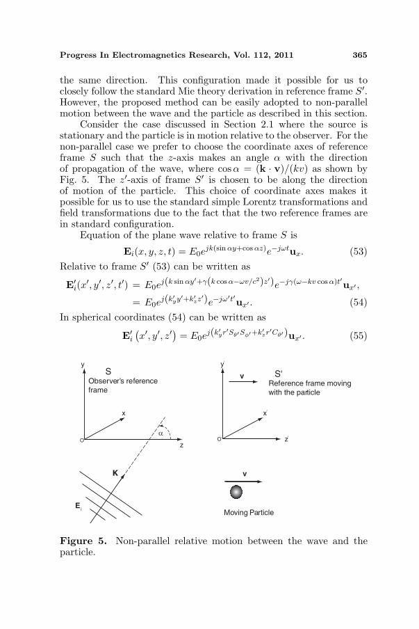
2.4. Non-parallel Motion between the Wave and the Particle

In all the three cases discussed in the previous three sections, we haveconsidered the relative motion of the plane wave and the particle in


the same direction. This configuration made it possible for us toclosely follow the standard Mie theory derivation in reference frame S′.However, the proposed method can be easily adopted to non-parallelmotion between the wave and the particle as described in this section.

Consider the case discussed in Section 2.1 where the source isstationary and the particle is in motion relative to the observer. For thenon-parallel case we prefer to choose the coordinate axes of referenceframe S such that the z-axis makes an angle α with the directionof propagation of the wave, where cosα = (k · v)/(kv) as shown byFig. 5. The z′-axis of frame S′ is chosen to be along the directionof motion of the particle. This choice of coordinate axes makes itpossible for us to use the standard simple Lorentz transformations andfield transformations due to the fact that the two reference frames arein standard configuration.

Equation of the plane wave relative to frame S is

Ei(x, y, z, t) = E0ejk(sin αy+cos αz)e−jωtux. (53)

Relative to frame S′ (53) can be written as

E′i(x′, y′, z′, t′) = E0e

j(k sin αy′+γ(k cos α−ωv/c2)z′)e−jγ(ω−kv cos α)t′ux′ ,

= E0ej(k′yy′+k′zz′)e−jω′t′ux′ . (54)

In spherical coordinates (54) can be written as

E′i(x′, y′, z′

)= E0e

j(k′yr′Sθ′Sφ′+k′zr′Cθ′)ux′ . (55)

v

z’

x’

y’

z

y

x

O O’

Observer’s reference

frameReference frame moving

with the particle

K

Ei

α

v

Moving Particle

S S'

Figure 5. Non-parallel relative motion between the wave and theparticle.


The next step is to expand the plane wave in spherical harmonics.

E′i =∞∑

n=1

(Bo1nM

(1)o1n + Ae1nN

(1)e1n

). (56)

The form of (55) is different to that of (3) of Section 2.1. Theform of the transformed equation of the plane wave in Section 2.1 issimilar to that of the standard Mie theory and therefore the sphericalharmonic expansion coefficients Bo1n and Ae1n were equal to those ofthe standard Mie theory. (i.e., Bo1n = jnE0(2n + 1)/(n(n + 1)) andAe1n = −jE0j

n(2n + 1)/(n(n + 1))). However, for the non-parallelcase these coefficients will not be the same and the integrals involvedin the determination of these coefficients are much more complicatedthan those involved in the parallel motion case. Nevertheless, oncethese coefficients are evaluated, the scattered field can be obtainedusing the method discussed in Section 2.1. That is, once Bo1n andAe1n are evaluated, the same steps and field transformations can beused to determine the scattered field relative to the observer.

3. VALIDATION OF THE SCATTERING THEORYRESULTS

In this section, we carryout two tests to validate the results of theproposed theory. First, we show that the expressions derived for aplane wave scattering by a moving particle reduces to those of thestandard Mie theory when the relative velocity is set to zero. Second,we show that when the refractive index of the particle is equal to thatof the medium, no scattering takes place, as expected, and the fieldexperienced by an observer moving with the particle is the same asthat predicted by the relativistic Doppler formula [23].

3.1. Reduction to Standard Mie Theory When the RelativeVelocity is Zero

Consider setting the relative velocity v to zero in the problem discussedin Section 2.1 so that the particle is stationary relative to the observer.Transformations given by (30) to (35) then reduce to

Ex = γE′x, (57)

Ey = γE′y, (58)

Ez = E′z, (59)

Hx = γL1L2H′x, (60)

Hy = γL1L2H′y, (61)


Hz = L1L2H′z. (62)

In addition, when v = 0, γ = 1, L1 = 1 and L2 = 1. Therefore, (57)to (62) further reduce to

Fn = F ′n, (63)

where F = E, H and n = x, y, z. Thus, when v = 0

E = E′, (64)H = H′. (65)

It is also evident that in this special case the two inertial referenceframes S and S′ are the same and thus the spherical harmonics M andN would remain unchanged. Using (13) and (14) in (64) and (65) withv = 0, for the scattered field with respect to frame S when the particleis stationary, we get

Es =∞∑

n=1

En

(janN

(3)e1n − bnM

(3)o1n

), (66)

Hs =k′c2

µ0ω′Q

∞∑

n=1

En

(jbnN

(3)o1n + anM

(3)e1n

). (67)

Q =(1− εµ0v

2)/

(c2 − v2

). (68)

With respect to frame S, εµ0 = 1/c2. Hence,

Q =(1− v2/c2

)/

(c2 − v2

)= 1/c2.

When v = 0, k′ = k and ω′ = ω. Equation (67) thus reduces to

Hs =k

µ0ω

∞∑

n=1

En

(jbnN

(3)o1n + anM

(3)e1n

). (69)

Using a similar argument for the field inside the scatterer, we get

E1 =∞∑

n=1

En

(cnM

(1)o1n − jdnN

(1)e1n

), (70)

H1 = − k1

µ0ω

∞∑

n=1

En

(dnM

(1)e1n + jcnN

(1)o1n

). (71)

Thus, it is evident from (66), (69), (70) and (71) that the expressionsfor the scattered electric and magnetic fields have reduced to thestandard expressions (of Mie theory), given that the expressions forcoefficients an, bn, cn and dn reduce to the standard expressions whenv is set to zero.


3.1.1. Reduction of Scattering Coefficients When the Particle isStationary

When v = 0, P0 = 0 and P1 = 0. In addition, k′ = k and k′1 = k1.Hence (17) reduces to

an =m2MaAa−JaBa

m2MaIa−HaBa

=m2jn(mχ)D[χjn(χ)]−jn(χ)D[mχjn(mχ)]

m2jn(mχ)D[χh(1)n (χ)]−h


. (72)

Equation (18) reduces to

bn =MaAa−JaBa

MaIa−HaBa=

jn(mχ)D[χjn(χ)]−jn(χ)D[mχjn(mχ)]

jn(mχ)D[χh(1)n (χ)]−h


. (73)


cn =JaIa−HaAa

MaIa−HaBa=

jn(χ)D[χh(1)n (χ)]− h

(1)n D[χjn(χ)]

jn(mχ)D[χh(1)n (χ)]− h


. (74)


dn =mJaIa −mHaAa

m2MaIa −HaBa

=mjn(χ)D[χh

(1)n (χ)]−mh

(1)n (χ)D[χjn(χ)]

m2jn(mχ)D[χh(1)n (χ)]− h


. (75)

Equations (66), (69), (70) and (71) together with (72) to (75) are theexpressions for the scattered field of a plane wave scattered by a smallstationary spherical particle [19]. Thus, the modified theory for themoving particle has been reduced to the standard Mie theory whenthe velocity of the particle is set to zero.

In the problem of moving source and stationary particle (relativeto the observer) discussed in Section 2.2, when the relative velocity vs

is set to zero, γ = 1, k′ = k and ω′ = ω. Hence, the problem reducesto the standard Mie scattering problem.

In the problem where both the source and the particle are inmotion, as discussed in Section 2.3, when vs and v is set to zero,γ1 = 1, γ2 = 1, k′ = k and ω′ = ω. In addition, in the transformationsof the field given by (47) to (52), L1 = 1 and L2 = 1. Then, thosefield transformations reduce to the same form as in (63). Therefore,using the same argument as for the case of the stationary source andthe moving particle, we have the expressions reduced to those of thestandard Mie theory when vs = v = 0.


3.2. Comparison with Doppler Shift Formula

In this section, we show that the proposed formulation is comparablewith the Doppler shift formula. We consider a particle with the samerefractive index as that of the medium so that no scattering takes placeand the whole system behaves as if there is a non-scattering objectpresent. We show that, in this scenario, no scattering takes place andthe field inside the particle is equal to the incident field. In addition, weshow that an observer moving with the particle experiences a frequencyshift of the plane wave equal to that predicted by the Doppler shiftformula, as expected. For this comparison, we consider the casediscussed in Section 2.1, where the source is stationary while theparticle is in motion.

When the refractive index of the particle is equal to that of themedium, ε1 = ε0. Then in (17) to (20), k′1 = k′, m = 1, Q1 = Q0 andP1 = P0. In addition, since ρ1 = ρ, χ1 = χ, Ba = Aa and Ma = Ja

(see Appendix B). Then,

Ψ =(

jP0ΓAa − jP0ΛJa − k′Q0∆Jaχ− jP0ΓAa + jP0ΛJaAa

Aa

+k′Q0∆χJaAa

Aa

)= 0.

Ω =(

jP0ΓIa − jP0ΛHa − k′Q0∆Haχ− jP0ΓIa + jP0ΛJaIa

Aa

+k′Q0∆χJaIa

Aa

)=

(jP0Λ + k′Q0∆χ

) (JaIa

Aa−Ha

)6= 0.

Therefore,

an = Ψ/Ω = 0.

Y =(


+jP0XJaAa

Aa− jP0

XJaIa

Aa

ΨΩ

+ jk′Q0∆AaJa

Ja

)= 0.

Z =(

P0ΓHaχ− jk′Q0∆Ia − P0ΓHaχ + jk′Q0∆AaHa

Ja

)

= jk′Q0∆(

AaHa

Ja− Ia

)6= 0.

Therefore,

bn = Y/Z = 0.


Then,cn = 1/Ja (Ja −Habn) = 1,

dn = 1/Aa (Aa − Iaan) = 1.

Using an and bn in (13) and (14), for the scattered field with respectto frame S′, we get

E′s = 0,

H′s = 0.

Using cn and dn in (11) and (12) (and combining the time dependencyterm), for the field inside the particle with respect to frame S′, we get

E′1(x′, y′, z′, t′

)=

∞∑

n=1

En

(M(1)

o1n − jN(1)e1n

)e−jω′t′ ,

= E′i(x′, y′, z′

)e−jω′t′

H′1

(x′, y′, z′, t′

)=

[1µ0

P0

∞∑

n=1

En

(v ×M(1)


)

− k′c2

µ0ω′Q0

∞∑

n=1

En

(M(1)

e1n + jN(1)o1n

)]e−jω′t′ ,

= H′i

(x′, y′, z′

)e−jω′t′ .

From (2)ω′ = γ(ω − kv) = γ (ω − ωv/vp) ,

=c√

c2 − v2(1− v/vp) ω,

where v is the speed of the observer, ω is the angular frequency of theplane wave relative to the medium and vp is the phase velocity of theplane wave relative to the medium.

Thus, when the refractive index of the particle is equal to thatof the medium, there is no scattered field, while the field inside theparticle, as seen by an observer moving with the particle, is equalto the incident field in magnitude, but the frequency is shifted by theamount predicted by the special relativistic Doppler formula [23]. Thisshows that the derived formula is well-behaved even under the limitingconditions, making it widely usable for both strong and weak scatteringscenarios.

4. NUMERICAL RESULTS AND DISCUSSION

In this section we present some numerical results that were obtainedby simulating the proposed derivation.


(a) (b)

Figure 6. Distribution of the z-component of the Poynting vectorwithin the xy-plane when the particle is stationary. (a) At z = −a(plane for incoming radiation), (b) at z = a (plane for outgoingradiation).

(a) v=0 (b) v=10 m.s

(c) v=1000 m.s (d) v=0.5× c

−1

−1

Figure 7. Distribution of the z-component of the Poynting vectorwithin the xz-plane for different velocities.


Figure 6 shows the distribution of the z-component of the Poyntingvector within the xy-plane at z = −a and z = a planes, when v is setto zero (i.e., the particle is stationary). For this figure we have set thesimulation parameters to those used for Fig. 4 of [24]. In [24], Wanget al. obtained Fig. 4 using the classical Mie theory. Hence, Fig. 6illustrates that the theory proposed in this paper produces the resultsof the classical Mie theory when the velocity of the particle is set tozero.

Figure 7 shows the distribution of the z-component of the Poyntingvector within the xz-plane, around the particle, for different velocities.For this simulation we have set E0 = 1 V/m, a/λ = 3/4π and anon-magnetic particle with relative permittivity 12 was considered.Figs. 7(a), 7(b), 7(c) and 7(d) were obtained for v = 0, v = 10 m · s−1,v = 1000 m · s−1 and v = 0.5 times the speed of light, respectively.Hence, Fig. 7 illustrates the versatility of the proposed theory, whichis accurate from very low to very high velocities. A comparison ofFigs. 7(a) and 7(b) shows that the standard Mie theory is not a goodapproximation even at very low speeds, such as 10m · s−1.

5. CONCLUSION

In this paper, we addressed the problem of electromagnetic scatteringby particles involving relative motion between the source and theparticle. The proposed technique involves first transforming theproblem to a reference frame co-moving with the particle using theLorentz transformations. Then the Mie theory is applied relativeto this frame. We have closely followed the steps of the standardderivation and obtained the scattered field relative to the referenceframe co-moving with the particle. Field transformations were thenused to transform this field to the reference frame of the observer.When the velocity of the particle and the source were set to zerorelative to the observer, the results reduced to those of the standardMie theory. Using simulations we showed that the standard Mietheory is not a good approximation even at very low speeds such as10m·s−1. By assuming that the refractive index of the particle is equalto that of the medium, we showed that the results of the derivationare compatible with the relativistic Doppler formula.

APPENDIX A. EXPANSION OF THE MAGNETICFIELD USING SPHERICAL HARMONICS

Here, we show how to express the magnetic field in terms of sphericalharmonics using the expression for the electric field.


Using (5) in (9) and simplifying, we get

H′ =1µ0

(c2εµ0 − 1c2 − v2

)v ×E′ − j

c2

µ0ω′

(1− εµ0v

2

c2 − v2

)∇′ ×E′,

=1µ0

Pv ×E′ − jc2

µ0ω′Q∇′ ×E′, (A1)

where P =(c2εµ0 − 1

)/

(c2 − v2

)and Q =

(1− εµ0v

2)/

(c2 − v2

).

We then replace the terms v×E′ and∇′×E′ using spherical harmonics.

v ×E′i =∞∑

n=1

En

[v ×M(1)


], (A2)

∇′ ×E′i = −jk′∞∑

n=1

En

(M(1)

e1n + jN(1)o1n

), (A3)

where En = jn (2n + 1) / (n(n + 1))E0.The velocity v can be decomposed into components as v = vuz′ =

vCθ′ur′ − vSθ′uθ′ . Using (A2) and (A3) in (A1) the incident magneticfield can be written using spherical harmonics as

H′i =

1µ0

P0

∞∑

n=1

En

(v ×M(1)


)

− k′c2

µ0ω′Q0

∞∑

n=1

En

(M(1)

e1n + jN(1)o1n

).

APPENDIX B. SOLUTION FOR THE SCATTERINGCOEFFICIENTS

Here, we present a detailed solution procedure for obtaining thescattering coefficients from the boundary conditions, as mentioned inSection 2.1.

Let Π = πn(Cθ′), J = jn(ρ), M = jn(ρ1) = jn(mρ),A = D[ρjn(ρ)] = d

dρ [ρjn(ρ)], B = D[ρ1jn(ρ1)] = D[mρjn(mρ)] =ddρ [mρjn(mρ)], T = τn(Cθ′), H = h

(1)n (ρ), I = D[ρh

(1)n (ρ)], and let

us use the subscript a assigned to the above notation to denote theevaluation of those functions on the boundary, where r′ = a and henceρ = χ = k′a and ρ1 = χ1 = k′1a. (e.g., Ja = jn(χ) = jn(k′a) where asJ = jn(ρ) = jn(k′r′)).

Using F = E and β = θ in the boundary condition given by (16)we get,

ΠJa − jTAa

χ+ janT

Ia

χ− bnΠHa − cnΠMa + jdnT

Ba

mχ= 0. (B1)


Using F = E and β = φ in the boundary condition given by (16), weget,

−TJa + jΠAa

χ− janΠ

Ia

χ+ bnTHa + cnTMa − jdnΠ

Ba

mχ= 0. (B2)

Using F = H and β = θ in the boundary condition given by (16), weget,

P0Cθ′TJa − jP0Cθ′ΠAa

χ+

k′c2

ω′Q0ΠJa − j

k′c2

ω′Q0T

Aa

χ

+jP0anCθ′ΠIa

χ− P0bnCθ′THa + j

k′c2

ω′Q0bnT

Ia

χ− k′c2

ω′Q0anΠHa

−P1cnCθ′TMa + jP1dnCθ′ΠBa

mχ− k′1c

2

ω′Q1dnΠMa

+jk′1c

2

ω′Q1cnT

Ba

mχ= 0. (B3)

Using F = H and β = φ in the boundary condition given by (16), weget,

P0Cθ′ΠJa − jP0Cθ′TAa

χ− jP0n(n + 1)S2

θ′ΠJa

χ+

k′c2

ω′Q0TJa

−jk′c2

ω′Q0Π

Aa

χ+ jP0anCθ′T

Ia

χ+ jP0ann(n + 1)S2

θ′ΠHa

χ

−P0bnCθ′ΠHa + jk′c2

ω′Q0bnΠ

Ia

χ− k′c2

ω′anQ0THa − P1cnCθ′ΠMa

+jP1dnCθ′TBa

mχ+ jP1dnn(n + 1)S2

θ′ΠMa

mχ− k′1c

2

ω′Q1dnTMa

+jk′1c

2

ω′Q1cnΠ

Ba

mχ= 0 (B4)

Multiplying (B1) by T and (B2) by Π and adding the two resultingequations we get

mIaan + Badn = mAa. (B5)

Multiplying (B1) by Π, multiplying (B2) by T and adding the resultingtwo equations, we get

Macn + Habn = Ja. (B6)

Multiplying (B3) by T , multiplying (B4) by Π and taking the difference


of the resulting two equations, we get

−P0Cθ′Ja(ΠΠ− TT ) + jP0n(n + 1)S2θ′ΠΠ

Ja

χ

+jk′c2

ω′Q0

Aa

χ(ΠΠ− TT )− jP0ann(n + 1)S2

θ′ΠΠHa

χ

+P0bnCθ′Ha(ΠΠ− TT )− jk′c2

ω′Q0bn

Ia

χ(ΠΠ− TT )

+P1cnCθ′Ma(ΠΠ− TT )− jP1dnn(n + 1)S2θ′ΠΠ

Ma

mχ

−jk′1c

2

ω′cnQ1

Ba

mχ(ΠΠ− TT ) = 0. (B7)

where ΠΠ = Π×Π, TT = T × T . Multiplying (B3) by Π, multiplying(B4) by T and taking the difference of the resulting two equations, weget

−jP0Cθ′Aa

χ(ΠΠ− TT ) + jP0n(n + 1)S2

θ′ΠTJa

χ

+k′c2

ω′Q0Ja(ΠΠ− TT ) + jP0anCθ′

Ia

χ(ΠΠ− TT )

−jP0ann(n + 1)S2θ′TΠ

Ha

χ− k′c2

ω′Q0anHa(ΠΠ− TT )

+jP1dnCθ′Ba

mχ(ΠΠ− TT )− jP1dnn(n + 1)S2

θ′TΠMa

mχ

−k′1c2

ω′Q1dnMa(ΠΠ− TT ) = 0. (B8)

Let Γ = Cθ′(ΠΠ − TT ), ∆ = c2

ω′ (ΠΠ − TT ), Λ = n(n + 1)S2θ′ΠT ,

X = n(n + 1)S2θ′ΠΠ. Using (B5) in (B8) (i.e., substituting for dn in

terms of an), we get

an =ΨΩ

, (B9)

where

Ω =(

jP0ΓIa − jP0ΛHa − k′Q0∆Haχ− jP1ΓIa + jP1ΛMaIa

Ba

+k′1Q1∆mχMaIa

Ba

),


Ψ =(

jP0ΓAa − jP0ΛJa − k′Q0∆Jaχ− jP1ΓAa + jP1ΛMaAa

Ba

+k′1Q1∆mχMaAa

Ba

).

Using (B9) in (B5) we get

dn =m

Ba

(Aa − IaΨ

Ω

). (B10)

Using (B6), (B9) and (B10) in (B7), we get

bn =Y

Z,

where

Y =(


+jP1XMaAa

Ba− jP1

XMaIa

Ba

ΨΩ

+ jk′1Q1∆BaJa

mMa

),

Z =(

P0ΓHaχ− jk′Q0∆Ia − P1ΓHaχ + jk′1Q1∆BaHa

mMa

).

Then

cn =1

Ma

(Ja −Ha

Y

Z

).

APPENDIX C. FIELD TRANSFORMATIONS BETWEENFRAMES S AND S′

Here we show how the Cartesian field components of inertial frame S′are transformed to those of inertial frame S.

The electromagnetic field transformations between the two inertialreference frames S and S′, which are in standard configuration, aregiven by [22]

Ex = γ(E′

x +v

cB′

y

),

Ey = γ(E′

y −v

cB′

x

),

Ez = E′z,

Bx = γ(B′

x −v

cE′

y

),

By = γ(B′

y +v

cE′

x

),

Bz = B′z.


From Minkowski constitutive relations (i.e., from (6) and (7)) we candetermine B′ from E′ and H′ as follows.

B′=1

1− εµ0v2

(−µ0v

2

c2H′−εµ0v ×E′+

1c2

v ×E′+µ0H′)

. (C1)

v ×E′=−vE′yux′ + vE′

xuy′ . (C2)

Using (C2) in (C1), for the x, y and z-components of magnetic fluxdensity with respect to frame S′ we have,

B′x =

11− εµ0v2

(µ0

(1− v2

c2

)H ′

x − v

(1c2− εµ0

)E′

y

),

B′y =

11− εµ0v2

(µ0

(1− v2

c2

)H ′

y + v

(1c2− εµ0

)E′

x

),

B′z =

11− εµ0v2

µ0

(1− v2

c2

)H ′

z.

Therefore, the electromagnetic field transformations can be written as

Ex = γ

(E′

x +v

cµ0L1L2H

′y +

v2

cL1L3E

′x

),

Ey = γ

(E′

y −v

cµ0L1L2H

′x +

v2

cL1L3E

′y

),

Ez = E′z,

Hx = γ

(L1L2H

′x −

v

µ0L1L3E

′y −

v

µ0cE′

y

),

Hy = γ

(L1L2H

′y +

v

µ0L1L3E

′x +

v

µ0cE′

x

),

Hz = L1L2H′z,

where L1 = 1/(1− εµ0v2), L2 = 1− (v2/c2) and L3 = 1/c2 − εµ0.

REFERENCES

1. Shiozawa, T., “Electromagnetic scattering by a moving smallparticle,” J. Appl. Phys., Vol. 39, 2993–2997, 1968.

2. Reid, J. P. and L. Mitchem, “Laser probing of single-aerosoldroplet dynamics,” Annu. Rev. Phys. Chem., Vol. 57, 245–271,2006.

3. Konig, G., K. Anders, and A. Frohn, “A new light-scatteringtechnique to measure the diameter of periodically generatedmoving droplets,” J. Aerosol. Sci., Vol. 17, 157–167, 1986.


4. Beuthan, J., O. Minet, J. Helfmann, M. Herrig, and G. Muller,“The spatial variation of the refractive index in biological cells,”Phys. Med. Biol., Vol. 41, 369–382, 1996.

5. Kelly, K. L., E. Coronado, L. L. Zhao, and G. C. Schatz, “Theoptical properties of metal nanoparticles: The influence of size,shape and dielectric environment,” J. Phys. Chem. B, Vol. 107,668–677, 2003.

6. Quinten, M. and J. Rostalski, “Lorenz-Mie theory for spheresimmersed in an absorbing host medium,” Part. Part. Syst.Charact., Vol. 13, 89–96, 1996.

7. Gouesbet, G., “Generalized Lorenz-Mie theory and applications,”Part. Part. Syst. Charact., Vol. 11, 22–34, 1994.

8. Purcell, E. M. and C. R. Pennypacker, “Scattering and absorptionof light by nonspherical dielectric grains,” The Astrophys. J.,Vol. 186, 705–714, 1973.

9. Acquista, C., “Validity of modifying Mie theory to describescattering by nonspherical particles,” Appl. Opt., Vol. 17, 3851–3852, 1978.

10. Censor, D., “Non-relativistic scattering in the presence of movingobjects: The Mie problem for a moving sphere,” Progress InElectromagnetics Research, Vol. 46, 1–32, 2004.

11. Park, S. O. and C. A. Balanis, “Analytical technique to evaluatethe asymptotic part of the impedance matrix of Sommerfeld-Typeintegrals,” IEEE Trans. Antennas Propag., Vol. 45, 798–805, 1997.

12. Felderhof, B. U. and R. B. Jones, “Addition theorems for sphericalwave solutions of the vector Helmholtz equation,” J. Math. Phys.,Vol. 28, 836–839, 1987.

13. Zutter, D. D., “Fourier analysis of the signal scattered by three-dimensional objects in translational motion — I,” Appl. Sci. Res.,Vol. 36, 241–256, 1980.

14. Chu, W. P. and D. M. Robinson, “Scattering from a movingspherical particle by two crossed coherent plane waves,” Appl.Opt., Vol. 16, 619–626, 1977.

15. Borowitz, S. and L. A. Bornstein, A Contemporary View ofElementary Physics, McGraw-Hill, 1968.

16. Rothman, M. A., Discovering the Natural Laws: The Experimen-tal Basis of Physics, Dover Publications Inc., New York, 1989.

17. Einstein, A., Relativity: The Special and General Theory,Methuen & Co. Ltd., 1924.

18. Lee, A. R. and T. M. Kalotas, “Lorentz transformations from thefirst postulate,” Am. J. Phys., Vol. 43, 434–437, 1975.


19. Bohren, C. F. and D. R. Huffman, Absorption and Scattering byof Light by Small Particles, John Wiley & Sons Inc., United Statesof America, 1983.

20. Abramowitz, M. and I. A. Stegun, Handbook of MathematicalFunctions with Formulas, Graphs and Mathematical Tables,Dover, New York, 1972.

21. McCall, M. and D. Censor, “Relativity and mathematical tools:Waves in moving media,” Am. J. Phys., Vol. 75, 1134–1140, 2007.

22. Jackson, J. D., Classical Electrodynamics, John Wiley, New York,1965.

23. Bachman, R. A., “The converse relativistic Doppler theorem,”Am. J. Phys., Vol. 64, 493–494, 1995.

24. Wang, Z. B., B. S. Luk’yanchuk, M. H. Hong, Y. Lin, andT. C. Chong, “Energy flow around a small particle investigatedby classical Mie theory,” Phys. Rev. B, Vol. 70, 035418, 2004.

Date post:	25-Mar-2022
Category:	Documents
Upload:	others
View:	5 times
Download:	0 times

PLANE WAVE SCATTERING BY A SPHERICAL DI - PIER

Documents