Page 1
Planejamento e Otimização de Experimentos
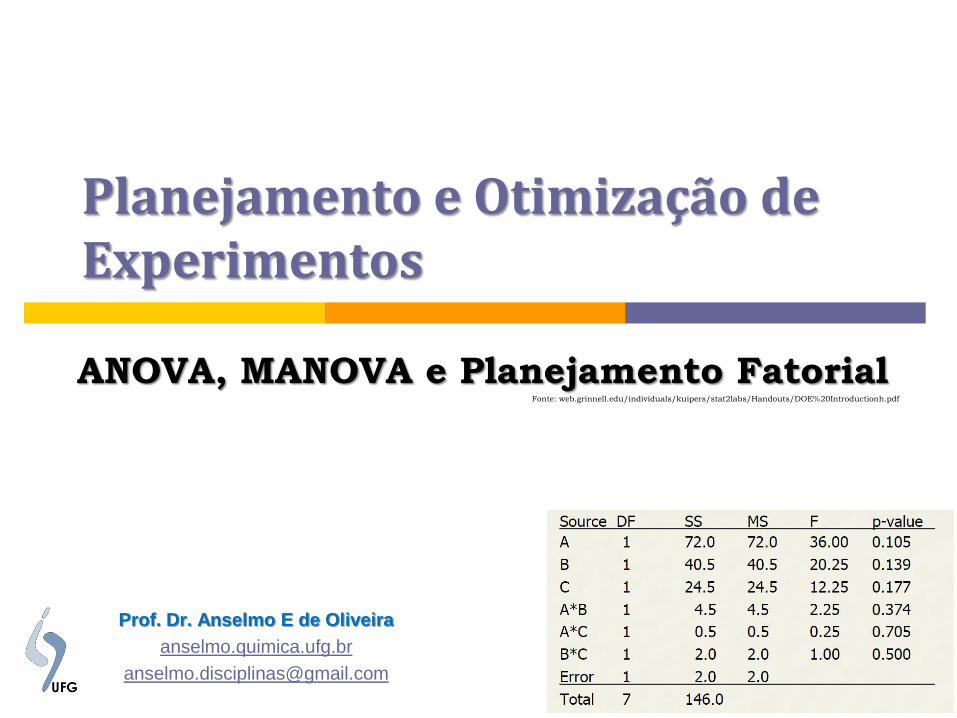
ANOVA, MANOVA e Planejamento Fatorial Fonte: web.grinnell.edu/individuals/kuipers/stat2labs/Handouts/DOE%20Introductionh.pdf
Prof. Dr. Anselmo E de Oliveira
anselmo.quimica.ufg.br
[email protected]
Page 2
ANOVA and Factorial Design
ANOVA is a statistical technique used to
investigate and model the relationship between a
response variable and one or more independent
variables
Each explanatory variable (factor) consists of two
or more categories (levels)
ANOVA tests the null hypothesis that the
population means of each level are equal, versus
the alternative hypothesis that at least one of the
level means are not all equal.
Page 3
ANOVA and Factorial Design
Example 1: a 2003 study was conducted to test if
there was a difference in attitudes towards science
between boys and girls
Factor: gender with Levels: boys and girls
Unit (Experimental Unit or Subject): each individual child
Response Variable: Each child’s score on an attitude
assessment
Null Hypothesis: boys and girls have the same mean
score on the assessment
Alternative Hypothesis: boys and girls have different
mean scores on the assessment.
Page 4
ANOVA and Factorial Design
Example 1 can be analyzed with ANOVA or a two-
sample t-test
In both methods the experimenter collects sample
data and calculates averages. If the means of the
two levels are “significantly” far apart, the
experimenter will accept the alternative hypothesis.
While their calculations differ, ANOVA and two-
sample t-tests always give identical results in
hypothesis tests for means with one factor and
two levels.
Page 5
ANOVA and Factorial Design
Unfortunately, modeling real world phenomena
often requires more than just one factor. In order
to understand the sources of variability in a
phenomenon of interest, ANOVA can
simultaneously test several factors each with
several levels
Although there are situations where t-tests should
be used to simultaneously test the means of
multiple levels, doing so create a multiple
comparison problem
Page 6
ANOVA and Factorial Design
Key steps in designing an experiment include:
Identify factors of interest and a response variable
Determine appropriate levels for each explanatory
variable
Determine a design structure
Randomize the order in which each set of conditions is
run and collect the data
Organize the results in order to draw appropriate
conclusions
Page 7
Multivariate ANOVA (MANOVA)
Example 2: Soft drink modeling problem
A soft drink bottler is interested in obtaining
more uniform fill heights in the bottles produced by
his manufacturing process. The filling machine
theoretically fills each bottle to the correct target
height, but in practice, there is variation around
this target, and the bottler would like to
understand better the sources of this variability
and eventually reduce it. The engineer can control
three variables during the filling process (each at
two levels).
(Montgomery p. 208)
Page 8
Multivariate ANOVA (MANOVA)
Factor A: Carbonation with levels: 10% and 12%
Factor B: Operating pressure in the filler with
levels: 25 and 30 psi
Factor C: Line speed with levels: 200 and 250
bottles produced per minute (bpm)
Unit: Each bottle response variable: deviation
from the target fill height
Six hypotheses will be simultaneously tested.
Page 9
Multivariate ANOVA (MANOVA)
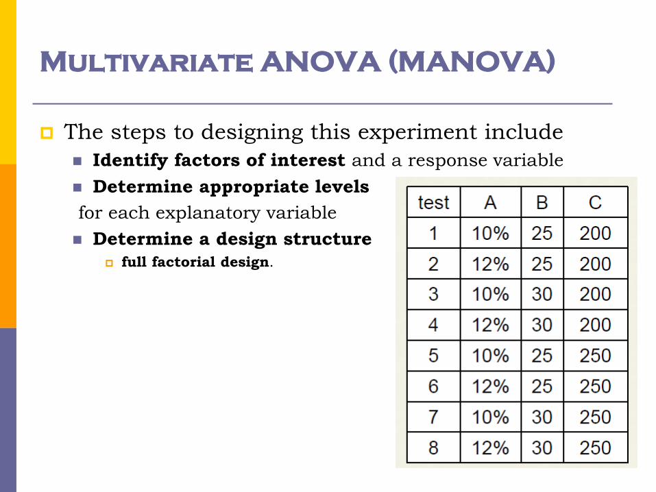
The steps to designing this experiment include
Identify factors of interest and a response variable
Determine appropriate levels
for each explanatory variable
Determine a design structure
full factorial design.
Page 10
Multivariate ANOVA (MANOVA)
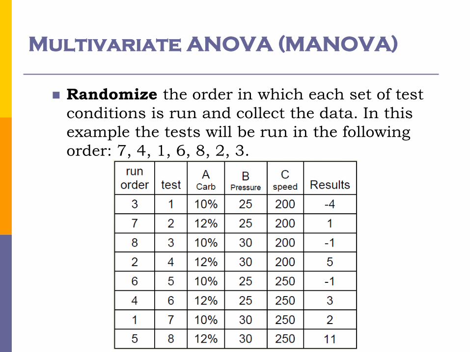
Randomize the order in which each set of test
conditions is run and collect the data. In this
example the tests will be run in the following
order: 7, 4, 1, 6, 8, 2, 3.
Page 11
Main Effects
Often the impact of changing factor levels are described as effect
sizes. A main effect is the difference between the factor average
and the grand mean
Effect of A+ = average of factor A+ minus the grand mean
= 5 – 2 = 3
Effect of C- = 0.25 – 2 = -1.75
Effect sizes determine which factors have the most significant
impact on the results. Calculations in ANOVA determine the
significance of each factor based on these effect calculations
subtract the
grand mean
(2) from each
cell
Page 12
Main Effects
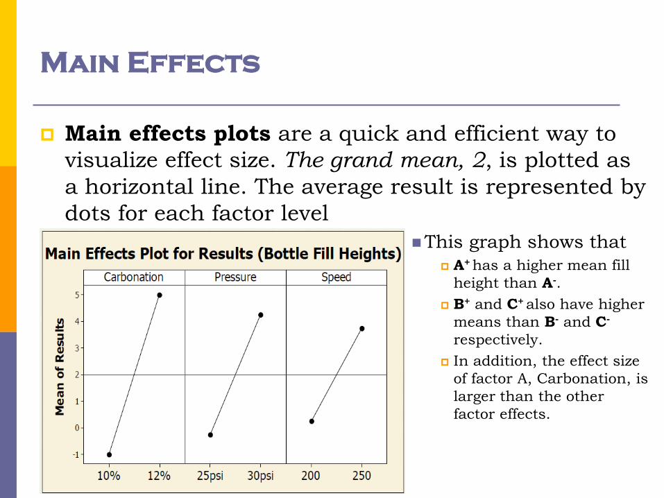
Main effects plots are a quick and efficient way to
visualize effect size. The grand mean, 2, is plotted as
a horizontal line. The average result is represented by
dots for each factor level
This graph shows that
A+ has a higher mean fill
height than A-.
B+ and C+ also have higher
means than B- and C-
respectively.
In addition, the effect size
of factor A, Carbonation, is
larger than the other
factor effects.
Page 13
Interaction Effects
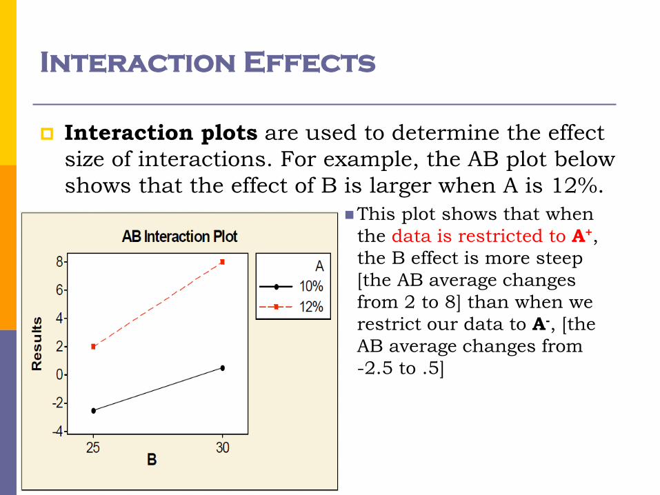
Interaction plots are used to determine the effect
size of interactions. For example, the AB plot below
shows that the effect of B is larger when A is 12%.
This plot shows that when
the data is restricted to A+,
the B effect is more steep
[the AB average changes
from 2 to 8] than when we
restrict our data to A-, [the
AB average changes from
-2.5 to .5]
Page 14
Interaction Effects
The following plot shows the interaction (or 2-way effects) of all three
factors. When the lines are parallel, interaction effects are 0. The
more different the slopes, the more influence the interaction effect has
on the results. To visualize these effects, the Y axis is always the
same for each combination of factors. This graph shows that the AB
interaction effect is the largest
This plot shows that the B-C-
average (i.e. B set to 25 and C
set to 200) is -1.5.The B-C+
average is 1
Page 15
Mathematical Calculations
Effect plots help visualize the impact of each factor
combination and identify which factors are most
influential. However, a statistical hypotheses test is
needed in order to determine if any of these effects
are significant
Analysis of variance (ANOVA) consists of simultaneous
hypothesis tests to determine if any of the effects are
significant
Note that saying “factor effects are zero” is equivalent to
saying “the means for all levels of a factor are equal”. Thus,
for each factor combination ANOVA tests the null
hypothesis that the population means of each level are
equal, versus them not all being equal.
Page 16
Mathematical Calculations
Several calculations will be made for each main
factor and interaction term
Sum of Squares (SS): sum of all the squared effects for
each factor
Degrees of Freedom (df): number of free units of
information
Mean Square (MS) = SS/df for each factor
Mean Square Error (MSE): pooled variance of samples
within each level
F-statistic = MS for each factor/MSE
Page 17
Mathematical Calculations
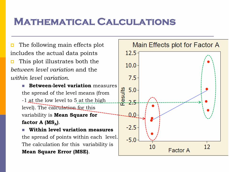
The following main effects plot
includes the actual data points
This plot illustrates both the
between level variation and the
within level variation.
Between-level variation measures
the spread of the level means (from
-1 at the low level to 5 at the high
level). The calculation for this
variability is Mean Square for
factor A (MSA).
Within level variation measures
the spread of points within each level.
The calculation for this variability is
Mean Square Error (MSE).
Page 18
Mathematical Calculations
To determine if the difference between level means
of factor A is significant, we compare the between-
level variation of A (MSA) to the within-level
variation (MSE)
If the MSA is much larger than MSE, it is reasonable to
conclude that their truly is a difference between level
means and the difference we observed in our sample runs
was not simply due to random chance.
Page 19
Mathematical Calculations
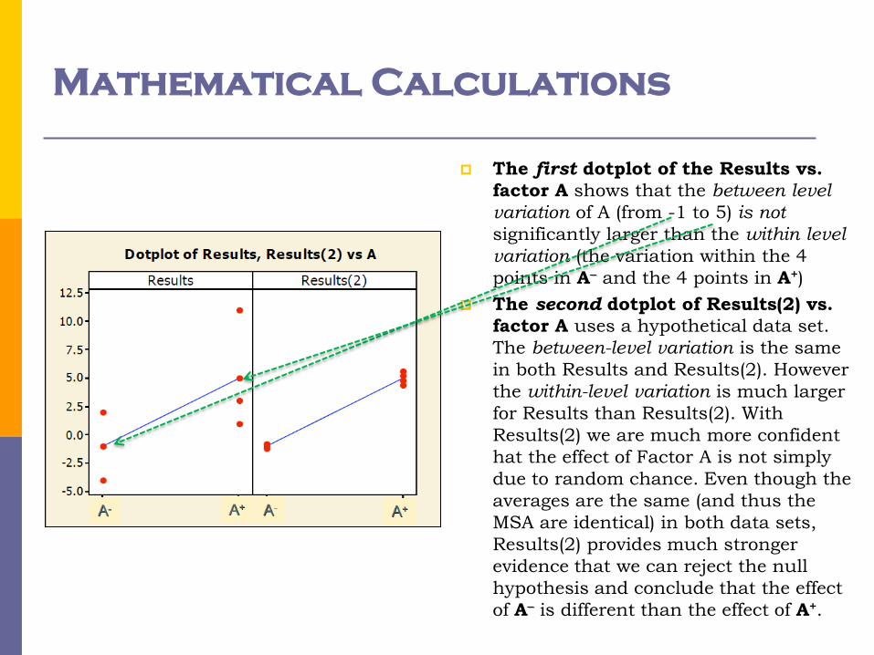
The first dotplot of the Results vs.
factor A shows that the between level
variation of A (from -1 to 5) is not
significantly larger than the within level
variation (the variation within the 4
points in A- and the 4 points in A+)
The second dotplot of Results(2) vs.
factor A uses a hypothetical data set.
The between-level variation is the same
in both Results and Results(2). However
the within-level variation is much larger
for Results than Results(2). With
Results(2) we are much more confident
hat the effect of Factor A is not simply
due to random chance. Even though the
averages are the same (and thus the
MSA are identical) in both data sets,
Results(2) provides much stronger
evidence that we can reject the null
hypothesis and conclude that the effect
of A- is different than the effect of A+.
Page 20
Mathematical Calculations
Sum of Squares (SS) is calculated by summing the
squared factor effect for each run
Page 21
Mathematical Calculations
In the previous table, the effect of A- = −3 and
effect of A+ = 3 were calculated by subtracting the
grand mean from the level averages.
The formula for calculating effects A- is 𝑦 1 − 𝑦 and A+ is
𝑦 2 − 𝑦
𝑦 1 is the factor A average for level 𝑖
In our example, 𝑖 = 1 represents A- and 𝑦 1 = −1 also 𝑦 2 = 5
𝑦 is the grand mean
In our example, 𝑦 = 2
To calculate SSA, the effect is squared for each run
and then summed. Note that there are 𝑛1 = 4 runs
for A- and 𝑛2 = 4 runs for A+
4 𝑦 1 − 𝑦 2 + 4 𝑦 2 − 𝑦
2 = 72
Page 22
Mathematical Calculations
The generalized formula for SSA is
𝑆𝑆𝐴 = 𝑛𝑖 𝑦 𝑖 − 𝑦 2
𝐼
𝑖=1
𝐼 is the number of levels in factor A, in our example, 𝐼 = 2
𝑛𝑖 is the number of samples in the 𝑖th level of factor A,
𝑛1 = 4 and 𝑛2 = 4
𝑦 𝑖 is the factor A average for level 𝑖 and 𝑦 is the grand
mean
In the same manner, SSB and SSC are calculated
by
𝑆𝑆𝐵 = 𝑛𝑗 𝑦 𝑗 − 𝑦 2
𝐽
𝑗=1
𝑆𝑆𝐶 = 𝑛𝑘 𝑦 𝑘 − 𝑦 2
𝐾
𝑘=1
Page 23
Mathematical Calculations
Sum of Squares (SS) for interactions is also
calculated by summing the squared factor effect for
each run
𝑆𝑆𝐴𝐵 = 𝑛𝑖𝑗 𝑦 𝑖𝑗 − 𝑦 𝑖 − 𝑦 𝑗 − 𝑦 2
𝐼
𝑖=1
𝐽
𝑗=1
𝑦 − 𝑦 1 = 2 − 1.25 =
𝑦 − 𝑦 2 = 2 − 2.75 =
...
Page 24
Mathematical Calculations
Degrees of Freedom (df)= number of free units of
information
In the example provided, there are 2 levels of factor A.
Since we require that the effects sum to 0, knowing A-
automatically forces a known A+. If there are 𝐼 levels for
factor A, one level is fixed if we know the other 𝐼 − 1 levels.
Thus, when there are 𝐼 levels for a main factor of interest,
there is 𝐼 − 1 free pieces of information
𝑑𝑓𝐴 = 𝐼 − 1
𝑑𝑓𝐵 = 𝐽 − 1
𝑑𝑓𝐶 = 𝐾 − 1
Page 25
Mathematical Calculations
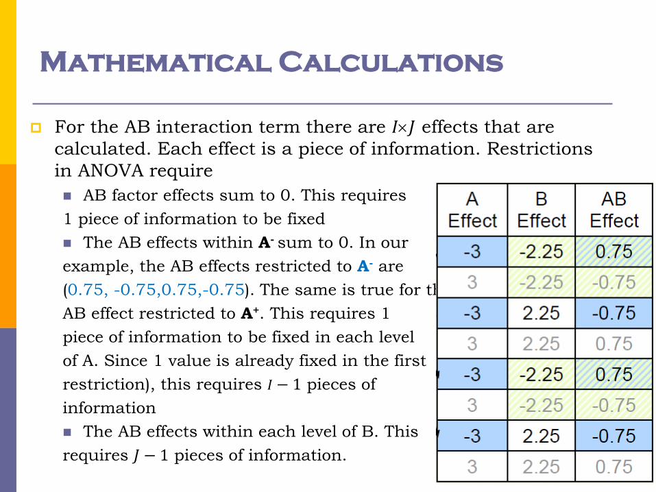
For the AB interaction term there are 𝐼𝐽 effects that are
calculated. Each effect is a piece of information. Restrictions
in ANOVA require
AB factor effects sum to 0. This requires
1 piece of information to be fixed
The AB effects within A- sum to 0. In our
example, the AB effects restricted to A- are
(0.75, -0.75,0.75,-0.75). The same is true for the
AB effect restricted to A+. This requires 1
piece of information to be fixed in each level
of A. Since 1 value is already fixed in the first
restriction), this requires 𝐼 − 1 pieces of
information
The AB effects within each level of B. This
requires 𝐽 − 1 pieces of information.
Page 26
Mathematical Calculations
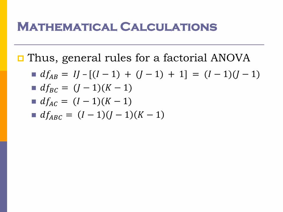
Thus, general rules for a factorial ANOVA
𝑑𝑓𝐴𝐵 = 𝐼𝐽 – [(𝐼 − 1) + (𝐽 − 1) + 1] = (𝐼 − 1)(𝐽 − 1)
𝑑𝑓𝐵𝐶 = (𝐽 − 1)(𝐾 − 1)
𝑑𝑓𝐴𝐶 = (𝐼 − 1)(𝐾 − 1)
𝑑𝑓𝐴𝐵𝐶 = 𝐼 − 1 𝐽 − 1 𝐾 − 1
Page 27
Mathematical Calculations
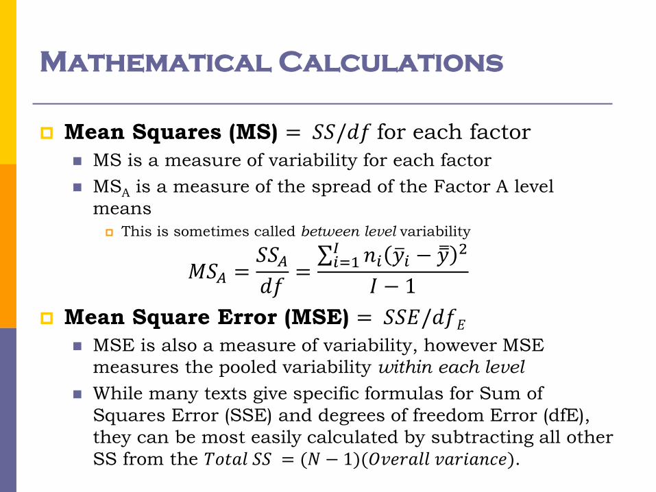
Mean Squares (MS) = 𝑆𝑆/𝑑𝑓 for each factor
MS is a measure of variability for each factor
MSA is a measure of the spread of the Factor A level
means
This is sometimes called between level variability
𝑀𝑆𝐴 =𝑆𝑆𝐴𝑑𝑓= 𝑛𝑖 𝑦 𝑖 − 𝑦
2𝐼𝑖=1
𝐼 − 1
Mean Square Error (MSE) = 𝑆𝑆𝐸/𝑑𝑓𝐸 MSE is also a measure of variability, however MSE
measures the pooled variability within each level
While many texts give specific formulas for Sum of
Squares Error (SSE) and degrees of freedom Error (dfE),
they can be most easily calculated by subtracting all other
SS from the 𝑇𝑜𝑡𝑎𝑙 𝑆𝑆 = (𝑁 − 1)(𝑂𝑣𝑒𝑟𝑎𝑙𝑙 𝑣𝑎𝑟𝑖𝑎𝑛𝑐𝑒).
Page 28
Mathematical Calculations
F-statistic = MS for each factor/MSE
The F-statistic is a ratio of the between variability over the within
variability
If the true population mean of A- equals true population mean of A+,
then we would expect the variation between levels in our sample runs to
be equivalent to the variation within levels. Thus we would expect the F-
statistic would be close to 1
If the F-statistic is large, it seems unlikely that the population means of
each level of factor A are truly equal
Mathematical theory proves that if the appropriate assumptions hold,
the F-statistic follows an F distribution with 𝑑𝑓𝐴 (if testing factor A) and
𝑑𝑓𝐸 degrees of freedom
The P-value is looked up in an F table and gives the likelihood of
observing an F statistic at least this extreme (at least this large)
assuming that the true population factor has equal level means. Thus,
when the P-value is small (i.e. less than 0.05 or 0.1) the effect size of that
factor is statistically significant. Ex: http://www.stat.tamu.edu/~west/applets/fdemo.html
Page 29
Mathematical Calculations
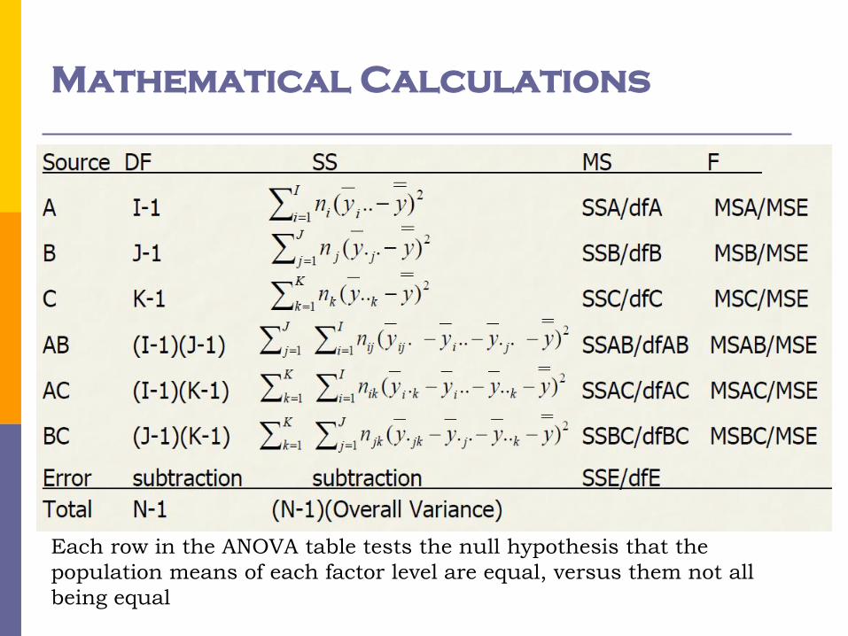
Each row in the ANOVA table tests the null hypothesis that the
population means of each factor level are equal, versus them not all
being equal
Page 30
Mathematical Calculations
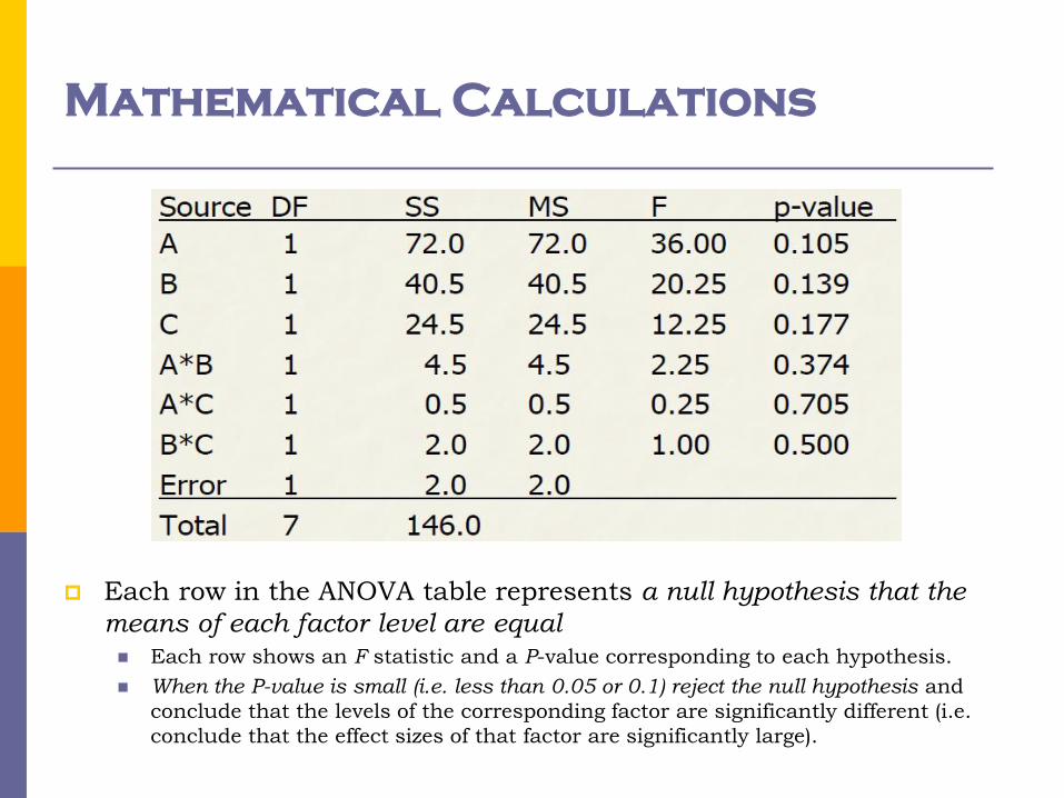
Each row in the ANOVA table represents a null hypothesis that the
means of each factor level are equal Each row shows an F statistic and a P-value corresponding to each hypothesis.
When the P-value is small (i.e. less than 0.05 or 0.1) reject the null hypothesis and
conclude that the levels of the corresponding factor are significantly different (i.e.
conclude that the effect sizes of that factor are significantly large).
Page 31
Mathematical Calculations
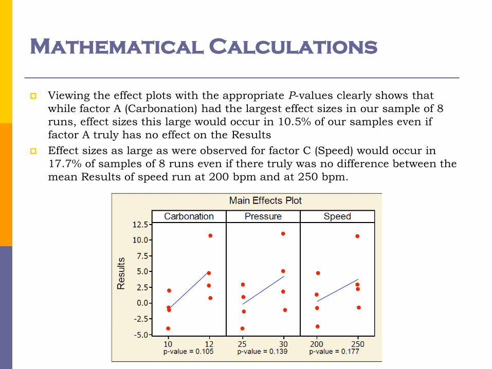
Viewing the effect plots with the appropriate P-values clearly shows that
while factor A (Carbonation) had the largest effect sizes in our sample of 8
runs, effect sizes this large would occur in 10.5% of our samples even if
factor A truly has no effect on the Results
Effect sizes as large as were observed for factor C (Speed) would occur in
17.7% of samples of 8 runs even if there truly was no difference between the
mean Results of speed run at 200 bpm and at 250 bpm.
Page 32
Mathematical Calculations
The BC interaction plot with the appropriate P-value shows that the lack of
parallelism between the lines is relatively small based on the sampling
variability. The p-value also shows that we would expect a lack of parallelism
at least this large in 50% of our samples even if no interaction existed
between factor B (pressure) and factor C (speed)
Page 33
Mathematical Calculations
Consider a variation of the bottle filling experiment. Suppose that only two
levels are used so that the experiment is a 23 factorial design with two
replicates.
ANOVA
Model equation
Model surface
ANOVA for regression
run
A
Carb
B
Pressure
C
Speed Result1 Result2
1 10 25 200 -3 -1
2 12 25 200 0 1
3 10 30 200 -1 0
4 12 30 200 2 3
5 10 25 250 -1 0
6 12 25 250 2 1
7 10 30 250 1 1
8 12 30 250 6 5
Page 34
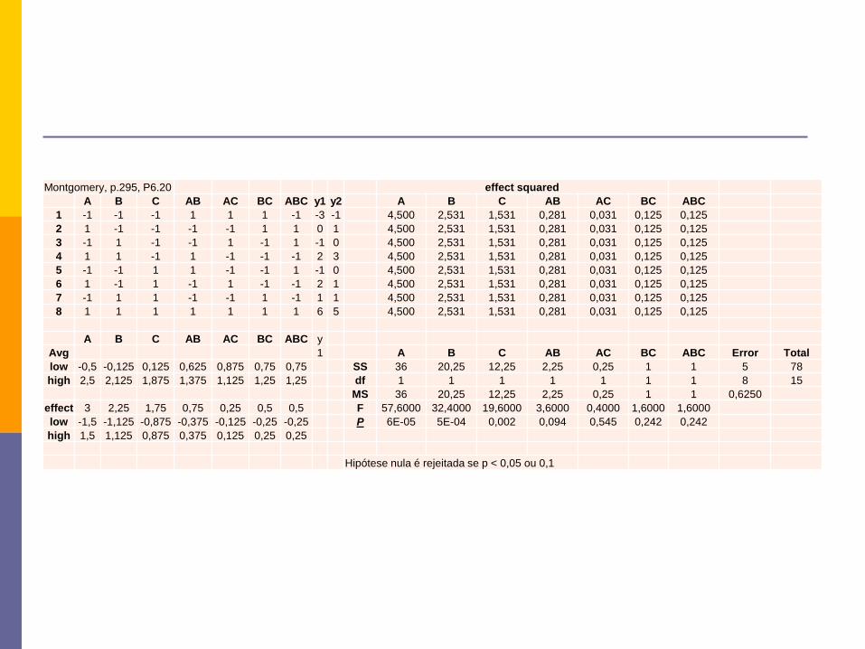
Montgomery, p.295, P6.20 effect squared
A B C AB AC BC ABC y1 y2 A B C AB AC BC ABC
1 -1 -1 -1 1 1 1 -1 -3 -1 4,500 2,531 1,531 0,281 0,031 0,125 0,125
2 1 -1 -1 -1 -1 1 1 0 1 4,500 2,531 1,531 0,281 0,031 0,125 0,125
3 -1 1 -1 -1 1 -1 1 -1 0 4,500 2,531 1,531 0,281 0,031 0,125 0,125
4 1 1 -1 1 -1 -1 -1 2 3 4,500 2,531 1,531 0,281 0,031 0,125 0,125
5 -1 -1 1 1 -1 -1 1 -1 0 4,500 2,531 1,531 0,281 0,031 0,125 0,125
6 1 -1 1 -1 1 -1 -1 2 1 4,500 2,531 1,531 0,281 0,031 0,125 0,125
7 -1 1 1 -1 -1 1 -1 1 1 4,500 2,531 1,531 0,281 0,031 0,125 0,125
8 1 1 1 1 1 1 1 6 5 4,500 2,531 1,531 0,281 0,031 0,125 0,125
A B C AB AC BC ABC y
Avg 1 A B C AB AC BC ABC Error Total
low -0,5 -0,125 0,125 0,625 0,875 0,75 0,75 SS 36 20,25 12,25 2,25 0,25 1 1 5 78
high 2,5 2,125 1,875 1,375 1,125 1,25 1,25 df 1 1 1 1 1 1 1 8 15
MS 36 20,25 12,25 2,25 0,25 1 1 0,6250
effect 3 2,25 1,75 0,75 0,25 0,5 0,5 F 57,6000 32,4000 19,6000 3,6000 0,4000 1,6000 1,6000
low -1,5 -1,125 -0,875 -0,375 -0,125 -0,25 -0,25 P 6E-05 5E-04 0,002 0,094 0,545 0,242 0,242
high 1,5 1,125 0,875 0,375 0,125 0,25 0,25
Hipótese nula é rejeitada se p < 0,05 ou 0,1