arXiv:1205.5060v2 [astro-ph.EP] 11 Mar 2013 Astronomy & Astrophysics manuscript no. wasp33˙v9˙aph c ESO 2018 May 23, 2018 Comprehensive time series analysis of the transiting extrasolar planet WASP-33b G. Kov´ acs 1,2 , T. Kov´ acs 1 , J. D. Hartman 3 , G. ´ A. Bakos 3,5 , A. Bieryla 4 , D. Latham 4 , R. W. Noyes 4 , Zs. Reg´ aly 1 , G. A. Esquerdo 4 1 Konkoly Observatory, Budapest, Hungary e-mail: [email protected]2 Department of Physics and Astrophysics, University of North Dakota, Grand Forks, ND, USA 3 Department of Astrophysical Sciences, Princeton University, Princeton, NJ, USA 4 Harvard-Smithsonian Center for Astrophysics, Cambridge, MA, USA 5 Alfred P. Sloan Research Fellow May 22, 2012; March 5, 2013 ABSTRACT Context. HD 15082 (WASP-33) is the hottest and fastest rotating star known to harbor a transiting extrasolar planet (WASP-33b). The lack of high precision radial velocity (RV) data stresses the need for precise light curve analysis and gathering further RV data. Aims. By using available photometric and RV data, we perform a blend analysis, compute more accurate system parameters, confine the planetary mass and attempt to cast light on the observed transit anomalies. Methods. We combine the original HATNet observations and various followup data to jointly analyze the signal content and extract the transit component and use our RV data to aid the global parameter determination. Results. The blend analysis of the combination of multicolor light curves yields the first independent confirmation of the planetary nature of WASP-33b. We clearly identify three frequency components in the 15–21 d −1 regime with amplitudes 7–5 mmag. These frequencies correspond to the δ Scuti-type pulsation of the host star. None of these pulsation frequencies or their low-order linear combinations are in close resonance with the orbital frequency. We show that these pulsation components explain some but not all of the observed transit anomalies. The grand-averaged transit light curve shows that there is a ∼ 1.5 mmag brightening shortly after the planet passes the mid-transit phase. Although the duration and amplitude of this brightening varies, it is visible even through the direct inspections of the individual transit events (some 40–60% of the followup light curves show this phenomenon). We suggest that the most likely explanation of this feature is the presence of a well-populated spot belt which is highly inclined to the orbital plane. This geometry is consistent with the inference from the spectroscopic anomalies. Finally, we constrain the planetary mass to M p = 3.27 ± 0.73 M J by using our RV data collected by the TRES spectrograph. Key words. stars: variables: δ Sct – methods: data analysis – planetary systems – stars: individual: WASP-33 1. Introduction The short-period (P = 1.22 d) transiting extrasolar planet WASP-33b was discovered by Christian et al. (2006) in the course of the transit survey conducted by the WASP project (Pollacco et al. 2006). The host star, HD 15082, is a bright, V = 8.3 mag A-type star with a high projected rotational ve- locity of ∼ 90 km s −1 . As a result, high precision radial veloc- ity (RV) measurements usually demanded by the planet verifi- cation and planet mass estimation processes are very difficult to take. Followup spectroscopic observations by Collier Cameron et al. (2010, hereafter CC10) could only yield an upper limit of 4.1M J on the planetary mass but no bisector analysis could be performed due to the several km s −1 scatter of the measured RV values. However, due to the large rotational velocity, the authors were able to utilize the surface velocity field mapping capability of the orbiting planet and showed very clearly that the orbital revolution was highly inclined (i.e., retrograde) in respect to the stellar rotational axis. The WASP-33 system stands out from the other transiting systems not only for its highest rotation rate and highest T eff of 7400 K (CC10) but also because of the planet’s highest substellar temperature (T 0 = 3800 K, see Sect. 9). Due to the high incident flux and the early spectral type of the star we expect that a large amount of UV radiation is deposited in the planet’s atmosphere. This, together with its high Roche-lobe filling factor (see Budaj 2011) make this system perhaps the best candidate for studying effective planetary envelope evaporation and mass flow onto the host star. Due to its brightness and significant transit depth of ∼ 14 mmag, the WASP-33 system is highly suitable for followup photometric observations. Some 80 1 events have been observed over the years by professional and amateur astronomers. Most of these light curves (LCs) display various anomalies, such as tran- sit depth variation, mid-transit humps, tilted full transit phase, asymmetric ingress/egress phases and small-amplitude oscilla- tions. Although not all of these variations are necessarily real, it is clear that the system is peculiar and very much worth for further attention. WASP-33 was also observed by HATNet (Bakos et al., 2002, 2004) in the course of the search for transiting extra- solar planets (TEPs). After assigning the ‘candidate’ status to the target in January 2010, a followup reconnaissance spec- troscopy conducted by the TRES spectrograph (F˝ ur´ esz 2008) 1 http://var2.astro.cz/ETD/ 1
2 Department of Physics and Astrophysics, University of North Dakota, Grand Forks, ND, USA3 Department of Astrophysical Sciences, Princeton University, Princeton, NJ, USA4 Harvard-Smithsonian Center for Astrophysics, Cambridge,MA, USA5 Alfred P. Sloan Research Fellow
May 22, 2012; March 5, 2013
ABSTRACT
Context. HD 15082 (WASP-33) is the hottest and fastest rotating star known to harbor a transiting extrasolar planet (WASP-33b). Thelack of high precision radial velocity (RV) data stresses the need for precise light curve analysis and gathering further RV data.Aims. By using available photometric and RV data, we perform a blend analysis, compute more accurate system parameters, confinethe planetary mass and attempt to cast light on the observed transit anomalies.Methods. We combine the original HATNet observations and various followup data to jointly analyze the signal content and extractthe transit component and use our RV data to aid the global parameter determination.Results. The blend analysis of the combination of multicolor light curves yields the first independent confirmation of the planetarynature of WASP-33b. We clearly identify three frequency components in the 15–21d−1 regime with amplitudes 7–5 mmag. Thesefrequencies correspond to theδ Scuti-type pulsation of the host star. None of these pulsation frequencies or their low-order linearcombinations are in close resonance with the orbital frequency. We show that these pulsation components explain some but not allof the observed transit anomalies. The grand-averaged transit light curve shows that there is a∼ 1.5 mmag brightening shortly afterthe planet passes the mid-transit phase. Although the duration and amplitude of this brightening varies, it is visible even through thedirect inspections of the individual transit events (some 40–60% of the followup light curves show this phenomenon). Wesuggestthat the most likely explanation of this feature is the presence of a well-populated spot belt which is highly inclined tothe orbitalplane. This geometry is consistent with the inference from the spectroscopic anomalies. Finally, we constrain the planetary mass toMp = 3.27± 0.73 MJ by using our RV data collected by the TRES spectrograph.
Key words. stars: variables:δ Sct – methods: data analysis – planetary systems – stars: individual: WASP-33
1. Introduction
The short-period (P = 1.22 d) transiting extrasolar planetWASP-33b was discovered by Christian et al. (2006) in thecourse of the transit survey conducted by the WASP project(Pollacco et al. 2006). The host star, HD 15082, is a bright,V = 8.3 mag A-type star with a high projected rotational ve-locity of ∼ 90 km s−1. As a result, high precision radial veloc-ity (RV) measurements usually demanded by the planet verifi-cation and planet mass estimation processes are very difficult totake. Followup spectroscopic observations by Collier Cameronet al. (2010, hereafter CC10) could only yield an upper limitof4.1 MJ on the planetary mass but no bisector analysis could beperformed due to the several km s−1 scatter of the measured RVvalues. However, due to the large rotational velocity, the authorswere able to utilize the surface velocity field mapping capabilityof the orbiting planet and showed very clearly that the orbitalrevolution was highly inclined (i.e., retrograde) in respect to thestellar rotational axis.
The WASP-33 system stands out from the other transitingsystems not only for its highest rotation rate and highestTeff of7400 K (CC10) but also because of the planet’s highest substellartemperature (T0 = 3800 K, see Sect. 9). Due to the high incident
flux and the early spectral type of the star we expect that a largeamount of UV radiation is deposited in the planet’s atmosphere.This, together with its high Roche-lobe filling factor (see Budaj2011) make this system perhaps the best candidate for studyingeffective planetary envelope evaporation and mass flow onto thehost star.
Due to its brightness and significant transit depth of∼14 mmag, the WASP-33 system is highly suitable for followupphotometric observations. Some 801 events have been observedover the years by professional and amateur astronomers. Most ofthese light curves (LCs) display various anomalies, such astran-sit depth variation, mid-transit humps, tilted full transit phase,asymmetric ingress/egress phases and small-amplitude oscilla-tions. Although not all of these variations are necessarilyreal,it is clear that the system is peculiar and very much worth forfurther attention.
WASP-33 was also observed by HATNet (Bakos et al.,2002, 2004) in the course of the search for transiting extra-solar planets (TEPs). After assigning the ‘candidate’ status tothe target in January 2010, a followup reconnaissance spec-troscopy conducted by the TRES spectrograph (Furesz 2008)
has led to the conclusion that the rotational velocity was veryhigh. Nevertheless, we continued the spectroscopic followup andfound that the low velocity amplitude may suggest the presenceof a planetary companion. After the SuperWASP announcementwe stopped pursuing this target but here we utilize both the RVand the photometric (HATNet and our early followup) data.
In this paper we perform a comprehensive time series anal-ysis by utilizing the HATNet data, the followup LCs depositedat the Exoplanet Transit Database (ETD, see Poddany, Brat, &Pejcha (2010)), other published photometric data and new LCsfrom the Fred Lawrence Whipple and Konkoly observatories.2
Our goal is to verify the planetary nature of WASP-33b purelyfrom photometry (the ‘Kepler-way’ of system validation – see,e.g., Muirhead et al. 2012), to derive more accurate system pa-rameters and examine the possible causes of light curve anoma-lies. We also use our RV archive, based on the observations ob-tained by the TRES spectrograph, to improve the mass estimateof the planet.
2. HATNet detection
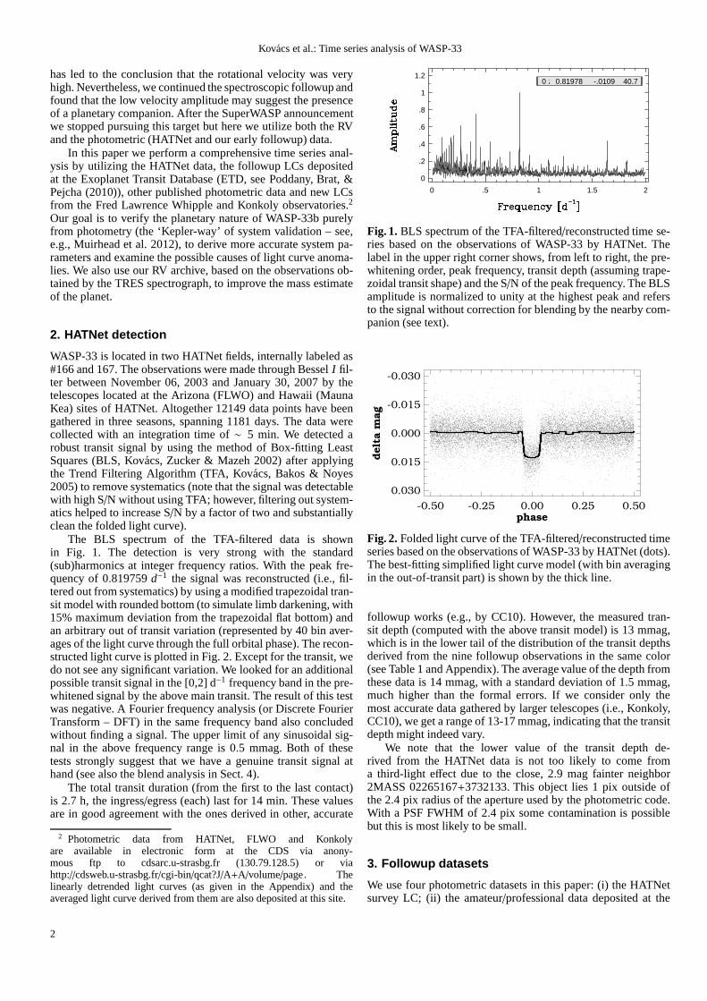
WASP-33 is located in two HATNet fields, internally labeled as#166 and 167. The observations were made through BesselI fil-ter between November 06, 2003 and January 30, 2007 by thetelescopes located at the Arizona (FLWO) and Hawaii (MaunaKea) sites of HATNet. Altogether 12149 data points have beengathered in three seasons, spanning 1181 days. The data werecollected with an integration time of∼ 5 min. We detected arobust transit signal by using the method of Box-fitting LeastSquares (BLS, Kovacs, Zucker & Mazeh 2002) after applyingthe Trend Filtering Algorithm (TFA, Kovacs, Bakos & Noyes2005) to remove systematics (note that the signal was detectablewith high S/N without using TFA; however, filtering out system-atics helped to increase S/N by a factor of two and substantiallyclean the folded light curve).
The BLS spectrum of the TFA-filtered data is shownin Fig. 1. The detection is very strong with the standard(sub)harmonics at integer frequency ratios. With the peak fre-quency of 0.819759d−1 the signal was reconstructed (i.e., fil-tered out from systematics) by using a modified trapezoidal tran-sit model with rounded bottom (to simulate limb darkening, with15% maximum deviation from the trapezoidal flat bottom) andan arbitrary out of transit variation (represented by 40 binaver-ages of the light curve through the full orbital phase). The recon-structed light curve is plotted in Fig. 2. Except for the transit, wedo not see any significant variation. We looked for an additionalpossible transit signal in the [0,2] d−1 frequency band in the pre-whitened signal by the above main transit. The result of thistestwas negative. A Fourier frequency analysis (or Discrete FourierTransform – DFT) in the same frequency band also concludedwithout finding a signal. The upper limit of any sinusoidal sig-nal in the above frequency range is 0.5 mmag. Both of thesetests strongly suggest that we have a genuine transit signalathand (see also the blend analysis in Sect. 4).
The total transit duration (from the first to the last contact)is 2.7 h, the ingress/egress (each) last for 14 min. These valuesare in good agreement with the ones derived in other, accurate
2 Photometric data from HATNet, FLWO and Konkolyare available in electronic form at the CDS via anony-mous ftp to cdsarc.u-strasbg.fr (130.79.128.5) or viahttp://cdsweb.u-strasbg.fr/cgi-bin/qcat?J/A+A/volume/page. Thelinearly detrended light curves (as given in the Appendix) and theaveraged light curve derived from them are also deposited atthis site.
0 .5 1 1.5 2
0
.2
.4
.6
.8
1
1.2
0 0.81978 -.0109 40.7
Fig. 1. BLS spectrum of the TFA-filtered/reconstructed time se-ries based on the observations of WASP-33 by HATNet. Thelabel in the upper right corner shows, from left to right, thepre-whitening order, peak frequency, transit depth (assuming trape-zoidal transit shape) and the S/N of the peak frequency. The BLSamplitude is normalized to unity at the highest peak and refersto the signal without correction for blending by the nearby com-panion (see text).
-0.50 -0.25 0.00 0.25 0.50
phase
0.030
0.015
0.000
-0.015
-0.030delt
a m
ag
Fig. 2. Folded light curve of the TFA-filtered/reconstructed timeseries based on the observations of WASP-33 by HATNet (dots).The best-fitting simplified light curve model (with bin averagingin the out-of-transit part) is shown by the thick line.
followup works (e.g., by CC10). However, the measured tran-sit depth (computed with the above transit model) is 13 mmag,which is in the lower tail of the distribution of the transit depthsderived from the nine followup observations in the same color(see Table 1 and Appendix). The average value of the depth fromthese data is 14 mmag, with a standard deviation of 1.5 mmag,much higher than the formal errors. If we consider only themost accurate data gathered by larger telescopes (i.e., Konkoly,CC10), we get a range of 13-17 mmag, indicating that the transitdepth might indeed vary.
We note that the lower value of the transit depth de-rived from the HATNet data is not too likely to come froma third-light effect due to the close, 2.9 mag fainter neighbor2MASS 02265167+3732133. This object lies 1 pix outside ofthe 2.4 pix radius of the aperture used by the photometric code.With a PSF FWHM of 2.4 pix some contamination is possiblebut this is most likely to be small.
3. Followup datasets
We use four photometric datasets in this paper: (i) the HATNetsurvey LC; (ii) the amateur/professional data deposited at the
LC# Date [UT] N FIL Source LC# Date [UT] N FIL Source
01 2003 – 2007 2285 I HATNet 23X 2011-10-13 505 J Kitt Peak02X 2010-03-03 275 z FLWO 24 2011-10-23 96 C LTremosa03 2010-08-23 245 R KHose 25 2011-11-12 291 I Konkoly04 2010-08-26 282 R FHormuth 26 2011-11-12 79 V GCorfini05 2010-08-26 163 R RNaves 27 2011-11-14 907 V SDvorak06 2010-09-17 220 R TScarmato 28X 2011-11-23 404 R JGaitan07 2010-09-28 277 R EHerrero 29X 2011-11-23 127 R RNaves08X 2010-10-11 598 B WDauberman 30 2011-11-24 446 I Konkoly09X 2010-10-15 191 R RNaves 31X 2011-11-24 177 V RNaves10 2010-10-20 434 R CLopresti 32 2011-12-01 888 I TDax11 2010-10-20 138 R RNaves 33 2011-12-10 146 C FGarcia12 2010-11-03 451 z’ Kitt Peak 34 2011-12-15 109 I JGaitan13 2010-11-19 863 V SDvorak 35X 2011-12-20 149 V DGorshanov14 2010-12-06 1254 C SShadick 36 2011-12-21 134 V RNaves15 2010-12-25 440 C AMaurice 37 2011-12-27 230 C JLopesino16 2011-01-05 437 C CWiedemair 38X 2012-01-01 113 V RNaves17 2011-01-13 778 V SDvorak 39X 2012-01-01 420 C JLopesino18 2011-01-16 238 C SGajdos 40 2012-01-09 316 I SShadick19 2011-09-21 311 I SShadick 41 2012-01-12 130 V RNaves20 2011-09-24 468 C LBrat 42 2012-01-20 534 I SShadick21X 2011-10-05 196 R RNaves 43 2012-02-11 365 I SShadick22 2011-10-13 310 Hα Kitt Peak
Comments:Header:LC#: light curve identification number used in this paper; Date: starting date of the observations; N: number of data points (may differfrom those given at the ETD site, e.g., because of multiple items); FIL: filter used in the observation (“C” indicates thatno filter was used); Source:observer or observatory name.Notes:Plots of these light curves are presented in the main body of the paper and in the Appendix. Light curves labelled by “X” arenot used inthe analysis presented in this paper. They exhibit the following peculiarities. #02: partial transit, difficulties in trend filtering; #08: the transit isdeep; #09: deep and skewed transit; #21: deep and skewed transit; #23: near infrared “J” filter is used; #28: large oscillations, earlier and narrowertransit (the difference appears to be 28 min!); #29: large oscillations, samenight observation as that of #28 but no apparent severe shiftin thetransit center; #31: deep and skewed transit, is in conflict with the regular behavior observed on the same night (see #30); #35: deeper by> 50%than the average transit; #38: deep blip after the ingress; #39: deep blip after the ingress (the same night event as #38).
ETD site; (iii) the published followup LC of Herrero et al. (2011)and Sada et al. (2012); (iv) our own followup data obtained attheWhipple and Konkoly observatories. The list of all these datasetsis given in Table 1. Several of them suffered from various trendsdue to instrumental or reduction effects. We attempted to cor-rect these trends by fitting the following model light curve to theobservations
LCfit(i) = c1 + c2TRAN(i) + c3∆t(i) , (1)
where TRAN(i) is the simplified transit model3 described inSect. 2,∆t(i) = HJD(i) − HJDmid, with HJDmid denoting themiddle of the observing time for the given followup observa-tion, c1, c2 and c3 are the regression coefficients to be deter-mined by a standard least squares method, together with the tran-sit parameters hidden inTRAN(i). The light curves used in theanalysis presented in this paper have been derived by subtract-ing the best fitting linear trend, as given by the coefficientsc1andc3. The detrended light curves, the transit parameters and thetrend coefficientc3 are presented in the Appendix (see Table A-1,Figures A.3 and A.4). We also employed heliocentric correctionsfor most of the ETD LCs, as given at the ETD site. Since theHATNet data cover the full orbital phase, for the purpose of in-corporating them in the analysis of the followup observations
3 With the depth ratio of the rounded bottom kept constant for allcolors.
Comments:Errors have been computed from Monte Carlo runs and correspond to1σ limits. Number of data points, total time span and standard devia-tions of the simplified model fits [see text] are 12149, 1181, 6.1 mmagand 24129, 3019 and 5.7 mmag, for the HATNet and HATNet+FUPdata, respectively.
when constructing the average transit LC, we cut them in thephase interval [−0.1,+0.1].
The orbital period and center of transit times were updatedthrough a BLS analysis of all available followup (non-flaggeditems in Table 1) and the HATNet data. The result is shown inTable 2, where, for comparison, we also added the result derivedfrom HATNet only. These values are in good agreement withthose of CC10, albeit our period fits better the transit center ofHerrero et al. (2011).
3
Kovacs et al.: Time series analysis of WASP-33
3.1. ETD data
Due to its brightness, WASP-33 is high on the list of any fol-lowup programs, especially those conducted by amateur as-tronomers. As of June, 2012, there are 82 entries listed at theETD site on this object. Most of them have been collected byskilled amateur astronomers. In the analysis presented in this pa-per we use a large number of these followup data and omit onlythose that have especially high noise or very peculiar shape. Insome cases these datasets are suspect to instrumental or environ-mental effects. Some of those that showed reasonably low noiselevel were flagged and left in Table 1 for reference and furtherdiscussion in Sect. 6.
3.2. FLWO data
As part of the HATNet follow-up program we obtained a lightcurve of WASP-33 on the night of March 3/4, 2010 using theKeplerCam imager on the FLWO 1.2 m telescope and a Sloanz′
filter. These observations began during ingress and ended beforethird contact. The images were calibrated and reduced to a lightcurve following the procedure discussed in Bakos et al. (2010).
3.3. Konkoly data
The transit was detected on November 12/13, 2011 by the60/90 cm Schmidt telescope located at Piszkesteto, Hungary.We gathered 2352 exposures with 4 sec integration time. The4K×4K images of the Apogee Alta CCD Camera were trimmedto 1K×1K to speed up readout time. We used a filter in the BesselI band. Since the field is reasonably sparse around WASP33, weperformed simple aperture photometry after the standard calibra-tion procedure, including astrometry (Pal 2009). Five compari-son stars of similar brightness were used in a∼ 0.3◦ × 0.3◦ degfield of view centered on the target. After correcting for differen-tial extinction (without the color term), we constructed the finallight curve by averaging the data in 60 s bins. As shown in Fig.3,the light curve exhibits both some oscillations (probably relatedto theδ Scuti-type pulsations of the host star) and a hump in themiddle of the transit.
Yet another event was observed on the night of November24/25, 2011 with the Andor iXON 888 Electron MultiplyingCCD (EMCCD) camera attached to the 50 cm Cassegrain tele-scope at Piszkesteto. Altogether 12051 exposures were takenwith ∼ 1 sec integration time, basically corresponding to thesame sampling time due to the frame transfer mode. The fieldof view was 6′ × 6′ with a pixel resolution of 0.36 arcseconds.As above, we used a Bessel filter in theI band. After the stan-dard calibration (dark removal and flat field correction) a specialphotometric data reduction was applied on the reduced imagesin the following steps (Regaly et al., in prep.): (i)∼ 30 suc-cessive images were averaged after proper shifts due to atmo-spheric effects; (ii) the stellar fluxes on the co-averaged imageswere measured by an aperture photometric method in which thefuzzy apertures were determined by pixel-by-pixel S/N ratios;(iii) the individual stellar fluxes were corrected for airmass andby using only three reference stars – the small field of view didnot allow to use more – we were able to reach an accuracy of∼ 3×10⁻³ mag on the above, 30 sec-binned LC. The short-lastingglitches before the ingress and egress phases are attributed toamplified guiding errors due to the nearby faint companion.
-0.10 -0.05 0.00 0.05
phase
0.030
0.015
0.000
-0.015
-0.030
delt
a m
ag
Konkoly, 2011-11-24
Konkoly, 2011-11-12
FLWO, 2010-03-03
Fig. 3. Photometric observations of WASP-33 at the Konkolyand Fred Lawrence Whipple observatories. The Konkoly datahave been taken through CousinsI , the FLWO data throughSloanz filters. Data points are binned in 0.001 phase (i.e., in105 s intervals).
-0.50 -0.25 0.00 0.25 0.50
phase
0.015
0.010
0.005
0.000
-0.005
delt
a m
ag
Fig. 4. Folded/binned HATNet light curve of WASP-33 (dots) vsthe best-fitting blend model (continuous line). There are 400 binsthroughout the full orbital period. The standard deviations of thebin averages are very similar, they scatter around 0.8–1.2 mmag.The large out of transit variation of the presumed blended eclips-ing binary excludes the possibility of a blend scenario by veryhigh significance.
4. Blend analysis
CC10 previously validated the planetary nature of WASP-33bbased on their Doppler tomography analysis of the system. Theyfound that the Doppler tomography and transit light curve pro-vide consistent values for the fractional area of WASP-33 thatis eclipsed by WASP-33b, and concluded that there cannot besignificant photometric dilution from a third body. To provide anindependent validation of the planetary nature of WASP-33b, weconducted a blend analysis of the available light curves andabso-lute photometry following the procedure described in Hartmanet al. (2011). (We recall that the traditional bisector spananal-ysis does not work in the case of this star, due to its high ro-tational speed and the concomitant low accuracy of the radialvelocity/bisector span values.)
We use the TFA-reconstructed HATNet LC and the summed-up followup LCs observed inV, R, I andz colors. (We did notuse the non-specified filter-less ETD-posted measurements,theirB data and theJ and theHα observations of Sada et al. 2012).The HATNet data consists of 12149 data points, whereas the fol-lowup observations in the four colors listed above, contribute by
4
Kovacs et al.: Time series analysis of WASP-33
another 8361 data points (with 2891, 1759, 3260 and 451 datapoints and 6, 7, 8 and 1 events inV, R, I andz colors, respec-tively). Concerning the accuracy of these averaged single colorfollowup LCs in a∼ 1 min binning, we note that the bin aver-ages have an overall standard deviation of 1–2 mmag. (Slightlybefore/after the ingress/egress the scatter is higher, due to thesparser coverage of these parts by the followup observations.)Since the difference is small, for the blend analysis, we usedall time series without filtering out by theδ Scuti components(see Sect. 5). In finding the best fitting blend model we used theobserved LCs in all colors listed above. In this process the indi-vidual colors were treated separately and the best fit was definedas the best overall fit counting all colors.
We find that a model consisting of a single star with a tran-siting planet is strongly preferred (with greater than 10σ con-fidence) over a blend between an eclipsing binary star systemand another star (either foreground, or physically associatedwith the binary). The best-fit blend model shows both a signifi-cant out-of-transit variation (> 3 mmag peak-to-peak) and a sec-ondary eclipse (∼ 1 mmag depth) which are both ruled out bythe HATNet light curve (see Sect. 2 and Fig. 4).
This result enables us to derive more accurate system param-eters by using the datasets employed in the blend analysis. Wepresent the this global parameter determination in Sect. 8.
5. The δ Scuti pulsation components
It has been recognized quite early (see CC10) that the host star ofWASP-33b is also a variable (i.e., pulsating) star. The followupwork by Herrero et al. (2011) clearly showed that WASP-33 wasa δ Scuti-type star. This finding was later confirmed by Smithet al. (2011), Sada et al. (2012) and quite recently by Deminget al. (2012) in various infrared bands, involving both groundand space observations. The possibility of pulsations is not toosurprising, since the physical parameters of the star fit well intothe δ Scuti instability strip (although the relation between pul-sation and physical parameters is not that simple in this part ofthe Hertzsprung-Russel diagram – see Balona & Dziembowski2011, especially in the case of Am stars, such as the host of thissystem – see CC10; Balona et al. 2011).
Herrero et al. (2011) find that the frequency at∼ 21.3 d−1
is in close (but high-order) resonance with the orbital frequency,which brings up the interesting possibility of tidally excited stel-lar oscillations by the planetary motion. In spite of this and otherworks mentioned above, so far, a clear detection and an accuratedetermination of the underlying frequency components is stillmissing.
We Fourier (DFT) analyzed the HATNet dataset after sub-tracting the transit signal. The analysis was performed in the[0.0, 30.0] d−1 frequency band. The resulting spectra, shown inFig. 5, clearly display the presence of three discrete sinusoidalcomponents. The low (sub-mmag) amplitudes of all componentsand the relatively close frequency spacing of two of the compo-nents explain why the earlier attempts failed to identify all thesecomponents.4
In employing these oscillations to clean up the followup lightcurves, we have to consider that the HATNet data were accumu-lated between 2003 and 2007 which implies that the frequencyvalues derived solely from the HATNet data are not accurateenough to employ them for a useful prediction in the followup
4 We checked also the available SuperWASP data(http://www.wasp.le.ac.uk/public/) but the noise level was toohigh to permit an in-depth analysis.
0.2.4.6.81
1.2 0 15.21646 0.0007 10.4
0.2.4.6.81
1.2 1 20.16232 0.0007 9.8
0.2.4.6.81
1.2 2 21.06339 0.0007 9.4
0 5 10 15 20 25 300.2.4.6.81
1.2 3 2.49398 0.0006 8.1
Fig. 5. Successive pre-whitened DFT spectra of the HATNet dataafter subtracting the transit component. The labels are defined inthe same way as in Fig. 1
era (i.e., after 2010). Therefore, we filtered out the transit com-ponent from the followup data and analyzed the so-obtainedresiduals with the HATNet data (also without the transit signal).5
The Fourier decomposition resulted from this analysis is givenin Table 3.
We may look at various linear combinations of these fre-quencies to see if Herrero’s et al. (2011) resonance hypothesisstill holds. We find that with these well-resolved componentsthere is no longer such a simple relation between the pulsationand orbital periods. Theδ Scuti pulsation seems to be indepen-dent of the planetary companion.
We inspected the relation between the predictedδ Scuti pul-sation and the oscillations observed/suspected in the individualfollowup LCs. The general conclusion is that we have a reason-able overall correlation between the two variations, although theobserved amplitudes are larger and there are phase shifts occa-sionally. In Fig. 6 we show an example on the stronger phasecoherence and lack of complete ceasing of the transit anomalyafter the subtraction of theδ Scuti components.
6. The mid-transit hump
The 42 followup light curves (in addition HATNet) listed inTable 1 show a remarkable variety, with various oscillationsand distortions, occasionally going to the extreme. Obviously,it is important to clarify if these changes are of astrophys-ical origin or just the result of unknown instrumental orenvironmental/weather-related effects. To get some information
5 In principle, due to the periodic light blocking effect of the tran-siting planet, we should deal with both variable stellar oscillations andtransit shapes. However, due to the small size of the planet and the smallamplitude of the pulsations, these are rather small effects, i.e., in the or-der of less than 2% on the pulsation amplitudes. We also disregard thepossible color dependence of the pulsation amplitudes in the differentfilters (see, e.g., Liakos & Niarchos 2011).
Comments:The following Fourier sum was fitted to the data (after pre-whiteningby the transit signal):A0 +
∑3i=1 Ai sin(2πνi (t − t0) + ϕi), wheret0 =
2454500.0. Errors have been computed from Monte Carlo runs and cor-respond to 1σ limits.
0.42 0.45 0.48 0.51 0.54 0.57
HJD-2455468.0
0.02
0.01
0.00
-0.01
-0.02
-0.03
delt
a m
ag
δ Scuti
Obs.-δ Scuti
Observation
Fig. 6. An example of the temporal coherence between the ob-served oscillations and the ones predicted by the three high-frequencyδ Scuti pulsation components (see Table 3). The ob-servations of Herrero et al. (2011) have been plotted. Note thatthe amplitude of the pulsation is smaller than those of the ob-served oscillations.
on the reality of certain specific features, we examine thoseLCsgiven in Table 1 that were observed by different observers on thesame nights. One such a night is 2010-10-20/21. Fig. 7 showsthat the two ETD observers Claudio Lopresti and Ramon Navesderived the same type of LCs, with a characteristic hump in themiddle of the transit.
In the above example the average shape of the LCs (exceptfor the center hump) are in agreement with the one we expectfrom a standard transit. Vastly different (but consistent) LCsemerged from the observations made on 2012-01-01/02. Thedata come from two different sites and different telescopes fromthe ETD contributors Ramon Naves and Jordi Lopesino. The re-sulting LCs are plotted in Fig. 8. The distortion is enormousbutseems to be real from these independent datasets. (Nevertheless,as the referee noted, the relative proximity of the two telescopesused in these observations raises further suspicion on a possibleweather-related issue of the phenomenon.)
-0.12 -0.08 -0.04 0.00 0.04 0.08
phase
0.024
0.016
0.008
0.000
-0.008
delt
a m
ag
Fig. 7. An example of the consistency of followup observationsmade on the same date of 2010-10-20/21 by different observers.This is an example of a “regular” transit. Lighter dots are for thedata of Claudio Lopresti (ETD), whereas the heavier ones forthose of Ramon Naves (ETD). Continuous line shows the modelfit to the grand-averaged transit light curve. The agreementbe-tween the two datasets is very good. Both indicate a small butsignificant brightening in the middle of the transit.
-0.08 -0.04 0.00 0.04 0.08
phase
0.024
0.016
0.008
0.000
-0.008delt
a m
ag
Fig. 8. An example of the consistency of followup observationsmade on the same date of 2012-01-01/02 by different observers.This is an example of a “strongly discrepant” transit. Lighterdots are for the data of Ramon Naves (ETD), whereas the heavierones for those of Jordi Lopesino (ETD). Continuous line showsthe model fit to the grand-averaged transit light curve. The agree-ment between the two datasets is very good which indicates thatthe large transit anomaly might be real.
It is also worthwhile to compare observations made on thesame night through different filters. Interestingly, the only avail-able such datasets gathered by the Kitt Peak survey (Sada etal. 2012) also show peculiarities which are consistent in the twofilters (see Fig. 9). We see in both colors a step-wise variationand a substantially shallower transit depth in colorJ. The differ-ence is too large to be accounted for by a limb darkening effect.
There are altogether seven parallel observations in thedatabase shown in Table 1. They are all in very good agreementwith each other (including “amateur” and “professional” data,i.e., the ones gathered on 2011-11-12/13), except for the eventobserved on 2011-12-24/25 by Ramon Naves and Konkoly.While the Konkoly data (see Fig. 3) display a regular transitshape, the parallel dataset shows a skewed transit (see Fig.A.4).We think that this signals the need for substantial caution,espe-cially in the case of excessive transit anomalies.
6
Kovacs et al.: Time series analysis of WASP-33
-0.12 -0.06 0.00 0.06 0.12
phase
0.024
0.016
0.008
0.000
-0.008
delt
a m
ag
Fig. 9. An example of the consistency of followup observationsmade on the same date of 2011-10-13/14 through different filters(Sada et al. 2012). This is an example of a “mildly discrepant”transit. Heavier dots are for the observations made throughtheHα, whereas the lighter ones for theJ filter. The larger scatter inthe Hα band is likely due to the smaller aperture of the telescopeused with this filter (0.5 m vs. 2.1 m for theJ filter). Continuousline shows the model fit to the grand-averaged transit light curve.Both light curves clearly show the step-like variation of the fluxwith the break in the middle of the transit.
There is one characteristic feature that appears in severalLCs: we see a hump/brightening of a few mmag near the cen-ter of the transit. This anomaly has been noted also by Herreroet al. (2011) and by Lubos Brat at the ETD site.6 Since it seemsto appear at the same orbital phase in each case, we decided toattempt a more definite detection of this feature by adding allnon-discrepant LCs (i.e., the not labelled ones in Table 1) to in-crease the S/N.
In summing up the LCs, one might be concerned about threeeffects influencing the final result: (i) the data were gathered invarious filters that yield slightly different transit shapes due tothe color dependence of the limb darkening; (ii) the LCs are ofdifferent quality; (iii) the phenomenon may not appear in all tran-sits and then, averaging might decrease the S/N of the detection.
If we had more accurate and less uniformly sampled data,concern (i) could be an important one. Due to limb darkening,the transit depth increases by∼ 1.4 mmag as we switch from fil-ter I to filter B. The difference shrinks to∼ 1.0 mmag if we com-pare filtersI andV. If we have roughly uniform coverage in thebins by all colors, then large part of the transit will be shifted inmagnitude by roughly the same amount. This results in a conser-vation of the transit distortion, depending on the limb darkeningvery weakly. We did not see any improvement in the overall stan-dard deviation of the bin averages when we scaled the transitsby the expected depth dependence on color. Within this frame-work we also included the “Clear” (C, no-filter) data, although itis not clear without detailed consideration of the optical settingin each case what filter “C” really means. In selecting the refer-ence model, we took the one corresponding to color “B”. Variousmodels corresponding to colors B–I gave increasing residualstandard deviations toward redder colors (we fitted to the av-eraged LC by omitting the central hump). Redder colors tend
6 The high-precision LC presented in a poster by Hardy& Dhillon [in preparation, to be submitted to MNRAS; seewww.ing.iac.es/astronomy/science/staff/posters/Liam Hardy poster.pdf]also shows a brightening near the transit center.
-0.10 -0.05 0.00 0.05 0.10
0.016
0.012
0.008
0.004
0.000
-0.004
delt
a m
ag /
resid
uals
phase
Fig. 10. Transit light curve obtained by summing up 32 lightcurves (see non-flagged items in Table 1). We combined the datain 0.002 phase units. Error bars show the±1σ ranges of the binaverages. Continuous line shows the reference model light curve(see text). The dots in the middle of the plot show the residu-als (arbitrarily shifted) for the dataset without prewhitening bythe δ Scuti components (light-shaded filled circles) and for theprewhitened one (dark-shaded filled circles).
to give more wavy residuals and worse fits to the ingress/egressparts but still a significant central hump (see Fig. A.2).
Concern (ii), the problem of different quality, was consideredfirst within the standard framework of calculating the averageof random variables of different variances. However, subsequenttests with various other ways of averaging have led to the con-clusion of using the simplest way of averaging, with unit weightsapplied to all data points, no matter which LC are they attachedto. We used the linear trend-filtered data (as derived in Sect. 3) ina binned simple summation of the non-flagged LCs in Table 1.
Concern (iii) is very important, and, it seems to be justifiedon the basis of the current followup database (even if we considerthat most of the followup data are too noisy to make statementson each individual events). For example, the Kitt Peak data (cf.Fig. 9) clearly show that we have a stepwise anomaly rather thana slightly off-centered hump (at least on the night of the obser-vations). The low-noise observations of Josep Gaitan (LC #34 inTable 1) show apparently a flat bottom, whereas the LCs shownin Fig. 8 may support the possibility of large, asymmetric distor-tions (with the caveats mentioned above). Counterexamplesonthese varying anomalies are LCs #11 and #25 that show slightbut steady humps that survive after pre-whitening by theδ Scuticomponents. We think that the noise level of the currently avail-able data does not allow a clear selection of all LCs showing thespecific distortion we are searching for. Therefore, the inclusionof all, non-peculiar LCs in the averaging process seems likeareasonable approach in the present situation.
The result of the averaging process described above is dis-played in Fig. 10. We see that the∼ 1.5 mmag hump is signif-icant in this grand-averaged light curve. It is also visiblethat itis slightly off-centered. The hump is slightly less significant, ifwe subtract theδ Scuti component. Since the pulsation compo-nents are not in resonance with the orbital period, this effect of
7
Kovacs et al.: Time series analysis of WASP-33
decreasing the hump amplitude is attributed to our inability toseparate the two phenomena. This assumption is supported bythe test we made with the predicted pulsation on the timebaseofthe followup data. Here we folded the predicted pulsationallightcurves by the orbital period and checked if the so-folded LCshowed any structure, indicating a piling-up close to the transitcenter. We did not see such an effect, instead, we saw a roughlyuniform distribution. On the other hand, there are cases when theobserved wiggles do coincide with theδ Scuti component (see,e.g., Fig. 6). Therefore, a few such coincidences might alreadybe sufficient to cause some decrease of the hump.
Finally we note in passing that by adding additional followupdata and/or using different mixtures of them – but of course,by keeping the reliable ones – do not result in a considerablechange in the significance of the central hump. Following therecommendation of the referee, in the Appendix (see Fig. A.1)we show the grand-averaged LCs obtained from three differentmixtures of followup data. Although with a somewhat lower sig-nificance, the anomaly is clearly exhibited in all average LCs,even though the new set of 13 LCs are noisier by∼ 20% on theaverage than the set presented in this paper.
7. Radial velocity data – further constraining theplanetary mass
As a part of our regular routine on following up planetary can-didates, spectral observations were taken with the TillinghastReflector Echelle Spectrograph (TRES, Furesz 2008) on the1.5 m Tillinghast Reflector at the Fred Lawrence WhippleObservatory in Arizona. Using the medium fiber, which has aresolving power ofδλ/λ ∼ 44000 and a wavelength range of3200–8900 Å, we obtained a total of 12 observations taken be-tween February 1, 2010 and October 25, 2010, to get completephase coverage of our target. The spectra were extracted andan-alyzed using the procedures outlined in Buchhave et al. (2010).The radial velocities were measured by cross correlating a sin-gle spectral order (of the Mg b triplet in 5150− 5280 Å) againsta synthetic template. Significant velocity variations wereseenin the single order velocities but the scatter was fairly large,presumably due to the rapid rotation of this star. In an attemptto improve the accuracy, we calculated the multi-order veloci-ties by cross correlating the spectra against each other order-by-order and summing the correlation functions. This increases theS/N by effectively reducing the measurement errors. We used thestrongest observation as a template and covered the wavelengthrange of∼ 3980–5660 Å. The 12 RV values together with theirerrors and spectral S/N values are listed in Table 4.
For consistency check with other spectroscopic/photometricresults concerning the physical parameters of the star, we com-putedTeff , vrot sini and [M/H] by using the weighted averageof the Mg b triplet in three adjacent orders. Because the plane-tary nature of the system can be regarded as proven, we tamedthe well-known ill-conditioning of the physical parameterdeter-mination by fixing the gravity logg as follows from the relationg = 4a/(∆ttr)2. (Herea is the semi-major axis and∆ttr is the tran-sit duration and we assumed a circular orbit with small planet–star mass ratio – see, e.g., Seager & Mallen-Ornelas 2003;Sozzetti et al. 2007; and Beatty et al. 2007.) With logg = 4.2, forthe strongest (highest S/N) spectra we gotTeff = 7700± 50 K,vrot sini = 96± 0.5 kms−1 and [m/H]= −0.10± 0.08. In a com-parison with CC10, we see that our temperature and rotationalvelocity are higher by 270 K and 10 kms−1, whereas the metal-licity is lower by 0.2 dex. Taking the formal errors given both
Table 4. Radial velocities measured by TRES on WASP-33
Comments:The item denoted by (*) has been left out from the fit because ofthe out-lier status, probably related to the low S/N. The velocity is on arelativescale.
by CC10 and us, these values differ by 2.4, 19 and 1 sigma forTeff, vrot sini and [M/H], respectively. Although the differencesin Teff and [M/H] are tolerable, we do not know what causes theformally highly significant discrepancy in vrot sini. For this rea-son and for the overall better consistency of the temperature andmetallicity values derived by CC10, we use their values in thedetermination of the system parameters in Sect. 8.
We fitted a sinusoidal signal (assuming zero eccentricity) tothe 11 RV values by omitting the point with the lowest S/N(which one is also an outlier in the fit). Since we fixed the pe-riod and the transit center according to the values obtainedbythe combined analysis of the HATNet and followup data, thereremained two parameters to fit: (i) the RV semi-amplitudeK and(ii) the zero point shift. The resulting fit is shown in Fig. 11.Although the S/N of the fit is not particularly high, it is stillpossible to give a reasonable estimate on the RV amplitude andplanetary mass. We getK = 0.443± 0.095 kms−1 and, assuminga stellar mass and a semi-major axis of 1.495± 0.030 Msun and0.02556±0.0002AU respectively (see CC10), we get a planetarymass of 3.04±0.66 MJ.7 This is in agreement with the broad up-per limit of 4.1 MJ given by CC10 and also suggests that WASP-33b falls in the more massive class of planets. In Sect. 8 we get amore complete set of system parameters (including the planetarymass) by using a global fit to all observed quantities.
8. System parameters
By using the RV data and the LCs employed in the blend analy-sis (in all three colors), we can derive more accurate systempa-rameters. In this process we essentially followed the method de-scribed in our discovery papers (e.g., Bakos et al. 2011). Inshort,we combine the parameter determination from the LC, RV andspectroscopic data through the intermediary of the stellarevolu-tion isochrones (i.e., by using the Yale-Yonsei models of Yietal. 2001). The errors are estimated by a Markov Chain MonteCarlo method as an integral part of the parameter determination.Because we are using composite data, we did not perform trendfiltering during the fit (we made a trend filtering as part of the
7 Due to fixing the stellar and orbital parameters and their errors tothose of CC10, the errors given here are smaller than the onesto beobtained in the global parameter fit in Sect. 8.
8
Kovacs et al.: Time series analysis of WASP-33
-0.4 -0.2 0.0 0.2 0.4
phase
-1.0
-0.5
0.0
0.5
1.0
RV
[km
/s]
Fig. 11. Phased radial velocity curve with the fitted sinusoidal(assuming zero eccentricity). We fixed the period and the transitepoch as given by the joint analysis of the HATNet and followupdata. Due to its large error, the gray-shaded data point at phase∼ 0.3 was left out of the fit.
data preparation – see Sect. 3). One other difference from theBakos et al. (2011) procedure is that we used a Mandel & Agol(2002) model for the HATNet data rather than a simplified flat-bottom transit model. To determine the physical parametersofthe planet we used the atmospheric parameters (Teff, [Fe/H] andlogg) for WASP-33 taken from Collier Cameron et al. (2010)together with the constraint on the stellar density which comesfrom modeling the transit light curves. The orbital period and themoment of the transit center was fixed to the values we got bythe BLS analysis of the full dataset (see Sect. 3). The eccentricitywas also fixed to zero, as suggested by the infrared occultationdata by Smith et al. 2011 and Deming et al. 2012. Furthermore,because of the central hump, during the global analysis we omit-ted the data points in the phase interval [−0.007, 0.014].
Table 5 lists the so-obtained parameters and their errors fromthe Monte Carlo method mentioned above. In comparing withthe set derived by CC10, we see that the parameters are ingood/fair agreement but our planet radius is∼ 10 % larger.This difference comes mainly from the exclusion of the cen-tral hump region from our analysis (including the hump, the dif-ference shrinks down to∼ 4 %). Our errors, directly related tothe light curve, are substantially lower. The absolute parameters(e.g., stellar mass) are of similar accuracy, or worse in ourcase.The reason for that is not entirely clear but might come from dif-ferences in the computational details and differences in the errorlimits. We agree also on the low age of the system, however ourage estimate is limited to values larger than 0.1 Gyr, to avoidconfusion with pre-main sequence evolution tracks. However, itis worthwhile to note that systems with high temperature hoststars are better candidates for accurate age estimates, dueto thelarger age spread in the same stellar density interval (see Fig. 5of Collier Cameron et al. 2010).
9. Discussion
To exhibit the special position of WASP-33b among the cur-rently known TEPs, in Table 6 we summarize the relevant prop-erties (from the point of view of this section) of the top 10planets ordered by the value of the Roche-filling factor (Budaj2011). We see that WASP-33b is among the possible candidatesfor intensive star-planet interaction, including mass transfer. Inthe process of planet mass loss, the dynamical/gravitational dis-
Comments:Fixed parameters:Teff = 7430 ± 100, [M/H]= 0.1 ± 0.2,P = 1.2198709 days,Tc = 2452950.6724 [HJD], e = 0 (circularorbit is used, based on the occultation data of Smith et al. 2011 andDeming et al. 2012 – see however de Mooij et al. 2013),T12 = T34,i.e., ingress duration is assumed to be equal to the transit duration. Thecentral hump phase of the light curve (see Fig. 10) was omitted in theglobal parameter determination.
tortion is coupled with the high temperature of the host starand the higher UV (continuum) flux impinging the planet sur-face facing the star. Considering that HD 209458 (together withHD 189733b – see Lecavelier des Etangs et al. 2010) has al-ready been shown loosing mass (cf. Vidal-Madjar et al. 2003),and HD 209458 has a rather low Roche-filling factor, it is ex-pected that those with much higher filling factors are very goodcandidates for observing mass-loosing planets. The high planettemperature, UV radiation and the bright apparent magnitudemake WASP-33 especially a good target for observing mass loss.
Although there are TEPs with strong stellar variability (e.g.,CoRoT-Exo-4b, see Aigrain et al. 2008), the transit anomaliesdetected in WASP-33 are unmatched. (Except for the extraor-dinary object KIC 12557548, supposedly a Mercury size ul-tra short period planet, showing dramatic changes in the transitdepth and shape – see Rappaport et al. 2012.) The changes seenin the available followup data (even if we suspect that a consid-erable part of them may be of instrumental origin) are very largecompared with the mild short-lasting humps attributed to stellarspot activity in some TEPs (e.g., CoRoT-2, HAT-P-11, WASP-4 and Kepler-17, see Nutzman et al. 2011, Sanchis-Ojeda &Winn 2011a, Sanchis-Ojeda et al. 2011b, and Desert et al. 2011,respectively). Some of the anomalies observed are recurrent, ap-pearing in similar phases in the transit (e.g., two spot belts inHAT-P-11, several of them in Kepler-17). This has led to the
9
Kovacs et al.: Time series analysis of WASP-33
Table 6. The first 10 TEPs ordered by the Roche-filling factorf(Roche)
Comments:f(Roche) values are taken from Budaj (2011), ages and spectral typesare from http://exoplanet.eu/, T0 = Teff
√Rstar/a is the equilibrium tem-
perature at the substellar point (assuming circular orbit –see Cowan& Agol 2011). The ages listed for WASP-4, CoRoT-1 and for TrES-3are from Gillon et al. 2009a, 2009b and from Sozzetti et al. 2009, re-spectively. For OGLE-132 we took an age 1.0 Gyr as the averageof thevalues given in Guillot et al. (2006).
utilization of these quasi-stationary anomalies to estimate stellarobliquity, independently of the Rossiter-McLaughlin effect. Thisis very promising, although for a more reliable applicationof themethod one needs well-covered, nearly continuous set of data,characteristic only of space observations. Even if this type ofdata are available, sufficiently long-lived, constant latitude spotsare necessary to disentangle different geometric scenarii (e.g.,HAT-P-11, see Sanchis-Ojeda & Winn 2011a).
Disregarding other light curve anomalies, since the humpnear the center of the transit of WASP-33b seems to be recur-rent, it is important to find an explanation on the physical originof this feature. We investigated the following possibilities (in theorder of likelihood).
(a) Recurring spots (a belt of spots or a single spot that rotatesresonantly with the orbital period)
(b) Low spherical order distortions due to theδ Scuti pulsations(c) Variation of the projected planet size due to tidal distortion
of the planet(d) Additional bodies (moons, planets)(e) Gravity darkening due to fast rotation
Recurring spots Possibility (a) would have seemed to be aplausible explanation if we had forgotten about the spectral clas-sification of the star. Metallic line A stars are supposed to bequiet objects with no or very weak magnetic fields, a prereq-uisite of spot activity. Furthermore, the element diffusion thatcauses the observability of the chemical peculiarities requires theabsence of any mixing process, such as pulsation, if it excitesrandom motion, i.e., turbulence. Nevertheless, as an important‘by-product’ of the SuperWASP survey, Smalley et al. (2011)have shown that nearly 13% of the examined 1600 stars classi-fied as type Am areδ Scuti andγ Dor stars pulsating with lowamplitudes. Although it is not mentioned in their paper, someof the γ Dor stars might be actually spotted stars with smallspots. If this is true, then spots should not form a well-populatedbelt at a given latitude of activity, since in this case we could
not observe a light variation. On the other hand, in the case ofWASP-33 wedid not detect a variation in the total flux above0.5 mmag in the [0, 2] d−1 band, relevant for any rotational-related activities (see Sect. 2). Therefore, the spot belt assump-tion is more plausible. Then, this is consistent with the high tiltof the planetary orbit and the stellar rotational axis as suggestedby the spectroscopic anomaly observed by Collier Cameron etal.(2010). Interestingly, Kepler-17 also shows a strikingly similarcentral hump in the grand-averaged transit light curve (Desertet al. 2011). While in the case of this system the hump can beexplained by the presence of separate spots (since they causeobservable effect in the average light variation), as mentionedabove, no such a variation is seen in WASP-33.
Low spherical order distortions Explanation suggested in (b)sounds exciting, since it would explain in a natural way thesteady-looking hump as a result of non-radial pulsation withl = 3, m= 0 spherical quantum numbers. The obvious conditionfor this model to work is the existence of a stroboscopic effectbetween the orbital and the pulsation frequencies. Since there isno such an effect (i.e., resonance), this model cannot produce a(quasi-)steady hump in the same orbital phase.
Variation of planet size Model (c) looks also a viable alterna-tive for a moment but a glimpse on the possible distortion causedby the aspect dependence of a distorted planet in the short phaseof transit (see Leconte, Lai & Chabrier 2011), clearly excludesthis model from any further considerations as an explanation ofthe short-lasting central hump.
Additional bodies Possibility (d) is listed only for complete-ness, as an unlikely resort to a more exotic explanation of asteady transit anomaly. We would not only need an additionalplanet (or moon) on a resonant orbit but the stability conditionwould require this object to be of extreme low density. The ob-served hump of∼ 1.5 mmag implies an object radius of∼ 0.6 RJ.With an “ordinary” gaseous planet density of 1 gcm−3 (i.e., thesame as of WASP-33b), this results in a∼ 0.2 MJ object mass,which is certainly a reasonably high value to make the configu-ration unlikely to be stable.
Gravity darkening The observability of gravity darkening ex-erted by fast rotation (possibility (e)) has been brought upinthe context of the high-precision photometric data attainable bythe Kepler satellite (Barnes 2009). It has apparently been ob-served in KOI-13, a short-period eclipsing binary with fastrotat-ing components (vrot ∼ 70 kms−1) in the Kepler field (Szaboet al. 2011). The amplitude of the observed anomaly is only∼ 0.2 mmag. Barnes’ tests with a model system of an Altair(α Aquilae)-type host star (with vrot ∼ 200 kms−1, e.g., van Belleet al. 2001) indicate that the central hump might be as large as1 mmag in this case (see his Figs. 5 and 8). To extrapolate thisresult to the case of WASP-33, we can compare the ratios ofthe centrifugal and Newtonian components of the surface gravityv2
rotRstar/Mstar. This yields an estimate of the fractional change ofT4
eff (in the classical von Zeipel approximation), the major con-tributor to the observed flux. We get that this ratio is about 6-times larger for Barnes’ model than for WASP-33. We concludethat model (e) is not preferred for WASP-33, since gravity dark-ening contributes probably at the level less than∼ 0.2 mmag tothe distortion of the transit shape.
As discussed in Sect. 6, there are anomalies in WASP-33that are of much more substantial than the central hump. Evenif several of these might come from observational errors, theexplanation of the remaining ones (sloping full transit phase,different steepness of the ingress/egress phases, varying transitdepth, asymmetric shifts in the ingress/egress phases) should im-ply major changes in the stellar flux. For example, the overall in-crease in the temporal transit depth (see notes added to Table 1)can only be explained if we assume a temporal but substantialdimming of the stellar light (or a sudden increase of the planetradius due to a violent Roche-lobe overflow). We do not haveany idea on the explanation of the asymmetric distortions ofthetransit shape (but the case of KIC 12557548 is tempting – seeRappaport et al. 2012).
The issue of the variability of the nearby comparison starsas an explanation of the unusual transit anomalies has come upearly in this work. The HATNet data allowed us to study thevariability of the some 140 objects in the trimmed field of theKonkoly Schmidt telescope (see Sect. 3). Since fainter stars con-tribute very little to the flux if only few comparison stars areused, we concentrated only on the 10 bright close neighbors em-ployed by most of the followup works. Assuming that standardDFT and BLS analyses are the proper means to qualify theirvariability (i.e., no sudden – non-periodic – dimming or bright-ening occur in these stars), we found that none of them show thelevel of variability that could cause the observed strong anoma-lies. There are only two stars worth for further consideration,the rest do not show a significant variation above 0.5–1 mmag.Star 2MASS 02263566+3735479 often appears as one of thecomparison stars in the various followup works. This is avari-able object with f = 3.12274 d−1 and a Fourier amplitude ofA = 2.6 mmag. The variability is slightly nonlinear (has a non-zero 2f component). The star is seldom used alone and even ifit is done so, its variability introduces only some small, slightlynonlinear distortion (i.e., a trend) in the transit shape, that canbe partially filtered out. Followup light curves using dominantlythis comparison star do not show intriguing peculiarities.Onthe other hand, the very nearby bright (although still 2.9 magfainter) star 2MASS 02265167+3732133 could be problematicif the aperture is not correctly set in the photometry. The HATNetdata show that this object has some remaining systematics (i.e.,1 d−1 variation) at the 4–10 mmag level. By judging from the ac-companying maps at the ETD site, we think that most of the fol-lowup LCs were processed by small-enough apertures and thiscompanion did not cause any important distortion in the targetlight curve.
Finally, we draw attention to the extremely young age of thesystem (see Table 6). Although the early phase of planet forma-tion, including the consumption of the gas component and theinward migration of the planet have probably ended, the debrisdisk might still be present (e.g., Krivov 2010). This might stillbe observable in the far infrared. Furthermore, the retrograde or-bit and the young age pose the intriguing question on the natureof the body that was able to perturb WASP-33b at such an earlyphase of evolution, right after the planet formation in a flatdiskstructure. The observations of Moya et al. (2011) by adaptiveoptics in the near infrared is a step in the direction of findingthe perturber. If the low-luminosity object (a brown dwarf or adwarf star) found by Moya et al. (2011) is/was gravitationallybounded to WASP-33, then perhaps a close violent encounterwith WASP-33b at an early phase of planet formation in thisstellar binary caused the near driving out of this planet by caus-ing a perturbation that left it now on a retrograde orbit. Althoughplanet-planet scattering due to dynamical instability in aplane-
confined resonant multiplanetary system can also lead to highlyinclined orbits (i.e., Libert & Tsiganis 2012), this does not seemto be sufficient to excite retrograde orbits.
10. Conclusions
WASP-33b is a peculiar planet both in term of its host star andinrespect of the size of its tidal distortion and the radiationlevel re-ceived from its star. These properties, combined with its bright-ness, have made this target a very attractive one for variousfol-lowup studies, in particular for photometric ones.
Although our work primarily focused on the (time-domain)photometric properties of the system, by using our archivalradialvelocity (RV) data gathered by the TRES spectrograph we wereable to give a better estimate the mass of WASP-33b. The derivedmass of 3.27±0.73 MJ is in agreement with the earlier raw upperlimit of 4.1 MJ given by Collier Cameron et al. (2010). With thesignificant RV signal we can state that WASP-33b belongs to themore massive class of extrasolar planets.
By using the HATNet database, we searched for the signatureof short-period oscillations of the host star as reported earlier bysome followup works (in particular, that of Herrero et al. 2011).We confirmed the presence ofδ Scuti-type pulsations, and, forthe first time, we resolved the pulsation in three discrete com-ponents in the 15–21 d−1 range. All three peaks have sub-mmagamplitudes. Due to the well-known difficulties (mode identifica-tion, need for full evolutionary model structure, mode selection,etc. – see, e.g., Casas et al. 2009) in using these componentsina pulsation analysis to constrain the stellar parameters, we em-ployed these oscillations only to test their effect on the finally de-rived grand-averaged transit light curve (which effect has provento be negligible for the current data). Opposite to what was sug-gested by some earlier works (i.e., Herrero et al. 2011), northefrequencies neither their linear combinations are in closereso-nance with the orbital period.
Due to the lack of high precision RV data, we excluded pos-sible blend scenarios primarily on the basis of the HATNet lightcurve. The absence of the predicted out of transit variationofthe best-fitting blend model is a very strong support of the sus-pected genuine star–planet configuration based on the spectraltomography performed by Collier Cameron et al. (2010). As a“by-product” of the blend analysis we also derived more precisesystem parameters (see Table 5).
In addition to the high rotational speed and high temperatureof the host star, the most remarkable peculiarity of this system isthe numerous transit anomalies observed in the various followuplight curves. In addition to theδ Scuti pulsations, these are ex-tra features of the system. Interestingly, one type of anomalies,the slightly off-centered∼ 1–2 mmag hump within the transit,seems to persist in more than half of the followup data so thatit becomes very nicely visible in the grand-averaged light curve,using 32 followup light curves and the HATNet survey data. Weattempted to give a phenomenological explanation of this fea-ture by invoking, e.g., low-spherical order stellar pulsation, abelt-like starspot structure and variation in the projected crosssection of a tidally distorted planet. We think that the starspothypothesis could be a viable one but the existence of spots isquestionable on the basis of the Am classification of the star.
WASP-33 is a very interesting system for the substantialtransit anomalies, for the retrograde orbit of the planet and forthe young age of the parent star. The data used in the presentwork have been able to give a more accurate estimate of the ba-sic system parameters and to show the quasi-permanent natureof the central small hump within the transit. However, because
11
Kovacs et al.: Time series analysis of WASP-33
of the∼ 0.1% effect, we were unable to show if this feature (per-haps with varying amplitudes) is present during all transitevents.Also, because of the observational systematics and relativelyhigh noise level, the reality of several (but not all) other anoma-lies can also be questioned. Therefore, gathering high-precision(sub-mmag/min) photometric transit data would be crucial in un-derstanding this puzzling system.
Acknowledgements.The results presented in this paper have been greatly ben-efited from the archive of Exoplanet Transit Database (ETD) maintained byStanislav Poddany, Lubos Brat and Ondrej Pejcha. We thank for their prompt andhelpful feedback on our questions occurring during the analysis. We also thankto the numerous professional amateur observers who feed this site. Useful cor-respondence on the transit anomalies with ETD contributorsRamon Naves andEugene Sokov are appreciated. Thanks are due to Pedro ValdesSada, who sentus the data on WASP-33 gathered at Kitt Peak. We thank to Attila Szing for per-forming the observations on November 24/25, 2011 and to Andras Pal for mak-ing his astrometric routine available to us. Thanks are alsodue to Katalin Olahfor discussions on stellar activity, to Jan Budaj for helping us to revisit the Roche-filling factor and to the referee whose thorough review helped us substantially inrevising the paper. G. K. and T. K. acknowledge the support ofthe HungarianScientific Research Foundation (OTKA) through grant K-81373. G. A. B. andJ. D. H. acknowledges partial support from NSF grant AST-1108686. Zs. R. hasbeen supported by the Hungarian OTKA Grants K-83790 and MB08C-81013,and the “Lendulet” Program of the Hungarian Academy of Science. This re-search has made use of the SIMBAD database, operated at CDS, Strasbourg,France.
References
Aigrain, S., Collier Cameron, A., Ollivier, M. et al. 2008, A&A 488, L43Balona, L. A., Ripepi, V., Catanzaro, G. et al. 2011, MNRAS, 414, 792Balona, L. A. & Dziembowski, W. A. 2011, MNRAS, 417, 591Bakos, G.A, Lazar, J., Papp, I., Sari, P., Green, E. M. 2002, PASP, 114, 974Bakos, G., Noyes, R. W., Kovacs, G. et al. 2004, PASP, 116, 266Bakos, G.A., Torres, G., Pal, A. et al. 2010, ApJ, 710, 1724Bakos, G.A., Hartman, J., Torres, G. et al. 2011, ApJ, 742, 116Barnes, J. W., 2009, ApJ, 705, 683Beatty, T. G., Fernandez, J. M., Latham, D. W. 2007, ApJ, 663, 573Buchhave, L. A., Bakos, G.A, Hartman, J. D. et al. 2010, ApJ, 720, 1118Budaj, J. 2011, AJ, 141, 59Casas, R., Moya A., Suarez, J. C. 2009, ApJ, 697, 522Christian, D. J., Pollacco, D. L., Skillen, I. et al. 2006, MNRAS, 372, 1117Collier Cameron, A., Guenther, E., Smalley, B., Mcdonald, I. 2010, MNRAS,
407, 507 (CC10)Cowan, N. B. & Agol, E. 2011, ApJ, 729, 54Deming, D., Fraine, J. D., Sada, P. V. et al., 2012, ApJ, 754, 106de Mooij, E. J. W., Brogi, M., de Kok, R. J. et al., 2013, A&A, 550, 54Desert, J.-M., Charbonneau, D., Demory, B.-O. et al., 2011, ApJS, 197, 14Furesz, G. 2008, PhD thesis, University of Szeged, HungaryGillon, M., Smalley, B., Hebb, L., et al. 2009a, A&A, 496, 259Gillon, M. et al., 2009b, A&A, 506, 359Guillot T., Santos, N. C., Pont, F. T. et al. 2006, A&A, 453, L21Hartman, J. D., Bakos, G.A., Torres, G. et al. 2011, ApJ, 742, 59Herrero, E., Morales, J. C., Ribas, I., & Naves, R. 2011, A&A,526, L10Kovacs, G., Zucker, S. & Mazeh, T. 2002, A&A, 391, 369Kovacs, G., Bakos, G. & Noyes, R. W. 2005, MNRAS, 356, 557Krivov, A. V. 2010, Res. in A&A, 10, 383Lecavelier Des Etangs, A., Ehrenreich, D., Vidal-Madjar, A. et al. 2010, A&A,
514A, 72Leconte, J., Lai, D., Chabrier, G. 2011, A&A, 528, A41Libert, A.-S. & Tsiganis, K. 2012, MNRAS, 412, 2353Liakos, A. & Niarchos, P. 2011, IBVS, 5967Mandel, K., & Agol, E. 2002, ApJ, 580, L171Moya, A., Bouy, H., Marchis, F. et al. 2011, A&A, 535, A110Muirhead, P. S., Johnson, J. A., Apps, K. et al. 2012, ApJ, 747, 144Nutzman, P. A., Fabrycky, D. C. & Fortney, J. J. 2011, ApJ, 740, 10Pal, A. 2009, PhD Thesis, arXiv:0906.3486Poddany, S., Brat, L., Pejcha, O. 2010, New Astronomy, 15, 297
(arXiv:0909.2548v1)Pollacco, D. L., Skillen, I., Collier Cameron, A. et al. 2006, PASP, 118, 1407Rappaport, S., Levine, A., Chiang, E. et al. 2012, ApJ, 752, 1Sada, P. V., Deming, D., Jennings, D. E. et al. 2012, PASP, 124, 212Sanchis-Ojeda, R. & Winn, J. N. 2011, ApJ., 743, 61Sanchis-Ojeda, R., Winn, J. N., Holman, M. J. et al. 2011, ApJ, 733, 127Seager, S., & Mallen-Ornelas, G. 2003, ApJ, 585, 1038
Smalley, B., Kurtz, D. W., Smith, A. M. S. et al. 2011 A&A, 535,A3Smith A., Anderson D., Skillen I. et al. 2011, MNRAS, 416, 2096Sozzetti, A., Torres, G., Charbonneau, D. et al. 2007, ApJ, 664, 1190Sozzetti, A. et al. 2009, ApJ, 691, 1145Szabo, Gy. M., Szabo, R., Benko, J. M. et al. 2011, ApJ, 736, L4van Belle, G. T., Ciardi, D. R., Thompson, R. R. et al. 2001, ApJ, 559, 1155Vidal-Madjar, A., Lecavelier des Etangs, A., Desert, J.-M. 2003, Nature, 422,
143Yi, S., Demarque, P., Kim, Y.-C. et al. 2001, ApJS, 136, 417
Fig. A.1. Grand-averaged transit light curves obtained from var-ious datasets.Yellow: our basic set of 32 LCs as presentedin Sect. 6; Cyan: 32 LCs from the basic set and 13 LCsrecommended by the referee from the ETD in her/his sec-ond report. [These LCs come from the following followups(name-date-filter): CLopresti-2010-09-11-R, SGajdos-2010-10-27-V, SKorotkiy-2010-10-25-R, JGarlitz-2010-11-19-R, LBrat-2010-11-27-C, Dhusar-2010-12-03-R, SShadick-2011-02-10-I, DSergison-2011-09-29-R, CGillier-2011-09-29-R, SShadick-2011-10-01-I, SShadick-2011-10-30-I, ABourdanov-2011-12-10-C, ERomas-2011-12-10-B.]Red:as for thecyanset but omit-ting 11 stars recommended by the referee in her/his 3rd re-port. [These omitted LCs come from the following followups(name-date-filter): SGajdos-2010-10-27-V, SKorotkiy-2010-10-25-R, LBrat-2010-11-27-C, and #6, #15, #18, #24, #26, #33,#34, #36 from our basic set as given in Table 1.] Notation anddata sampling is the same as in Fig. 10. The residuals have beenshifted vertically for better visibility.
Appendix A: Individual and various grand-averagedlight curves, effect of limb darkening, transit andtrend parameters
0.015
0.010
0.005
0.000
-0.1 -0.05 0 0.05 0.1
PHASE
DE
LTA
[mag
]
Fig. A.2. Effect of the assumed average color of the grand-averaged light curve (Fig. 10) on the transit anomaly. The con-tinuous curves show the best fitting models fromB (the deep-est curve) throughV, R to I (the shallowest curve). The dotsrepresent the (shifted) residuals remaining after subtracting themodel light curves corresponding toB and I (upper and lowersets of points, respectively). The “kinks” in theI residuals in theingress/egress parts suggest that shorter wavebands give a betterrepresentation of the mixture of colors the grand-averagedlightcurve is assembled from.
13
Kovacs et al.: Time series analysis of WASP-33
0.030
0.015
0.000
-0.015 3R 4R 5R 6R
0.030
0.015
0.000
-0.015 7R 8 ØB 9 ØR 10R
0.030
0.015
0.000
-0.015 11R 12z 13V 14C
0.030
0.015
0.000
-0.015 15C 16C 17V 18C
-0.15 0.00 0.15
0.030
0.015
0.000
-0.015 19I
-0.15 0.00 0.15
20C
-0.15 0.00 0.15
21 ØR
-0.15 0.00 0.15
22H_alpha
phase
rela
tive m
agnit
ude
Fig. A.3. Light curves for the first half of the dataset as listed in Table 1. Phase was computed from the ephemeris given for the fulldataset in Table 2. The light curves were linearly detrendedas described in Sect. 3. The filters and the internal identification numbers(see Table 1) are given in each panel in the upper left and right corners, respectively (the sign∅ is overplotted on the internal ID ifthe light curve is not included in the analysis presented in this paper). The reference model light curve is plotted by continuous linein each panel. Since the main purpose of the plot to display primarily the ETD light curves, for simplicity we left out #01 (HATNet),#02 (FLWO) and #30 (Konkoly), shown in other figures in the paper.
14
Kovacs et al.: Time series analysis of WASP-33
0.030
0.015
0.000
-0.015 23 ØJ 24C 25I 26V
0.030
0.015
0.000
-0.015 27V 28 ØR 29 ØR 31 ØV
0.030
0.015
0.000
-0.015 32I 33C 34I 35 ØV
0.030
0.015
0.000
-0.015 36V 37C 38 ØV 39 ØC
-0.15 0.00 0.15
0.030
0.015
0.000
-0.015 40I
-0.15 0.00 0.15
41V
-0.15 0.00 0.15
42I
-0.15 0.00 0.15
43I
phase
rela
tive m
agnit
ude
Fig. A.4. As in Fig. A.3 but for the second half of the dataset.
15
Kovacs et al.: Time series analysis of WASP-33
Table A-1. Simplified transit model fits to the individual transit events of WASP-33
Comments:See Sect. 2 for the description of the simplified transit model. Header:LC#: light curve identifying number (see Table 1); Depth: transit depth;T12: ingress(=egress) duration;T14: total transit duration;Tc: time of the center of transit;c3: linear trend coefficient (see Eq. (1); negative valuesindicate overall brightening);σfit : standard deviation of the residuals throughout the total time span of the followup data; N: number of data points.Note:The partial transit observation from FLWO (#02) has been left out, due to numerical difficulties in fitting the trend and the transit modelssimultaneously. The center of transit time of #28 seems to bestrongly influenced by the large oscillations, leading to anestimate of 28 min earlierthan predicted.