238
PLANT-WIDE CONTROL OF INDUSTRIAL PROCESSES USING RIGOROUS SIMULATION AND HEURISTICS N.V.S.N. MURTHY KONDA NATIONAL UNIVERSITY OF SINGAPORE 2006
| Date post: | 28-May-2017 |
| Category: |
Documents |
| Upload: | neil-carrasco |
| View: | 220 times |
| Download: | 0 times |
PLANT-WIDE CONTROL OF INDUSTRIAL
PROCESSES USING RIGOROUS SIMULATION AND
HEURISTICS
N.V.S.N. MURTHY KONDA
NATIONAL UNIVERSITY OF SINGAPORE
2006
PLANT-WIDE CONTROL OF INDUSTRIAL PROCESSES
USING RIGOROUS SIMULATION AND HEURISTICS
N.V.S.N. MURTHY KONDA
(B.Tech., National Institute of Technology, Warangal, India)
A THESIS SUBMITTED
FOR THE DEGREE OF DOCTOR OF PHILOSOPHY
DEPARTMENT OF CHEMICAL AND BIOMOLECULAR ENGINEERING
NATIONAL UNIVERSITY OF SINGAPORE
2006

To My Family
&
Foster Parents
ACKNOWLEDGEMENTS
I consider myself blessed to be a doctoral student of Prof. Rangaiah. I would
like to express my deepest gratitude to him for his continuous support, invaluable
suggestions and constructive criticism, which enhanced my independent and critical-
thinking and buttressed my thesis. Under his guidance, I have learnt two important
questions that a researcher should always ask him/her-self: Why and How. I believe
that these two elements are essential for a productive research, and would enable
me to carry out the same in future. In addition, he has been very kind and caring; and
thanks for all his encouragement especially during untoward conditions. I will always
cherish the moments that I spent with him during Deewali gatherings and long-drive
to Malaysia.
I would also like to express my gratefulness to my co-supervisor, A/Prof.
Krishnaswamy, for sharing his practical-insights and scientific-knowledge. I am
thankful to Prof. Raj Rajagopalan, Dr. Tong, Dr. Yung and A/Prof. Raj Srinivasan,
who always encouraged us, despite their busy schedule, to take part in the activities
of GSA. I am grateful to Dr. Laksh, for being a constant source of inspiration to me.
The stimulating technical and non-technical discussions that I have had with Dr.
Laksh and his group members are very thought-provoking and informative. My
cordial acknowledgements to A/Prof. Chiu (for teaching me the basics of
multivariable control), Prof. Karimi and A/Prof. M. P. Srinivasan, from whom I learnt
design principles and complex distillation synthesis, respectively, during tutorials. I
am also thankful to Mr. Boey, Mrs. Khoh and Ms. Fam for helping me on several lab
and equipment related issues.
i

I am indebted to Ganesh and Mranal, the kingpins amongst all my friends,
without whom I would not have come to NUS. I am fortunate to have sincerest lab-
mates like Srinu, Rampa, Naveen, Abhijit and Suraj, and naughtiest flat-mates like
Anan, Sendhil, Vipul and Tanu. I am sincerely thankful to Chandra, Prabhat and
Madhu for enlightening my technical fundamentals. I am immensely thankful to my
career-advisors Pavan, Ravindra Marathe and Suresh. Thanks to my tennis-mates
(Suresh, Ganesh and Ramki) and tennis-guru (Mranal) for their jovial companionship;
I wonder whether I would ever be able to beat them in tennis. My heartiest thanks to
Sunil, Dada, Ravi, Gaurav, Santanu and Khalid without whom, I would not have
gotten so familiarized with the scenery of Malaysia. Raaj and Sirisha, the nicest
couple I have ever seen, deserve special gratitude; the moments that I spent at their
place reminded me of my home. Special thanks to Lalitha, Arul, Mohan, Biswajit,
Manish, Ayman, Karl, Naveen, Avinash, Ankush, Sudhakar, Reddy, Sreenivas,
Satish, Raghu, Balaji, Suresh, Mukta, Amrita, Karthiga, Vivek and Sundar, who made
my journey through GSA activities more enjoyable. In addition, I will always be
indebted to my bachelors’ cronies Ajay, Kris, Bajian and LND, who have gone out of
their ways to help me, and Kittu, for teaching me the basics of Chess.
I would like to express my endless gratitude to my parents, foster parents, the
human dynamos – my brother and sister for their everlasting love which,
emphatically, helped me to become what I am now. Last but not the least, I would
like to extend my gratitude to National University of Singapore for providing the
opportunity for, and financially supporting my doctoral studies.
ii
TABLE OF CONTENTS
Acknowledgements i
Table of Contents iii
Summary vii
Nomenclature ix
List of Figures xii
List of Tables xv
Chapter 1 Introduction 1
1.1 Plant-Wide Control (PWC) 1
1.2 Motivation and Scope of the Work 3
1.3 Organization of the Thesis 9
Chapter 2 Literature Review and Systematic Classification of
Plant-Wide Control Methods 10
2.1 Recycles in Chemical Processes 10
2.1.1 Recycle Dynamics and Control 11
2.2 PWC of Industrial Processes 13
2.3 Systematic Classification of PWC Methods 21
2.4 Dynamic Modeling and Process Simulators 26
2.5 Summary 29
Chapter 3 Integrated Framework of Simulation and Heuristics 31
3.1 Introduction 31
3.2 Proposed Integrated Framework of Simulation and Heuristics 35
3.3 Overview and Simulation of the HDA Process 50
3.3.1 HDA Process Description 50
3.3.2 Steady-State Simulation 51
3.3.3 Moving from Steady-State to Dynamic Simulation 53
iii
3.4 Application of Proposed Methodology to the HDA Process 55
3.5 Evaluation of the Control System 69
3.6 Summary 73
Chapter 4 A Simple and Effective Method for
Control Degrees of Freedom 75
4.1 Introduction 76
4.2 Proposed Procedure 77
4.3 Application to Distillation Columns 89
4.4 Application to Complex Integrated Processes 93
4.5 Summary 96
Chapter 5 Performance Assessment of Plant-Wide Control Systems 98
5.1 Introduction 98
5.2 Plant-Wide Performance Assessment Measures 101
5.2.1 Dynamic Disturbance Sensitivity (DDS) 104
5.3 Process Description and Simulation of the HDA Process 106
5.4 Dynamic Simulation of PWC Systems for the HDA Process 108
5.4.1 Three Selected Control Structures (CS1, CS2, CS3) 109
5.4.2 Plant-Wide Controller Tuning 112
5.4.3 Disturbances Studied 115
5.5 Results and Discussion 117
5.5.1 Evaluation of CS1 and CS2 119
5.5.2 Evaluation of CS3 126
5.5.3 DDS as a Troubleshooting Tool 129
5.5.4 Simplified Computation Procedure for DDS 132
5.6 Summary 133
Chapter 6 Plant-Wide Interaction of Design and Control 135
6.1 Introduction 135
6.2 Optimal Process Design 141
iv
6.2.1 Hierarchical Procedures 141
6.2.2 Application to HDA Process 145
6.3 PWC System Design for Promising Process Alternatives 158
6.3.1 Dynamic Performance Analysis 162
6.3.2 PWC System Design for Alternative 4 166
6.3.3 PWC System Design for Alternative 5 168
6.3.4 PWC System Design for Alternative 6 170
6.3.4.1 Membrane Dynamics for H2-CH4 Separation 171
6.3.4.2 Control System Design for Gas Membrane 173
6.3.5 PWC System Design for Alternative 7 173
6.3.6 PWC System Design for Alternative 8 174
6.4 Performance Evaluation of PWC Systems of Alternatives 4 to 8 176
6.4.1 Comparison of Dynamic Performance of
Alternatives 4 and 5 176
6.4.2 Comparison of Dynamic Performances of
Alternatives 5 to 8 177
6.5 Summary 181
Chapter 7 Conclusions and Recommendations 182
7.1 Conclusions 182
7.2 Recommendations for Future Work 183
References 188
Appendix A Self-Consistency for Inventory Control 208
Appendix B Application of CDOF Procedure to Integrated Processes 210
Appendix C Resulting Control Structure for Alternative 4 after Step
6 of the Proposed PWC Methodology and Controller
Parameters for Alternative 7 213
Appendix D Steady-State Simulation Models of Ethylene Glycol
and Propylene Glycol Processes 216
v

Appendix E CV of the Author 218
vi
SUMMARY
Due to the globalization of chemical process industry in the late 20th century,
the need for efficient and effective processes is now more than ever. In order to
stand out in the competitive marketplace, every industry is becoming increasingly
aware of the fact that the processes have to be more economically attractive,
environmentally benign and customer-centric. Hence, one of the primary challenges
of the process systems engineer in the modern world is to investigate and implement
the methods to design sustainable processes and control systems to achieve the
best possible returns. In order to improve the economic feasibility, processes need to
be tightly integrated (with material and energy recycles) which would typically
complicate the analysis and pose unforeseen safety and operational difficulties. In
addition, constantly changing market demands, ever-tightening environmental
policies and safety regulations make it even more difficult to control and operate the
plant. Given this scenario, how does a present-day engineer address it? Do we have
systematic and reliable methods and tools to make use of? The present work is
aimed at providing effective solutions to these issues.
First, a comprehensive review of various plant-wide control (PWC)
methodologies in the literature is carried out, and a systematic classification of PWC
methodology is presented. Then, a methodically-driven integrated framework, that
capitalizes the strengths of both the heuristics and rigorous simulation tools, is
proposed. The basic idea here is to decompose the complex task of PWC system
design into a number of relatively simple steps, and to make use of both the
simulation tools and heuristics at every stage to arrive at the final solution. The main
function of the rigorous nonlinear simulation is to improve the accuracy of decision by
reducing the over-reliance on heuristics and to improve the process insight through
vii
virtual hands-on experience; while the main function of heuristics is to simplify the
analysis of the seemingly complex task by quickly screening the alternatives.
Secondly, a simple and effective procedure for control degrees of freedom is
proposed and then successfully applied to highly integrated processes.
Thirdly, a new metric called ‘Dynamic Disturbance Sensitivity (DDS)’ is
proposed to gauge the dynamic performance of alternate control structures and
process designs using rigorous nonlinear dynamic simulation. The idea is to use the
inherent correlation between process dynamic performance and component
accumulation as a measure. More specifically, DDS is defined as the sum of absolute
accumulation of all the components and is successfully used to show the superiority
of the proposed PWC method by comparing the dynamic performance of the
resulting control systems with that of existing ones in the literature.
Finally, the feasibility of a recent and improved process design procedure is
critically analyzed. A modified sequential approach is then proposed by combining
the proposed PWC methodology with the improved process design methodology to
study the interaction between design and control from plant-wide perspective. It is
successfully applied to generate and evaluate several process designs and their
control systems for HDA process.
The studies and findings outlined above should facilitate realistic PWC
system design as well as increased use of rigorous dynamic simulations in both the
academia and industry.
viii
NOMENCLATURE
Abbreviation Explanation
AI : Artificial Intelligence
CC : Composition Controller
CCD : Control Configuration Design
CDOF : Control Degrees of Freedom
CLDG : Closed Loop Disturbance Gain
CN : Condition Number
COSMO : Conductor-like Screening Models
CSTR : Continuous Stirred Tank Reactor
CV : Controlled Variable
DAE : Differential Algebraic Equations
DCN : Disturbance Condition Number
DDS : Dynamic Disturbance Sensitivity
DOF : Degrees of Freedom
DMC : Dynamic Matrix Control
EG : Ethylene Glycol
EO : Ethylene Oxide
FC : Flow Controller
FEHE : Feed-Effluent Heat Exchanger
HDA : Hydrodealkylation
IDA : Input Disturbance Alignment
IDGD : Input-Disturbance Gain Deviation
ILP : Integer Linear Programming
IMC : Internal Model Control
IMCIM : Internal Model Control Interaction Measure
ix
LC : Level Controller
mAHP : modified Analytical Hierarchical Process
MILP : Mixed Integer Linear Programming
MIMO : Multi Input Multi Output
MINLP : Mixed Integer Nonlinear Programming
MPC : Model Predictive Control
MV : Manipulated Variable
MVC : Minimum Variance Control
NI : Niederlinski Index
NMPC : Nonlinear Model Predictive Control
NRTL : Non-Random-Two-Liquid
OP : Controller Output
PC : Pressure Controller
PDAE : Partial Differential Algebraic Equations
P-F : Pressure-Flow
PFR : Plug Flow Reactor
PG : Propylene Glycol
PID : Proportional-Integral-Derivative
PO : Propylene Oxide
PR : Peng-Robinson
PRG : Performance Relative Gain
PV : Process Variable
PWC : Plant-Wide Control
RDG : Relative Disturbance Gain
RGA : Relative Gain Array
RSR : Reactor-Separator-Recycle
SDS : Steady-State Disturbance Sensitivity
SEA : Snowball Effect Analysis
x
SIE : Single-Input Effectiveness
SISO : Single Input Single Output
SP : Set Point
SVA : Singular Value Analysis
SVD : Singular Value Decomposition
TC : Temperature Controller
TE : Tennessee Eastman
TPM : Throughput Manipulator
VCM : Vinyl Chloride Monomer
VLE : Vapor-Liquid Equilibrium
WCIDG : Worst Case Input-Disturbance Gain
Symbols Explanation
CH4 Methane
dk kth disturbance
H2 Hydrogen
Subscripts Explanation
R Recycle
R-in Reactor Inlet
in Inlet
out Outlet
xi
LIST OF FIGURES
3.1 Schematic showing (a) Process with Recycle and (b) Process without recycle (obtained by removing recycle block, i.e., tearing the recycle loop)
45
3.2 HDA Process Flow-Sheet to Produce Benzene from Toluene
52
3.3 Dynamic Simulation Model of the HDA Process Showing the Controllers Designed by the Proposed Methodology
63
3.4 (a) Conversion and (b) Production Rate Transients for the Process (with Recycles and before Installing Conversion Controller) for 5% Variation in Toluene Feed Flow Rate
64
3.5 Recycle Column Condenser Level Response to 25% Increase in Toluene Feed Flow Rate in the Process with Recycles and before Installing Conversion Controller
65
3.6 (a) Conversion (b) Production Rate Transients for the Process with Liquid Recycle after Installing Conversion Controller for 5% Variation in the Toluene Feed Flow Rate
66
3.7 Recycle Column Condenser Level Response to 25% Variation in Toluene Feed Flow Rate for the Process with Liquid Recycle and Conversion Controller
67
3.8 Toluene Inventory Transient for 5% Variation in Toluene Feed Flow Rate
68
3.9 (a) Production Rate (b) Product Quality Transients due to Load Disturbances in Toluene Feed Flow Rate
71
3.10 (a) Hydrogen to Aromatics Ratio (b) Reactor Effluent Temperature (after Quenching) Transients due to the Load Disturbances in Toluene Feed Flow Rate
71
3.11 Rate of Accumulation of Toluene and Benzene during Load Disturbances in Toluene Feed Flow Rate
71
3.12 (a) Production Rate (b) Product Quality Variation due to Feed Composition Disturbance
72
3.13 Set-Point Tracking Performance of Flash Level Controller
72
4.1 Mixer with (n-1) Inlet Streams and One Output Stream
78
4.2 Generic Input/Output Structural Representation of Units without Inventory
79
xii
4.3 Generic Input/Output Structural Representation of Units with no Inventory but with Multiple ‘Independent and Overall’ Material Balances
81
4.4 Mixer with inventory
81
4.5 Gas-Phase Reactor and Flash (both Adiabatic): (a) without Recycle and (b) with Recycle
86
4.6 Distillation Column with (a) Total Condenser and (b) Partial Condenser
89
4.7 Reactor (CSTR)/Stripper Binary Process with One Recycle
94
4.8 Luyben Challenge Process
95
4.9 Westerberg Process
95
5.1 Product Quality (left) and Accumulation (right) Profiles for the HDA Process with CS2 and CS3 in the presence of Uncertainty in Reaction Kinetics
103
5.2 Accumulation Profiles for -5% Change in Throughput
104
5.3 Flow-Sheet of the HDA Process to Produce Benzene from Toluene
107
5.4 Production Rate Variation for CS1 to Achieve -5% (left) and -25% (right) Changes in the Throughput
122
5.5 Accumulation Profile for the Process with CS1 for a Throughput Change
126
5.6 Product Column Tray Temperature Transient for -25% Throughput Change
126
5.7 Response of Some Variables for the Process with CS3 for a -10% Change in the Throughput
127
5.8 Response of Some Variables for the Process with CS3 for a +5% Change in the Throughput
129
5.9 Product Column Level (above) and Accumulation (below) Profiles for the Process with CS3 in the presence of Uncertainty in the Reaction Kinetics (i.e., d7)
130
5.10 Accumulation Profiles for Different Units in the Process with CS3 in the Presence of Uncertainty in the Reaction Kinetics (i.e., d7)
131
5.11 Accumulation Profile for the Process with CS3 for a Change of +5% Throughput (i.e., d2)
131
5.12 Parity Plots of Absolute Values of DDS (before and after ignoring biphenyl) for CS1 (left) and CS2 (right)
132
xiii
6.1 Conventional and Modified Design Procedures
142
6.2 Emets’ Modified Reactor Scheme
143
6.3 Profitability Analysis of a Flowsheet
144
6.4 Linking Object Libraries of HYSYS and Excel
145
6.5 HDA Process after Stage 3 of (a) Conventional and (b) Modified Design Procedure
146
6.6 HDA Flowsheet from the Conventional Design Procedure
148
6.7 Modified Design Procedure with Additional Iterative Loop
149
6.8 Main Operating Costs ($/kg-mol of benzene produced) of Modified HDA Process Design with Membrane Gas Separator (Alternative 7)
158
6.9 Schematic showing (a) Process with Recycle (closed-recycle-loop process) and (b) Process without Recycle (obtained by removing the recycle block)
160
6.10 Transient Responses of Benzene Product Purity in Alternatives 5 and 7, for -2.5% Variation in Hydrogen Feed Concentration
163
6.11 Transient Responses of Some Process Variables and the Corresponding Manipulated Variables of Alternatives 5 and 7
164
6.12 Sum of Accumulation of All Components for Alternatives 5 and 7, for -2.5% Change in Hydrogen Feed Concentration
165
6.13 Process Flowsheet of Alternative 7 with Control Structure
175
6.14 Detailed Control Structure of Separation Section of Alternative 7
176
6.15 Sum of Accumulation of All Components for Different Alternatives
179
A.1 Alternative Configurations for Throughput Manipulator
209
B.1 Reactor/Column Ternary Process with One Recycle
210
B.2 Reactor/Side Stream Column Process
211
B.3 Reactor/Two-Column Ternary Process with Two Recycles
211
D.1 Steady-State Simulation Model of Ethylene Glycol Process
216
D.2 Steady-State Simulation Model of Propylene Glycol Process
217
xiv
LIST OF TABLES
2.1 Approach-Based Classification of PWC System Design Methodologies
24
2.2 Structure-Based Classification of PWC System Design Methodologies
25
3.1 Improved Heuristic Methodology
48
3.2 Effect of Recycle on Component Inventory Regulation and Control System Performance
68
3.3 Values of Set Point (SP), Process Variable (PV) and Controller Output (OP) of all Controllers after 100 min of Simulation Time
70
4.1 Restraining Number and CDOF for Several Standard Units
84
4.2 CDOF for Processes shown in Figures 4.8 and 4.9
94
5.1 Details of Controlled and Manipulated Variables of CS1, CS2 and CS3
114
5.2 Tuning Parameters for the Controllers in CS1, CS2 and CS3
116
5.3 Disturbances Studied and Corresponding DDS for Control Structures: CS1, CS2 and CS3
118
5.4 Percentage Change in the Net Vapor Flow of Three Columns in the Presence of Disturbances for CS1 and CS2
121
5.5 Percentage Change in Reboiler Duties of Three Distillation Columns in the Presence of -5% Throughput Change for CS1 and CS2
121
5.6 Dry Hole Pressure Drop for the Recycle Column in CS1 and CS2
122
6.1 Selling Price of Benzene for Several Alternative Process Structures Generated by the Modified Design Procedure (Figure 6.7)
156
6.2 Improved Heuristic Methodology (Konda et al., 2005)
161
6.3 Severity of Liquid Recycle Dynamics of Alternative 4 and Their Effect on PWC System Performance
168
6.4 Severity of Liquid Recycle Dynamics of Alternative 5 and Their Effect on PWC System Performance
170
6.5 Results of Perturbation Analysis for Membrane Separation System
171
6.6 Comparison of Dynamic Performance of Alternatives 4 and 5 177
xv
6.7 Performance Assessment of Control Systems for Alternatives 4 to
8
180
B.1 CDOF for Processes shown in Figures B.1 to B.3
212
C.1 Resulting Control Structure for Alternative 4 after step 6 of the Proposed PWC Methodology
214
C.2 Controller Parameters for Alternative 7
215
xvi
Chapter 1 Introduction
CHAPTER 1
INTRODUCTION
1.1 Plant-Wide Control (PWC)
In order to keep pace with the growing global competition and customer
demands, chemical processes need to deliver products with consistent quality but at
lower cost. Besides, due to the stringent environmental regulations and safety
measures, healthier processes that are more environmentally-benign and operator-
friendly are required. More often than not, all these aforementioned objectives call for
effective and efficient control systems. On the other hand, cost-effective process
design usually results in a complex and highly integrated process with
material/energy recycles; safety issues then become more prevalent and maintaining
consistent product quality also becomes more difficult. Likewise, inventory levels tend
to be kept low, especially when expensive/dangerous chemicals are involved, to
improve plant-economics and safety; but this introduces several adverse effects on
plant operation (Luyben and Hendershot, 2004). From this discussion, it follows that
one of the challenges of a process systems engineer is to design effective control
systems for complex processes (Keller and Bryan, 2000), which necessitates the
development of systematic procedures to synthesize more efficient control systems.
Plant-wide control (PWC) in general refers to designing efficient control
systems for highly integrated processes to satisfactorily achieve demands on
production rate and product quality without violating environmental and safety
regulations. Due to the presence of large number of unit operations and control
loops, PWC is also referred to, though less common, as ‘large scale system control’
(e.g., Turkay et al. 1993; Doyle et al., 1997; Vadigepalli and Doyle, 2003) and
1
Chapter 1 Introduction
‘network control’ (e.g., Baldea et al., 2006) in the literature. Similar to process design,
which can be done using several techniques such as evolutionary synthesis and
superstructure optimization (Johns, 2001), PWC systems can also be designed by
different methods. Chapter 2 discusses several of these methods. Whatsoever the
PWC methodology, by and large, the basic control system design procedure remains
the same and involves three main steps (Skogestad and Postlethwaite, 1996):
1. Control Structure Design (Structural decisions)
2. Controller Design (Parametric decisions)
3. Implementation
Control Structure Design can be subdivided into the following steps (Skogestad and
Postlethwaite, 1996; Stephanopoulos and Ng, 2000).
1. Identification of control objectives.
2. Selection of controlled outputs with set points.
3. Selection of manipulated inputs (which include not only control valves
or flowrates to manipulate, but also flow ratios, sums or differences of
flow rates, heat removal or addition rates etc.)
4. Selection of measurements for control purposes.
5. Selection of control configuration/controller structure (i.e., how to pair
the controlled and manipulated variables in case of decentralized
multi-loop single-input single-output, SISO control system)
6. Selection of controller type (e.g., proportional-integral-derivative, PID
controller)
For a simple distillation column, there can theoretically be more than 120
control configurations. When it comes to an entire plant, what makes PWC system
design even more complex is the possibility of multitude of alternative control
structures. For instance, for a medium-scale industrial process such as the
2
Chapter 1 Introduction
Tennessee Eastman (TE) process, 4×10⁷ alternative control structures are possible
(Kookos and Perkins, 2001a). The problem is compounded by another challenging
feature of industrial processes with recycles - the cyclical propagation of the effect of
disturbances between upstream and downstream operations irrespective of where
the disturbance(s) originated. To complicate the matter further, recycles often
introduce other problems spanning from increased interactions among process
variables to increased nonlinearity (Bildea and Dimian, 2000; Kumar and Daoutidis,
2002). In addition, at times, recycles can even lead to process instability. In short, the
problems due to recycles not only make the PWC system design complex but also
demand good co-ordination of control actions among various sections of the plant.
Hence, any PWC system should take these into account and be able to nullify the ill-
effects of recycles as much as possible to improve the overall performance.
1.2 Motivation and Scope of the Work
It is evident from the above discussion that the contemporary chemical
processes are becoming increasingly complex mainly due to the presence of
recycles. Thus, this research is primarily fuelled by the increasing process complexity
and the need for practical PWC system design methods. The work on this front has
been relatively sparse prior to 1990s mainly due to the unavailability of powerful
tools/techniques. However, there has been growing attention from the researchers in
this direction over the last 15 years. In this thesis, we try to shed more light on the
issues which have either received less attention or solved partially. For example,
rigorous process simulation models, despite their usefulness in PWC studies, have
not been used extensively in the past. So, one of the objectives of the present thesis
is to effectively use rigorous simulation models (steady-state and dynamic) in order to
extract more accurate information which in turn leads to better decisions. Such
3
Chapter 1 Introduction
simulation tools are observed to be indispensable for plant-wide studies as it is
extremely difficult, expensive and tedious to carry-out plant-wide experiments.
Due to increasing process complexity, not only PWC system design but
process design also becomes more difficult. Hence, we have also examined the
applicability of the conventional design procedures to the modern chemical
processes and studied the interaction between design and control from the plant-
wide perspective. In addition, the thesis encompasses other relevant issues such as
performance assessment of PWC systems. All these aspects, along with brief
motivation, are discussed below.
Classification of PWC Methods: There have been several approaches to
PWC system design but very limited attention is paid towards systematically
classifying these PWC approaches; such a classification would indeed give a quick
overview of these methods to researchers in the PWC community. Hence, these
methods are systematically classified and the uses of such classification are
discussed in the Chapter 2.
Integrated Framework for PWC: Luyben et al. (1999) have proposed a 9-
step heuristic procedure to design PWC systems which is lately cited in textbooks
(e.g., Dimian, 2003; Seider et al., 2004). One of the most appealing features of this
heuristics-based approach is to decompose the seemingly complex task into a
number of smaller tasks. Naturally, tackling several smaller problems is less
formidable than taking on a large problem all at once. In contrast to the traditional
horizontal decomposition (based on process units), this approach hierarchically
decomposes the problem based on the control and operational objectives while
ranking the most important one at the top and the least important one towards the
end.
4
Chapter 1 Introduction
On the flip-side, due to the ever increasing complexity of chemical processes,
any heuristics-based method is not self-sufficient, and over-reliance on heuristics is
not advisable as the PWC decisions can, at times, be counter-intuitive or
unconventional. For example, even in the case of a simple distillation column,
unconventional control strategies, such as the use of feed temperature to respond to
variations in feed compositions (e.g., Henry and Mujtaba, 1999), are possible. In
addition, the ineffective usage of any heuristics-based approach by novice
engineer(s), whose know-how is usually not adequate, may consequently result in
inefficient control systems. Furthermore, heuristics cannot always be generalized and
thus there is some degree of dissonance among researchers over the heuristics. For
example, one of the guidelines in this heuristic-based approach proposed by Luyben
et al. (1999) advocates to fix a flow in the recycle loop to avoid snowball effect.
However, Larsson et al. (2003) claimed that this rule has a limited theoretical basis
and cannot be generalized. Similarly, Larsson (2000) showed that this rule has bad
self-optimizing properties and should not be applied for some processes.
Nonetheless, one of the captivating features of any heuristics-based method
is that, they can strikingly simplify the complexity of the problem if used properly,
which is the main reason for their wide-spread popularity. Hence, to round-out the
only-heuristics-based methods, an integrated approach that pulls together the
powers of rigorous simulation tools and heuristics is proposed in this study. The
current simulation tools offer virtual hands-on experience and enhance process
understanding. However, they cannot efficiently be used, especially for complex
applications such as PWC, unless the user is conversant with them. So, one of the
interesting advantages of this integrated approach is that the simulation tools can
more effectively be used for plant-wide dynamic studies. Thus, both the heuristics
and simulation tools get benefited by mutually sharing the strong traits of each
5
Chapter 1 Introduction
through the integrated framework. Because of the importance and need to integrate
heuristics with simulation tools, some simulation packages, such as BATCHES, are
now coming up with open architectures wherein the user can add specialized
heuristics into the simulator database (Watson et al., 2000). Due to the difficulty in
obtaining rigorous models based on first principles, they have not extensively been
used for PWC studies in the past. However, commercial process simulators like
HYSYS and Aspen are now available, which can quickly develop first principles
models with reasonable accuracy thus making the present study feasible. The
present study used them extensively while designing the control system, whereas
these tools have previously been used only to validate the resulting control system
(but not to design the control system itself). As will be discussed in the later chapters,
by making use of these tools in the early stages, one can design superior control
systems.
In short, the scope here is to synthesize a generic procedure which can be
used to develop an efficient plant-wide decentralized multi-loop control system,
based on proportional-integral-derivative (PID) controllers, for a given process.
Though advanced control technology has recently been witnessing rapid progress,
decentralized control using PID controllers has been, and continues to be, the
workhorse of the industrial control systems due to multiple reasons (Garelli et al.,
2006): 1) simplicity in design and tuning, 2) ease of implementation, 3) more fault-
tolerant, and 4) maintenance with less cost. Even for a model-based control system,
PID control is often necessary at the base-level (Blevins et al., 2003) Thus, the
success of model-based control depends on, up to certain extent, base-level PID
control structure performance. Not getting the base-level control ‘right’ can cripple the
overall control system. Furthermore, MPC is usually limited to one or a few units but
not to the entire plant. This issue is discussed in detail in Chapter 7. In this regard,
6
Chapter 1 Introduction
the present study, i.e., designing efficient base-level PID-based control structure, is
still important even in the wake of advanced control technology.
Control Degrees of Freedom (CDOF) Procedure: CDOF is one of the
foremost steps involved in any of the control system design as it tells the designer
how many manipulated variables he/she has in order to control the process by
regulating important process variables at their desired set-points. A new procedure to
compute CDOF just based on basic qualitative knowledge of units in the process is
proposed. The traditional, and also often tedious, analysis (i.e., to count all the
equations and variables involved in the model) is not needed. Especially, when using
process simulators for dynamic studies, it is a must to know the CDOF as it is not
possible to control the process without placing the control valves. If the CDOF is not
known, the designer might place less number of valves (which leads to an
uncontrollable process) or more number of valves than required (e.g., one valve on
each stream, which is not a good design practice as it leads to economically-less
attractive process as additional valves incur more pressure drops). The feasibility of
the proposed procedure is then demonstrated by successfully applying it to several
processes whose complexity spans from low to very high.
Performance Assessment of PWC Systems: Due to the complexity of non-
linear models and unavailability of non-linear model-based performance metrics,
research in this field has largely been carried out using simplified/linear models and
metrics based on them. However, the linear models are not always suitable and
might introduce significant approximations in process dynamics, especially if the
process is highly nonlinear. In addition, some of the earlier metrics are observed to
be non-indicative of overall dynamic performance of the plant. Hence, a new metric is
proposed which is applicable to both the linear and non-linear processes. This metric
is named as ‘Dynamic Disturbance Sensitivity (DDS)’ as it characterizes the impact
7
Chapter 1 Introduction
of disturbance on the process, and is defined as the sum of the absolute
accumulation of all the components in the process. Using DDS as the measure, it is
shown that the proposed control system performs as well as or better than the
existing control structures in the literature.
Integrated Design and Control from Plant-Wide Perspective: Though
integrated studies have received good attention in the recent past, these studies from
plant-wide perspective are rather limited. The disadvantage of traditional sequential
design and control approaches is that the design and control are carried out in two
sequential steps, and the resulting design might be inoperable or unattractive from
operations viewpoint. Whilst this problem can be resolved by optimization-based
simultaneous approaches, they are often computationally intensive especially for
large-scale problems (Zheng and Mahajanam, 1999). Hence, a modified sequential
approach is presented by combining improved heuristics-based process design
procedure and the proposed integrated framework for PWC.
Examples, based on industrial processes, are furnished to illustrate the
feasibility and efficacy of proposed methods/tools for PWC, CDOF, performance
assessment, and integrated design and control. Most of these illustrations are based
on the hydrodealkylation (HDA) of toluene to produce the important petrochemical
intermediate - benzene, which has been a standard test-bed for process design
studies. Incidentally, benzene is the second most important intermediate for
producing organic-based materials, and is used in the manufacture of well over 250
products such as ethyl benzene, cumene, cyclohexane and aniline. The HDA
process is one of the processes to produce benzene from toluene, and also to
produce quality naphthalene from suitable feed stocks (Liggin, 1997), thus signifying
the industrial importance of the present study. Other ways to produce benzene from
toluene include toluene-disproportionation (e.g., Nelson and Douglas, 1990) and
8
Chapter 1 Introduction
toluene-steam dealkylation (e.g., Umeda et al., 1980). Though the HDA process has
been used for design (e.g., Douglas, 1988) and control studies (e.g., Luyben et al.,
1999; Qiu et al., 2003), in the present work, it has been more comprehensively
studied. For example, several new process design alternatives using a membrane
unit in the gas separation section are explored, and their economics and operation
are assessed in this work. In addition, performance assessment of several PWC
systems for the HDA process is carried out, besides developing a control system
using the proposed framework.
1.3 Organization of the Thesis
This thesis has seven chapters. All the chapters are logically collated and the
chapters are written in such a way that each one can be read independently.
Following this chapter, Chapter 2 presents review of recycle dynamics and control,
PWC methods and their systematic classification followed by importance of rigorous
dynamic simulation tools. The integrated framework of simulation and heuristics, and
its application are discussed in Chapter 3. A new procedure for CDOF and several
applications are given in Chapter 4. The proposed dynamic performance measure
(i.e., DDS) is discussed and then successfully used to evaluate the performance of
several PWC systems in Chapter 5. Modified sequential approach for integrated
design and control is presented in Chapter 6. Finally, conclusions and
recommendations for the future work are given in Chapter 7.
9
Chapter 2 Literature Review and Classification of PWC Methods
CHAPTER 2
LITERATURE REVIEW AND SYSTEMATIC CLASSIFICATION
OF PLANT-WIDE CONTROL METHODS*
Firstly, the importance of recycles in chemical processes is briefly discussed
in this chapter. Review of recycle dynamics and control is then presented which
eventually highlights the complexity involved in designing control systems for
complex processes with multiple recycles. Following this, a review of several PWC
methods proposed since early 1990s is presented. A more comprehensive collection
of references on PWC methods is then systematically classified and tabulated, which
would give a quick overview of existing methods and their important features. As
discussed in the previous chapter, other relevant issues like CDOF, performance
assessment, and integration of design and control are also studied in this thesis.
Brief reviews on these topics are given in chapters 4, 5 and 6 respectively.
2.1 Recycles in Chemical Processes
Recycle streams are common in most of the chemical processes as it is not
always possible to achieve complete (i.e., 100%) per-pass-conversion due to either
thermodynamic limitations (e.g., in case of reversible reactions) or economic reasons
(e.g., to improve the selectivity in case of complex reaction networks such as
competing parallel reactions). With the increasing use of recycles, process
complexity increases in terms of interaction among process variables, for example.
Thus, though recycles are desirable from economics viewpoint, they are notorious for
their ill-effects during control and operation of the plant. In the past, surge tanks were
* A preliminary version of this chapter was presented at the AIChE Annual Meeting, San Fransisco, USA, November 2003.
10
Chapter 2 Literature Review and Classification of PWC Methods
used to isolate the units and thereby reducing the interaction. However, surge
tankage increases capital and operating costs due to additional inventory. Besides, at
times, it is not advisable to keep the additional inventory for safety and environmental
reasons, especially if hazardous chemicals are involved. Thus, there exists ample
evidence to show that the increased interaction among various sections of the plant
has become inevitable thereby entailing the need to study the dynamics and control
of processes with recycles.
2.1.1 Recycle Dynamics and Control
Gilliland et al. (1964) were among the first to study the impact of recycles on
dynamics, and they observed that recycles increase time constants of the process.
Subsequently, Denn and Lavie (1982) showed that recycles increase the steady-
state gain (i.e., increased sensitivity to disturbances) and the dominant plant time
constant; another interesting observation is that the process exhibits increased
sensitivity to low frequency disturbances. Kapoor et al. (1986) later observed that
recycle severely affects the time constants of a high purity distillation column. In the
following year, Papadourakis et al. (1987) demonstrated how recycle can affect
Relative Gain Array (RGA), and showed that the RGA calculated for an individual unit
can differ significantly from the actual RGA when the unit exists as a member of a
complete plant.
Later, Luyben (1994) observed the snowball effect (i.e., small change in feed
stream results in large changes in recycle streams) which is a typical characteristic of
most of the processes with recycles. Morud and Skogestad (1994) noted that
recycles may also cause instability or nonlinear behavior such as oscillatory (i.e., limit
cycles) or even chaotic behavior. Morud and Skogestad (1996) observed that
recycles, due to their feedback effect, affect poles of the system and thus possibly
11
Chapter 2 Literature Review and Classification of PWC Methods
the stability; while parallel paths affect plant zeros and thus the achievable
performance under feedback control. They also discussed less common, yet
interesting, negative feedback effects of recycles. Mizsey and Kalmar (1996) showed
that the recycle loop gain strongly influences the behavior and controllability of the
process, while time constant influences somewhat less strongly. Jacobsen (1997)
showed that recycles may introduce severe overshoots and inverse responses.
Luyben (1998) introduced the term “external instability” to describe the phenomenon
of destabilization due to recycles though the individual units are stable. Kumar and
Daoutidis (2002) identified that recycle processes exhibit time-scale separation in
their dynamics, i.e., the dynamics of individual units evolve in a fast time scale where
the interactions are weak and the dynamics of the overall system evolve in a slow
time scale where the interactions are significant.
Due to the aforementioned complex dynamic behavior of recycle systems,
control system design for processes with recycles becomes relatively more
challenging. Thus, several researchers addressed this issue. Taiwo (1986) proposed
a recycle compensator to improve the control performance of single-input and single-
output (SISO) processes, and later Taiwo and Krebs (1996) successfully extended it
to multi-input and multi-output (MIMO) processes. In a series of papers, Scali and co-
workers (Scali and Antonelli, 1995; Scali and Ferrari, 1997 and 1999) observed that
the recycle compensator improves the control performance by counteracting the
negative effects of recycle. Hugo et al. (1996) and Cuellar et al. (2005) presented
techniques to develop approximate dynamic models of recycle systems for control
purposes. Chodavarapu and Zheng (2001) provided a set of generic heuristics to
design controllers for recycle systems, which require only a minimal amount of
information on the recycle dynamics. Lakshminarayanan and Takada (2001)
developed an empirical model of the recycle system and then designed a high
performance recycle compensator. Later, Lakshminarayanan et al. (2004), using
12
Chapter 2 Literature Review and Classification of PWC Methods
control loop performance assessment concepts, presented an index that gauges the
severity of recycles thereby examining the need to implement (or not to implement)
recycle compensator. Very recently, Tremblay et al. (2006) summarized the effects of
recycles and detailed the benefits of recycle compensator.
2.2 PWC of Industrial Processes
Most of the studies in the previous section discuss the recycle dynamics and
control of simple SISO systems with a single recycle. However, in reality, the plants
contain dozens of unit operations with multiple recycles. Thus PWC is even more
challenging. Foss (1973) posed the basic questions associated with PWC design:
“Which variables should be controlled, which variables should be measured, which
inputs should be manipulated, and which links should be made between them? It is a
formidable task to sift from among these process variables those that should be
measured and manipulated and to determine the control connections among them.”
After around a decade, PWC was acknowledged as a creative challenge
(Stephanopoulos, 1983). Since then, though there has been many works published
on PWC, it still remains a challenge. For example, Stephanopoulos and Ng (2000)
have recently stated that the synthesis of a control system for a chemical plant is an
art; they further noted that the problem of PWC is “multi-objective” and so it is hard or
impossible to solve it in a concise and rigorous manner.
Significant research has been initiated on PWC and, as a result, many PWC
system design methodologies have been reported since 1964. The first PWC method
is proposed by Buckley (1964) while the latest one is by Konda et al. (2005). Buckley
(1964) proposed a PWC procedure that consists of two levels depending on
frequency of disturbances. First, material balance control system is designed to
13
Chapter 2 Literature Review and Classification of PWC Methods
handle vessel inventories for low-frequency disturbances. Product quality control
system is then designed to regulate high-frequency disturbances. Konda et al. (2005)
proposed an integrated framework consisting of heuristics and simulation tools.
Though, PWC was initiated in 1964, PWC has been perused most actively only since
early 90’s and several PWC methods have been proposed during the last 15 years.
In this section, some of these methods are briefly discussed chronologically while
grouping similar methods (e.g., those proposed by same research group and any
follow-ups or improvements). Comprehensive collection of various PWC studies is
tabulated in the next section.
Price and Georgakis (1993) proposed a tiered framework in which control
decisions are ranked based on their decreasing importance in order to arrive at a
control structure that minimizes the propagation of disturbances. Later, Price et al.
(1994), through dynamic simulation, suggested several guidelines for the throughput
manipulator (TPM) selection and inventory control. Subsequently, this framework is
used by Lyman and Georgakis (1995) to design a control structure for the TE
process.
Narraway and Perkins (1993), based on linear dynamic models, presented a
method to select the economically optimal control structure, and this method is
further modified by Kookos and Perkins (2002). In their methodology, the objective is
to maximize profit during transients resulting from upsets for a given plant design.
Narraway and Perkins (1994) posed a mixed integer nonlinear optimal control
problem (MINLP) to select an economically optimal multi-loop proportional-integral
control structure. Lately, Kookos and Perkins (2001a) presented a heuristic-based
mixed integer nonlinear programming (MINLP) in which the objective is to minimize
the overall interaction and sensitivity of the closed-loop system to disturbances.
14
Chapter 2 Literature Review and Classification of PWC Methods
Turkay et al. (1993) presented a procedure using integer linear programming
(ILP) and performance criteria such as internal model control interaction measure
(IMCIM). IMCIM can be used to estimate the extent of influence of each manipulated
variable (MV) on all control objectives. They have applied it to synthesize a
regulatory control system for styrene plant using steady-state simulation package
“PROCESS.” However, they developed a control system for each individual unit
operation separately using steady-state information and the dynamic simulation of
the entire plant is not carried out.
McAvoy and Ye (1994) presented a PWC procedure by ranking the control
loops based on time-scales to design a base-level regulatory control system for the
TE process. This approach involves using a combination of steady-state screening
tools, followed by dynamic simulation of the most promising candidates. Ye et al.
(1995) suggested an optimal averaging level control and McAvoy et al. (1996)
advocated a nonlinear inferential parallel cascade control to the control structure that
was developed by McAvoy and Ye (1994) to improve its performance further.
McAvoy (1999) presented a decentralized approach, based on steady-state (gain
matrix) models and using optimization, to generate a base control system. His
approach splits the synthesis into three stages: controlling safety variables in stage 1,
production variables in stage 2 and the remaining process variables in stage 3. An
optimization problem based on mixed integer linear programming (MILP), whose
objective function is to minimize the absolute valve movement that is needed to
mitigate the disturbance, is solved in each stage to select manipulated variables.
Later, Wang and McAvoy (2001) extended this approach by including the dynamic
models in the analysis; also, objective function is modified by including the sum of
absolute values of the measured variable responses along with the sum of absolute
valve movements, i.e., it involves the tradeoff between manipulated variable moves
and area under the transient response curve of process variables. Lately, Chen and
15
Chapter 2 Literature Review and Classification of PWC Methods
McAvoy (2003) developed a new ‘optimal control’ based PWC method and applied it
to vinyl acetate process. Chen et al. (2004) later extended this method to processes
with multiple steady-states. Robinson et al. (2001) presented an “Optimal Control”
based approach to design a decentralized PWC system. This approach is based on
splitting the optimal controller gain matrix that results from an output optimal control
problem into diagonal feedback and off-diagonal feedforward components which are
then used to design and evaluate decentralized control systems. Based on these
results, they observed that the pairing resulting from steady state RGA is not always
reliable. They got a significantly different pairing whose performance is comparable
with that of MPC.
Banerjee and Arkun (1995) presented a systematic mathematical approach
called control configuration design (CCD), to design a decentralized PWC structure.
It is a two-tiered procedure based on time-scales. In the first tier, control structure for
pressure, level and temperature are considered while compositions are considered in
the second tier. They have also discussed issues like insufficient modeling
information, complexity and poor knowledge of effective bounds on model
uncertainties and disturbances. Major steps involved in their procedure are:
a. Selection: choosing a subset of controlled variables and manipulated
variables based on the necessary condition for robust stability.
b. Partitioning: considering all the possible pairings for the subset of controlled
variables that made it past selection and testing them for
i. Nominal stability – the candidate configuration must be nominally stable.
ii. Small cross feed performance degradation – the candidate configuration
should not suffer much performance degradation as a result of
decentralization.
Qiu et al. (2003) later successfully applied the CCD approach to the HDA process.
16
Chapter 2 Literature Review and Classification of PWC Methods
Ricker and Lee (1995) developed a plant-wide nonlinear model predictive
controller (NMPC) for the TE process. Later, Ricker (1996) designed a decentralized
control strategy for the TE process by employing heuristics and compared its
performance with NMPC. He noted that the decentralized control outperforms NMPC
for such a complex and nonlinear process.
Ng and Stephanopoulos (1996) proposed a hierarchical framework, multi-
horizon control system, in which the plant is vertically decomposed into a set of
representations of different degrees of abstraction. This methodology consists of two
phases based on time horizon:
a. Phase I : Long-horizon Analysis.
b. Phase II: Short-horizon Analysis.
In each of these phases, a control strategy has to be developed to satisfy the control
objectives according to their prioritization. Starting from the simple input-output level
(the longest time-horizon) of representation, this step has to be repeated until we
reach the most detailed level of representation which models the shortest time-
horizon of operation in the plant. The control objectives and the control strategy have
to be refined in each level. Stephanopoulos and Ng (2000) suggested guidelines for
the prioritization of the control objectives, which is one of the important steps involved
in PWC system design.
Samyudia et al. (1996) have proposed a PWC method based on
decomposition of the plant into smaller sections and then designing the control
system for each section. The decomposition is based on “gap metric” concept with
the aim to minimize the interaction among different sections. Decomposing the plant
into several sections, each one with a single unit, is shown to be inferior to
decomposing the plant into sections consisting of one or more units. Later, a more
generalized version of this method is proposed by Lee et al. (2000).
17
Chapter 2 Literature Review and Classification of PWC Methods
Cao et al. (1996 and 1997) and Cao and Rossister (1997) presented several
mathematical tools that aid in the initial screening and selection of PWC structure,
some of which are similar to the other measures like Relative Disturbance Gain
(Stanley et al., 1985).
a. Cao et al. (1996) presented two open-loop analysis techniques, based on
modified singular value analysis (SVA) and optimization based approach, for
assessing input-output controllability in the presence of control constraints.
Cao et al. (1997) later proposed two input screening techniques for effective
disturbance rejection in the presence of manipulated variable constraints: (1)
Worst Case Input-Disturbance Gain (WCIDG) and, (2) Input-Disturbance Gain
Deviation (IDGD).
b. Cao and Rossister (1997) proposed a pre-screening technique called Single-
Input Effectiveness (SIE) for selecting manipulated variables having the
largest effect on controlled variables, from a range of possible control inputs
by eliminating ineffective inputs. Cao and Rossister (1998) proposed a new
measure, the input disturbance alignment (IDA), to identify the set of
manipulated variables from a large number of candidate inputs which can
effectively reject localized disturbances.
Luyben and co-workers (Luyben et al., 1997; Luyben et al., 1999) proposed a
more comprehensive 9-step heuristic procedure and applied it to several industrial
case-studies. This is a hierarchical procedure which ranks the control and operational
objectives based on their importance.
Semino and Guiliani (1997) proposed a systematic steady-state analysis
procedure, Snowball Effect Analysis (SEA), which is able to analyze all possible
control configurations and order them according to their ability to reject
disturbance(s) without saturation of the manipulated variables i.e., classify them into
18
Chapter 2 Literature Review and Classification of PWC Methods
two classes based on whether a particular structure is affected or not affected by
snowballing.
Zheng et al. (1999) proposed a hierarchical procedure for synthesizing
optimal PWC system in which alternative configurations are compared based on
(steady-state) economics. The controllability aspects are also taken into
consideration by introducing a cost index associated with dynamic controllability.
Jorgensen and Jorgensen (2000) presented a procedure in which the control
structure selection problem is formulated as a MILP, employing cost coefficients
which are computed using Parseval’s theorem (Riley et al., 2002).
Skogestad (2000a and 2000b) presented a procedure to design a self-
optimizing PWC system. The main idea is to identify suitable controlled variables,
which when kept at constant set-points, lead to near-optimal operation with
acceptable loss in the presence of disturbances. His analysis is mainly based on
steady-state models as the economic performance is primarily determined by steady-
state considerations. However, he partly included the dynamic performance by
considering a control error term as an additional disturbance. The main steps that
are involved in his procedure are degrees of freedom (DOF) analysis, definition of
optimal operation, and evaluation of loss when the controlled variables are kept
constant rather than optimally adjusted. An expanded version of this procedure is
later presented by Skogestad (2004) by including the issues such as inventory and
production rate control.
Zhu et al. (2000) proposed a hybrid PWC strategy based on integrating linear
and nonlinear MPC. This hybrid method is applicable to plants that can be
decomposed into approximately linear subsystems and highly nonlinear subsystems
19
Chapter 2 Literature Review and Classification of PWC Methods
that interact via mass and energy flows. They proposed a simple controller
coordination strategy that counteracts interaction effects for the case of one linear
and one nonlinear subsystem. Later, Zhu and Henson (2002) applied this strategy to
styrene plant.
Rodriguez and Marcos (2002) developed an expert system which can
generate a PWC structure for the TE process. This expert system has been
programmed using CLIPS, an expert system tool developed by the Software
Technology Branch, NASA/Lyndon B. Johnson Space Center. They applied this
approach to some other industrial processes and got valid control structures. This
expert system is composed of three independent modules:
a. Module I: Topology of the plant and information about components and
reactions.
b. Module II: Control Objectives.
c. Module III: Control Heuristics.
Vasbinder and Hoo (2003) have proposed a decision-based approach. A
modified analytical hierarchical process (mAHP) is used to decompose the entire
plant into smaller modules and then the 9-step heuristic procedure of Luyben et al.
(1999) is used for each module to develop PWC system. Later, Vasbinder et al.
(2004) used this decision-based approach to design PWC system for the HDA
process.
In addition to the several research articles reviewed above, lately, PWC has
even appeared as a new topic in the revised versions of standard design and control
text books (Bequette, 2003; Seider et al., 2004; Seborg et al., 2004); and there is a
more advanced textbook by Luyben et al. (1999) which is almost exclusively devoted
to PWC.
20
Chapter 2 Literature Review and Classification of PWC Methods
2.3 Systematic Classification of PWC Methods
From the above section, it is evident that many different PWC system design
methodologies, which are capable of designing PWC systems of various types
ranging from decentralized to centralized control strategies, are available. However,
so far, very limited attention has been paid towards the systematic classification of
these methodologies. Most of the times, the PWC system designer may not be aware
of all the available methodologies and their features. A systematic classification is
desirable in order to have an overall picture of various methodologies which would in
turn lead to better understanding and improved methodologies. Thus, various PWC
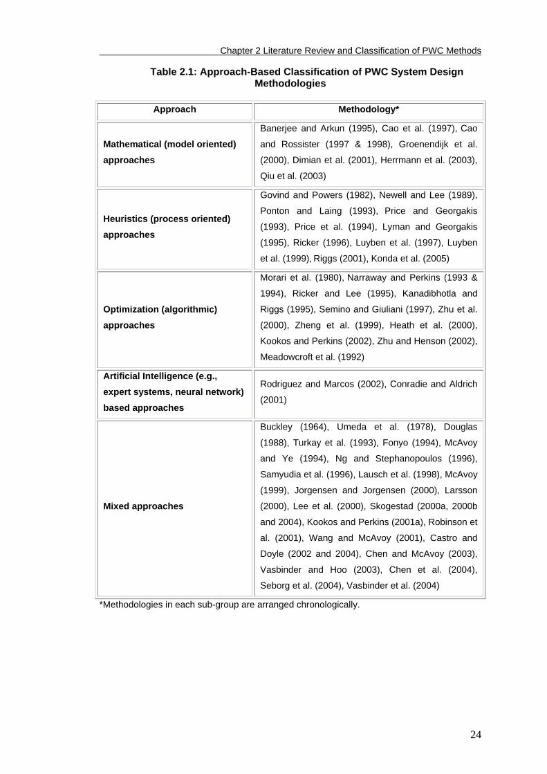
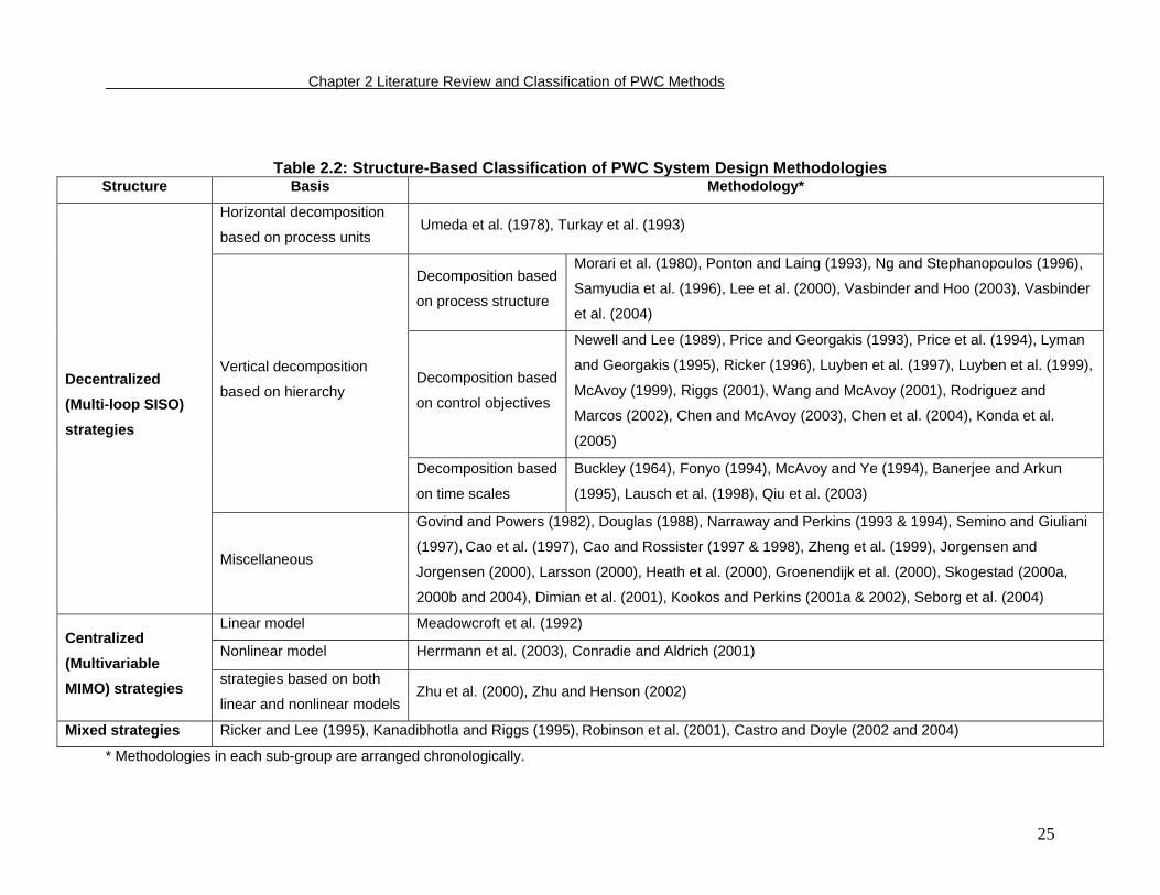
system design studies are classified here in two ways. The first classification is
based on the main approach in the method (approach-based classification in Table
2.1) and the second classification is based on the controller structure adopted
(structure-based classification in Table 2.2). Approach and structure are attributes for
all the methodologies and thus form a good basis for classification.
One recent attempt towards the classification of PWC methodologies is by
Larsson (2000). However, classifications in Tables 2.1 and 2.2 are more
comprehensive and up-to-date. Larsson (2000) addressed only the decentralized
control strategies but not the centralized control strategies. Structure-based
classification in Table 2.2 includes the centralized control strategies as well. In
addition, many recent methodologies, which were not in the Larsson’s classification,
have been included in Tables 2.1 and 2.2. Usually, the mathematical and
optimization approaches are considered alike. However, keeping in view the large
number of such methodologies and the differences in techniques employed in them,
they are classified separately as mathematical and optimization approaches in Table
21
Chapter 2 Literature Review and Classification of PWC Methods
2.1. The mathematical approaches use process models (steady-state and/or
dynamic) along with controllability tools like relative gain array (RGA), Niederlinski
index (NI), singular value decomposition (SVD), condition number (CN), disturbance
condition number (DCN), closed loop disturbance gain (CLDG), relative disturbance
gain (RDG), performance relative gain (PRG) etc. On the other hand, optimization
approaches use numerical methods like MILP, MINLP etc. In this regard, these two
approaches are classified into two different classes.
Classification of PWC system design methodologies is challenging as some
of them might fit into more than one category since they adopt a few approaches
and/or structures. Thus, the subdivisions cannot be considered to be mutually
exclusive. For example, multi-horizon control system of Ng and Stephanopoulos
(1996) employs a hierarchical framework in which the plant is vertically decomposed
into a set of representations of different degrees of abstraction. Starting from the
longest time-horizon of operation (input-output structure), they try to identify and
prioritize the significant control objectives in that representation of the plant, and then
a control system is designed to satisfy these objectives according to their priority in
that level. They then move down to one level of the hierarchy to refine the model and
correspondingly the objectives and control system in order to meet the overall plant
objectives in that shorter time-horizon of operation. This procedure is repeated till the
shortest time-horizon of operation is reached. Therefore, the methodology of Ng and
Stephanopoulos (1996) can be placed in the vertical decomposition based on
process structure or in the vertical decomposition based on control objectives in
Table 2.2. We opted to put this methodology in the former as it places greater
emphasis on vertical decomposition based on process structure. Nevertheless, these
subdivisions provide convenient means to classify various PWC methodologies.
Through these classifications, researchers and engineers can immediately identify
the two main features of any PWC methodology at a glance. It should be noted that,
22

Chapter 2 Literature Review and Classification of PWC Methods
in addition to the references that propose PWC methods, references that merely
apply the proposed methods are also included in these classifications; these
applications (e.g., Lyman and Georgakis (1995); Qiu et al. (2003); Vasbinder et al.
(2004)) demonstrate the general validity of the respective methods and also offer
greater insight.
23
Chapter 2 Literature Review and Classification of PWC Methods
24
Table 2.1: Approach-Based Classification of PWC System Design Methodologies
Approach Methodology*
Mathematical (model oriented) approaches
Banerjee and Arkun (1995), Cao et al. (1997), Cao
and Rossister (1997 & 1998), Groenendijk et al.
(2000), Dimian et al. (2001), Herrmann et al. (2003),
Qiu et al. (2003)
Heuristics (process oriented) approaches
Govind and Powers (1982), Newell and Lee (1989),
Ponton and Laing (1993), Price and Georgakis
(1993), Price et al. (1994), Lyman and Georgakis
(1995), Ricker (1996), Luyben et al. (1997), Luyben
et al. (1999), Riggs (2001), Konda et al. (2005)
Optimization (algorithmic) approaches
Morari et al. (1980), Narraway and Perkins (1993 &
1994), Ricker and Lee (1995), Kanadibhotla and
Riggs (1995), Semino and Giuliani (1997), Zhu et al.
(2000), Zheng et al. (1999), Heath et al. (2000),
Kookos and Perkins (2002), Zhu and Henson (2002),
Meadowcroft et al. (1992)
Artificial Intelligence (e.g., expert systems, neural network) based approaches
Rodriguez and Marcos (2002), Conradie and Aldrich
(2001)
Mixed approaches
Buckley (1964), Umeda et al. (1978), Douglas
(1988), Turkay et al. (1993), Fonyo (1994), McAvoy
and Ye (1994), Ng and Stephanopoulos (1996),
Samyudia et al. (1996), Lausch et al. (1998), McAvoy
(1999), Jorgensen and Jorgensen (2000), Larsson
(2000), Lee et al. (2000), Skogestad (2000a, 2000b
and 2004), Kookos and Perkins (2001a), Robinson et
al. (2001), Wang and McAvoy (2001), Castro and
Doyle (2002 and 2004), Chen and McAvoy (2003),
Vasbinder and Hoo (2003), Chen et al. (2004),
Seborg et al. (2004), Vasbinder et al. (2004)
*Methodologies in each sub-group are arranged chronologically.
Chapter 2 Literature Review and Classification of PWC Methods
25
Table 2.2: Structure-Based Classification of PWC System Design Methodologies Structure Basis Methodology*
Horizontal decomposition
based on process units Umeda et al. (1978), Turkay et al. (1993)
Decomposition based
on process structure
Morari et al. (1980), Ponton and Laing (1993), Ng and Stephanopoulos (1996),
Samyudia et al. (1996), Lee et al. (2000), Vasbinder and Hoo (2003), Vasbinder
et al. (2004)
Decomposition based
on control objectives
Newell and Lee (1989), Price and Georgakis (1993), Price et al. (1994), Lyman
and Georgakis (1995), Ricker (1996), Luyben et al. (1997), Luyben et al. (1999),
McAvoy (1999), Riggs (2001), Wang and McAvoy (2001), Rodriguez and
Marcos (2002), Chen and McAvoy (2003), Chen et al. (2004), Konda et al.
(2005)
Vertical decomposition
based on hierarchy
Decomposition based
on time scales
Buckley (1964), Fonyo (1994), McAvoy and Ye (1994), Banerjee and Arkun
(1995), Lausch et al. (1998), Qiu et al. (2003)
Decentralized (Multi-loop SISO) strategies
Miscellaneous
Govind and Powers (1982), Douglas (1988), Narraway and Perkins (1993 & 1994), Semino and Giuliani
(1997), Cao et al. (1997), Cao and Rossister (1997 & 1998), Zheng et al. (1999), Jorgensen and
Jorgensen (2000), Larsson (2000), Heath et al. (2000), Groenendijk et al. (2000), Skogestad (2000a,
2000b and 2004), Dimian et al. (2001), Kookos and Perkins (2001a & 2002), Seborg et al. (2004)
Linear model Meadowcroft et al. (1992)
Nonlinear model Herrmann et al. (2003), Conradie and Aldrich (2001) Centralized (Multivariable MIMO) strategies strategies based on both
linear and nonlinear modelsZhu et al. (2000), Zhu and Henson (2002)
Mixed strategies Ricker and Lee (1995), Kanadibhotla and Riggs (1995), Robinson et al. (2001), Castro and Doyle (2002 and 2004)
* Methodologies in each sub-group are arranged chronologically.
Chapter 2 Literature Review and Classification of PWC Methods
2.4 Dynamic Modeling and Process Simulators
Control engineers have been using dynamic simulation tools over decades to
study process control concepts and to design control systems. Dynamic models for
some standard unit operations are given in several text books (e.g., Luyben, 1990). Most
of the control studies in the past, however, are based on linear models and/or individual
units. Watson et al. (2000) nicely discussed the problems associated with decisions
based on individual unit simulations, and subsequently highlighted the need to carry out
plant-wide simulations based on a case-study that involves retrofitting a pharmaceutical
plant. However, as stated by Mandler (2000), though SIMULINK can efficiently handle
small scale problems, it is too cumbersome to use SIMULINK for plant-wide simulations;
thus, process simulators, such as SPEEDUP, are more suitable for PWC studies.
Process simulators have a wide range of applications spanning from process
control, operation, troubleshooting and training (Sowa, 1997). For example, Feliu et al.
(2003) have recently demonstrated how such simulators can improve product quality,
productivity and process safety. In addition, they can also be used in startup studies
(e.g., Fabro et al., 2005) and in process optimization (e.g., Jang et al., 2005). However,
despite the expected benefits of these simulators, as stated by Marquardt (1991), they
have not widely been used in the process industry due to several reasons; one of the
main reasons being the significant effort and time needed to setup and analyze rigorous
dynamic models. The situation is slowly changing due to the advancements in
computing technology, object-oriented programming and numerical methods; and these
dynamic simulation tools are evolving into a tool for everyday use by engineers.
Consequently, several dynamic simulation tools, both in-house and commercial, are now
available. For example, Cole and Yount (1994) demonstrated the use of in-house
26
Chapter 2 Literature Review and Classification of PWC Methods
simulation tools to develop and analyze control and safety systems for industrial
processes. Longwell (1994) presented three projects that have resulted in millions of
dollars of economic benefit by improving the plant operability using DuPont’s in-house
simulator, TMODS.
Since early 90’s, several commercial dynamic process simulators (e.g., Aspen
Dynamics, HYSYS) are available with reasonably sophisticated features. Laganier
(1996) presented some applications using commercially available simulation packages
including SpeedUp, HYSYS, Winsim and gPROMS, and discussed their capabilities and
shortcomings. Since then, these simulators have been gradually improved to become
more accurate, robust and user-friendly, and these improvements are expected to
continue due to the continuing research effort in this direction. For example, most of the
existing process simulators are based on differential algebraic equations (DAE). Over
the last decade, there has been increasing attention towards integrating partial
differential algebraic equations (PDAE) in such simulators to further the modeling
accuracy (e.g., Oh and Pantelides, 1996; Martinson and Barton, 2000). Similarly,
simulation tools that can support both the continuous and discrete systems are
becoming available (e.g., Rodriguez, 2005).
Several applications of HYSYS and Aspen Dynamics for control of industrial
processes are discussed by Luyben (2002), while Seider et al. (2004) discussed how
these simulators can be used in process design, control and optimization. Another
notable and one of the most recent dynamic simulation packages is “ForeSee” (Tu and
Rinard, 2006). ForeSee differs from most of the existing dynamic simulators in the way
the equipment models are represented. Existing process simulators model the standard
unit operations. On the other hand, ForeSee has four component models -
27
Chapter 2 Literature Review and Classification of PWC Methods
containments, core models, connectors, and coordinators – which can be combined to
model/simulate standard unit operations. For example, instead of a distillation column
model, ForeSee contains a model of a more fundamental component, i.e., tray, and such
tray models can then be assembled to generate model for a distillation column. In
addition to all the above-mentioned simulation packages, industry-specific process
simulators are also available in order to address particular needs of different process
industries; for example, Polymer Plus and RefSYS can be used to simulate polymer
processes and refineries, respectively. Similarly, simulation packages, such as BATCH-
DIST (Diwekar and Madhavan, 1991), are available to simulate multi-component batch
distillations. Lately, Barrero et al. (2003) discussed the development and testing of
simulation models for power plants, and Chen and Adomaitis (2006) presented
simulation models for semiconductor processes.
Despite the increasing availability of the dynamic process simulators, their usage
in PWC research is rather limited. Out of the many PWC studies presented in the
previous section, only a few are carried out using such rigorous simulators, and thus the
PWC community has not fully explored the power of these simulators. Prompted by
these observations, in this thesis, a commercial process simulator (i.e., HYSYS) is
extensively used to model the HDA process in all the illustrations. HYSYS has many
standard unit operations which are developed using first-principles based models.
Though some standard units, such as rate-based distillation column, membrane and
fluidized bed reactor, are not available in HYSYS, they can be easily modeled using
Visual Basic. Besides, thermodynamic properties (such as vapor-liquid equilibrium) can
be predicted using an extensive collection of traditional property packages, such as
Peng-Robinson (PR) and Non-Random-Two-Liquid (NRTL) equations. If the database is
not available to make use of these methods (e.g., if the binary interaction parameters are
28
Chapter 2 Literature Review and Classification of PWC Methods
not available), newer ones such as conductor-like screening models (COSMO) are now
becoming available which can predict thermodynamic properties based on solvation
thermodynamics and computational quantum mechanics (Mullins et al. 2006). However,
the thermodynamic properties for the components in a conventional petrochemical
process such as the HDA process can be predicted with reasonable accuracy using the
PR model in HYSYS (e.g., Peng and Robinson, 1976); hence, PR model is used in the
present study.
2.5 Summary
Considering the importance and complexity of recycle systems, significant
research has been carried out on recycle dynamics since early 1980s. Following this,
control of recycle systems has been given great deal of attention since late 1980s.
Subsequently, the control of more complex systems (i.e., control of plants with several
recycles - PWC) has been one of the active areas of research in the last 15 years. Due
to the availability of a large number of PWC methods, comprehensive and systematic
classifications are presented in this chapter from which researchers can easily identify
the two important features (i.e., the approach used and the structure employed) of each
method. From Table 2.2, it is evident that relatively more number of methods based on
decentralized multi-loop SISO strategy are available when compared to the number of
methods based on its counterpart, i.e., centralized control strategy; this is mainly due to
the complexity involved in applying the latter to large scale processes. From Table 2.1,
artificial intelligence (AI) based approaches for PWC are rather limited. However, such
approaches can be expected to be available in future due to increasing applicability of AI
techniques.
29
Chapter 2 Literature Review and Classification of PWC Methods
Despite the availability of powerful process simulators, these have not
extensively been used by PWC community. Thus, in this thesis, a commercial process
simulator (i.e., HYSYS) is used to explore and evaluate its potential for PWC studies. In
addition to PWC, other relevant issues like performance assessment of PWC systems
and interaction between design and control from plant-wide perspective are also studied
in Chapters 5 and 6 respectively. Brief review of the literature pertaining to these topics
is given in the respective chapters.
30
Chapter 3 Integrated Framework
CHAPTER 3
INTEGRATED FRAMEWORK OF SIMULATION AND
HEURISTICS*
More effective and efficient PWC methodologies are becoming increasingly
important as chemical processes are becoming more and more integrated with
recycles for reasons of safety, environmental considerations and economics. Hence,
in this chapter, an integrated framework of simulation and heuristics is proposed. The
main emphasis here is on vertical integration of simulation and heuristics which
exploits the inherent interlink between them. By adopting this framework, simulators
can be more efficiently utilized and they also offer invaluable support to the decisions
taken by heuristics. The proposed framework is then successfully applied to the HDA
process. An analysis of results shows that the proposed framework builds synergies
between the powers of both the simulation and the heuristics thereby resulting in a
practical PWC methodology that leads to a viable control system.
3.1 Introduction
Plant-Wide Control: In the past, unit-based control system design
methodology (Umeda et al., 1978) has been widely used to design control systems
for complete plants. However, the recent stringent environmental regulations, safety
concerns and economic considerations, demand the design engineers to make the
chemical processes highly integrated with material and energy recycles. As
discussed in Chapter 2, several researchers studied the effect of these recycles on
the overall dynamics and concluded that recycles need special attention while
* This chapter is based on the paper - Konda, N. V. S. N. M.; Rangaiah, G. P.; Krishnaswamy, P. R. Plant-Wide Control of Industrial Processes: An Integrated Framework of Simulation and Heuristics. Ind. Eng. Chem. Res. 2005, 44, 8300-8313.
31
Chapter 3 Integrated Framework
designing PWC systems as they change the dynamics of the plant in a way which
may not always be apparent from the dynamics of the individual unit-operations.
Hence, the unit-based methodology seems to be scarcely equipped to design the
control system for such complex plants. For example, Downs (1992) reported a
control strategy for a scrubber-distillation column with a liquid recycle which did not
work from an overall point of view, though the control of individual unit operations
was satisfactory. Luyben (2000a) also demonstrated how control decisions vary
based on perception i.e., whether the unit is considered as a single unit-operation or
an integral part of the plant. Thus, there is a need for better methodologies which can
deal with the highly integrated processes in a more efficient way. This leads to the
concept of PWC which demands plant-wide perspective while designing PWC
systems.
Designing control systems for highly integrated processes is challenging
because of the large combinatorial search space. For example, Price and Georgakis
(1993) observed 70 alternative control strategies for a simple hypothetical reactor-
separator process with a single recycle. Keeping in view of this large combinatorial
search space, the ultimate solution may not be so intuitively obvious. So, many
researchers have addressed PWC problem over the last two decades and came up
with various methodologies. After a critical review of various methodologies, the
heuristic-based methodologies are found to be easier not only to understand but also
to implement. However, novices often face difficulties while adopting some of these
heuristics which need experience and basic process understanding for their effective
usage. This problem can be best addressed by using simulation tools such as
HYSYS, which are becoming increasingly popular and can give “virtual hands-on
experience” to novices. Moreover, heuristics cannot always be totally relied upon as
the solution can sometimes be unconventional. In addition, heuristics can sometimes
be contradictory and leave the designer in a dilemma (Douglas, 1985). Motivated by
32
Chapter 3 Integrated Framework
these, we integrated simulation tools and heuristics to develop a simulation-based
heuristic methodology which can handle the PWC problem effectively and
realistically.
Chemical Process Simulators: Although simulation tools have seen
widespread usage in process control related applications in the past, most of these
studies are based on steady state simulation and a few of them are based on
dynamic simulation of individual unit operations with little emphasis on PWC (Tyreus,
1992). It is only around early 1990s that the advent of computer technology permitted
the development of commercial plant-wide dynamic simulators. Since then, the field
of dynamic simulation is rapidly growing and, today, several commercial dynamic
simulators, such as HYSYS Dynamics, which can effectively model large-scale
processes, are available. However, even with the present day advances, using
dynamic simulators, especially for complex applications such as PWC system
design, is not easy. It is just not enough to know the simulators per se. It demands
more than that along with the application of solid engineering principles and
significant amount of time. These issues are much more pronounced especially in the
context of PWC. So, integrating the PWC heuristics with the dynamic simulation
capabilities, as discussed in this chapter, greatly facilitates the PWC system design
and increases use of dynamic simulation.
Some design heuristics and simulation techniques have already evolved as
integrated tools and some of the process design studies are being carried out using
simulators along with the aid of heuristics which proved to be very beneficial. For
example, a designer can save time if the design heuristic: keep the operating reflux
ratio at 1.2 times the minimum reflux ratio is known. Else, the designer would have to
explore a larger search space to find the optimal solution. Applying this heuristic
33
Chapter 3 Integrated Framework
certainly makes the designer’s task easier while simulating and optimizing distillation
columns.
Most of the single unit operation control studies can be done fairly easily by
using dynamic simulation tools. But, the complexities associated with dynamic
simulation tools precluded the application of these tools especially to PWC problems.
Thus, rigorous nonlinear simulation was used in a few studies only to
evaluate/validate the control systems once they are developed. However, the recent
technological advances made the simulation technology mature enough to handle
even the complex problems within a reasonable amount of time (Sowa, 1997).
Moreover, Moore’s law states that the computing speed doubles every 18 months
which in turn nurtures progress in the simulation technology. Hence, simulators are
likely to gain widespread use throughout the process industries and in academia.
With the promise of these improvements in the simulation technology, the PWC
community can benefit by addressing PWC problems with the aid of the simulation
tools.
The remaining chapter is organized as follows: the next section presents an
integrated framework of simulation and heuristics for PWC of industrial processes.
Section 3.3 includes the details of the HDA process and its steady-state modeling
using HYSYS. Application of the proposed methodology to the HDA process and the
resulting control systems’ performance evaluation are presented in section 3.4.
Finally, chapter summary is given in section 3.5.
34
Chapter 3 Integrated Framework
3.2 Proposed Integrated Framework of Simulation and Heuristics
The objective of this section is to develop a unified PWC methodology which
is amenable to study practical concerns in a flexible way which in turn would lead to
the best-practical solution (control system). After a careful review of PWC
methodologies, heuristic-based methodologies are found to be intuitively attractive
because they are easier to understand and implement. Heuristic-based
methodologies just need the basic understanding of the process along with some
experience. So, we have chosen to develop a heuristic-based methodology.
Mathematical tools such as RGA are also used, wherever necessary, to reap more
benefits. Pioneering work in this direction is by Luyben et al. (1999) who proposed a
9-step heuristic procedure. This procedure will be referred as Luyben’s methodology
hereafter. While this methodology does not have any serious limitations, it does have
some shortcomings. For example, Luyben et al. (1999) sub-divided the big task of
designing the overall PWC system into smaller tasks. However, in each step
(especially set production rate and material inventory steps) the decision is ad hoc,
which would impede the usage of this methodology. As the TPM dictates the overall
control system structure and thereby performance, the production rate must be set
carefully. To make the situation worse, production rate is a typical kind of variable for
which one can find many alternatives. Moreover, overall material inventory control is
obviously a plant-wide concern as it must be a self-consistent structure (Price and
Georgakis, 1993). Though a general discussion is given in Luyben et al. (1999)
specific guidelines are not apparent from this discussion. Systematic guidelines at
this stage are essential. So, we adopted the guidelines from Price and Georgakis
(1993) to facilitate the selection of manipulators for the throughput and inventory
regulation.
35
Chapter 3 Integrated Framework
One of the heuristics in Luyben’s methodology is to fix a flow in the recycle
loop to avoid snowball effect, which is popularly known as Luyben’s rule. It gives an
impression that the flow in the recycle loop has to be controlled whenever there is a
recycle. But this need not always necessarily be true. For example, the proposed
integrated framework develops a viable control system (discussed in section 3.4)
which does not require any flow control in the recycle loop. Similar observation was
made by Bildea et al. (2000) and Dimian (2003). The former formulated a
mathematical criterion based on which one can judge when the conventional control
structure can perform better than the control structure developed by applying
Luyben’s rule. Dimian (2003) presented some cases wherein the conventional control
structure can perform better than the control structure developed by applying
Luyben’s rule. Balasubramanian et al. (2003) showed that fixing a flow in the recycle
loop can result in instabilities especially when there are delays which are often the
case in reality. Moreover, snowball effect cannot really be eliminated from the
process by fixing a flow in the recycle loop but it is only transferred from one location
to another (Yu, 1999). So, better alternatives to avoid snowball effect rather than
fixing flow in the recycle loop are needed.
Though Luyben’s methodology (1999) yields viable control structures, some
of them are ‘unbalanced’† control structures which are not desirable. In addition to
this, Luyben’s methodology may yield “self-inconsistent” structures (self-consistency
is discussed in Appendix A). Though these structures may be workable control
strategies, extensive simulation studies by Price and Georgakis (1993) have shown
that they are inferior to self-consistent structures in terms of performance. There are
other issues (especially in complex integrated processes) that are not intuitive. As
† If there is any disturbance affecting the process, flow rates of all streams in the process will have to vary according to material balances. But, fixing a flow in the recycle loop forces the control system to act on the system to reach a forced steady state in which one or more units need to take more rigorous action than others. This kind of control structures is called unbalanced control structure (Yu, 1999).
36
Chapter 3 Integrated Framework
these issues can be best addressed by dynamic simulation, dynamic simulation and
heuristics are integrated to find a practical solution. In every level/stage, nonlinear
steady-state and dynamic models of the plant are used to take the decision or to
support the decision suggested by heuristics. A few reported studies on PWC are
based on steady-state models. One of the major downsides of these methodologies
is that the steady-state feasibility of the process does not guarantee the plant-wide
controllability. In addition, steady-state analysis might not be adequate for control
studies all the time (Skogestad and Jacobsen, 1990). So, dynamic simulation should
be more emphasized especially in the context of PWC.
The improved heuristic methodology consists of eight levels (Table 3.1).
Various steps involved along with the role of simulation models in each step of the
methodology are discussed below.
Level 1:
Define PWC Objectives: PWC objectives should be formulated from the operational
requirements of the plant. These control objectives typically include product quality,
production rate, stable operation of the plant, process and equipment constraints,
safety concerns and environmental regulations. Many a times, there can be
disagreement between the plant-wide objectives and unit operations objectives. For
example, the best local control decisions (in the context of single units), may have
long-range effects throughout the plant (Stephanopoulos and Ng, 2000). In this case,
the plant-wide objectives should be given priority as ultimately the plant as a whole
should operate properly. Considerable attention need to be paid while defining the
PWC objectives as the control system decisions are dictated more by the underlying
operating objectives than the control performance (Downs, 1992).
37
Chapter 3 Integrated Framework
Role of Simulation Models: All the objectives can be set by process requirements.
Coming to the objectives related to the process stability, the question at this stage is
whether the process is operating at stable steady-state or not. This can be answered
by the steady-state and dynamic simulation models. For example, in the case of feed
effluent heat exchanger with a plug flow reactor, the steady-state simulation model
with and without energy recycle can be perturbed to see whether it is converging to
the same values in both the cases. If so, one can conclude that the process is
operating at stable operating conditions; otherwise, the process is operating at
unstable steady-state. Dynamic simulation models can also be used to check
whether the process is stable or not (i.e., by checking the process variables’
responses are bounded or not). The dynamic stability is guaranteed later in Level 4.
Determine CDOF: Luyben et al. (1999) proposed to count the number of control
valves to find the CDOF of the process. This is true but not a practical solution at this
stage because, many a times, it is the job of the control engineer to place the control
valves in the process flow diagram which needs the knowledge of CDOF of the
process. That means the CDOF is a priori information that needs to be known before
the placement of control valves. Accordingly, control valves can be placed in
strategic locations in the plant. Else, it may so happen that more or less control
valves may be placed if the engineer is not familiar with the plumbing rules. These
kinds of problems occur more frequently if the process is highly integrated. If more
valves are placed, the process would be less economical due to the increased power
requirements for compressors and pumps. On the other hand, if fewer valves are
placed, all the control objectives cannot be achieved or, at times, the process can
even become uncontrollable.
Traditionally, CDOF is obtained by subtracting the sum of number of
equations and externally defined variables from the number of variables (Seborg et
38
Chapter 3 Integrated Framework
al., 2004; Seider et al., 2004). This procedure is impractical for highly integrated
plants and prone to error (Seborg et al., 2004, p. 238). Ponton (1994) proposed a
method for CDOF by counting the number of streams and subtracting the number of
extra phases (i.e., if there are more than one phase present in that unit). However,
simple examples can easily be constructed where this method fails. For example,
CDOF for a heater/cooler remains the same irrespective of the number of phases
involved in the unit. Larrson (2000) also observed some cases wherein Ponton’s
(1994) method fails. So, a simpler and accurate procedure to calculate the CDOF will
be more useful; such a procedure is proposed and discussed in detail in Chapter 4.
For the time being, it is assumed that the information about CDOF is available (e.g.,
by counting the number of valves in the process).
Level 2: Unlike many works, full PWC system design problem including the
parametric decisions (tuning parameters) is addressed here. Hence, the following
issues are mandatory.
Identify and Analyze Plant-Wide Disturbances: It is important to have a notion
about the nature of disturbances expected along with their sources, magnitude and
also how they propagate through the plant as they have considerable impact on the
selection of control structure (Moore, 1992; Price and Georgakis, 1993; Marlin, 1995)
and controller tuning. For example, Price and Georgakis (1993) observed different
control structures performing differently for different disturbances.
Role of Simulation Models: Expected disturbances can be tried out on the steady-
state simulation model to observe how the effect of the disturbances is propagating
throughout the plant; While trying out various disturbances on the steady-state
simulation model, one must make sure that the specifications given are appropriate.
This analysis would be useful later while tuning the controllers. For example,
39
Chapter 3 Integrated Framework
anticipated disturbances can have more severe effects at some sections of the plant
and hence the controllers in these sections should be tuned more conservatively to
make all the sections of the plant equally robust. This is one of the important
requirements that arises from plant-wide perspective, and is confirmed from our
extensive simulations - the most sensitive sections in the plant required relatively
more conservative tuning for good rejection of the disturbances studied.
Set Performance and Tuning Criteria: This step should be considered before any
structural/parametric decisions as performance criteria have considerable impact on
structural/parametric decisions. For example, Price et al. (1994) showed that control
structure may differ with the performance criteria chosen. Setting an unanimous
performance criterion for the overall plant control system is a challenging task as
there can be many loops of different dynamics. For example, one would prefer quick
settling for fast-responding loops like levels and will go for P-only controllers where
off-set is not very important. On the other hand, one would prefer zero offset for slow-
responding loops like composition. To make the situation worse, it is not only the kind
of loop but also the location of the loop also dictates the performance criteria. For
example, in the case of level control, one cannot always go for averaging control; one
will have to go for less conservative tuning if the level is in a distillation column and
the performance criteria would also depend on the control structure selected. Control
structure for distillation bottoms composition and reboiler level is a good example
wherein the performance criteria change with the control structure considered; if the
column base level is controlled by reboiler heat input and bottoms composition is
controlled by bottoms flow, then the level control should be tightly tuned since it is
nested inside the composition loop which otherwise would have been tuned
conservatively (Luyben, 2002).
40
Chapter 3 Integrated Framework
Performance criteria such as integral error can be considered but analysis
would be much more difficult. Hence, in the preliminary stages, settling time (not the
normalized settling time is used in the initial screening stage; more rigorous analysis
is carried out during the final selection of control system, as will be discussed in
chapters 5 and 6) is considered as the performance criterion (while making sure that
all the process objectives and constraints are satisfied) for highly complicated
processes with dozens of control loops involved. Integral error can be chosen as the
performance criterion for more rigorous studies in later stages. Performance
assessment of PWC systems is the subject of Chapter 5; and a measure to gauge
the plant-wide dynamic performance based on rigorous and nonlinear simulation is
proposed in Chapter 5. As the improved heuristic methodology is integrated with
dynamic simulation, the controller needs to be tuned once the structural decision
regarding that particular loop is taken.
Role of Simulation Models: Simulation tools are very useful for tuning. Often,
preliminary tuning of flow, level and pressure loops is a trivial task and can be done
fairly easily based on standard guidelines (Luyben, 2002). But composition and
temperature loops need careful tuning. Making use of built-in tools in dynamic
simulators is effective; for example, auto-tuning (closed loop relay-feedback
technique) can be used to estimate good initial controller settings. One of the
advantages of auto-tuning is that it can also be used for open-loop unstable systems
if there exists a stable limit cycle (Yu, 1999).
Level 3: Structural decisions regarding product specifications should be taken even
before considering the process stability which is the basic criterion of any control
system.
Production Rate Manipulator Selection: This involves identifying the primary
process path (from main raw material to main product). Many primary process paths
41
Chapter 3 Integrated Framework
may exist when there are several raw materials and products. Each primary process
path may be considered to develop alternatives if the best one cannot be found at
this stage. After identification of the primary process path, internal/implicit variables
on this path are preferred as the throughput manipulators (TPMs) over
external/explicit variables (fixed-feed or on-demand) as the former are found to be
dynamically more effective (Price and Georgakis, 1993). The former are usually
associated with the reactor operating conditions. Between fixed-feed or on-demand
options, the former is preferred over the latter as it is shown to be superior in terms of
performance (Price and Georgakis, 1993; Luyben, 1999).
Role of Simulation Models: The dynamic simulation model cannot be made use of
to take the decision about the TPM at this stage as the overall control strategy is not
yet in place. But, as a good starting point, one can make use of steady-state
simulation model to choose the primary process path. Some processes may have
multiple inputs and outputs with several reactions taking place in the reactor, in which
case this procedure will be of great use. For example, for processes involving
dominant side reactions the most intuitive TPM (e.g., limiting reactant flow rate) may
not be the best. After selecting the primary process path, the TPM can be selected
along this line by using a steady-state simulation model. Obviously the one with
maximum steady state gain will be the preliminary choice as the TPM.
Product Quality Manipulator Selection: In this step, one selects the manipulated
variable (MV) for product quality. Other composition loops, if any, will be dealt with
after the material inventory loops (levels) are taken care of as the latter respond
faster and so better handles need to be reserved for levels. In addition, as most of
the levels are integrating (non-self-regulating), level loops need to be given priority
over composition loops as stability concerns are associated with levels. Hence, other
composition loops will be dealt in level 5 (control of unit operations).
42
Chapter 3 Integrated Framework
Role of Simulation Models: This stage deals with product purity, which is often a
local decision; i.e., manipulator for product quality can be found in/around the unit
with which the product stream is associated (Luyben, 1993). Though the product
quality is a local decision, it has to be considered before other plant-wide decisions
(such as material inventory and component balances) because of its ultimate
importance. The unit producing the product stream can be separately simulated for
selecting the best manipulator for product quality. Other structural decisions that are
taken for simulating the unit need not be the best from the overall plant point of view
and so these decisions need not be carried forward to the next levels except the
product quality manipulator.
Level 4:
Selection of Manipulators for More Severe Controlled Variables: Process
constraints such as equipment and operating constraints, safety concerns and
process stability issues will be dealt with in this stage as they have severe operability
implications.
Role of Simulation Models: Dynamic simulation model can be made use of to
choose the best manipulators for meeting severe process constraints. Good initial
estimates for the tuning parameters can also be obtained using in-built tools of the
simulator such as auto tuning.
Selection of Manipulators for Less Severe Controlled Variables: Levels need to
be taken care of while ensuring that the levels in the primary process path are self-
consistent (Appendix A). Other levels that are not in the primary process path should
be controlled in such a way that the control will direct the disturbances away from the
43
Chapter 3 Integrated Framework
primary process path. Last, pressures (often self-regulating in nature) need to be
controlled.
Role of Simulation Models: Level loops are placed so that they will form a self-
consistent structure. Process knowledge from simulation must also be used while
taking the decisions based on heuristics. Decision supported by simulation must be
chosen in the case of any conflict because heuristics need not always be true.
Finally, pressure loops can be placed with the aid of dynamic simulation models. In
highly integrated processes, with long gas-processing lines, it is often difficult to
decide whether to control the pressure at a particular location or not. For example, in
the TE process, it is often adequate to control the pressure of the vapor in an entire
section of the process by using a manipulator at a single location and allowing the
remaining vapor inventories to float, if the pressure drops in the gas loop are small.
Dynamic simulation model would be of great use while taking this decision.
Level 5:
Control of Unit Operations: Control of individual unit operations is considered prior
to checking component material balances. By doing so, some of the component
inventory loops will be implicitly taken care of in this stage thereby making the
analysis in the next stage (checking component inventory) easier.
Role of Simulation Models: At this level, all the individual unit operations can be
simulated. This step mainly deals with the composition loops (or temperature loops)
as all other loops (levels and pressures) have already been taken care of in the
earlier stages. While placing the control loops on individual unit operations one must
ensure that the plant-wide objectives are not violated (for example, one can simulate
different disturbance scenarios with the primary units in the process to see if any of
44
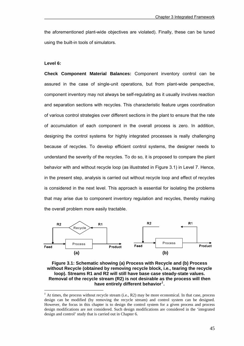
Chapter 3 Integrated Framework
the aforementioned plant-wide objectives are violated). Finally, these can be tuned
using the built-in tools of simulators.
Level 6:
Check Component Material Balances: Component inventory control can be
assured in the case of single-unit operations, but from plant-wide perspective,
component inventory may not always be self-regulating as it usually involves reaction
and separation sections with recycles. This characteristic feature urges coordination
of various control strategies over different sections in the plant to ensure that the rate
of accumulation of each component in the overall process is zero. In addition,
designing the control systems for highly integrated processes is really challenging
because of recycles. To develop efficient control systems, the designer needs to
understand the severity of the recycles. To do so, it is proposed to compare the plant
behavior with and without recycle loop (as illustrated in Figure 3.1) in Level 7. Hence,
in the present step, analysis is carried out without recycle loop and effect of recycles
is considered in the next level. This approach is essential for isolating the problems
that may arise due to component inventory regulation and recycles, thereby making
the overall problem more easily tractable.
Process
Recycle
Feed Product
R1R2
ProcessFeed Product
R1R2
Process
Recycle
Feed Product
R1R2
Process
Recycle
Feed Product
R1R2
ProcessFeed Product
R1R2
ProcessFeed Product
R1R2
(a) (b)
Figure 3.1: Schematic showing (a) Process with Recycle and (b) Process without Recycle (obtained by removing recycle block, i.e., tearing the recycle
loop). Streams R1 and R2 will still have base case steady-state values. Removal of the recycle stream (R2) is not desirable as the process will then
have entirely different behavior‡. ‡ At times, the process without recycle stream (i.e., R2) may be more economical. In that case, process design can be modified (by removing the recycle stream) and control system can be designed. However, the focus in this chapter is to design the control system for a given process and process design modifications are not considered. Such design modifications are considered in the ‘integrated design and control’ study that is carried out in Chapter 6.
45
Chapter 3 Integrated Framework
Role of Simulation Models: In simulation, flow rates of all components at various
locations can be accessed. Using these along with reaction stoichiometry to account
for generation and consumption of components via reactions, accumulation tables
can be prepared to check whether the rate of accumulation is zero while the plant
without recycle loops is in operation (i.e., while the simulation is running). If there is
any accumulation, process topology must be analyzed carefully to ensure that some
component inventory loops are not forgotten. In some complex processes, it is
difficult to ensure that all the inventory loops are in place. So, one can make use of
simulation to ensure that all the inventory loops are placed according to the process
requirements.
Level 7:
Effects due to Integration: This step needs to be analyzed only after all the above
issues (in the previous steps) have been taken care of. Luyben et al. (1999)
considered this step in the earlier stages. Their reasoning is that the plant-wide
decisions need to be given higher priority and therefore need to be satisfied in the
earlier stages. But the hierarchy should ideally be based on how severe the
integration effects are from a plant-wide perspective. One can argue that, if found to
be very severe based on the steady-state analysis, this step can be done earlier and
Luyben’s rule can be applied. However, in this case, the probability of arriving at
unbalanced structures and self-inconsistent structures would be higher, which is not
desirable. Besides, from our tests with simulators, it is observed that there is an
inherent interlink between component inventory regulation and introduction of
recycles. It would thus be easier and more appropriate to analyze them in
consecutive steps. Hence, it is better to analyze the integration effects at the end and
take appropriate action. There are no solid guidelines at this stage except making
use of rigorous simulation models to design a workable control strategy. It would give
46
Chapter 3 Integrated Framework
the control engineer flexibility to choose the better one which otherwise would have
been eliminated by applying some heuristics. Note that Luyben’s rule is not rejected
here but considered as one of the potential alternatives based on necessity, rather
than as a rule.
Role of Simulation Models: To understand the severity of the recycle dynamics, the
process with and without the recycles should be simulated for anticipated
disturbances § . Typically, the process with the recycles exhibits slower (or even
unstable) dynamics. If not, the recycle dynamics can be concluded as not severe. In
the case of slower or unstable dynamics, the control structure has to be altered either
by including additional control loops or by revising the control decisions that have
been taken in the earlier stages. Decision making at this stage is going to be
process-specific and hence cannot be generalized. One can try out the two
suggestions in the improved heuristic methodology (Table 3.1). These guidelines
need not necessarily result in a control system with satisfactory performance and
stability requirements. In such a case, rigorous simulation can be used to
troubleshoot the process. Needless to say, the decisions in the earlier stages need to
be revised, if a workable control strategy cannot be generated at this stage. Finally,
one can simulate and evaluate the performance of alternative control structures, if
any, to find the best.
Level 8:
Enhance Control System Performance, if possible: The designer can look into
possible modifications to further enhance the performance of the control system. For
example, one can look into re-configuring the loops or re-structuring the control
§ Since there can be several recycles, this analysis can be carried out sequentially (i.e., one disturbance at a time) to gauge the impact of respective recycle on the overall process dynamics. Throughput changes (with different magnitudes) should be considered in this analysis since they are not only the most common type of disturbances but they also severaly affect the overall process dynamics.
47
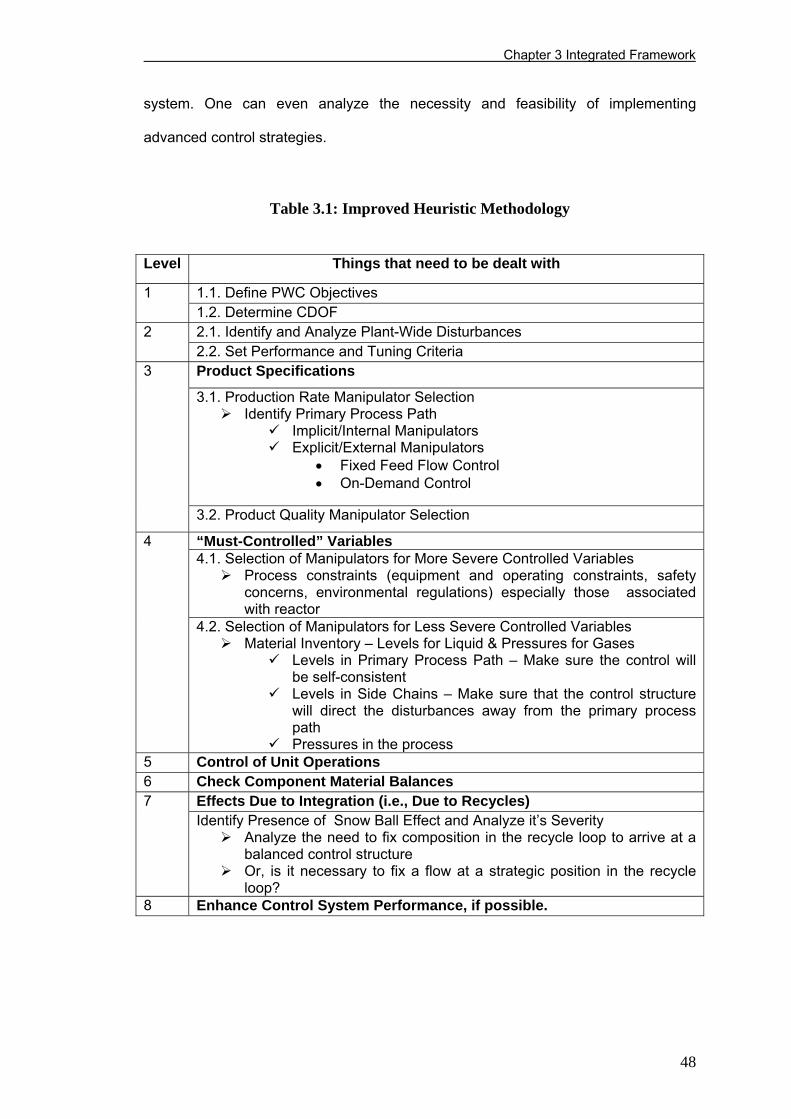
Chapter 3 Integrated Framework
system. One can even analyze the necessity and feasibility of implementing
advanced control strategies.
Table 3.1: Improved Heuristic Methodology
Level Things that need to be dealt with
1.1. Define PWC Objectives 1 1.2. Determine CDOF 2.1. Identify and Analyze Plant-Wide Disturbances 2 2.2. Set Performance and Tuning Criteria Product Specifications
3.1. Production Rate Manipulator Selection Identify Primary Process Path
Implicit/Internal Manipulators Explicit/External Manipulators
• Fixed Feed Flow Control • On-Demand Control
3
3.2. Product Quality Manipulator Selection
“Must-Controlled” Variables 4.1. Selection of Manipulators for More Severe Controlled Variables
Process constraints (equipment and operating constraints, safety concerns, environmental regulations) especially those associated with reactor
4
4.2. Selection of Manipulators for Less Severe Controlled Variables Material Inventory – Levels for Liquid & Pressures for Gases
Levels in Primary Process Path – Make sure the control will be self-consistent
Levels in Side Chains – Make sure that the control structure will direct the disturbances away from the primary process path
Pressures in the process 5 Control of Unit Operations 6 Check Component Material Balances
Effects Due to Integration (i.e., Due to Recycles) 7 Identify Presence of Snow Ball Effect and Analyze it’s Severity
Analyze the need to fix composition in the recycle loop to arrive at a balanced control structure
Or, is it necessary to fix a flow at a strategic position in the recycle loop?
8 Enhance Control System Performance, if possible.
48
Chapter 3 Integrated Framework
The proposed integrated framework is clearly more detailed on how to go
about the PWC problem and can be applied to any industrial process. The framework
is logically developed and has several new features as indicated below:
• Heuristics-based methodology is improved with more specific and useful
guidelines wherever necessary.
• The sequence in Luyben’s heuristics-based methodology is altered to facilitate
the use of rigorous nonlinear simulation models and also to make the PWC
problem more tractable. For example, severity of the recycle dynamics is
systematically analyzed, to take necessary corrective action, towards the end
(i.e., in the 7th stage).
• Several studies in the past used dynamic simulation to validate and evaluate
alternative control system designs after they are developed. On the other hand,
the proposed framework integrates heuristics and simulation models at each
stage of the procedure (and not simply at the end) to achieve greater insight. This
has several benefits.
• The rigorous simulation models are very useful in gauging and screening
any of the heuristics thereby resulting in more efficient control system(s).
• The proposed framework is likely to reduce the number of alternative
control systems (by screening un-attractive alternatives at each stage)
that need to be evaluated at the end thereby making the overall task
easier.
• The integrated framework will be very useful to novices as simulation
models offer virtual hands-on experience, while the heuristics serve as
guidelines to design effective control systems.
• The framework will increase applications of dynamic simulation of process
plants, which is often not possible without a basic regulatory control
system.
49
Chapter 3 Integrated Framework
3.3 Overview and Simulation of the HDA Process
The most widely utilized test-beds for the PWC studies are the TE plant
(Downs, 1993) and the classical reactor-separator-recycle section. These have been
proved to be beneficial for the PWC community to better understand the PWC
problems. However, there is a need to study additional processes which are of
practical importance (i.e., typical industrial processes with real components and
many standard unit operations) and complex enough (with material and energy
recycles) to be representative in its essential features as PWC applications. So, we
have chosen the HDA process which is a highly integrated and nonlinear
petrochemical process. The presence of heat integrated adiabatic plug flow reactor
(PFR) with exothermic reactions and three multi-component, high purity distillation
columns and high level of interaction (because of the presence of material and
energy recycles) makes it really a challenging process for control system design.
Some reported studies on the HDA process are by Luyben et al. (1999) and Qiu et al.
(2003).
3.3.1 HDA Process Description
In the HDA process, fresh toluene (pure) and hydrogen (H2) – i.e., 95% H2
and 5% methane, (CH4) - are mixed with recycled toluene and H2 (Figure 3.2). This
reactant mixture is preheated in a feed-effluent heat exchanger (FEHE) using the
reactor effluent stream and then heated to the reaction temperature in a furnace
before being fed to the adiabatic PFR. Two main reactions taking place inside this
reactor are:
50
Chapter 3 Integrated Framework
Toluene + H2 → Benzene + CH4
2 Benzene ↔ Diphenyl + H2
The reactor effluent is quenched with a portion of the recycle separator liquid to
prevent coking, and further cooled in the FEHE and cooler before being fed to the
flash separator. A portion of unconverted H2 and CH4 overhead vapor from the
separator is purged (to avoid accumulation of CH4 within the process) while the
remainder is compressed and recycled to the reactor. The liquid from the separator is
processed in the separation section consisting of three distillation columns. The
stabilizer column removes H2 and CH4 as the overhead product, and benzene is the
desired product from the product column top. Finally, in the recycle column, toluene
is separated from diphenyl, as the distillate and recycled back.
3.3.2 Steady-State Simulation
The success of any steady-state simulation model largely depends on the
selection of a suitable thermodynamic package (Carlson, 1996; Horwitz and Nocera,
1996; Benyahia, 2000). In this study, the improved Peng-Robinson (PR) equation of
state is selected for property estimation as it is very reliable for predicting the
properties of hydrocarbon-based components over a wide range of conditions and is
generally recommended for oil, gas and petrochemical applications. With the use of
default templates in HYSYS, the steady-state simulation model of the HDA process
has been developed according to the flow-sheet topology (Figure 3.2) and the
process information from Douglas (1988). Though Douglas (1988) considered 75%
as the optimal conversion, recent studies by Phimister et al. (1999) showed that the
optimal conversion is 70% and hence the base case HDA process flowsheet is
developed based on 70% conversion. This variation is not unexpected and can be
qualitatively explained based on the variation in the feedstock and utility prices since
1988.
51
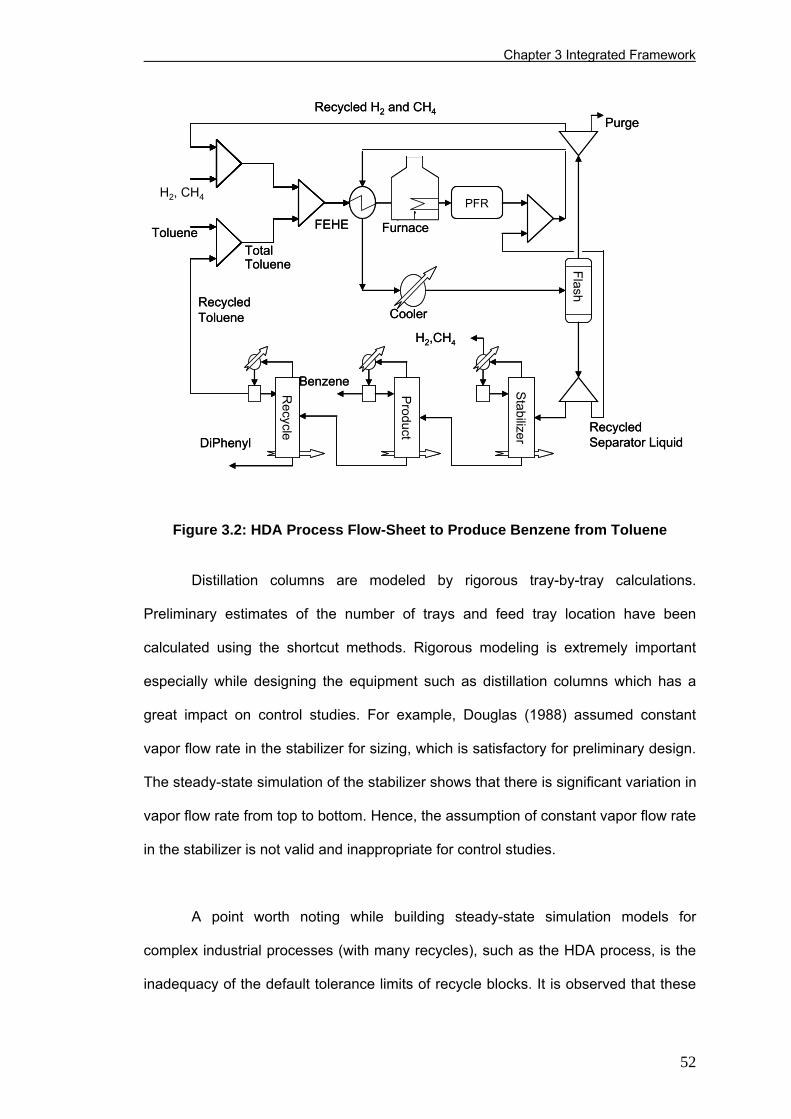
Chapter 3 Integrated Framework
Toluene
Purge
H2, CH4
Product
Stabilizer
PFRFlash
FEHE Furnace
DiPhenyl
Benzene
H2,CH4
Cooler
Recycle
Recycled H2 and CH4
Recycled Toluene
Recycled Separator Liquid
Total Toluene
Toluene
Purge
H2, CH4
Product
Stabilizer
PFRFlash
FEHE Furnace
DiPhenyl
Benzene
H2,CH4
Cooler
Recycle
Recycled H2 and CH4
Recycled Toluene
Recycled Separator Liquid
Total Toluene
Figure 3.2: HDA Process Flow-Sheet to Produce Benzene from Toluene
Distillation columns are modeled by rigorous tray-by-tray calculations.
Preliminary estimates of the number of trays and feed tray location have been
calculated using the shortcut methods. Rigorous modeling is extremely important
especially while designing the equipment such as distillation columns which has a
great impact on control studies. For example, Douglas (1988) assumed constant
vapor flow rate in the stabilizer for sizing, which is satisfactory for preliminary design.
The steady-state simulation of the stabilizer shows that there is significant variation in
vapor flow rate from top to bottom. Hence, the assumption of constant vapor flow rate
in the stabilizer is not valid and inappropriate for control studies.
A point worth noting while building steady-state simulation models for
complex industrial processes (with many recycles), such as the HDA process, is the
inadequacy of the default tolerance limits of recycle blocks. It is observed that these
52
Chapter 3 Integrated Framework
default tolerance limits fail to give reasonably accurate results. This causes
accumulation in the process which in turn makes the initial transients longer in
dynamic simulation as we can use the same steady-state model in dynamic mode
also with some modifications. So, we need to pay considerable attention to the
recycle tolerances to get reasonably accurate results. Not only the recycle tolerance
limits, but the number of recycles and the location of recycle blocks also affect the
computational efficiency. Thus, in general, recycles pose convergence difficulties
while developing steady-state simulation models (e.g., Schad, 1994 and 1998).
However, such problems can be resolved by making use of “recycle assistant”, which
is an added feature in the newer versions of HYSYS (i.e., Aspen HYSYS 2004 or
later versions). Recycle assistant aids the user to place the recycles in strategic
locations in such a way that the number of recycles can be minimized, and thus the
convergence can be achieved in less number of iterations.
3.3.3 Moving from Steady-State to Dynamic Simulation
HYSYS provides an integrated steady-state and dynamic simulation
capability. In this integrated simulation environment, the dynamic model shares the
same physical property packages and flow-sheet topology as the steady-state model.
Thus, it is easy to switch from steady-state to dynamic mode. However, there are
several differences in both these environments in terms of specifications and solution
methodology. One major difference is the pressure drop in distillation columns; a
constant value has to be specified for this in steady-state mode whereas it will be
calculated in dynamic mode based on the given tray data. So, while moving to the
dynamic mode, a systematic procedure of many steps, namely, plumbing, Pressure-
Flow (P-F) specifications and equipment sizing, needs to be followed, which are
briefly discussed below (Luyben, 2002).
53
Chapter 3 Integrated Framework
Plumbing: To take care of some of the dynamic effects introduced in the dynamic
mode, the flow-sheet topology may have to be modified by placing the additional
units such as pumps wherever necessary and this is called plumbing. One of the
important steps in plumbing is placement and sizing of the control valves in the
process. For realistic dynamic simulations, the “plumbing” in the flow-sheet should be
appropriately done to ensure the flow of material from one unit to another.
P-F specifications: In dynamic mode, we need to give additional specifications
besides the usual steady-state specifications (for material and energy balance
calculations). These additional specifications are known as P-F specifications. The
numerical integration technique that is used to solve the resulting equations in
dynamic mode is implicit Euler method with fixed step-size. Usually pressure
specifications are preferred over flow specifications as the “pressure-driven” mode of
simulation is more realistic, especially for the processes in which the hydraulics and
fluid mechanics are of vital importance. However, in some cases flow specifications
need to be given.
Equipment Sizing: As the dynamics of any unit is dependent on size of the
equipment, various units (e.g., distillation columns) need to be sized before moving to
dynamic mode which can be done using in-built tools such as tray sizing utility.
In principle, we can then switch over to dynamic mode at this stage. However,
considering the complex nature of the highly integrated processes with several
recycles, open-loop dynamic simulation of the entire process may not be possible
and/or useful for analysis due to the overlapping effects of many phenomena. Thus, it
is advisable to place at least some key loops before running any plant-wide dynamic
simulations. For example, if there is any problem while simulating, it is difficult to
identify whether the problem is due to improper specification(s) or inefficiency of the
54
Chapter 3 Integrated Framework
control system. So, proper guidelines are necessary at this stage to resolve this
problem. This is where heuristics can aid us to proceed further via a step by step
systematic procedure. Both the steady-state and dynamic simulation models are
made use of to integrate simulation with the proposed improved heuristic
methodology to design the PWC system for the HDA process in the following section.
It should be noted that all the dynamic simulations in this and also in the subsequent
chapters are carried out without any noise.
3.4 Application of Proposed Methodology to the HDA Process
The dynamic simulation model of the HDA process consists of 959 nonlinear,
highly coupled algebraic and differential equations. This part of the study would also
reveal the capability of dynamic simulation in the context of PWC.
Step 1.1: Define PWC Objectives
1. Production Rate - 280 lb mol of benzene/hour (9.92 tonnes/hour)
2. Product Quality - Benzene purity ≥ 99.97%
3. Process Stability - The feed effluent heat exchanger with plug flow reactor has
been simulated and perturbed with and without heat integration, and the results
reveal that the process with heat integration is operating at unstable steady-
state. It has also been observed that maintaining the reactor inlet temperature
at a constant value stabilizes the process.
4. Process Constraints (Douglas, 1988):
• The temperature at the reactor inlet should be around 1150 oF. This is an
optimization decision to have better reaction rates.
• The ratio of H2 to aromatics (i.e., benzene, toluene, and biphenyl) has to be
at least 5 at the inlet. This is basically to provide a thermal sink to avoid
55
Chapter 3 Integrated Framework
coking that takes place at higher temperatures. Also, excess H2 encourages
the primary reaction and discourages the secondary reaction (Smith, 1995).
• The temperature at the reactor outlet should not exceed 1300 oF to avoid
coking.
• The outlet stream from the reactor must be quenched to 1150 oF to prevent
thermal decomposition of products and to avoid fouling in FEHE.
Step 1.2: Determine CDOF
Available CDOF is found to be 23 (Luyben, 1999).
Step 2.1: Identify and Analyze the Plant-Wide Disturbances
The important plant-wide disturbances in the HDA process are ± 25%
variation in toluene feed rate, - 2.5% variation in H2 feed purity and ± 5% variation in
the set-point of flash drum level. From the steady-state simulation model, it is
observed that 5% variation in the toluene feed flow rate produced a large variation,
up to 20% in the flows of separation section; and, 85% variation is observed in the
separation section flows for 25% variation in the toluene feed flow rate. This
information will be useful while taking tuning decisions in the next step.
Step 2.2: Set Performance and Tuning Criteria
Settling time is chosen as the performance criterion for the preliminary
studies. The analysis in the previous step showed that small variations in the toluene
feed flow rate produced larger variations in the flows of separation section. So,
separation section controllers must be more conservatively tuned compared to those
in other parts of the plant.
56
Chapter 3 Integrated Framework
Step 3.1: Production Rate Manipulator Selection
From steady-state simulation, the steady-state gain of toluene to benzene is
found to be much larger than that of H2 to benzene. So, the primary process path can
be selected as toluene to benzene (Figure 3.2). As reactor conversion is an
optimization decision, reactor conditions (internal TPMs) like temperature etc., cannot
be used as the TPMs. So, the next best alternative i.e., fixed-feed flow of toluene, is
considered as the TPM. Jorgensen and Jorgensen (2000) reported that the H2 feed
stream is the better TPM than the toluene feed stream. Their contention is that the
toluene as the TPM fails to account for the side reaction and increasing the H2
concentration limits the extent of side reaction leading to better selectivity and higher
production rate. At first sight, Jorgensen and Jorgensen’s (2000) argument seems to
be alright. However, it fails to take into consideration the extent of reactions. From
the steady-state simulation, it can be seen that the extent of side reaction is
negligible when compared to that of the main reaction. In this regard, toluene would
still be a better TPM because of its larger gain.
Step 3.2: Product Quality Manipulator Selection
Based on RGA analysis (Svrcek et al., 2000) of the benzene column, it is
found that both the reflux flow and the distillate flow are equally good for controlling
the composition of benzene in the product stream. Hence, the conventional structure
with reflux as the manipulator for product quality is selected.
Step 4.1: Selection of Manipulators for More Severe Controlled Variables
The reactor inlet temperature is controlled by furnace duty and the PFR with
FEHE is observed to be stable in the dynamic mode. Here the decision is quite
straightforward. But in certain cases (e.g., if we consider bypass to FEHE) dynamic
simulation can be used to make the decision. The initial estimates for the tuning
parameters are calculated using the auto-tuning tool in HYSYS Dynamics. The
57
Chapter 3 Integrated Framework
second process constraint is on the H2-to-aromatics ratio at the reactor inlet. So, H2
feed is selected to maintain the ratio of H2 to aromatics into the rector. In this case, it
turns out to be a quite straightforward decision. It is implemented as a ratio control
using spreadsheet available in HYSYS Dynamics. In the control strategy of Luyben et
al. (1999), there is no explicit control of H2 to aromatics ratio. However, it is advisable
to handle the process constraints explicitly as in our case. The H2-to-toluene ratio has
been considered in the previous studies whereas the actual process constraint is on
the ratio of H2 to aromatics (McKetta, 1977). This constraint is very important as there
can be coking if the H2 to aromatics ratio is less than five and the process will not be
economically attractive if the ratio is more than five. So, it is most advisable to have
an explicit control over this process constraint.
The third process constraint is to maintain the outlet temperature of the
reactor within 1300 0F. From the steady-state simulation model, it can be seen that
the reactor outlet temperature (1220.1 0F) is well below 1300 0F. So, this is an
inactive process constraint (even in the presence of worst-case disturbance) and an
explicit control action is not needed. The last process constraint is to quench the
reactor effluent stream to 1150 0F. From the process knowledge, the most intuitive
manipulator is the quench stream from the flash drum.
Step 4.2: Selection of Manipulators for Less Severe Controlled Variables
Levels in the primary process path are controlled in the direction of flow (as
fixed feed flow is the TPM) to have self-consistent structure (Appendix A and Figure
A.1). But there is one unavoidable exception to this; the toluene column condenser
level should not be controlled by distillate stream as it back-propagates the
disturbances to primary process path. But the other immediate alternative, reflux flow
as the manipulator, is very inadequate as the reflux ratio is very small (L/D = 0.05).
This compelled us to violate the heuristic. Levels that are in side paths are controlled
58
Chapter 3 Integrated Framework
in such a way that the disturbances are directed away from the primary process path.
Again, there is an exception here; according to this guideline, the toluene column
reboiler level must be controlled by bottoms flow. Fonyo (1994) also considered
bottoms flow as the manipulator for toluene column reboiler level which appears to
be quite obvious. But dynamic simulations showed that the reboiler duty affects the
reboiler level more than the bottoms flows and hence is a better MV for reboiler level
control in the toluene column. This can be intuitively explained based on the fact that
the reboil (boil-up) ratio is very high (~ 24) and bottoms flow rate (i.e., biphenyl) is
very small (as the selectivity losses towards biphenyl for the base case HDA process
are considerably low). These two examples show that the heuristics cannot always
be relied upon. The heuristics simplify the overall task but they need to be applied
with a good dose of engineering judgment and process-specific knowledge.
Finally, operating pressures of three distillation columns, and flash drum
pressure are controlled appropriately. One interesting issue is the decision regarding
pressure control in the gas line. When the process, such as the HDA process, has a
very long gas line with many unit operations, it is difficult to decide the number of
points at which the pressure needs to be controlled and their strategic locations. In
this case, dynamic simulation can be used. For the HDA process, dynamic simulation
showed that controlling the pressure in the flash drum would ensure the pressure
control in the total gas line. Reactor pressure does not require any explicit control
action.
Step 5: Control of Individual Unit Operations
In this step, all unit operations are analyzed and control loops are placed
wherever necessary. Dual composition control for all the three distillation columns is
considered as it is relatively more optimal than the single end composition control
and also offers better control from the plant-wide perspective. For example, for the
59
Chapter 3 Integrated Framework
recycle column as an individual unit-operation, single end composition control should
be sufficient as the main objective is not to lose toluene from the bottom stream.
However, from a plant-wide perspective minimizing the disturbance propagation
through the recycle stream is also as important as minimizing the toluene loss which
results in dual-composition control. Hence, plant-wide perception is given due
importance and dual-composition control is chosen for the recycle column.
Flash drum inlet temperature has to be controlled which can be achieved by
the duty of the cooler before the flash. In some cases, there exists a strong
correlation between temperature and pressure of an adiabatic flash. In these cases,
either the temperature or the pressure can only be controlled. In the HDA case, the
correlation is not strong and it is preferable to control both for better performance. So,
flash temperature is also controlled.
Step 6: Check Component Balances
All the individual unit operations in the process are simulated separately and,
from the component inventory tables, it is observed that the inventory of all
components in all the units is regulated. However, there is no guarantee that the
component inventory will be regulated when all the units are put together as there
can be incompatibility among the control actions of different controllers. Hence, all
the units are put together according to process topology (without gas and liquid
recycles) and component inventory is observed to be regulated.
Step 7: Effects due to Integration
So far, the analysis is carried out without gas and liquid recycles (i.e., by
tearing both the gas and liquid recycle streams as in Figure 3.1). All the control
decisions that have been taken so far lead to a control system which is stable even
with both the recycles. This control system is same as the one developed by Ponton
60
Chapter 3 Integrated Framework
and Laing (1993). Though they have qualitatively discussed the superiority of their
control system over the control system designed by Stephanopoulos (1984), they did
not report any simulation results to show the performance of their control system.
Moreover, there is no additional consideration for recycles in the analysis of Ponton
and Laing (1993). As shown in the following analysis, a better control system is
generated by systematically analyzing the effect of recycles on overall plant
dynamics.
Effect of Gas Recycle on Overall Plant Dynamics: The closed-loop dynamic
simulation is run with each of the expected disturbances for the HDA process with
and without gas recycle, and the effect of gas recycle on the overall plant dynamics is
observed to be negligible when compared to that of liquid recycle (discussed in the
following section). Possible reasons for this are as follows: (1) gas recycle dynamics
are usually faster than liquid recycle dynamics; (2) any variation in the gas recycle
can easily be attenuated by the H2/aromatics ratio controller; (3) the liquid recycle
dynamics in the HDA process (Figure 3.2), are more complex compared to the gas
recycle dynamics because of the presence of three distillation columns with nonlinear
dynamics. Hence, further analysis is carried out based solely on the impact of liquid
recycle dynamics on the overall dynamics. This can further be justified based on an
analogy from reaction engineering: the slowest of all (parallel) reactions is the rate
limiting step and the analysis can be carried out by ignoring faster reactions.
The gas recycle also contains a purge stream to avoid accumulation of CH4 in
the process and, hence, a composition controller (CC) is needed to make the CH4
inventory in the process self-regulating. The composition of the purge stream is
controlled by manipulating recycle gas flow as it is the larger of the two potential
manipulators available - gas recycle and purge flows. So, composition loop is placed
by making use of the compressor duty as the manipulator, which in turn manipulates
61
Chapter 3 Integrated Framework
62
the gas recycle flow rate. This strategy is equivalent to manipulating steam flow rate
to control gas flow rate in the case of a steam turbine driven centrifugal compressor.
This strategy is the most energy-efficient (Luyben, 2002) and hence implemented in
our study. Alternatively, gas recycle stream can be manipulated by compressor
suction throttling (or bypassing) or purge flow rate manipulation which in turn affects
the gas recycle flow rate to control purge composition.
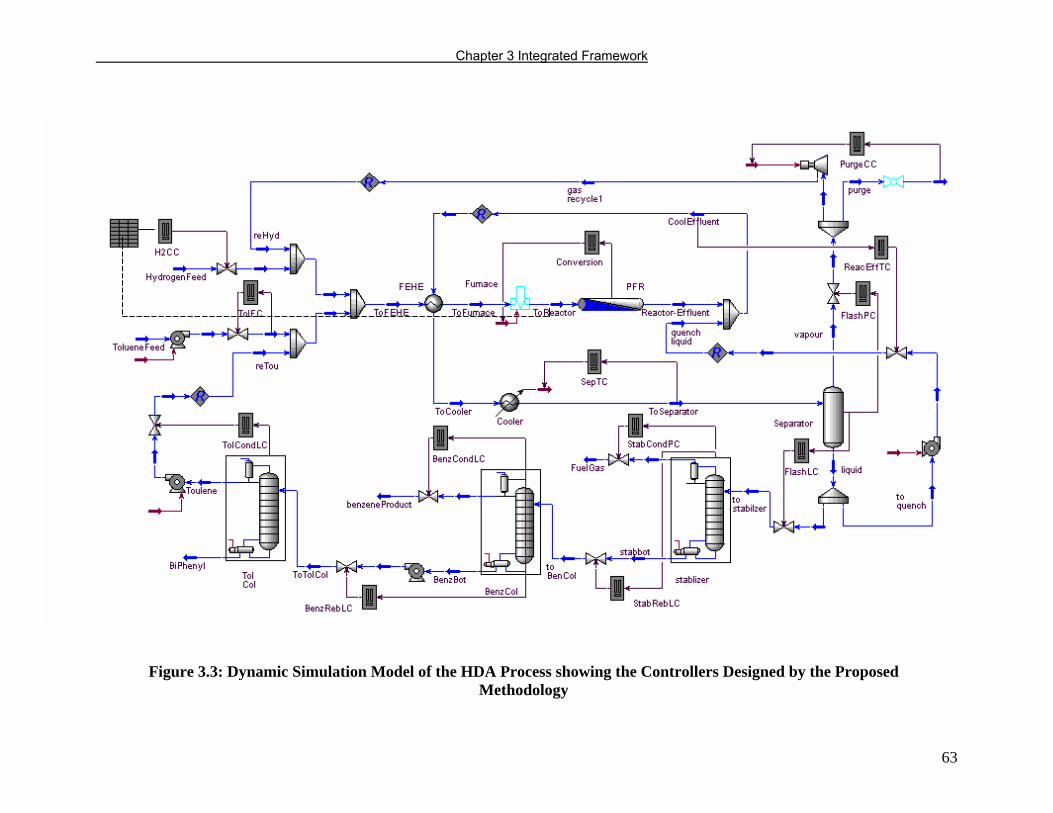
Chapter 3 Integrated Framework
63
Figure 3.3: Dynamic Simulation Model of the HDA Process showing the Controllers Designed by the Proposed Methodology
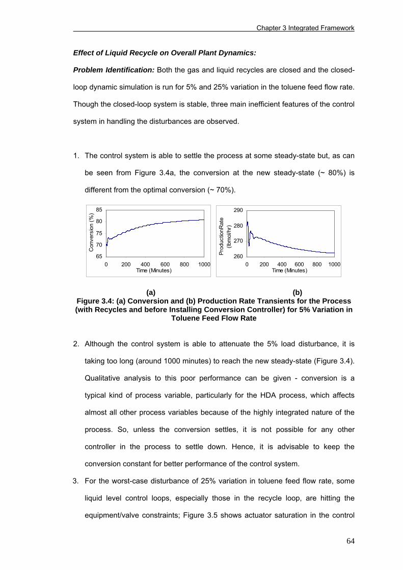
Chapter 3 Integrated Framework
Effect of Liquid Recycle on Overall Plant Dynamics:
Problem Identification: Both the gas and liquid recycles are closed and the closed-
loop dynamic simulation is run for 5% and 25% variation in the toluene feed flow rate.
Though the closed-loop system is stable, three main inefficient features of the control
system in handling the disturbances are observed.
1. The control system is able to settle the process at some steady-state but, as can
be seen from Figure 3.4a, the conversion at the new steady-state (~ 80%) is
different from the optimal conversion (~ 70%).
65
70
75
80
85
0 200 400 600 800 1000Time (Minutes)
Con
vers
ion
(%)
260
270
280
290
0 200 400 600 800 1000Time (Minutes)
Prod
uctio
nRat
e(lb
mol
/hr)
(a) (b) Figure 3.4: (a) Conversion and (b) Production Rate Transients for the Process (with Recycles and before Installing Conversion Controller) for 5% Variation in
Toluene Feed Flow Rate
2. Although the control system is able to attenuate the 5% load disturbance, it is
taking too long (around 1000 minutes) to reach the new steady-state (Figure 3.4).
Qualitative analysis to this poor performance can be given - conversion is a
typical kind of process variable, particularly for the HDA process, which affects
almost all other process variables because of the highly integrated nature of the
process. So, unless the conversion settles, it is not possible for any other
controller in the process to settle down. Hence, it is advisable to keep the
conversion constant for better performance of the control system.
3. For the worst-case disturbance of 25% variation in toluene feed flow rate, some
liquid level control loops, especially those in the recycle loop, are hitting the
equipment/valve constraints; Figure 3.5 shows actuator saturation in the control
64
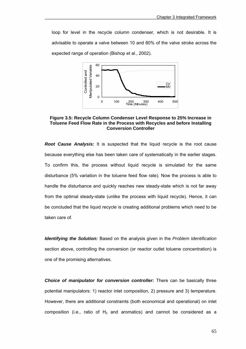
Chapter 3 Integrated Framework
loop for level in the recycle column condenser, which is not desirable. It is
advisable to operate a valve between 10 and 80% of the valve stroke across the
expected range of operation (Bishop et al., 2002).
0
20
40
60
0 100 200 300 400 500Time (Minutes)
Con
trolle
d an
d M
anip
ulat
ed V
aria
ble
CVMV
Figure 3.5: Recycle Column Condenser Level Response to 25% Increase in Toluene Feed Flow Rate in the Process with Recycles and before Installing
Conversion Controller
Root Cause Analysis: It is suspected that the liquid recycle is the root cause
because everything else has been taken care of systematically in the earlier stages.
To confirm this, the process without liquid recycle is simulated for the same
disturbance (5% variation in the toluene feed flow rate). Now the process is able to
handle the disturbance and quickly reaches new steady-state which is not far away
from the optimal steady-state (unlike the process with liquid recycle). Hence, it can
be concluded that the liquid recycle is creating additional problems which need to be
taken care of.
Identifying the Solution: Based on the analysis given in the Problem Identification
section above, controlling the conversion (or reactor outlet toluene concentration) is
one of the promising alternatives.
Choice of manipulator for conversion controller: There can be basically three
potential manipulators: 1) reactor inlet composition, 2) pressure and 3) temperature.
However, there are additional constraints (both economical and operational) on inlet
composition (i.e., ratio of H2 and aromatics) and cannot be considered as a
65
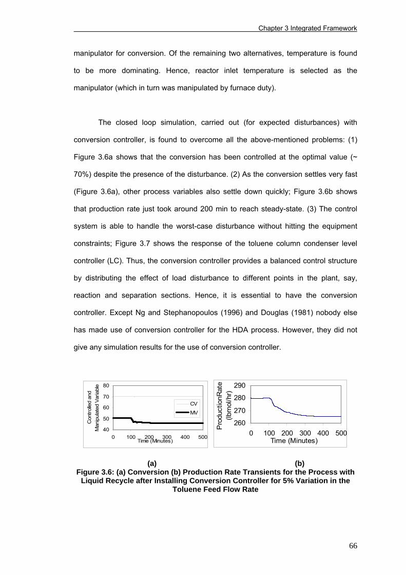
Chapter 3 Integrated Framework
manipulator for conversion. Of the remaining two alternatives, temperature is found
to be more dominating. Hence, reactor inlet temperature is selected as the
manipulator (which in turn was manipulated by furnace duty).
The closed loop simulation, carried out (for expected disturbances) with
conversion controller, is found to overcome all the above-mentioned problems: (1)
Figure 3.6a shows that the conversion has been controlled at the optimal value (~
70%) despite the presence of the disturbance. (2) As the conversion settles very fast
(Figure 3.6a), other process variables also settle down quickly; Figure 3.6b shows
that production rate just took around 200 min to reach steady-state. (3) The control
system is able to handle the worst-case disturbance without hitting the equipment
constraints; Figure 3.7 shows the response of the toluene column condenser level
controller (LC). Thus, the conversion controller provides a balanced control structure
by distributing the effect of load disturbance to different points in the plant, say,
reaction and separation sections. Hence, it is essential to have the conversion
controller. Except Ng and Stephanopoulos (1996) and Douglas (1981) nobody else
has made use of conversion controller for the HDA process. However, they did not
give any simulation results for the use of conversion controller.
40
50
60
70
80
0 100 200 300 400 500Time (Minutes)
Con
trolle
d an
d M
anip
ulat
ed V
aria
ble
CV
MV
260
270
280
290
0 100 200 300 400 500Time (Minutes)
Pro
duct
ionR
ate
(lbm
ol/h
r)
(a) (b) Figure 3.6: (a) Conversion (b) Production Rate Transients for the Process with
Liquid Recycle after Installing Conversion Controller for 5% Variation in the Toluene Feed Flow Rate
66
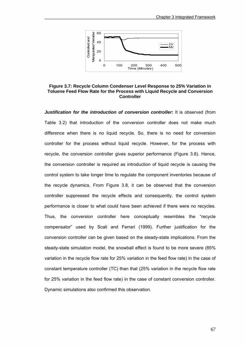
Chapter 3 Integrated Framework
0
20
40
60
0 100 200 300 400 500Time (Minutes)
Con
trolle
d an
d M
anip
ulat
ed V
aria
ble
CVMV
Figure 3.7: Recycle Column Condenser Level Response to 25% Variation in
Toluene Feed Flow Rate for the Process with Liquid Recycle and Conversion Controller
Justification for the introduction of conversion controller: It is observed (from
Table 3.2) that introduction of the conversion controller does not make much
difference when there is no liquid recycle. So, there is no need for conversion
controller for the process without liquid recycle. However, for the process with
recycle, the conversion controller gives superior performance (Figure 3.8). Hence,
the conversion controller is required as introduction of liquid recycle is causing the
control system to take longer time to regulate the component inventories because of
the recycle dynamics. From Figure 3.8, it can be observed that the conversion
controller suppressed the recycle effects and consequently, the control system
performance is closer to what could have been achieved if there were no recycles.
Thus, the conversion controller here conceptually resembles the “recycle
compensator” used by Scali and Ferrari (1999). Further justification for the
conversion controller can be given based on the steady-state implications. From the
steady-state simulation model, the snowball effect is found to be more severe (85%
variation in the recycle flow rate for 25% variation in the feed flow rate) in the case of
constant temperature controller (TC) than that (25% variation in the recycle flow rate
for 25% variation in the feed flow rate) in the case of constant conversion controller.
Dynamic simulations also confirmed this observation.
67
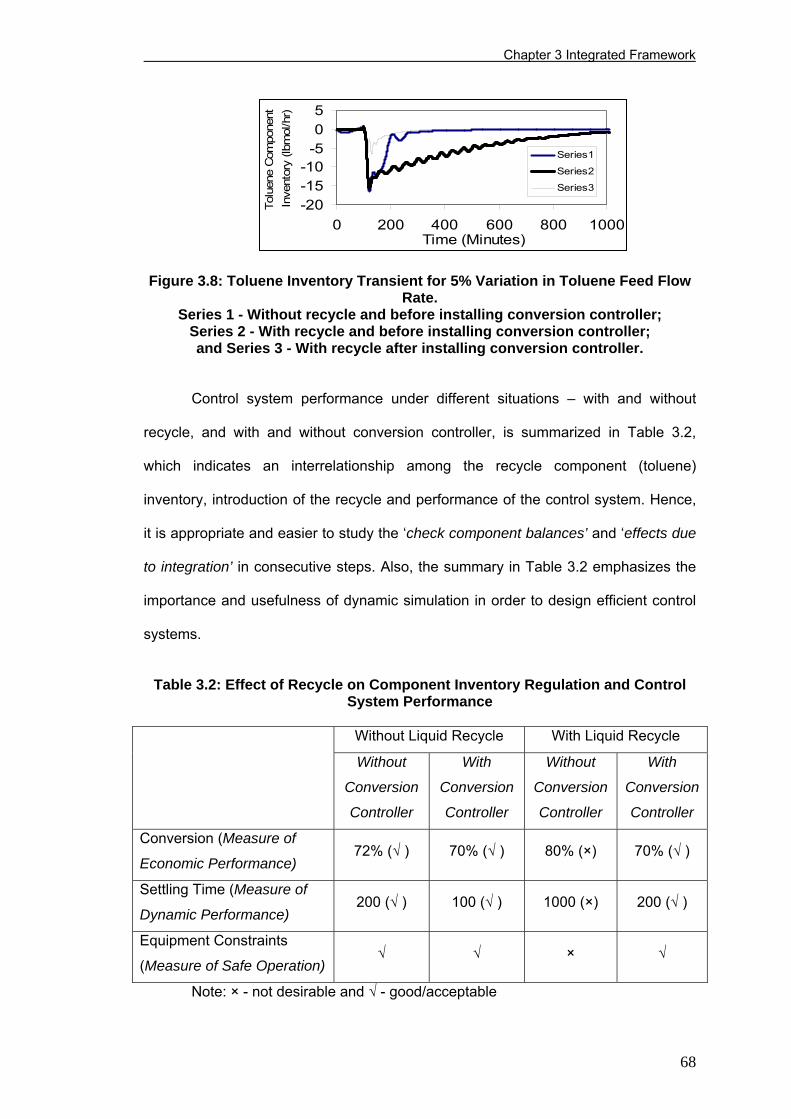
Chapter 3 Integrated Framework
-20-15-10
-505
0 200 400 600 800 1000Time (Minutes)
Tolu
ene
Com
pone
nt
Inve
ntor
y (lb
mol
/hr)
Series1
Series2
Series3
Figure 3.8: Toluene Inventory Transient for 5% Variation in Toluene Feed Flow Rate.
Series 1 - Without recycle and before installing conversion controller; Series 2 - With recycle and before installing conversion controller; and Series 3 - With recycle after installing conversion controller.
Control system performance under different situations – with and without
recycle, and with and without conversion controller, is summarized in Table 3.2,
which indicates an interrelationship among the recycle component (toluene)
inventory, introduction of the recycle and performance of the control system. Hence,
it is appropriate and easier to study the ‘check component balances’ and ‘effects due
to integration’ in consecutive steps. Also, the summary in Table 3.2 emphasizes the
importance and usefulness of dynamic simulation in order to design efficient control
systems.
Table 3.2: Effect of Recycle on Component Inventory Regulation and Control
System Performance
Without Liquid Recycle With Liquid Recycle
Without
Conversion
Controller
With
Conversion
Controller
Without
Conversion
Controller
With
Conversion
Controller
Conversion (Measure of
Economic Performance) 72% (√ ) 70% (√ ) 80% (×) 70% (√ )
Settling Time (Measure of
Dynamic Performance) 200 (√ ) 100 (√ ) 1000 (×) 200 (√ )
Equipment Constraints
(Measure of Safe Operation) √ √ × √
Note: × - not desirable and √ - good/acceptable
68
Chapter 3 Integrated Framework
3.5 Evaluation of the Control System
The control system designed for the HDA process has 23 control loops
(Figure 3.3). The complete plant with this control system but without any disturbance
is simulated for 100 mins. The set point, process variable and controller output of all
the control loops are reported in Table 3.3, which shows that all the process variables
are maintained close to their set-points. In the absence of the disturbances, we
usually expect the controller output near 50% valve opening as they are designed for
50% opening at steady-state base case conditions. However, this is not so for some
loops in Table 3.3 because pressures at different nodes in the dynamic mode are
calculated by pressure-flow solver whereas they are specified in steady-state mode.
This leads to some pressure variations within the process in the dynamic mode when
compared to the steady-state mode. So, there is small offset from 50% in some of
the valve openings as they depend on the neighboring pressures also. The LC in the
flash drum (No. 1, FlashLC controller in Table 3.3) has settled at 68.71% opening
because of liquid choking (flashing) inside the valve.
Various disturbances (load and set-point variations) are now introduced, and
the transient responses of some important process variables are given in Figures 3.9
to 3.13 to show the effectiveness of the control system. It can be seen that the
control system is able to attenuate the disturbances in reasonable settling time,
which varies depending on the nature of the loop (Figures. 3.9 to 3.13).
69
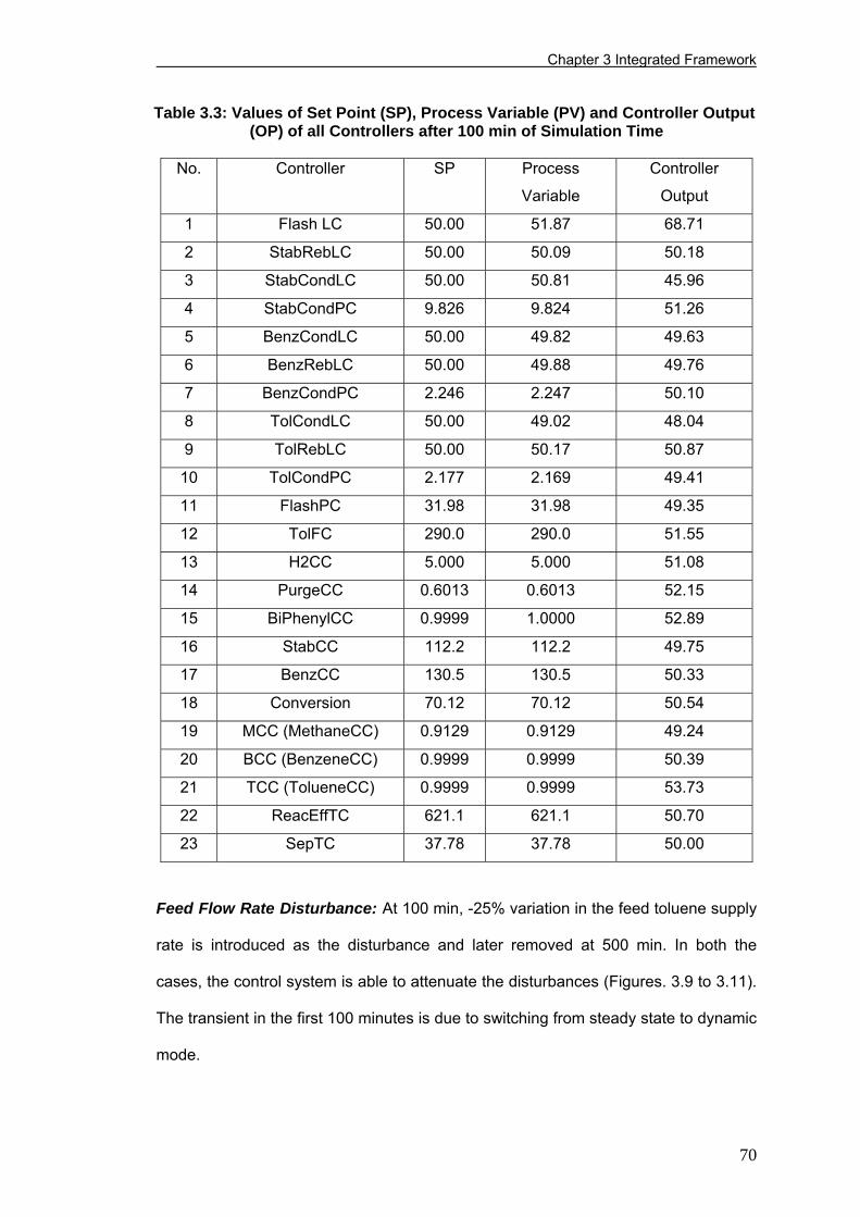
Chapter 3 Integrated Framework
Table 3.3: Values of Set Point (SP), Process Variable (PV) and Controller Output (OP) of all Controllers after 100 min of Simulation Time
No. Controller SP Process
Variable
Controller
Output
1 Flash LC 50.00 51.87 68.71
2 StabRebLC 50.00 50.09 50.18
3 StabCondLC 50.00 50.81 45.96
4 StabCondPC 9.826 9.824 51.26
5 BenzCondLC 50.00 49.82 49.63
6 BenzRebLC 50.00 49.88 49.76
7 BenzCondPC 2.246 2.247 50.10
8 TolCondLC 50.00 49.02 48.04
9 TolRebLC 50.00 50.17 50.87
10 TolCondPC 2.177 2.169 49.41
11 FlashPC 31.98 31.98 49.35
12 TolFC 290.0 290.0 51.55
13 H2CC 5.000 5.000 51.08
14 PurgeCC 0.6013 0.6013 52.15
15 BiPhenylCC 0.9999 1.0000 52.89
16 StabCC 112.2 112.2 49.75
17 BenzCC 130.5 130.5 50.33
18 Conversion 70.12 70.12 50.54
19 MCC (MethaneCC) 0.9129 0.9129 49.24
20 BCC (BenzeneCC) 0.9999 0.9999 50.39
21 TCC (TolueneCC) 0.9999 0.9999 53.73
22 ReacEffTC 621.1 621.1 50.70
23 SepTC 37.78 37.78 50.00
Feed Flow Rate Disturbance: At 100 min, -25% variation in the feed toluene supply
rate is introduced as the disturbance and later removed at 500 min. In both the
cases, the control system is able to attenuate the disturbances (Figures. 3.9 to 3.11).
The transient in the first 100 minutes is due to switching from steady state to dynamic
mode.
70
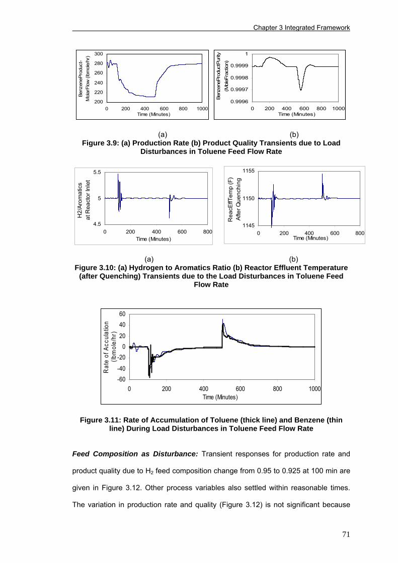
Chapter 3 Integrated Framework
200
220
240
260
280
300
0 200 400 600 800 1000Time (Minutes)
Benz
eneP
rodu
ct-
Mol
arFl
ow (l
bmol
e/hr
)
0.9996
0.9997
0.9998
0.9999
1
0 200 400 600 800 1000Time (Minutes)
Benz
eneP
rodu
ctPu
rity
(Mol
eFra
ctio
n)
(a) (b) Figure 3.9: (a) Production Rate (b) Product Quality Transients due to Load
Disturbances in Toluene Feed Flow Rate
1145
1150
1155
0 200 400 600 800Time (Minutes)
Rea
cEffT
emp
(F)
Afte
r Que
nchi
ng
4.5
5
5.5
0 200 400 600 800Time (Minutes)
H2/
Aro
mat
ics
at R
eact
or In
let
(a) (b) Figure 3.10: (a) Hydrogen to Aromatics Ratio (b) Reactor Effluent Temperature
(after Quenching) Transients due to the Load Disturbances in Toluene Feed Flow Rate
-60-40
-200
20
4060
0 200 400 600 800 1000Time (Minutes)
Rat
e of
Acc
ulat
ion
(lbm
ole/
hr)
Figure 3.11: Rate of Accumulation of Toluene (thick line) and Benzene (thin line) During Load Disturbances in Toluene Feed Flow Rate
Feed Composition as Disturbance: Transient responses for production rate and
product quality due to H2 feed composition change from 0.95 to 0.925 at 100 min are
given in Figure 3.12. Other process variables also settled within reasonable times.
The variation in production rate and quality (Figure 3.12) is not significant because
71
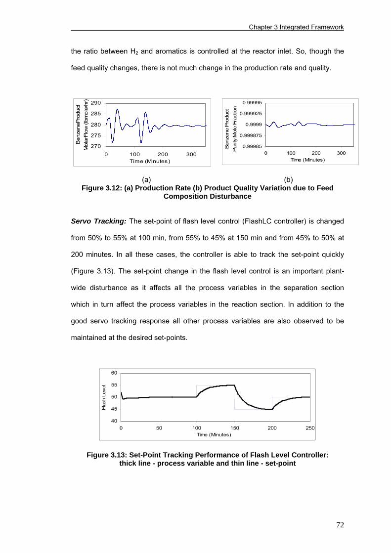
Chapter 3 Integrated Framework
the ratio between H2 and aromatics is controlled at the reactor inlet. So, though the
feed quality changes, there is not much change in the production rate and quality.
0.99985
0.999875
0.9999
0.999925
0.99995
0 100 200 300Time (Minutes)
Ben
zene
Pro
duct
Pu
rity
Mol
e Fr
actio
n
270
275
280
285
290
0 100 200 300Time (Minutes)
Benz
eneP
rodu
ct
Mol
arFl
ow (l
bmol
e/hr
)
(a) (b) Figure 3.12: (a) Production Rate (b) Product Quality Variation due to Feed
Composition Disturbance
Servo Tracking: The set-point of flash level control (FlashLC controller) is changed
from 50% to 55% at 100 min, from 55% to 45% at 150 min and from 45% to 50% at
200 minutes. In all these cases, the controller is able to track the set-point quickly
(Figure 3.13). The set-point change in the flash level control is an important plant-
wide disturbance as it affects all the process variables in the separation section
which in turn affect the process variables in the reaction section. In addition to the
good servo tracking response all other process variables are also observed to be
maintained at the desired set-points.
40
45
50
55
60
0 50 100 150 200 250Time (Minutes)
Flas
h Le
vel
Figure 3.13: Set-Point Tracking Performance of Flash Level Controller: thick line - process variable and thin line - set-point
72
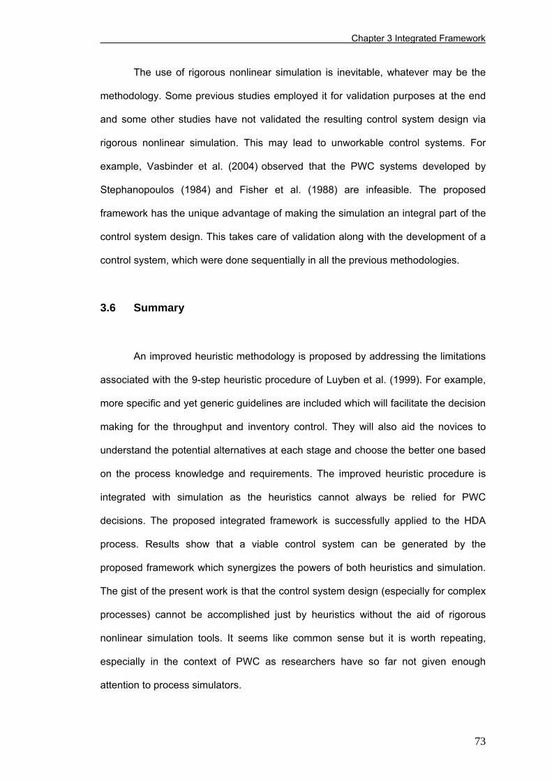
Chapter 3 Integrated Framework
The use of rigorous nonlinear simulation is inevitable, whatever may be the
methodology. Some previous studies employed it for validation purposes at the end
and some other studies have not validated the resulting control system design via
rigorous nonlinear simulation. This may lead to unworkable control systems. For
example, Vasbinder et al. (2004) observed that the PWC systems developed by
Stephanopoulos (1984) and Fisher et al. (1988) are infeasible. The proposed
framework has the unique advantage of making the simulation an integral part of the
control system design. This takes care of validation along with the development of a
control system, which were done sequentially in all the previous methodologies.
3.6 Summary
An improved heuristic methodology is proposed by addressing the limitations
associated with the 9-step heuristic procedure of Luyben et al. (1999). For example,
more specific and yet generic guidelines are included which will facilitate the decision
making for the throughput and inventory control. They will also aid the novices to
understand the potential alternatives at each stage and choose the better one based
on the process knowledge and requirements. The improved heuristic procedure is
integrated with simulation as the heuristics cannot always be relied for PWC
decisions. The proposed integrated framework is successfully applied to the HDA
process. Results show that a viable control system can be generated by the
proposed framework which synergizes the powers of both heuristics and simulation.
The gist of the present work is that the control system design (especially for complex
processes) cannot be accomplished just by heuristics without the aid of rigorous
nonlinear simulation tools. It seems like common sense but it is worth repeating,
especially in the context of PWC as researchers have so far not given enough
attention to process simulators.
73
Chapter 3 Integrated Framework
As a result of the application of the proposed integrated framework to the
HDA process, it is seen that the conversion controller improves the overall
performance. Though conversion controller appears to be somewhat less common, it
is not uncommon in petrochemical processes. For instance, Turkay et al. (1993)
proposed to use conversion controllers for all the three reactors in styrene
manufacturing process to improve the PWC system performance.
74
Chapter 4 Control Degrees of Freedom
CHAPTER 4
A SIMPLE AND EFFECTIVE PROCEDURE FOR CONTROL
DEGREES OF FREEDOM*
The focus of this chapter is on one of the important steps in designing PWC
systems, namely, CDOF. There appears to be no simple procedure to compute
CDOF, the maximum number of flows that can be manipulated simultaneously,
especially in the context of PWC of industrial processes. Hence, a simple and yet
effective procedure to find CDOF is proposed and illustrated in this work. The key
idea is to define 'restraining number' (i.e., the minimum number of flows that can’t be
manipulated along with others in an unit, which is also an inherent characteristic of
that unit) of an unit. We show that the restraining number is equal to the number of
independent and overall material balances with no associated inventory† in that
particular unit. The concept of restraining number is then used to find CDOF of not
only simple units but also highly integrated processes. One of the advantages is its
generic nature, which facilitates its automation. Moreover, the proposed procedure
implicitly takes care of number of phases and components involved in the unit. In
addition, the proposed procedure needs just the basic understanding of simple units
and one does not require all the mathematical equations involved.
* This chapter is based on the paper - Konda, N. V. S. N. M.; Rangaiah, G. P.; Krishnaswamy, P. R. A Simple and Effective Procedure for Control Degrees of Freedom. Chem. Eng. Sci. 2006, 61 (4), 1184-1194. † Inventory is used here to refer to ‘variable hold-up’ but not ‘fixed hold-up’. For example, gas phase (or gas-liquid phase) PFR is considered as the ‘unit with inventory’ as it contains ‘variable hold-up’ and liquid phase PFR is considered as the ‘unit without inventory’ as it contains ‘fixed hold-up’.
75
Chapter 4 Control Degrees of Freedom
4.1 Introduction
CDOF is the maximum number of streams that can be manipulated
simultaneously, and is the first and foremost thing that needs to be computed during
control system design as it determines the feasibility of the control system.
Traditionally, control DOF is obtained by subtracting the sum of number of equations
and externally defined variables from the number of variables (Seborg et al., 2004;
Seider et al., 2004). This procedure is impractical especially for highly integrated
plants and is prone to errors considering the large number of equations and variables
present in the industrial processes. Luyben et al. (1999) proposed to count the
number of control valves to find CDOF of the process. This is true but not a practical
solution at the design stage because many a times the control engineer is required to
place the control valves in the process flow diagram which, in turn, needs a priori
knowledge of CDOF of the process. That means the CDOF needs to be known
before placing the control valves. Then, the control valves can be placed in strategic
locations in the plant. Else, it may so happen that more or less number of control
valves may be placed if the engineer is not familiar with the plumbing rules. These
kinds of problems occur more frequently if the process is highly integrated. Ponton
(1994) proposed a method for CDOF by counting the number of streams and
subtracting the number of extra phases (i.e., if there are more than one phase
present in that unit). However, simple examples can easily be constructed where this
method fails. For example, CDOF for a heater/cooler remains the same irrespective
of the number of phases involved in that unit. Larrson (2000) also observed some
cases wherein Ponton’s (1994) method fails. In order to circumvent all of the
aforementioned problems, an elegant way of computing the CDOF based on process
flowsheet is developed and presented in this chapter.
76
Chapter 4 Control Degrees of Freedom
The remaining chapter is organized as follows. Next section gives the
theoretical background along with the application of the proposed procedure for
many standard/simple units. Section 4.3 presents successful application of the
proposed method to relatively complex units such as distillation columns. The
proposed method is also successfully applied to several highly integrated processes
of varying complexity in section 4.4. Finally, chapter summary is given in section 4.5.
Application of the proposed method to additional industrial processes is given in the
Appendix B.
4.2 Proposed Procedure
Design DOF has been extensively studied by several researchers in which
the fundamental principle is the Gibb’s phase rule (Gilliland and Reed, 1942; Kwauk,
1956; Smith, 1963). In contrast to the Gibb’s phase rule which exclusively deals with
the intensive properties, CDOF deals with extensive variables (i.e., flows). Hence, a
procedure for CDOF just based on the extensive variables (i.e., based on the flows
only without needing to write all the mathematical equations involved), as presented
in this chapter, would be useful.
Whatever may be the nature of the control loop (flow, level, pressure,
temperature or composition), ultimately the manipulated variable is going to be the
flow rate of a process stream (including utility/energy streams as well). The question
here is then can we manipulate all the process streams? If not, what is restricting us
from manipulating some process streams? It is the nature of the equipment and/or
process structure that restrains/limits the use of a particular flow as the manipulated
variable. Mathematically,
Control DOF of an unit ≤ Total number of streams associated with that unit (4.1)
77
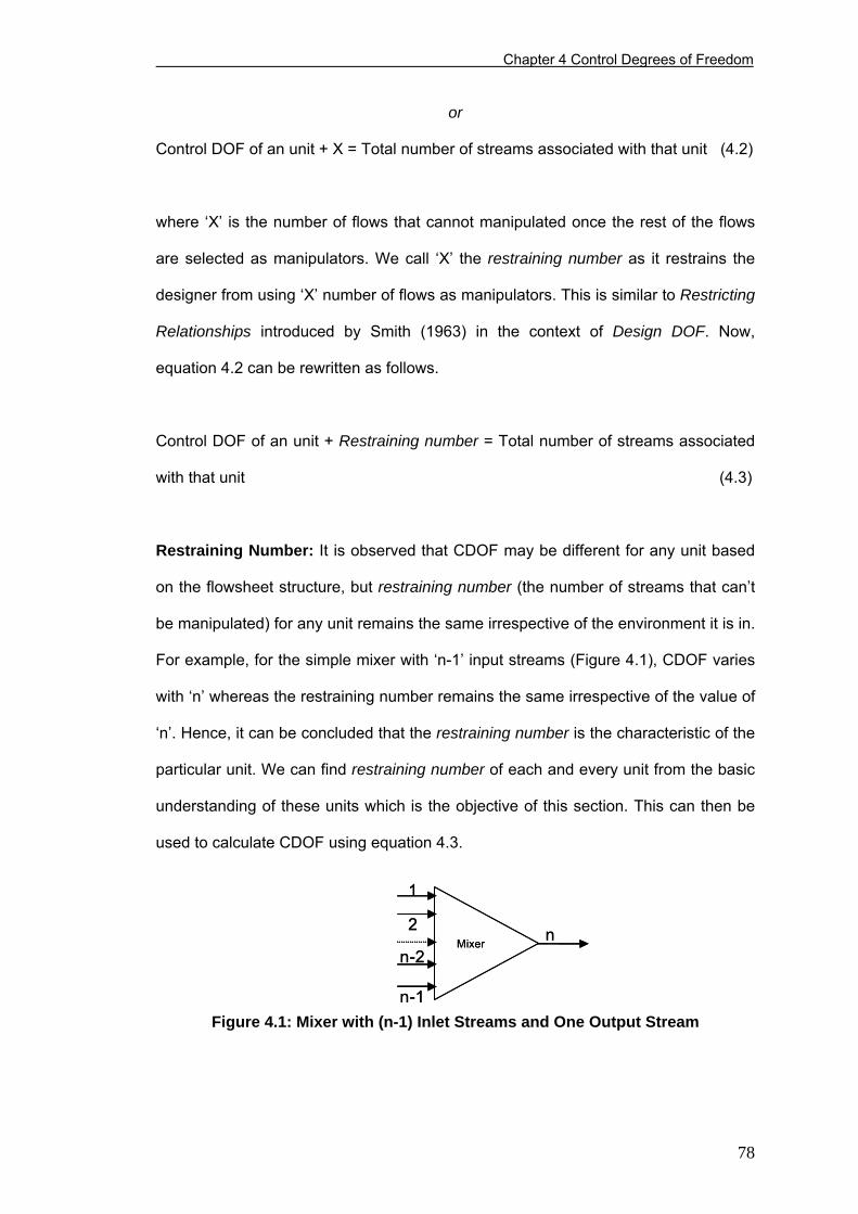
Chapter 4 Control Degrees of Freedom
or
Control DOF of an unit + X = Total number of streams associated with that unit (4.2)
where ‘X’ is the number of flows that cannot manipulated once the rest of the flows
are selected as manipulators. We call ‘X’ the restraining number as it restrains the
designer from using ‘X’ number of flows as manipulators. This is similar to Restricting
Relationships introduced by Smith (1963) in the context of Design DOF. Now,
equation 4.2 can be rewritten as follows.
Control DOF of an unit + Restraining number = Total number of streams associated
with that unit (4.3)
Restraining Number: It is observed that CDOF may be different for any unit based
on the flowsheet structure, but restraining number (the number of streams that can’t
be manipulated) for any unit remains the same irrespective of the environment it is in.
For example, for the simple mixer with ‘n-1’ input streams (Figure 4.1), CDOF varies
with ‘n’ whereas the restraining number remains the same irrespective of the value of
‘n’. Hence, it can be concluded that the restraining number is the characteristic of the
particular unit. We can find restraining number of each and every unit from the basic
understanding of these units which is the objective of this section. This can then be
used to calculate CDOF using equation 4.3.
Mixer
1
2 nn-2
n-1
Mixer
1
2 nn-2
n-1Figure 4.1: Mixer with (n-1) Inlet Streams and One Output Stream
78
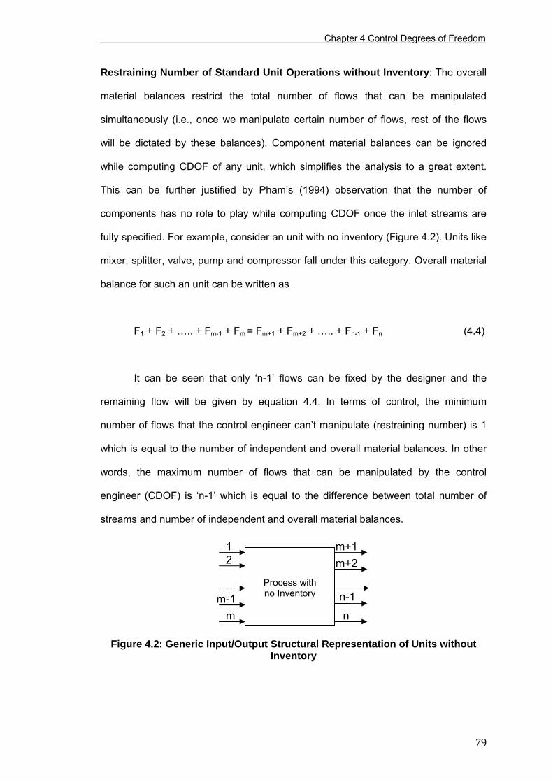
Chapter 4 Control Degrees of Freedom
Restraining Number of Standard Unit Operations without Inventory: The overall
material balances restrict the total number of flows that can be manipulated
simultaneously (i.e., once we manipulate certain number of flows, rest of the flows
will be dictated by these balances). Component material balances can be ignored
while computing CDOF of any unit, which simplifies the analysis to a great extent.
This can be further justified by Pham’s (1994) observation that the number of
components has no role to play while computing CDOF once the inlet streams are
fully specified. For example, consider an unit with no inventory (Figure 4.2). Units like
mixer, splitter, valve, pump and compressor fall under this category. Overall material
balance for such an unit can be written as
F1 + F2 + ….. + Fm-1 + Fm = Fm+1 + Fm+2 + ….. + Fn-1 + Fn (4.4)
It can be seen that only ‘n-1’ flows can be fixed by the designer and the
remaining flow will be given by equation 4.4. In terms of control, the minimum
number of flows that the control engineer can’t manipulate (restraining number) is 1
which is equal to the number of independent and overall material balances. In other
words, the maximum number of flows that can be manipulated by the control
engineer (CDOF) is ‘n-1’ which is equal to the difference between total number of
streams and number of independent and overall material balances.
Process with no Inventory
1 2
m-1 m
m+1
n-1
n
m+2
Figure 4.2: Generic Input/Output Structural Representation of Units without Inventory
79
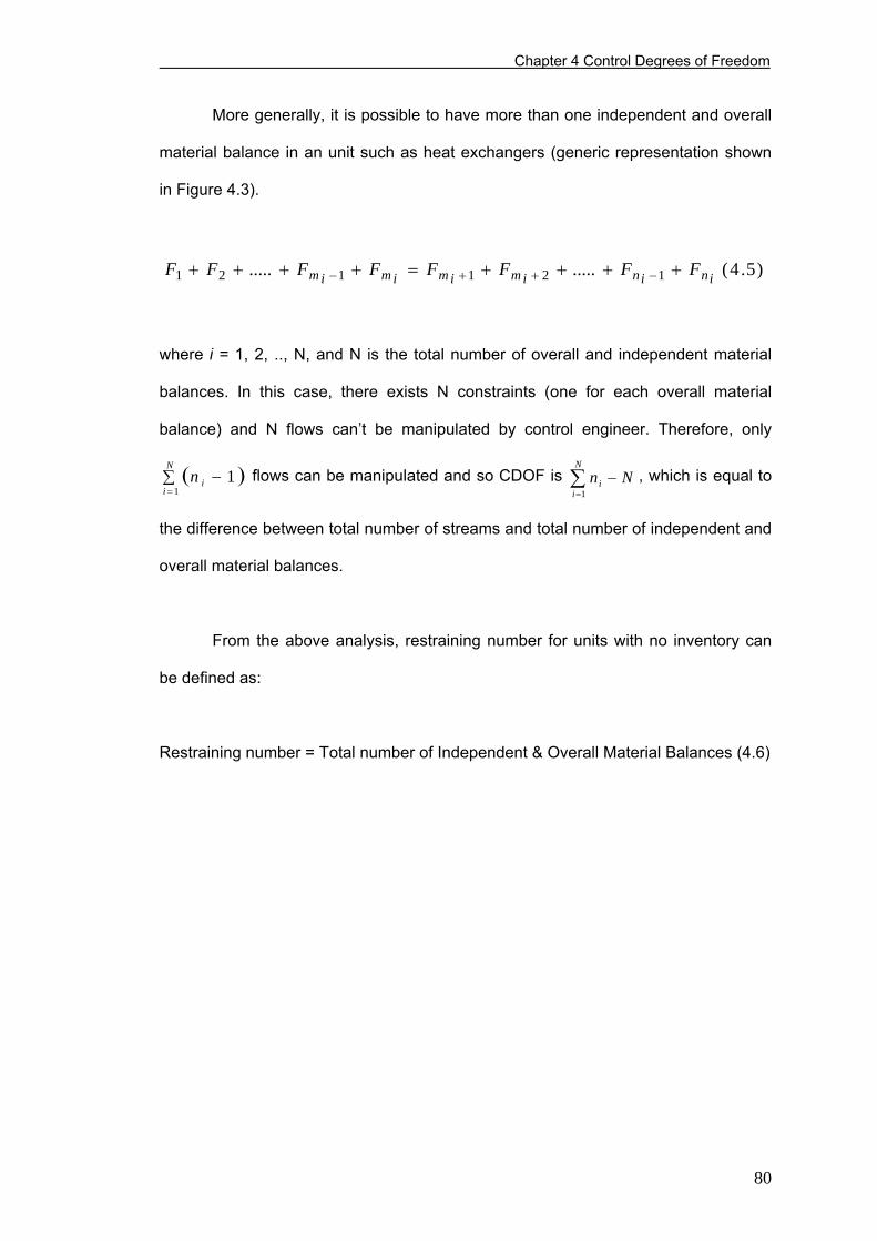
Chapter 4 Control Degrees of Freedom
More generally, it is possible to have more than one independent and overall
material balance in an unit such as heat exchangers (generic representation shown
in Figure 4.3).
)5.4(.......... 121121 ininimimimim FFFFFFFF ++++=++++ −++−
where i = 1, 2, .., N, and N is the total number of overall and independent material
balances. In this case, there exists N constraints (one for each overall material
balance) and N flows can’t be manipulated by control engineer. Therefore, only
flows can be manipulated and so CDOF is , which is equal to
the difference between total number of streams and total number of independent and
overall material balances.
(∑ −=
N
iin
11 ) Nn
N
ii −∑
=1
From the above analysis, restraining number for units with no inventory can
be defined as:
Restraining number = Total number of Independent & Overall Material Balances (4.6)
80
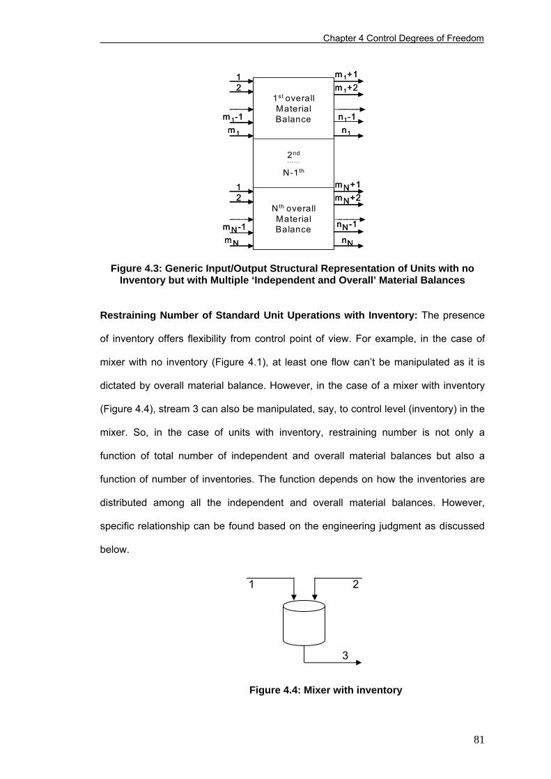
Chapter 4 Control Degrees of Freedom
m 1+1m 1+2
mN+1
2nd……
N-1th
1st overallMaterial Balance
12
m 1-1m 1
n1-1n1
Nth overallMaterial Balance
12
mN-1mN
nN-1
nN
mN+2
m 1+1m 1+2
mN+1
2nd……
N-1th
1st overallMaterial Balance
12
m 1-1m 1
n1-1n1
Nth overallMaterial Balance
12
mN-1mN
nN-1
nN
mN+2
Figure 4.3: Generic Input/Output Structural Representation of Units with no
Inventory but with Multiple ‘Independent and Overall’ Material Balances
Restraining Number of Standard Unit Uperations with Inventory: The presence
of inventory offers flexibility from control point of view. For example, in the case of
mixer with no inventory (Figure 4.1), at least one flow can’t be manipulated as it is
dictated by overall material balance. However, in the case of a mixer with inventory
(Figure 4.4), stream 3 can also be manipulated, say, to control level (inventory) in the
mixer. So, in the case of units with inventory, restraining number is not only a
function of total number of independent and overall material balances but also a
function of number of inventories. The function depends on how the inventories are
distributed among all the independent and overall material balances. However,
specific relationship can be found based on the engineering judgment as discussed
below.
1
3
2
Figure 4.4: Mixer with inventory
81
Chapter 4 Control Degrees of Freedom
In the case of units without inventory, it has been observed in the above
analysis that the overall material balance does not allow control engineer to
manipulate all the available process streams. However, in the case of units with
inventory, process variables associated with inventories (for example pressure for
vapor and level for liquid) offer additional flexibility from control point of view. If there
exists an inventory associated with an overall material balance, in principle, it is
possible to manipulate all the streams associated with that material balance either to
control the extensive or intensive variables as long as we don’t try to regulate all the
extensive variables or all the intensive variables simultaneously. Controlling all the
extensive variables violates overall mass balance (and leads to continuous
accumulation which is not desirable) if there is any disturbance or error in
measurements. Similarly, for any non-reactive system with fixed inlet composition,
according to Duhem’s theorem, specifying any two intensive variables completely
specifies the system and so it is not possible to control all the intensive variables
independently as they are dependant on one another.
For example, it can be seen from Figure 4.4 that the presence of inventory
allows us to manipulate all the streams associated with it to control 2 extensive
variables (say, flow rate of streams 1 and 2) and to control level (say, using stream 3
flow rate). Based on this, restraining number for units with inventories is given by
Restraining number = Total number of independent & overall material balances with
no associated inventory (4.7)
Equation 4.7 reduces to equation 4.6 in case of no inventory, and is generic
taking care of number of phases implicitly. Qualitative justification for this can be
given: any additional phase, which in turn creates additional inventory, in the unit will
82
Chapter 4 Control Degrees of Freedom
automatically be associated with an outlet stream. Based on the discussion given
above, this outlet stream can also be manipulated as it is associated with an
inventory. As an example, consider a flash separator whose restraining number is
zero as there are zero material balances with no inventory, irrespective of whether it
is two- or three-phase separator (i.e., all the flows can be manipulated, which is true).
All the standard units fall under two categories: units with overall material balances
with associated inventory or without associated inventory. Then, CDOF of an unit can
be calculated from equation 3 which is rewritten as:
Control DOF of an unit = Total number of streams associated with that unit –
Restraining number of that unit (4.8)
Table 4.1 gives the restraining number (from equation 4.7) and CDOF (from
equation 4.8) for several standard units. For other operations and/or situations, which
are not covered in Table 4.1, equation 4.8 can be used to obtain the corresponding
CDOF. In this table and subsequent figures, thick and thin lines represent energy and
material streams respectively.
The power of the proposed method can be seen when it is applied to
relatively complex and highly integrated processes. For such a process, CDOF is
given by
Control DOF for a process = Total number of streams in that process – Sum of the
restraining numbers for all the units in that process (4.9)
This is proved by considering a few simple and yet typical processes.
83
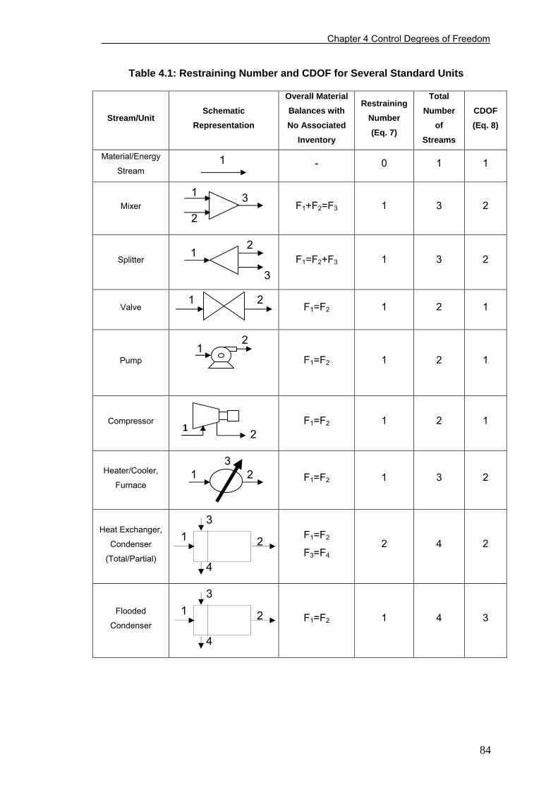
Chapter 4 Control Degrees of Freedom
Table 4.1: Restraining Number and CDOF for Several Standard Units
Stream/Unit Schematic
Representation
Overall Material Balances with No Associated
Inventory
Restraining Number (Eq. 7)
Total Number
of Streams
CDOF (Eq. 8)
Material/Energy
Stream - 0 1 1
Mixer
F1+F2=F3 1 3 2
Splitter
F1=F2+F3 1 3 2
1
1
2
3
21
3
Valve
F1=F2 1 2 1
Pump
F1=F2 1 2 1
Compressor
F1=F2 1 2 1
Heater/Cooler,
Furnace
F1=F2 1 3 2
Heat Exchanger,
(
2 4 2 Condenser
Total/Partial)
F1=F2
F3=F4
Flooded
CF1=F2 1 4 3
ondenser 2
3
4
1
1 2
2 1
1 2
1 2 3
2
3
4
1
84
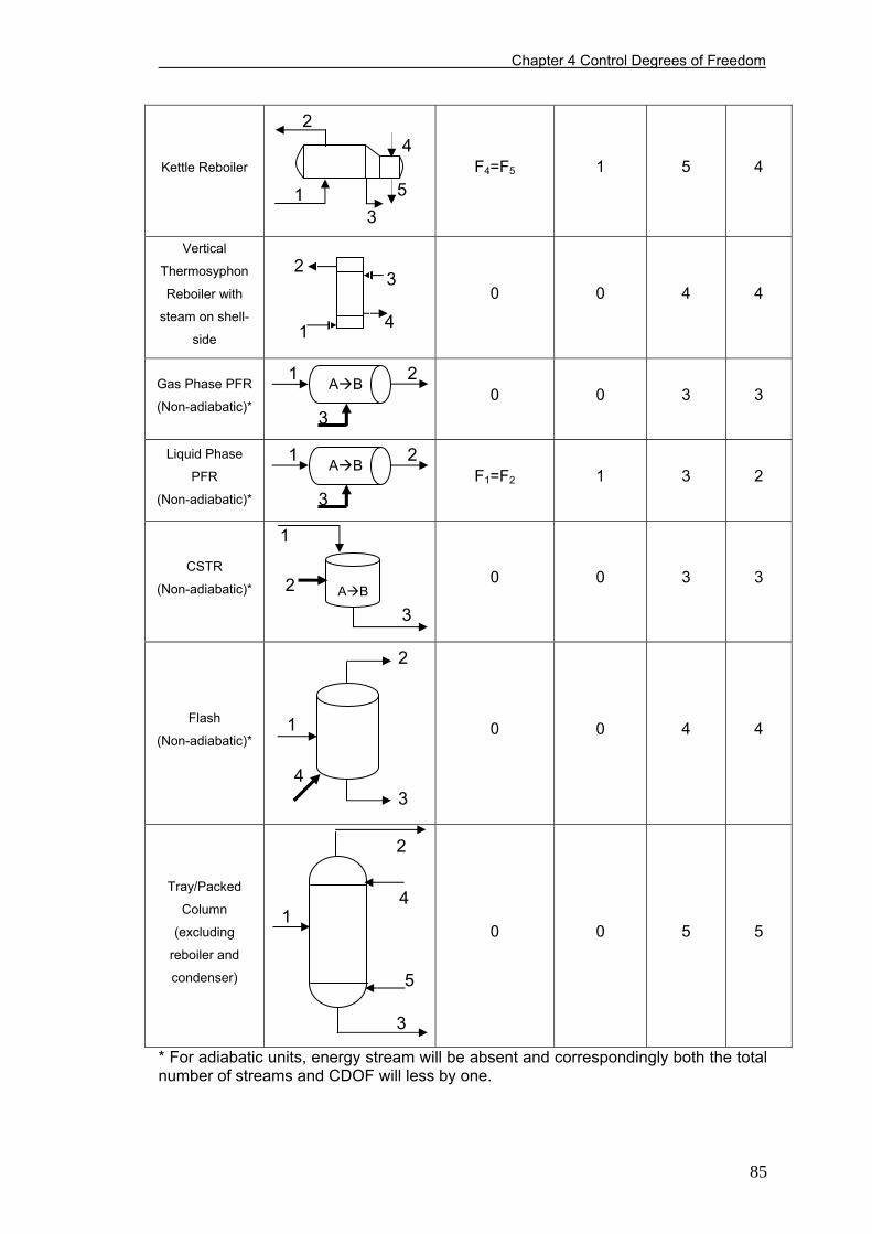
Chapter 4 Control Degrees of Freedom
Kettle Reboiler
F4=F5 1 5 4
Vertical
Thermosyphon
Reboiler with
steam on shell-
side
0 0 4 4
Gas Phase PFR
(Non-adiabatic)* 0 0 3 3
Liquid Phase
PFR
(Non-adiabatic)*
F1=F2 1 3 2
CSTR
(Non-adiabatic)* 0 0 3 3
Flash
(Non-adiabatic)*
0 0 4 4
Tray/Packed
Column
cluding
iler and
condenser)
4 2
1 5
2
1
3
4
3
A B 1 2
3
A B 1 2
3
A B
1
3
2
1
3
2
4
(ex
rebo
0 0 5 5 1
3
2
5
4
* For adiabatic units, energy stream will be absent and correspondingly both the total number of streams and CDOF will less by one.
85
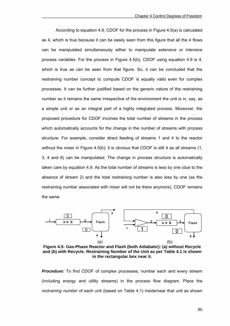
Chapter 4 Control Degrees of Freedom
According to equation 4.9, CDOF for the process in Figure 4.5(a) is calculated
as 4, which is true because it can be easily seen from this figure that all the 4 flows
can be manipulated simultaneously either to manipulate extensive or intensive
process variables. For the process in Figure 4.5(b), CDOF using equation 4.9 is 4,
which is true as can be seen from that figure. So, it can be concluded that the
restraining number concept to compute CDOF is equally valid even for complex
processes. It can be further justified based on the generic nature of the restraining
number as it remains the same irrespective of the environment the unit is in, say, as
a simple unit or as an integral part of a highly integrated process. Moreover, the
proposed procedure for CDOF involves the total number of streams in the process
which automatically accounts for the change in the number of streams with process
structure. For example, consider direct feeding of streams 1 and 4 to the reactor
without the mixer in Figure 4.5(b); it is obvious that CDOF is still 4 as all streams (1,
3, 4 and 6) can be manipulated. The change in process structure is automatically
taken care by equation 4.9. As the total number of streams is less by one (due to the
absence of stream 2) and the total restraining number is also less by one (as the
restraining number associated with mixer will not be there anymore), CDOF remains
the same.
A B F lash32
4
1
5
0
1 0
A B Flash21
4
30
0
A B F lash32
4
1
5
0
1 0
A B Flash21
4
30
0
(a) (b) Figure 4.5: Gas-Phase Reactor and Flash (both Adiabatic): (a) without Recycle and (b) with Recycle. Restraining Number of the Unit as per Table 4.1 is shown
in the rectangular box near it.
Procedure: To find CDOF of complex processes, number each and every stream
(including energy and utility streams) in the process flow diagram. Place the
restraining number of each unit (based on Table 4.1) inside/near that unit as shown
86
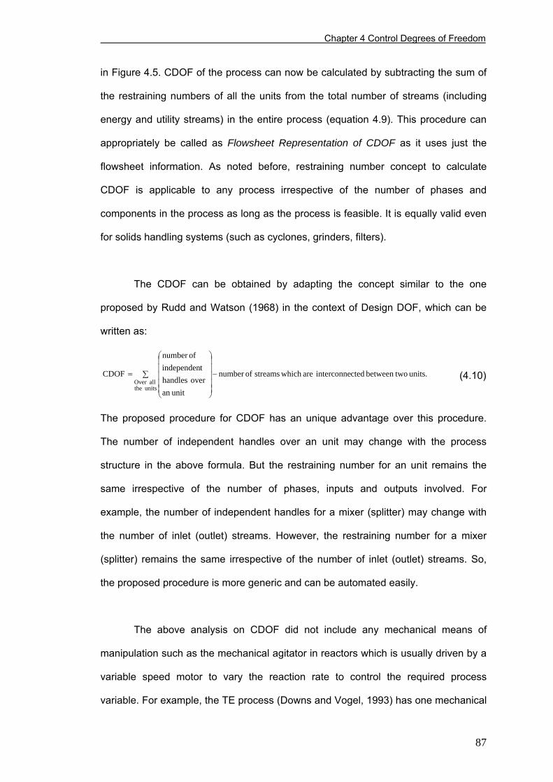
Chapter 4 Control Degrees of Freedom
in Figure 4.5. CDOF of the process can now be calculated by subtracting the sum of
the restraining numbers of all the units from the total number of streams (including
energy and utility streams) in the entire process (equation 4.9). This procedure can
appropriately be called as Flowsheet Representation of CDOF as it uses just the
flowsheet information. As noted before, restraining number concept to calculate
CDOF is applicable to any process irrespective of the number of phases and
components in the process as long as the process is feasible. It is equally valid even
for solids handling systems (such as cyclones, grinders, filters).
The CDOF can be obtained by adapting the concept similar to the one
proposed by Rudd and Watson (1968) in the context of Design DOF, which can be
written as:
units.twobetweenctedinterconnearewhichstreamsofnumber
unitanover handles
t independen ofnumber
CDOF
units the allOver
−∑
⎟⎟⎟⎟⎟
⎠
⎞
⎜⎜⎜⎜⎜
⎝
⎛
= (4.10)
The proposed procedure for CDOF has an unique advantage over this procedure.
The number of independent handles over an unit may change with the process
structure in the above formula. But the restraining number for an unit remains the
same irrespective of the number of phases, inputs and outputs involved. For
example, the number of independent handles for a mixer (splitter) may change with
the number of inlet (outlet) streams. However, the restraining number for a mixer
(splitter) remains the same irrespective of the number of inlet (outlet) streams. So,
the proposed procedure is more generic and can be automated easily.
The above analysis on CDOF did not include any mechanical means of
manipulation such as the mechanical agitator in reactors which is usually driven by a
variable speed motor to vary the reaction rate to control the required process
variable. For example, the TE process (Downs and Vogel, 1993) has one mechanical
87
Chapter 4 Control Degrees of Freedom
CDOF. So, CDOF should be increased by the corresponding number of mechanical
manipulators whenever available. In addition, it should be noted that the proposed
analysis for CDOF deals only with the process flows which can be manipulated
(using a control valve) simultaneously. The analysis has not considered any pressure
reduction valves which are used to set the pressure at a down-stream location.
However, pressure reduction valves can be placed on any pipeline as per process
requirements, even if the flow is being manipulated (because of the inherent
relationship between valve opening and pressure drop). Hence, the CDOF obtained
by the proposed procedure will increase by one for each pressure reduction valve
present in the process. Based on this, equation 4.9 can be updated as follows:
Control DOF for a process = Total number of streams in that process – Sum of the
restraining numbers for all the units in that process + The number of mechanical or
any other manipulators other than the process flows (such as agitators) and the
number of pressure reduction valves (i.e., the valves used exclusively for pressure
reduction) 4.11
It is important to note that CDOF gives the maximum number of flows that can
be manipulated simultaneously whereas the minimum number is dictated by stability
considerations. Actual number of manipulated variables (i.e., control valves) is
between the minimum number and CDOF. For example, minimum number of
manipulated variables for a distillation column (with condenser and reboiler) is 3 in
order to maintain its stable operation i.e., to control pressure, accumulator level and
level in the sump (in case of thermosyphon reboiler) or in kettle reboiler. On the other
hand, as discussed in the following section, CDOF for this column is 6. The additional
3 manipulated variables can be used for feed flow (which can be considered either as
a disturbance or as a manipulator), top and bottoms compositions. Based on the
process requirements, control engineer would go for single or double end
88
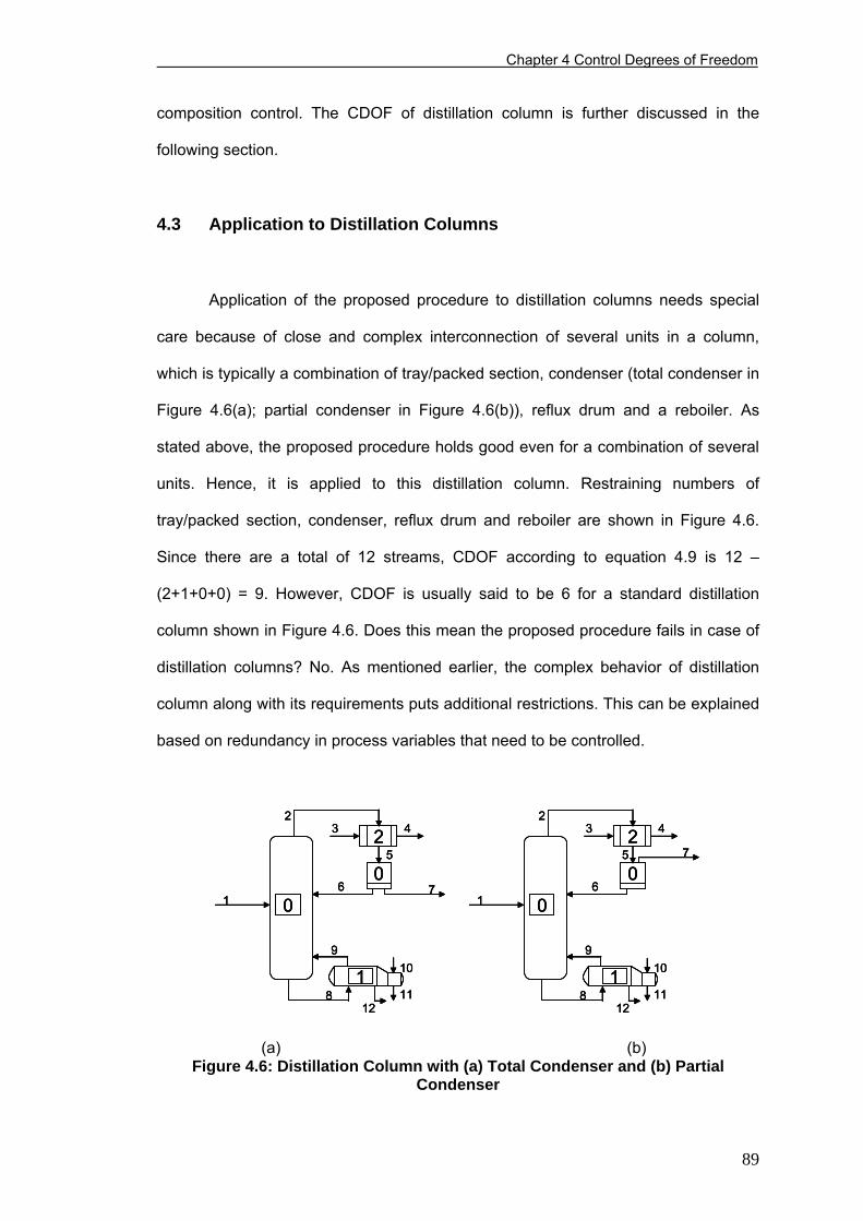
Chapter 4 Control Degrees of Freedom
composition control. The CDOF of distillation column is further discussed in the
following section.
4.3 Application to Distillation Columns
Application of the proposed procedure to distillation columns needs special
care because of close and complex interconnection of several units in a column,
which is typically a combination of tray/packed section, condenser (total condenser in
Figure 4.6(a); partial condenser in Figure 4.6(b)), reflux drum and a reboiler. As
stated above, the proposed procedure holds good even for a combination of several
units. Hence, it is applied to this distillation column. Restraining numbers of
tray/packed section, condenser, reflux drum and reboiler are shown in Figure 4.6.
Since there are a total of 12 streams, CDOF according to equation 4.9 is 12 –
(2+1+0+0) = 9. However, CDOF is usually said to be 6 for a standard distillation
column shown in Figure 4.6. Does this mean the proposed procedure fails in case of
distillation columns? No. As mentioned earlier, the complex behavior of distillation
column along with its requirements puts additional restrictions. This can be explained
based on redundancy in process variables that need to be controlled.
11
10
12
9
8
24
5
3
61
70
2
0
111
10
12
9
8
24
5
3
61
7
0
2
0
111
10
12
9
8
24
5
3
61
70
2
0
111
10
12
9
8
24
5
3
61
70
2
0
111
10
12
9
8
24
5
3
61
7
0
2
0
111
10
12
9
8
24
5
3
61
7
0
2
0
1
(a) (b) Figure 4.6: Distillation Column with (a) Total Condenser and (b) Partial
Condenser
89
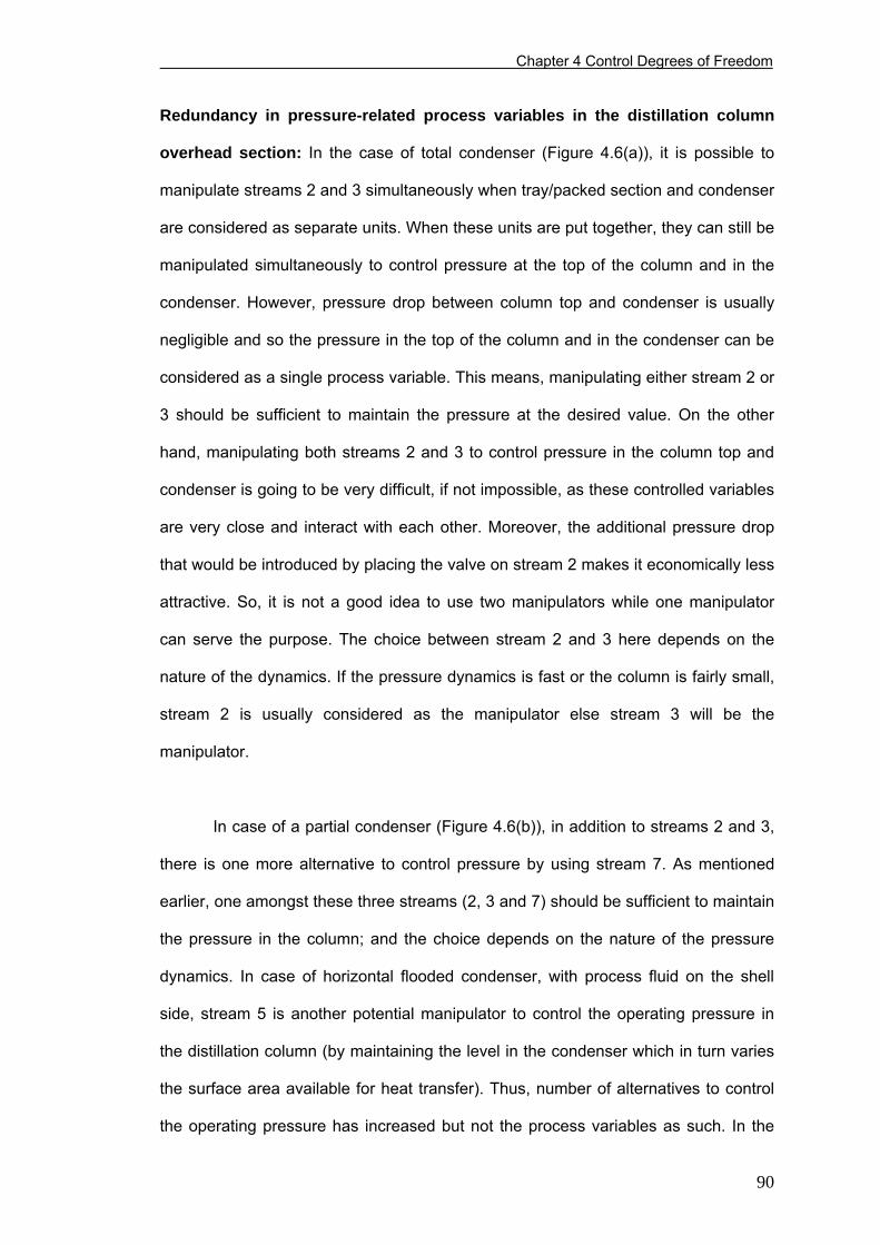
Chapter 4 Control Degrees of Freedom
Redundancy in pressure-related process variables in the distillation column
overhead section: In the case of total condenser (Figure 4.6(a)), it is possible to
manipulate streams 2 and 3 simultaneously when tray/packed section and condenser
are considered as separate units. When these units are put together, they can still be
manipulated simultaneously to control pressure at the top of the column and in the
condenser. However, pressure drop between column top and condenser is usually
negligible and so the pressure in the top of the column and in the condenser can be
considered as a single process variable. This means, manipulating either stream 2 or
3 should be sufficient to maintain the pressure at the desired value. On the other
hand, manipulating both streams 2 and 3 to control pressure in the column top and
condenser is going to be very difficult, if not impossible, as these controlled variables
are very close and interact with each other. Moreover, the additional pressure drop
that would be introduced by placing the valve on stream 2 makes it economically less
attractive. So, it is not a good idea to use two manipulators while one manipulator
can serve the purpose. The choice between stream 2 and 3 here depends on the
nature of the dynamics. If the pressure dynamics is fast or the column is fairly small,
stream 2 is usually considered as the manipulator else stream 3 will be the
manipulator.
In case of a partial condenser (Figure 4.6(b)), in addition to streams 2 and 3,
there is one more alternative to control pressure by using stream 7. As mentioned
earlier, one amongst these three streams (2, 3 and 7) should be sufficient to maintain
the pressure in the column; and the choice depends on the nature of the pressure
dynamics. In case of horizontal flooded condenser, with process fluid on the shell
side, stream 5 is another potential manipulator to control the operating pressure in
the distillation column (by maintaining the level in the condenser which in turn varies
the surface area available for heat transfer). Thus, number of alternatives to control
the operating pressure has increased but not the process variables as such. In the
90
Chapter 4 Control Degrees of Freedom
case of vertical flooded condenser where the process fluid is usually inside the tubes,
we can’t manipulate stream 5, but coolant flow (stream 3) can be manipulated to
maintain the coolant level on shell side to vary the heat transfer area which in turn
maintains the pressure.
Redundancy in level-related process variables in the distillation column with
kettle reboiler: The sump level and the reboiler level can be controlled if they are
considered as independent units. They can in principle be controlled simultaneously
even when they are put together. However, when they are considered together, the
sump level is redundant and need not be controlled explicitly because the
mechanical design ensures that the sump level is maintained all the time by virtue of
constant level (because of the baffle) in the reboiler. There are two fundamental
reasons which make the sump level self-regulating. If there is any disturbance and
the sump level is increasing, then (1) because of the increased static pressure the
flow will be more at the bottom of the column to the reboiler as it is based on natural
circulation where the flow is a function of static head and (2) because of the
increased static pressure the bubble point of the bottoms stream will rise and
vaporization will be less thus reducing the reboiler pressure which creates
hydrostatically unbalanced system momentarily. The cumulative effect of these two
factors forces the flow over the baffle more (in to surge) and boil-up rate less. Owing
to the latter, density of fluid on trays in the column will rise and overflow over the
weirs will be less which in turn decreases the sump level till it reaches the original
value, to return to the hydrostatic balance between the sump level and static head
held by baffle. There is a possibility of inverse response in the bottom sump level.
However, for the sake of simplicity in the analysis, this is not mentioned in the above
reasoning. The principle here is similar to the hydrostatic balance in an U tube except
that the analysis is more complex because of the interaction between material and
91
Chapter 4 Control Degrees of Freedom
energy. Similar reasoning can be given even if there is a disturbance which reduces
the sump level.
Based on the above discussion, the sump level is a redundant process
variable from control point of view as it is hydrostatically balanced because of the
static head held by baffle in the reboiler. Of course, the distillation bottom section and
reboiler should be properly designed else flooding can easily take place. For
example, mechanical design decisions such as the spacing between the sump level
and vapor entrance nozzle at the bottom of the column and the space above the
baffle in the kettle reboiler for liquid disengagement should be properly chosen to
easily resume hydrostatic balance in the system and to avoid flooding.
Redundancy in pressure-related process variables in the distillation column
with kettle reboiler: Pressure in a kettle reboiler can be a process variable when it is
alone (though it is not usual practice to control the pressure in the reboiler, it is
theoretically possible). Once it is part of a distillation column, pressure control at the
top of the column would ensure the pressure in the other parts and there is no need
to control the pressure in the reboiler. Hence, this is also a redundant pressure-
related process variable.
In view of above 3 redundant process variables, the effective CDOF is only 6
(= 9 - 3) which is usually the case. So, in the following cases, the restraining number
for a distillation column (with total/partial condenser and with kettle reboiler) is
increased by 3 to account for the 3 redundant process variables. In the case of
distillation columns with internal reboilers/open steam, the redundancy is only one
which is associated with the pressure-related process variables in the overhead as
there are no redundant process variables at the bottom of the column. Distillation
columns with thermosyphon reboiler of any configuration (vertical or horizontal; with
92
Chapter 4 Control Degrees of Freedom
or without baffle in the sump; Sloley, 1997) can be analyzed similar to that of the
distillation column with kettle reboiler to find the redundancy before applying the
concept of restraining number to compute the effective CDOF. For example, in the
most commonly used thermosyphon reboiler (i.e., vertical with steam on shell side),
the process stream that comes out of reboiler can, in principle, be manipulated to
control the pressure. However, as discussed in the case of kettle reboiler, it is not
required to control the pressure in the reboiler and hence this manipulated variable is
redundant. For complex distillation columns with additional side draws, which are
very common in petroleum refineries, each side draw increases the CDOF (by using
equation 4.9 and redundancy) by one and the proposed procedure will automatically
manifest this without any additional considerations.
4.4 Application to Complex Integrated Processes
In this section, the restraining number concept is applied to several highly
integrated processes of varying complexity to prove its applicability. The resulting
CDOFs are validated by comparing them with those available in the literature. For the
process in Figure 4.7, CDOF (from equation 9 and the concept of redundancy) is 6 [=
Total number of streams – (Sum of restraining numbers of all units + Number of
redundant process variables associated with stripper) = 9 – (1+2)]. According to
Luyben (1996), CDOF is 4. However, he presumes constant temperature in the
reactor and constant pressure in the stripper which contribute two more variables to
CDOF. So, total CDOF is 6 which is the same as that obtained by the proposed
procedure. In subsequent applications (including those in the Appendix B) total
CDOF from Luyben (1996) is considered for comparison. From Table 4.2, it can be
seen that the proposed procedure is successful in predicting the CDOF of highly
integrated processes in Figures 4.8 and 4.9 correctly. All the reactors in Figure 4.8
93
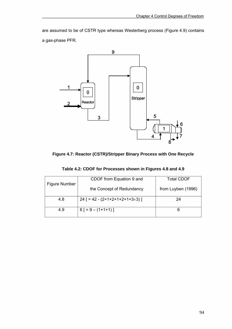
Chapter 4 Control Degrees of Freedom
are assumed to be of CSTR type whereas Westerberg process (Figure 4.9) contains
a gas-phase PFR.
7
6
8
5
4
ReactorStripper
9
3
1
2
00
17
6
8
5
4
ReactorStripper
9
3
1
2
00
1
Figure 4.7: Reactor (CSTR)/Stripper Binary Process with One Recycle
Table 4.2: CDOF for Processes shown in Figures 4.8 and 4.9
Figure Number CDOF from Equation 9 and
the Concept of Redundancy
Total CDOF
from Luyben (1996)
4.8 24 [ = 42 - (2+1+2+1+2+1+3×3) ] 24
4.9 6 [ = 9 – (1+1+1) ] 6
94
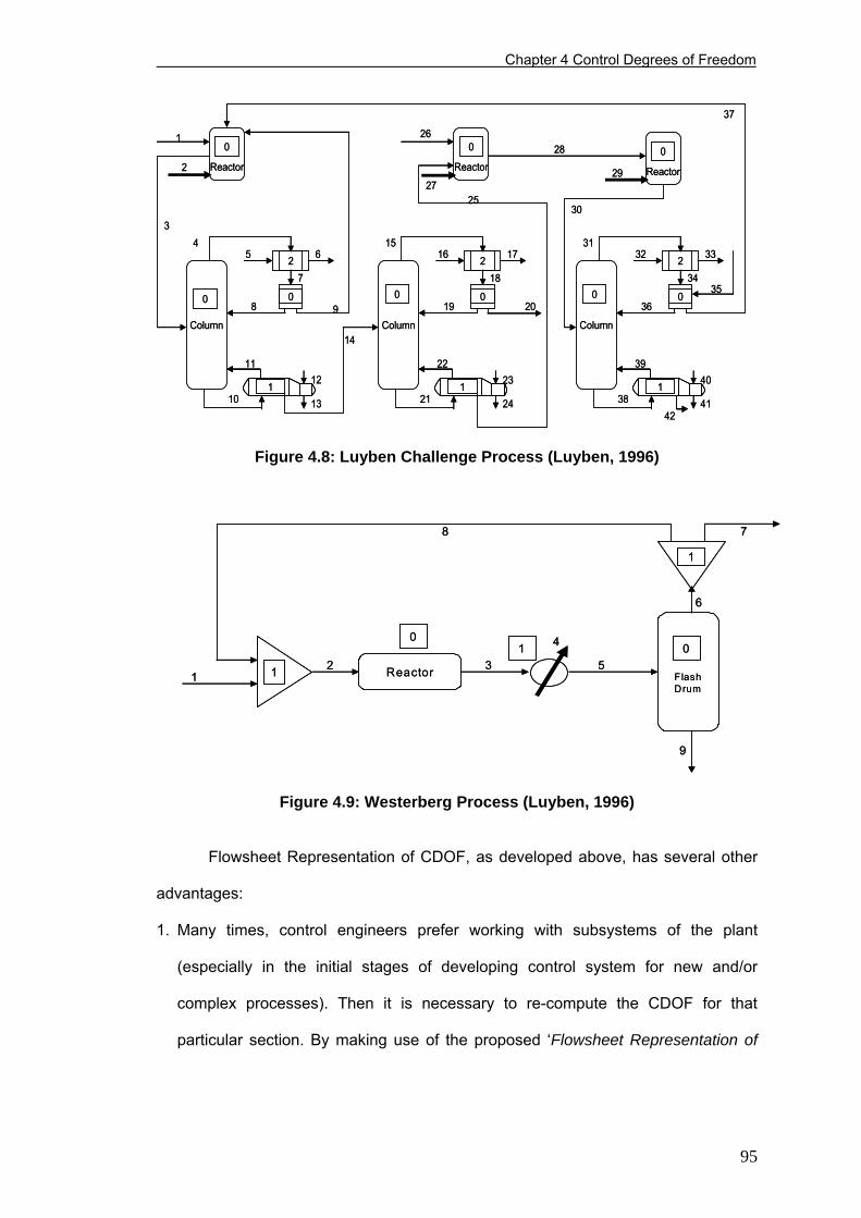
Chapter 4 Control Degrees of Freedom
27
24
23
25
22
21
Reactor
Column
15
37
1
2
17
18
16
19
41
40
42
39
38
Column
3133
34
32
3620
13
12
14
11
10
Column
46
7
5
8 9
Reactor
26
Reactor
30
29
3
28
35
000
000
2 2 2
00 0
1 1 1
27
24
23
25
22
21
Reactor
Column
15
37
1
2
17
18
16
19
41
40
42
39
38
Column
3133
34
32
3620
13
12
14
11
10
Column
46
7
5
8 9
Reactor
26
Reactor
30
29
3
28
35
000
000
2 2 2
00 0
1 1 1
Figure 4.8: Luyben Challenge Process (Luyben, 1996)
Reactor FlashDrum
3 5
4
2
8
1
9
7
6
10
1
1
0
Reactor FlashDrum
3 5
4
2
8
1
9
7
6
10
1
1
0
Figure 4.9: Westerberg Process (Luyben, 1996)
Flowsheet Representation of CDOF, as developed above, has several other
advantages:
1. Many times, control engineers prefer working with subsystems of the plant
(especially in the initial stages of developing control system for new and/or
complex processes). Then it is necessary to re-compute the CDOF for that
particular section. By making use of the proposed ‘Flowsheet Representation of
95
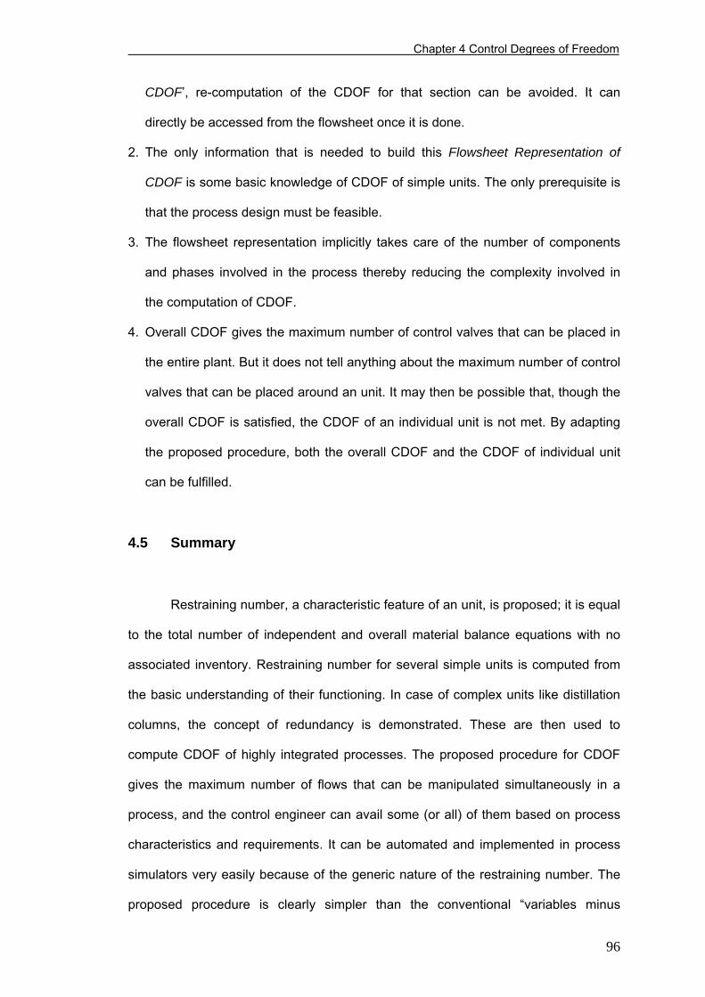
Chapter 4 Control Degrees of Freedom
CDOF’, re-computation of the CDOF for that section can be avoided. It can
directly be accessed from the flowsheet once it is done.
2. The only information that is needed to build this Flowsheet Representation of
CDOF is some basic knowledge of CDOF of simple units. The only prerequisite is
that the process design must be feasible.
3. The flowsheet representation implicitly takes care of the number of components
and phases involved in the process thereby reducing the complexity involved in
the computation of CDOF.
4. Overall CDOF gives the maximum number of control valves that can be placed in
the entire plant. But it does not tell anything about the maximum number of control
valves that can be placed around an unit. It may then be possible that, though the
overall CDOF is satisfied, the CDOF of an individual unit is not met. By adapting
the proposed procedure, both the overall CDOF and the CDOF of individual unit
can be fulfilled.
4.5 Summary
Restraining number, a characteristic feature of an unit, is proposed; it is equal
to the total number of independent and overall material balance equations with no
associated inventory. Restraining number for several simple units is computed from
the basic understanding of their functioning. In case of complex units like distillation
columns, the concept of redundancy is demonstrated. These are then used to
compute CDOF of highly integrated processes. The proposed procedure for CDOF
gives the maximum number of flows that can be manipulated simultaneously in a
process, and the control engineer can avail some (or all) of them based on process
characteristics and requirements. It can be automated and implemented in process
simulators very easily because of the generic nature of the restraining number. The
proposed procedure is clearly simpler than the conventional “variables minus
96

Chapter 4 Control Degrees of Freedom
equations” approach as it just needs fundamental understanding of simple units even
for highly integrated processes.
97
Chapter 5 Performance Assessment of PWC Systems
CHAPTER 5
PERFORMANCE ASSESSMENT OF PLANT-WIDE CONTROL
SYSTEMS*
Performance assessment of control systems has been receiving growing
attention in the recent past to improve operability and profit margins of the process.
However, such studies, and also the tools available to carry out such studies, from
plant-wide perspective are rather limited. In this regard, a new dynamic performance
index called DDS is proposed in this chapter. It is then used to assess the
performance of three PWC structures (CS1, CS2 and CS3) for the HDA process. The
three control structures are distinctly different from the TPM standpoint: CS1 uses
internal manipulator (e.g., reactor temperature), CS2 uses fixed-feed control strategy
with balanced nature, and CS3 uses on-demand control strategy to control the
throughput; consequently, rest of the control structure decisions are significantly
different. By critically analyzing the results from rigorous nonlinear dynamic
simulations, CS3 is observed to be exhibiting poorest overall dynamic performance.
The plant-wide dynamic performance of CS2 is found to be superior or comparable to
that of CS1 for all the anticipated disturbances. The analysis of the results reveals
the effectiveness of DDS and rigorous simulation tools for PWC studies.
5.1 Introduction
Performance assessment of control systems has been an active research
area for the last 15 – 20 years. Such studies from plant-wide perspective, however,
are relatively limited mainly due to the complexity involved in PWC due to the
* This chapter is based on the paper - Konda, N. V. S. N. M.; Rangaiah, G. P. Performance Assessment of Plant-Wide Control Systems of Industrial Processes. Ind. Eng. Chem. Res., 46, pp. 1220-1231. 2007.
98
Chapter 5 Performance Assessment of PWC Systems
presence of dozens of process variables; to complicate the matter further, recycles,
that are becoming common in chemical processes, are notorious for furthering
process complexity by increasing not only the interactions among process variables
but also process nonlinearity. Besides, the use of rigorous process simulators for
PWC studies is even more limited as it is more tedious and computationally intensive
to carry out such rigorous studies. In addition, performance assessment metrics
which can easily and effectively be used in PWC studies based on rigorous process
simulators are not available. Thus, in the present study, we propose a performance
metric and then use it to evaluate three PWC systems for the HDA process.
Due to the large number of process variables in any PWC problem, there
exists numerous alternative control structures. Controllability measures such as
RGA, NI, CN, DCN, RDG, PRG, and CLDG have been very useful to screen off
some control structures especially during the initial stages of control system design.
However, after the initial screening, a handful of alternatives will be left which needs
more rigorous analysis for the final selection. This can be done by simplified/linear
dynamic simulation as commonly done by most of the researchers in the past;
though, some researchers (e.g., Luyben, 2002) have been using rigorous nonlinear
dynamic simulators for some years.. However, due to the increasing use of recycles
in the chemical process industry, the processes are becoming more complex and
their dynamics can be highly nonlinear (Kumar and Daoutidis, 2002). Consequently,
there is a need to use rigorous nonlinear dynamic simulation, especially in the final
stages of control system design, to make the analysis more realistic (Kim et al.,
2000). In addition, some of the aforementioned metrics may not always yield reliable
results; He and Cai (2004) presented several case studies in which control
configuration design based on RGA and NI has failed. Similarly, Georgakis et al.
(2003) presented an operability measure which is more consistent than the metrics
such as RGA and CN.
99
Chapter 5 Performance Assessment of PWC Systems
At times, some of the above mentioned controllability measures cannot be
used due to the complexity of the process at hand. Noting this, Yi and Luyben (1995)
proposed a metric called steady-state disturbance sensitivity (SDS) based on steady-
state to screen the control structures; the basic idea here is to compute the changes
in the MV in the presence of disturbance(s) for different control structures. The
control structure that requires larger changes in MVs is not recommended as it is
more prone to hit constraints and valve-saturation limits. However, this measure
cannot be always used: consider two control structures, C1 and C2. If the required
changes in all the MVs in C1 are larger than that of C2, by making use of this
measure, the decision is obvious, i.e., C2 is better. However, if some MV changes in
C1 are less than that of C2 and the rest of the MV changes in C1 are more than that
of C2, the decision is less obvious. Besides, SDS does not consider the performance
during transient state and does not guarantee stability.
The use of any of the above tools is necessary but not sufficient, and should
subsequently be complemented with rigorous dynamic simulation. But, as mentioned
previously, in case of complex processes, such an analysis using nonlinear dynamic
simulations can be very difficult and computationally intensive due to the presence of
hundreds of control loops in a typical PWC system. Though, in principle, it is possible
to compare the performance of each individual loop, it is very tedious. At times, there
may not be any meaningful loop-to-loop comparison as a controlled variable in one
control structure need not necessarily be controlled in another control structure.
Alternatively, one might want to assign weights to each control loop to quantify the
overall performance into a single index. But, the weights are often subjective.
The rest of the chapter is organized as follows. The next section discusses
some of the common measures (in addition to the ones discussed above) and the
100
Chapter 5 Performance Assessment of PWC Systems
associated problems, and then presents the proposed metric to assess the
performance of PWC systems using rigorous simulation tools. Section 5.3 gives brief
overview of the HDA process and its steady-state simulation. Implementation of three
control structures for the HDA process in HYSYS is described in section 5.4. Their
performance is then critically analyzed (using rigorous nonlinear dynamic simulation)
in the presence of several anticipated disturbances in section 5.5. Finally, chapter
summary is given in section 5.6.
5.2 Plant-Wide Performance Assessment Measures
Elliott and Luyben (1995, 1996 & 1997) proposed capacity-based approach to
measure the dynamic performance of alternative control structures by computing the
loss in capacity due to off-spec production; the measure is thus related to product
quality regulation. Though capacity-based approach is a useful and practical
measure, it cannot be applied in all situations. For example, in this approach, the off-
spec product is assumed to be disposed. However, it may be economical to recycle it
as the raw materials are usually expensive. Otherwise, yield-losses and additional
costs due to disposal of the off-spec product may render the process uneconomical.
Though it is possible to implement this feature in the capacity-based approach, it
cannot be generalized. For example, it may not be desirable to recycle the over-
purified off-spec product (although the under-purified off-spec product needs to be
recycled) as it unnecessarily incurs additional costs. Even if the off-spec product has
to be recycled, the recycling location and reprocessing costs will be process-specific.
If the off-spec product is due to light impurities, it has to be recycled back to the light-
component (impurity) purification section else it has to be processed through the
heavy-component (impurity) purification section. At times, the off-spec product
cannot be recycled due to capacity limitations (Zheng and Mahajanam, 1999;
101
Chapter 5 Performance Assessment of PWC Systems
Mahajanam and Zheng, 2002) but has to be stored (for future processing) which
incurs additional inventory costs. Thus, reprocessing cost of the off-spec product will
be different in each of these cases, and no generally accepted procedures are
available to estimate it. One can assume some cost, but the results will be dependent
on this assumed value.
Product quality is important, but it cannot be the sole measure. For example,
using capacity-based approach and product quality as the measure, two alternative
designs will be dynamically equally good if both are capable of producing on-spec
product. However, this need not necessarily be true always. Consider product quality
regulation in case of alternatives CS2 and CS3 (yet to be discussed in sections 5.4
and 5.5); there is essentially no difference in this regulation of product quality in the
presence of uncertainty in the reaction kinetics (Figure 5.1, left). However, the same
disturbance has significantly different impact on dynamics of the two alternatives
(Figure 5.1, right). Hence, product quality regulation is only a necessary condition but
not sufficient to be considered as an overall process performance measure. Similar
example is presented in Chapter 6 (Section 6.3.1) to show the inadequacy of product
quality as the overall performance measure. In addition, the ultimate decision on
relative performance is likely to be biased on the performance of the product quality
loop (i.e., its manipulator and tuning) if one uses capacity-based approach as the
overall performance measure. In a similar way, the production rate also cannot be an
appropriate measure for the overall performance. For example, on-demand control
has better product-regulation capability, but its dynamics in the other parts of the
plant are much slower and thus dynamic performance is not as good as a fixed-feed
control strategy (Luyben, 1999).
102
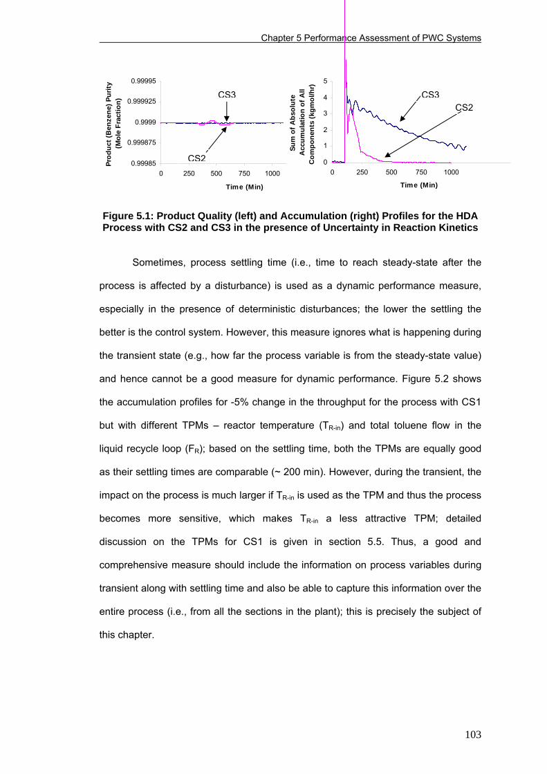
Chapter 5 Performance Assessment of PWC Systems
0.99985
0.999875
0.9999
0.999925
0.99995
0 250 500 750 1000
Time (Min)
Prod
uct (
Ben
zene
) Pur
ity
(Mol
e Fr
actio
n)
0
1
2
3
4
5
0 250 500 750 1000
Time (Min)
Sum
of A
bsol
ute
Acc
umul
atio
n of
All
Com
pone
nts
(kgm
ol/h
r)
CS3 CS2
CS3
CS2
Figure 5.1: Product Quality (left) and Accumulation (right) Profiles for the HDA Process with CS2 and CS3 in the presence of Uncertainty in Reaction Kinetics
Sometimes, process settling time (i.e., time to reach steady-state after the
process is affected by a disturbance) is used as a dynamic performance measure,
especially in the presence of deterministic disturbances; the lower the settling the
better is the control system. However, this measure ignores what is happening during
the transient state (e.g., how far the process variable is from the steady-state value)
and hence cannot be a good measure for dynamic performance. Figure 5.2 shows
the accumulation profiles for -5% change in the throughput for the process with CS1
but with different TPMs – reactor temperature (TR-in) and total toluene flow in the
liquid recycle loop (FR); based on the settling time, both the TPMs are equally good
as their settling times are comparable (~ 200 min). However, during the transient, the
impact on the process is much larger if TR-in is used as the TPM and thus the process
becomes more sensitive, which makes TR-in a less attractive TPM; detailed
discussion on the TPMs for CS1 is given in section 5.5. Thus, a good and
comprehensive measure should include the information on process variables during
transient along with settling time and also be able to capture this information over the
entire process (i.e., from all the sections in the plant); this is precisely the subject of
this chapter.
103
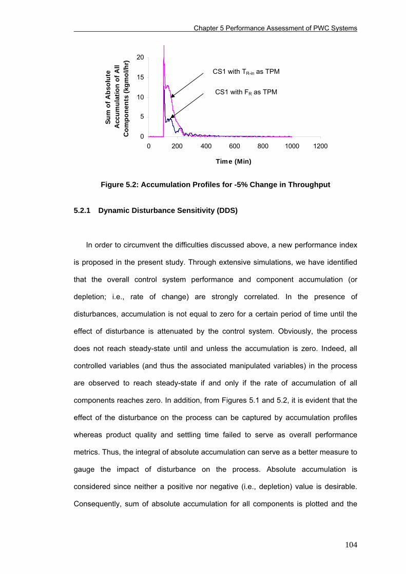
Chapter 5 Performance Assessment of PWC Systems
0
5
10
15
20
0 200 400 600 800 1000 1200
Time (Min)
Sum
of A
bsol
ute
Acc
umul
atio
n of
All
Com
pone
nts
(kgm
ol/h
r)
CS1 with TR-in as TPM
CS1 with FR as TPM
Figure 5.2: Accumulation Profiles for -5% Change in Throughput
5.2.1 Dynamic Disturbance Sensitivity (DDS)
In order to circumvent the difficulties discussed above, a new performance index
is proposed in the present study. Through extensive simulations, we have identified
that the overall control system performance and component accumulation (or
depletion; i.e., rate of change) are strongly correlated. In the presence of
disturbances, accumulation is not equal to zero for a certain period of time until the
effect of disturbance is attenuated by the control system. Obviously, the process
does not reach steady-state until and unless the accumulation is zero. Indeed, all
controlled variables (and thus the associated manipulated variables) in the process
are observed to reach steady-state if and only if the rate of accumulation of all
components reaches zero. In addition, from Figures 5.1 and 5.2, it is evident that the
effect of the disturbance on the process can be captured by accumulation profiles
whereas product quality and settling time failed to serve as overall performance
metrics. Thus, the integral of absolute accumulation can serve as a better measure to
gauge the impact of disturbance on the process. Absolute accumulation is
considered since neither a positive nor negative (i.e., depletion) value is desirable.
Consequently, sum of absolute accumulation for all components is plotted and the
104
Chapter 5 Performance Assessment of PWC Systems
area under the curve is used as a measure of PWC performance. Naturally, the
lesser the area, the better is the control and the corresponding alternative. As this
measure essentially quantifies the effect of disturbance on the process dynamics, it
will be referred as “Dynamic Disturbance Sensitivity (DDS)” and is defined as
( ) dticomponentofonaccumulatiabsoluteDDSst
t ntoi∫ ∑= = ⎟⎟
⎟
⎠
⎞
⎜⎜⎜
⎝
⎛=
0 1 (5.1)
where ts represents time taken to reach steady-state and n represents total number
of components involved in the process. Accumulation is computed using the standard
definition:
accumulation = input – output + generation – consumption (5.2)
where all the terms are based on ‘rate of change’. From the definition of DDS (i.e.,
sum of absolute errors in component material balances), it is similar to the other
metrics (such as Integral Absolute Error, i.e., IAE).
The proposed DDS has several advantages as discussed below:
1. It is easier to compute DDS for a process with relatively less number of
components than the number of loops, which often occurs; and data
management and storage will also be less demanding for calculating DDS for
such a process.
2. Procedure to compute DDS remains the same for a given process flow sheet
even if the control structure changes. This feature can be very handy for
analyzing performance of a large number of control structures and facilitates
easy automation of the procedure. The procedure can be further simplified by
ignoring some components present in insignificant quantities, as will be
shown in the Section 5.
105
Chapter 5 Performance Assessment of PWC Systems
3. Unlike any of the steady-state based counterparts, there exists strong
correlation between the value of DDS and process stability, as DDS is
computed based on dynamics; for an unstable system, DDS will be very
large.
4. DDS is more realistic as it considers level and pressure effects on dynamics
which have not been considered in the other measures based on steady-state
information.
5. In addition to screening alternative control structures, DDS can be used to
compare alternative process designs; this aspect is discussed in Chapter 6.
Furthermore, the relative impact of a disturbance on different sections of the
plant can be quantified using DDS.
6. It can be easily combined with rigorous nonlinear simulation models. This not
only improves the accuracy but also saves time as one does not have to
linearize the process models in order to make use of linear model-based
controllability indexes to analyze the performance.
7. DDS is equally applicable to performance analysis for set-point changes.
8. DDS is very useful to assess the dynamics of the process (such as overall
time constant) without having to examine all the process variables to identify
the slowest-responding one, which is dependent on several other factors
(e.g., type of disturbance).
9. Due to the fundamental nature of the DDS, it can be used even as an open-
loop controllability metric.
5.3 Process Description and Simulation of the HDA Process
For detailed information on the HDA process, refer to section 3.3.1 in Chapter
3. For a quicker and easier reference, process flow-sheet is given here (Figure 5.3)
106
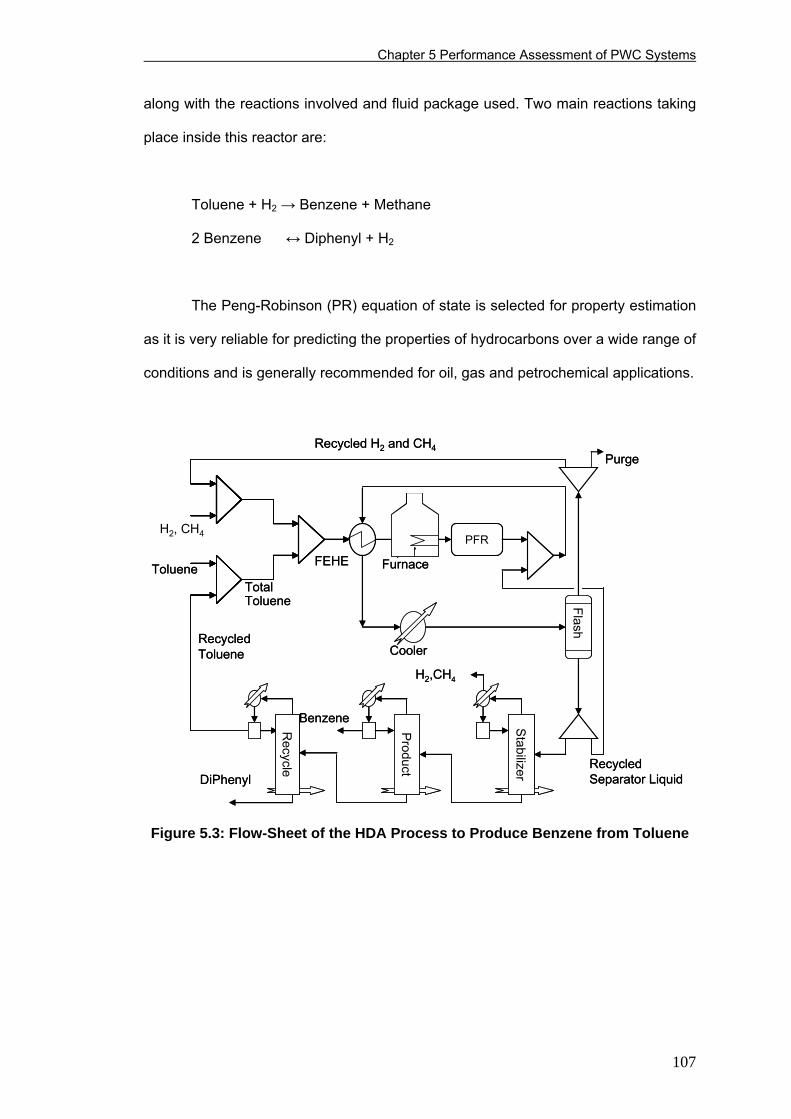
Chapter 5 Performance Assessment of PWC Systems
along with the reactions involved and fluid package used. Two main reactions taking
place inside this reactor are:
Toluene + H2 → Benzene + Methane
2 Benzene ↔ Diphenyl + H2
The Peng-Robinson (PR) equation of state is selected for property estimation
as it is very reliable for predicting the properties of hydrocarbons over a wide range of
conditions and is generally recommended for oil, gas and petrochemical applications.
Toluene
Purge
H2, CH4
Product
Stabilizer
PFR
Flash
FEHE Furnace
DiPhenyl
Benzene
H2,CH4
Cooler
Recycle
Recycled H2 and CH4
Recycled Toluene
Recycled Separator Liquid
Total Toluene
Toluene
Purge
H2, CH4
Product
Stabilizer
PFR
Flash
FEHE Furnace
DiPhenyl
Benzene
H2,CH4
Cooler
Recycle
Recycled H2 and CH4
Recycled Toluene
Recycled Separator Liquid
Total Toluene
Figure 5.3: Flow-Sheet of the HDA Process to Produce Benzene from Toluene
107
Chapter 5 Performance Assessment of PWC Systems
5.4 Dynamic Simulation of PWC Systems for the HDA Process
There has been increasing number of studies on PWC and several
methodologies have been proposed. However, there has not been any comparison of
these methods so-far. Thus, instead of randomly choosing the control structures, we
have chosen the candidate control structures resulting from different PWC methods.
Hence, the present study brings out the relative merits of different PWC
methodologies also. Several researchers have proposed different control structures
for the HDA process using their own methodologies. One of the popular PWC
methodologies is the heuristic procedure by Luyben and co-workers, and this method
was applied to the HDA process to develop PWC structure (Luyben et al., 1999). The
resulting control structure is considered in this study as one of the potential candidate
control structures and is referred to as CS1, hereafter. Two of the most recent
control structures for the HDA process, one by Konda et al. (2005) and the other by
Vasbinder et al. (2004), are also considered in this study for performance
assessment. Konda et al. (2005) proposed a PWC structure for the HDA process
based on an integrated framework consisting of improved heuristic method and
rigorous simulation tools. Vasbinder et al. (2004) proposed a PWC structure for the
HDA process using decision-based approach. The former is referred to as CS2 and
the latter as CS3 hereafter. Incidentally, these are the only three control structures
which have made use of rigorous dynamic simulation either in the control system
design stage (e.g., CS2) or in the validation stage of the resulting control system
(CS1 & CS3) for the detailed HDA process.
Other notable control structures for the HDA process are by Ponton and Laing
(1993) and Fonyo (1994). Konda et al. (2005) discussed the limitations of these
control structures; hence, these are not considered in the present study. Other
108
Chapter 5 Performance Assessment of PWC Systems
researchers have considered a simplified HDA process for control structure design
(e.g., Qiu et al., 2003) while others assumed some of the control decisions are
already in place (e.g., Jorgensen and Jorgensen, 2000; Herrmann et al., 2003); thus
the complete PWC structure for the entire HDA process cannot directly be extracted
from these works unless these methods are re-applied to develop complete PWC
system. Hence, these control structures could not be considered in this study.
5.4.1 Three Selected Control Structures (CS1, CS2, CS3)
CS1 is solely based on the heuristic procedure (Luyben et al., 1999). One of
the characteristic features of this heuristic procedure is to fix a flow in the recycle
loop to avoid the notorious effect of recycles - snowball effect. However, as observed
by other researchers, it is not always recommendable to fix the flow. For example,
Zheng et al. (1999) have studied several control structures (for a hypothetical
process) including the one with fixed-recycle-flow and observed that this control
structure is inferior to some other structures in which the recycle flow is not fixed.
CS2 is based on the integrated framework of heuristics and rigorous simulation
(Konda et al., 2005); in this framework, systematic analysis is carried out on recycles
while designing the control systems to minimize their impact on overall control
performance. CS3 is based on decision-based methodology (Vasbinder et al. 2004)
in which the modified analytical hierarchical process (mAHP) method is used to
decompose the HDA process into several modules and then Luyben’s heuristic
procedure is applied to each module to develop PWC system.
Interestingly, though each of these methods made use of Luyben’s heuristic
procedure in some form or other, the resulting control systems are significantly
different. Equally interesting is that these control structures can be classified into
three distinctly different categories based on the TPM: CS1 uses internal variable,
109
Chapter 5 Performance Assessment of PWC Systems
either reactor temperature, TR-in or total toluene flow, FR (i.e., sum of fresh toluene
and recycled toluene) - the present study considered both the alternatives; CS2 uses
process feed (i.e., fixed-feed control strategy); and CS3 uses production rate (i.e.,
on-demand control strategy) as the TPM. Consequently, rest of the control structure
of CS1, CS2 and CS3 are also very different, as shown in Table 5.1. CS1 and CS3
are shown in Table 5.1 after the implementation of the modifications discussed
below.
The only modification that is required for CS1 is replacing the cascade
controller for product purity (which manipulates the set point of temperature
controller) by a controller which directly manipulates reflux to regulate product purity.
This modification is observed to be necessary as the impact of the disturbance on the
process and settling time is found to be less after implementing this modification.
While this minor modification for CS1 is just to improve the dynamic performance,
CS3 required several changes mainly to stabilize the process and also to make it
more realistic. For example, Vasbinder et al. (2004) controlled H2 to toluene ratio
whereas the actual constraint for the HDA process is on the ratio between H2 and
aromatics (McKetta, 1977; Douglas, 1988). So, in the present study, H2 to aromatics
ratio controller is implemented.
With this H2 to aromatics ratio controller, we tried to implement CS3 as was
proposed by Vasbinder et al. (2004). However, the process was not stable and we
have identified that there was no controller which propagates the production rate
changes back to the upstream of stabilizer. Since there should be consistent back-
propagation of changes in any on-demand control strategy, we have considered the
stabilizer feed flow (instead of reboiler duty) as the manipulator to control stabilizer
reboiler level; note that the stabilizer feed flow was used to control flash level by
Vasbinder et al. (2004). The flash level is then controlled by toluene feed flow. With
110
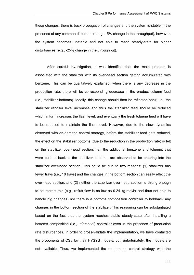
Chapter 5 Performance Assessment of PWC Systems
these changes, there is back propagation of changes and the system is stable in the
presence of any common disturbance (e.g., -5% change in the throughput), however,
the system becomes unstable and not able to reach steady-state for bigger
disturbances (e.g., -25% change in the throughput).
After careful investigation, it was identified that the main problem is
associated with the stabilizer with its over-head section getting accumulated with
benzene. This can be qualitatively explained: when there is any decrease in the
production rate, there will be corresponding decrease in the product column feed
(i.e., stabilizer bottoms). Ideally, this change should then be reflected back; i.e., the
stabilizer reboiler level increases and thus the stabilizer feed should be reduced
which in turn increases the flash level, and eventually the fresh toluene feed will have
to be reduced to maintain the flash level. However, due to the slow dynamics
observed with on-demand control strategy, before the stabilizer feed gets reduced,
the effect on the stabilizer bottoms (due to the reduction in the production rate) is felt
on the stabilizer over-head section; i.e., the additional benzene and toluene, that
were pushed back to the stabilizer bottoms, are observed to be entering into the
stabilizer over-head section. This could be due to two reasons: (1) stabilizer has
fewer trays (i.e., 10 trays) and the changes in the bottom section can easily effect the
over-head section; and (2) neither the stabilizer over-head section is strong enough
to counteract this (e.g., reflux flow is as low as 0.24 kg-mol/hr and thus not able to
handle big changes) nor there is a bottoms composition controller to holdback any
changes in the bottom section of the stabilizer. This reasoning can be substantiated
based on the fact that the system reaches stable steady-state after installing a
bottoms composition (i.e., inferential) controller even in the presence of production
rate disturbances. In order to cross-validate the implementation, we have contacted
the proponents of CS3 for their HYSYS models, but, unfortunately, the models are
not available. Thus, we implemented the on-demand control strategy with the
111
Chapter 5 Performance Assessment of PWC Systems
minimal modifications as discussed above. These changes are required in order to
establish a stable system which can handle some common disturbances. As will be
discussed in the later sections, CS3 failed to stabilize the process for six out of fifteen
disturbances studied; though the process can be stabilized for the rest of the
disturbances, the performance of CS3 is observed to be inferior to that of other
control structures.
5.4.2 Plant-Wide Controller Tuning
Controller tuning from plant-wide perspective is tedious due to the large of
number of controllers which are interacting with one another. In addition, one
particular set of tuning parameters for a control system does not necessarily work for
all disturbances as the impact of different disturbances on various sections of the
plant can be very different. For example, by using auto-tuning technique, a controller
gain of 2.3 is obtained for reactor outlet temperature controller (i.e., second controller
in Table 5.2) for CS2. Though this is acceptable for most of the disturbances, the
process becomes unstable for disturbances associated with uncertainty in kinetics.
The tuning parameters are observed to be more aggressive for this disturbance; ten-
folded reduction in the gain (i.e., a controller gain of 0.25) makes it stable for all types
of disturbances. This example shows how critical the tuning parameters of each
controller in the plant since inappropriate tuning parameters of single controller can
make the entire process unstable. So, extensive simulations are carried out in the
present study to make sure that the tuning parameters of all the controllers are robust
(to give stable response for most of the disturbances) as well as aggressive enough
(to give reasonably good performance). On the other hand, the same controller
(which required a gain of 0.25 in CS2, i.e., second controller in Table 5.2) can be
very aggressive with a gain of 1.32 in CS1 (i.e., five-times that of what is used in
CS2). This explains how dependent the tuning of each controller on the overall
112
Chapter 5 Performance Assessment of PWC Systems
control structure. Thus, it is important to consider the plant-wide perspective, not only
during structural decisions stage but also while tuning the controllers.
In general, all the controllers (except level controllers) are designed as PI-
controllers and P-only controllers are used for level control. Generic tuning
parameters are given for flow, level and pressure controllers in Luyben (2002), and
are used as initial estimates for these three types of controllers in all the control
structures. Wherever possible, for level and pressure controllers, aggressive tuning is
used (e.g., a gain of 10 for fifth controller in Table 5.2) and, if required, conservative
tuning is used (e.g., a gain of 2 for several level controllers in the separation section).
For temperature and composition controllers, initial estimates for tuning parameters
are obtained using auto-tuning technique. Understandably, auto-tuner gives
comparable tuning parameters with slight differences, if the control structure of any
controller remains the same in CS1, CS2 and CS3 (e.g., 1st, 3rd, 23rd, 24th, 28th and
30th controllers in Table 5.2). The slight differences are due to the different
interactions that these controllers encounter from other controllers in CS1, CS2 and
CS3. Understandably, auto-tuner gave entirely different tuning parameters if the
control structure of any controller is different in CS1, CS2 and CS3 (e.g., 8th controller
in Table 5.2). All these controllers are then fine tuned to give stable and reasonably
good performance in the presence of most of the anticipated disturbances. Final
tuning parameters for the controllers in the three control structures are given in Table
5.2.
113
Chapter 5 Performance Assessment of PWC Systems
Table 5.1: Details of Controlled and Manipulated Variables of CS1, CS2 and CS3
Manipulated Variable (MV) Controlled Variable (CV) CS1# CS2 CS3#
1. Cooler Tout Cooling Water Flow Cooling Water Flow Cooling Water Flow 2. Reactor Tout Quench Flow Rate Quench Flow Rate Quench Flow Rate 3. Reactor Tin Furnace Fuel - Furnace Fuel 4. Conversion - Furnace Fuel - 5. Flash Level Stabilizer Feed Stabilizer Feed Toluene Feed Flow
(Stabilizer Feed Flow)6. Flash Pressure - Flash Vapor Flow Flash Vapor Flow 7. Recycle Gas Pressure H2 Feed Flow - - 8. Purge Composition Purge Flow Compressor Duty - 9. Purge Flow - - Purge Flow 10. H2 to Aromatics Ratio - H2 Feed Flow H2 Feed Flow 11. Total Toluene Flow Total Toluene Flow - - 12. Toluene Feed - Toluene Feed Flow -
Stabilizer 13. Condenser Pressure Distillate Flow Distillate Flow Distillate Flow 14. Condenser Level Condenser Duty Condenser Duty Condenser Duty 15. Reboiler Level Bottoms Flow Bottoms Flow Stabilizer Feed Flow
(Reboiler Duty) 16. Distillate Composition - Reflux Flow Reflux Flow 17. Reflux Flow Reflux Flow - - 18. 7th Tray Temperature* Reboiler Duty Reboiler Duty Reboiler Duty
(no manipulator) Product (Benzene) Column
19. Condenser Pressure Condenser Duty Condenser Duty Condenser Duty 20. Condenser Level Distillate Flow Distillate Flow Product Column Feed 21. Reboiler Level Bottoms Flow Bottoms Flow Bottoms Flow 22. Product (Benzene) Flow
- - Distillate Flow
23. Distillate Composition Reflux Flow (set point of bottoms temperature controller)
Reflux Flow Reflux Flow
24. 40th Tray Temperature*
Reboiler Duty Reboiler Duty Reboiler Duty
Recycle (Toluene) Column 25. Condenser Pressure Condenser Duty Condenser Duty Condenser Duty 26. Condenser Level Toluene Feed Flow Distillate Flow Distillate Flow 27. Reboiler Level Reboiler Duty Reboiler Duty Bottoms Flow 28. Distillate Composition - Reflux Flow Reflux Flow 29. Reflux Flow Reflux Flow - - 30. Bottoms Composition - Bottoms Flow Reboiler Duty 31. 18th Tray Temperature*
Bottoms Flow - -
*Trays are counted from the top, with condenser as 0th tray. #CS1 and CS3 are shown in this table after the implementation of the modifications, as per the discussion in Section 5.4. Modified MVs are italicized and the original MVs are bracketed.
114
Chapter 5 Performance Assessment of PWC Systems
5.4.3 Disturbances Studied
It is very common to consider two or three types of disturbances while
assessing the performance of control systems. However, as will be discussed in
section 5.5, the control structure that works for a disturbance does not necessarily
work for other types of disturbances as the nature of each disturbance is unique.
Thus, there is a need to study several anticipated disturbances. Hence, in the
present study, 15 important and most common disturbances are studied (Table 5.3).
As there is a possibility of encountering more than one disturbance at a time, we
have considered dual disturbances as well. For example, the disturbances d8 to d11
are essentially the combinations of other disturbances (i.e., d1 and d2 with d4 and d5;
any other combination can also be considered). Similarly, uncertainties in reaction
kinetics are also simulated as disturbances. For convenience, a tag is assigned to
each disturbance; i.e., first disturbance will be referred to as d1, second one as d2 and
so on (see Table 5.3).
115
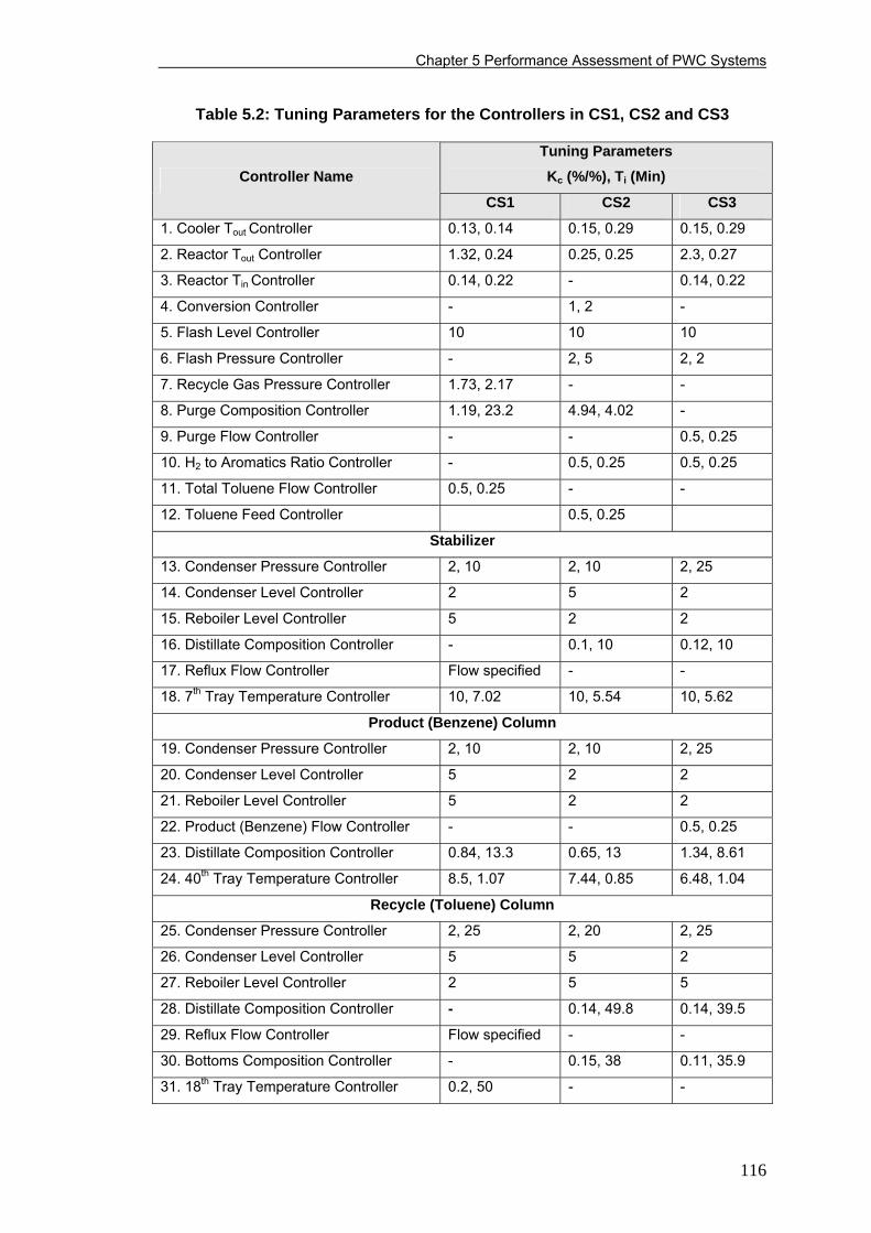
Chapter 5 Performance Assessment of PWC Systems
Table 5.2: Tuning Parameters for the Controllers in CS1, CS2 and CS3
Tuning Parameters Kc (%/%), Ti (Min) Controller Name
CS1 CS2 CS3
1. Cooler Tout Controller 0.13, 0.14 0.15, 0.29 0.15, 0.29
2. Reactor Tout Controller 1.32, 0.24 0.25, 0.25 2.3, 0.27
3. Reactor Tin Controller 0.14, 0.22 - 0.14, 0.22
4. Conversion Controller - 1, 2 -
5. Flash Level Controller 10 10 10
6. Flash Pressure Controller - 2, 5 2, 2
7. Recycle Gas Pressure Controller 1.73, 2.17 - -
8. Purge Composition Controller 1.19, 23.2 4.94, 4.02 -
9. Purge Flow Controller - - 0.5, 0.25
10. H2 to Aromatics Ratio Controller - 0.5, 0.25 0.5, 0.25
11. Total Toluene Flow Controller 0.5, 0.25 - -
12. Toluene Feed Controller 0.5, 0.25
Stabilizer
13. Condenser Pressure Controller 2, 10 2, 10 2, 25
14. Condenser Level Controller 2 5 2
15. Reboiler Level Controller 5 2 2
16. Distillate Composition Controller - 0.1, 10 0.12, 10
17. Reflux Flow Controller Flow specified - -
18. 7th Tray Temperature Controller 10, 7.02 10, 5.54 10, 5.62
Product (Benzene) Column
19. Condenser Pressure Controller 2, 10 2, 10 2, 25
20. Condenser Level Controller 5 2 2
21. Reboiler Level Controller 5 2 2
22. Product (Benzene) Flow Controller - - 0.5, 0.25
23. Distillate Composition Controller 0.84, 13.3 0.65, 13 1.34, 8.61
24. 40th Tray Temperature Controller 8.5, 1.07 7.44, 0.85 6.48, 1.04
Recycle (Toluene) Column
25. Condenser Pressure Controller 2, 25 2, 20 2, 25
26. Condenser Level Controller 5 5 2
27. Reboiler Level Controller 2 5 5
28. Distillate Composition Controller - 0.14, 49.8 0.14, 39.5
29. Reflux Flow Controller Flow specified - -
30. Bottoms Composition Controller - 0.15, 38 0.11, 35.9
31. 18th Tray Temperature Controller 0.2, 50 - -
116
Chapter 5 Performance Assessment of PWC Systems
5.5 Results and Discussion
The three control structures, CS1, CS2 and CS3, are evaluated for 15
disturbances, and their performance in terms of DDS is given for all the disturbances
(Table 5.3). As discussed above, the lesser the DDS, the better is the control system.
In general, different disturbances have different impact on the process; for example,
the effect of d14 and d15 on the process is very much less when compared to the
impact of other disturbances. Also, the performance of control systems differs
significantly, as discussed below in detail. The only control structure that can stabilize
the process in the presence any of the disturbances studied is CS2 with performance
that is either superior or comparable to that of CS1 and CS3 (Table 5.3). In the
following sections, the performance of all the three control structures is evaluated
with regard to DDS, and is observed that CS2 is superior. The analysis based on
process and equipment constraints, robustness and stability concerns also leads to
the same conclusion that CS2 does a better job and, thus, further justifying the use of
DDS as PWC performance metric.
In general, rigorous nonlinear dynamic simulation is observed to be very
challenging due to the varying valve pressure-drop requirements of each control
structure; for example, valve on purge stream in CS3 reached saturation limits for d1
when it is sized for a reasonable pressure drop of 50 psi and required larger pressure
drop of 200 psi. On the other hand, in CS1 and CS2, purge valve, with a pressure
drop of 50 psi, was not saturated for the same disturbance. To make the situation
worse, the pressure-drop requirements for any control structure are even dependent
on the type of disturbance; for example, the purge valve, with a pressure drop of 50
psi, was not saturated for any change in toluene feed temperature (i.e., d14 and d15)
whereas, as mentioned above, it is saturated for the throughput changes. In addition,
117
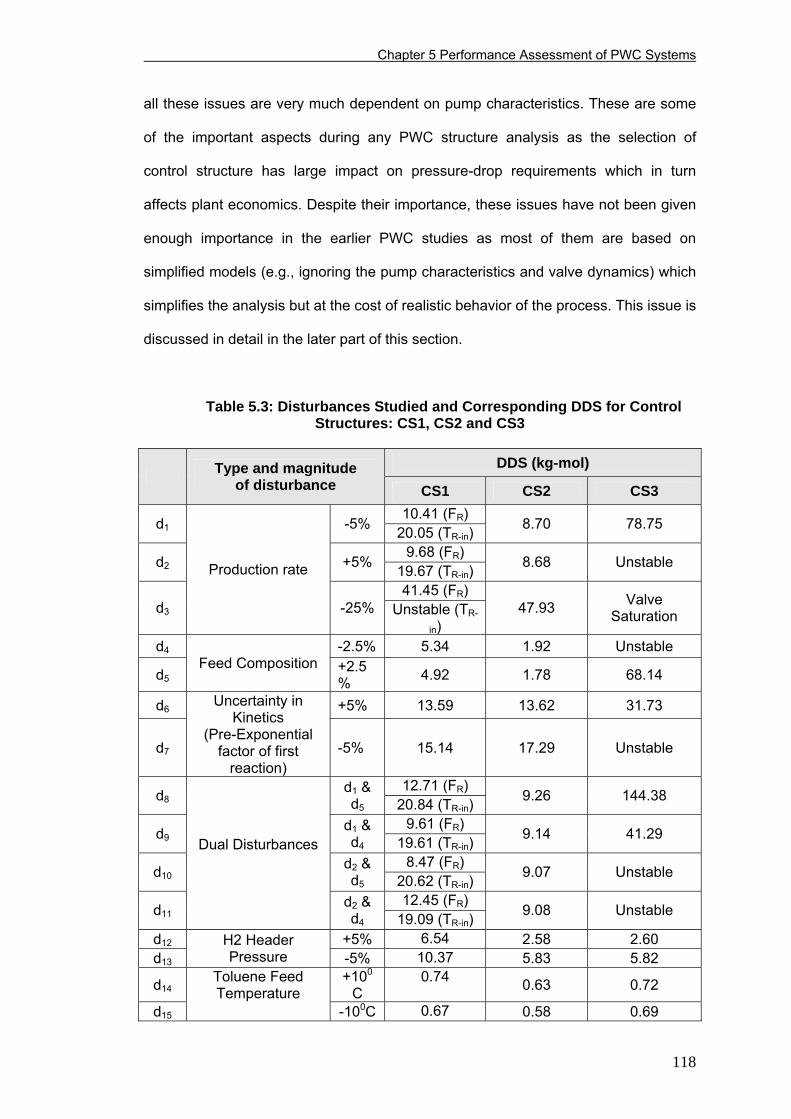
Chapter 5 Performance Assessment of PWC Systems
all these issues are very much dependent on pump characteristics. These are some
of the important aspects during any PWC structure analysis as the selection of
control structure has large impact on pressure-drop requirements which in turn
affects plant economics. Despite their importance, these issues have not been given
enough importance in the earlier PWC studies as most of them are based on
simplified models (e.g., ignoring the pump characteristics and valve dynamics) which
simplifies the analysis but at the cost of realistic behavior of the process. This issue is
discussed in detail in the later part of this section.
Table 5.3: Disturbances Studied and Corresponding DDS for Control Structures: CS1, CS2 and CS3
DDS (kg-mol)
Type and magnitude of disturbance CS1 CS2 CS3
10.41 (FR) d1 -5% 20.05 (TR-in)
8.70 78.75
9.68 (FR) d2 +5% 19.67 (TR-in)
8.68 Unstable
41.45 (FR) d3
Production rate
-25% Unstable (TR-
in) 47.93 Valve
Saturation
d4 -2.5% 5.34 1.92 Unstable
d5Feed Composition +2.5
% 4.92 1.78 68.14
d6 +5% 13.59 13.62 31.73
d7
Uncertainty in Kinetics
(Pre-Exponential factor of first
reaction) -5% 15.14 17.29 Unstable
12.71 (FR) d8
d1 & d5 20.84 (TR-in)
9.26 144.38
9.61 (FR) d9
d1 & d4 19.61 (TR-in)
9.14 41.29
8.47 (FR) d10
d2 & d5 20.62 (TR-in)
9.07 Unstable
12.45 (FR) d11
Dual Disturbances
d2 & d4 19.09 (TR-in)
9.08 Unstable
d12 +5% 6.54 2.58 2.60 d13
H2 Header Pressure -5% 10.37 5.83 5.82
d14+100
C 0.74 0.63 0.72
d15
Toluene Feed Temperature
-100C 0.67 0.58 0.69
118
Chapter 5 Performance Assessment of PWC Systems
5.5.1 Evaluation of CS1 and CS2
CS1 has two potential TPMs: 1) FR, and 2) TR-in. Thus, both the TPMs are
considered in this study, and represented as FR and TR-in in Tables 5.3 to 5.7 based
on what manipulator is used to achieve the throughput changes. It is of interest to
see which one is the better manipulator for CS1. In general, the dynamic behavior of
the process, especially, separation section (i.e., three distillation columns), is very
different for both these TPMs. The changes in vapor flow rate within the three
distillation columns for ±5% change in the throughput (using both the manipulators)
are given in Table 5.4. It can be seen that, with TR-in as the TPM, recycle column is
much more sensitive than the other two columns; change in internal-vapor flow rate
of recycle column is +12.77% compared to -2.85% and +0.58% changes in product
and stabilizer columns respectively. Thus, the robustness of CS1 with TR-in as the
manipulator largely depends on recycle column. On the other hand, with FR as the
TPM, recycle column becomes relatively less sensitive compared to other columns (-
1% change in internal vapor flows of recycle column vs -4.67% and -3.72% changes
in product column and stabilizer respectively for -5% change in the throughput). In
this case, though the impact of the disturbances is transferred to the other columns
(which eventually made product and stabilizer columns relatively more sensitive to
disturbances), none of the columns is as severely affected as the recycle column in
the process with CS1 and TR-in as the TPM. Thus, with FR as the TPM, CS1 is more
robust and handles bigger disturbances.
It can now be concluded that fixing a flow in order to avoid snowball effect,
though a feasible alternative, does not serve the purpose if the TPM is not chosen
appropriately; else, it will only transfer the snowball effect from one part of the
process to another (i.e., from total toluene flow to recycle column in this case).
Similar observation is made by Yu (1999) in case of a simple reactor-separation-
119
Chapter 5 Performance Assessment of PWC Systems
recycle network. On the other hand, with CS2, the effect of disturbances on all three
distillation columns is almost comparable thus making CS2 a balanced control
structure (Table 5.4). The presence of conversion controller is the main reason for
this balanced nature of CS2 (Konda et al., 2005).
With TR-in as the TPM, in the presence of -5% change in the production rate,
as shown in Table 5.4, variation in the vapor loads of the recycle column is much
higher than that of the product and the stabilizer columns (i.e., +12.77% versus -
2.85% and +0.58%). Moreover, the vapor loads in the product column decreased
whereas the vapor loads in the recycle column and the stabilizer increased (Table
5.4). Consequently, there is a significant increase in the steam requirement for the
recycle column’s reboiler (Table 5.5). On the other hand, CS2 and CS1 with FR as
the TPM exhibited relatively more uniform dynamics by almost equally distributing the
impact of the disturbance amongst all the columns (Tables 5.4 and 5.5). Further,
variation in the steam requirement for the recycle column’s reboiler is much less
(Table 5.5). Similarly, changes in the internal liquid flows in the columns are highly
non-uniform if the TR-in is the TPM for CS1; for example, for ±5% changes in the
throughput, the changes in internal liquid flows of different trays of toluene column
are very much different, with a minimum and maximum change of -6% and +12%
respectively. On the other hand, for CS1 with FR as the TPM, the changes are quite
uniform with a minimum and maximum change of 10% and 13% respectively, thereby
exhibiting more linear (internal) column dynamics, and thus a linear controller (such
as a PID type controller) performs better.
120
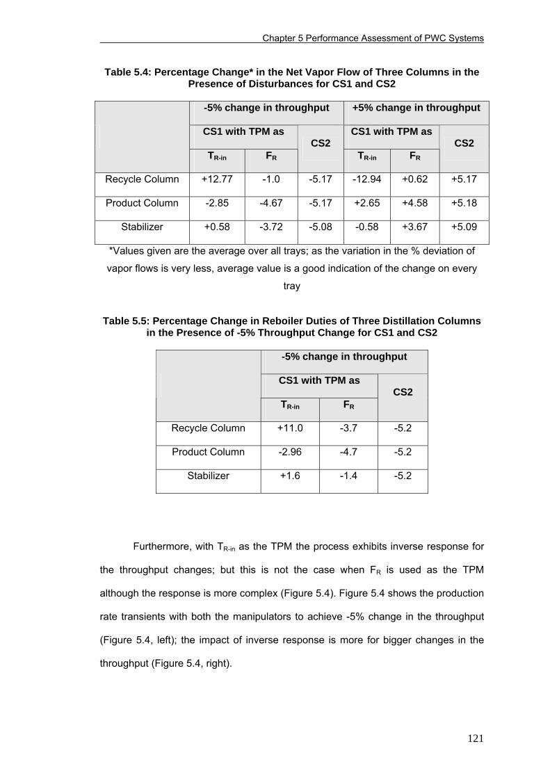
Chapter 5 Performance Assessment of PWC Systems
Table 5.4: Percentage Change* in the Net Vapor Flow of Three Columns in the Presence of Disturbances for CS1 and CS2
-5% change in throughput +5% change in throughput
CS1 with TPM as CS1 with TPM as
TR-in FR
CS2 TR-in FR
CS2
Recycle Column +12.77 -1.0 -5.17 -12.94 +0.62 +5.17
Product Column -2.85 -4.67 -5.17 +2.65 +4.58 +5.18
Stabilizer +0.58 -3.72 -5.08 -0.58 +3.67 +5.09
*Values given are the average over all trays; as the variation in the % deviation of
vapor flows is very less, average value is a good indication of the change on every
tray
Table 5.5: Percentage Change in Reboiler Duties of Three Distillation Columns in the Presence of -5% Throughput Change for CS1 and CS2
-5% change in throughput
CS1 with TPM as
TR-in FR
CS2
Recycle Column +11.0 -3.7 -5.2
Product Column -2.96 -4.7 -5.2
Stabilizer +1.6 -1.4 -5.2
Furthermore, with TR-in as the TPM the process exhibits inverse response for
the throughput changes; but this is not the case when FR is used as the TPM
although the response is more complex (Figure 5.4). Figure 5.4 shows the production
rate transients with both the manipulators to achieve -5% change in the throughput
(Figure 5.4, left); the impact of inverse response is more for bigger changes in the
throughput (Figure 5.4, right).
121
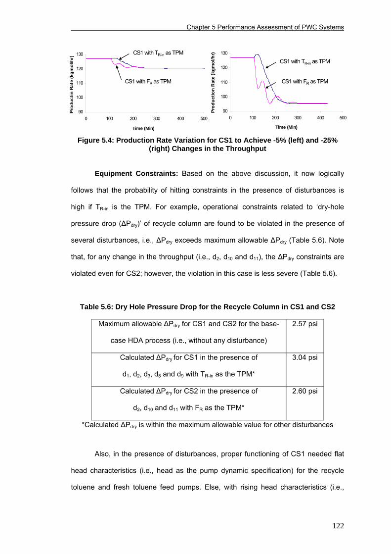
Chapter 5 Performance Assessment of PWC Systems
90
100
110
120
130
0 100 200 300 400 500
Time (Min)
Prod
uctin
Rat
e (k
gmol
/hr)
90
100
110
120
130
0 100 200 300 400 500
Time (Min)
Prod
uctio
n R
ate
(kgm
ol/h
r)CS1 with TR-in as TPMCS1 with TR-in as TPM
CS1 with FR as TPM CS1 with FR as TPM
90
100
110
120
130
0 100 200 300 400 500
Time (Min)
Prod
uctin
Rat
e (k
gmol
/hr)
90
100
110
120
130
0 100 200 300 400 500
Time (Min)
Prod
uctio
n R
ate
(kgm
ol/h
r)CS1 with TR-in as TPMCS1 with TR-in as TPM
CS1 with FR as TPM CS1 with FR as TPM
Figure 5.4: Production Rate Variation for CS1 to Achieve -5% (left) and -25% (right) Changes in the Throughput
Equipment Constraints: Based on the above discussion, it now logically
follows that the probability of hitting constraints in the presence of disturbances is
high if TR-in is the TPM. For example, operational constraints related to ‘dry-hole
pressure drop (ΔPdry)’ of recycle column are found to be violated in the presence of
several disturbances, i.e., ΔPdry exceeds maximum allowable ΔPdry (Table 5.6). Note
that, for any change in the throughput (i.e., d2, d10 and d11), the ΔPdry constraints are
violated even for CS2; however, the violation in this case is less severe (Table 5.6).
Table 5.6: Dry Hole Pressure Drop for the Recycle Column in CS1 and CS2
Maximum allowable ΔPdry for CS1 and CS2 for the base-
case HDA process (i.e., without any disturbance)
2.57 psi
Calculated ΔPdry for CS1 in the presence of
d1, d2, d3, d8 and d9 with TR-in as the TPM*
3.04 psi
Calculated ΔPdry for CS2 in the presence of
d2, d10 and d11 with FR as the TPM*
2.60 psi
*Calculated ΔPdry is within the maximum allowable value for other disturbances
Also, in the presence of disturbances, proper functioning of CS1 needed flat
head characteristics (i.e., head as the pump dynamic specification) for the recycle
toluene and fresh toluene feed pumps. Else, with rising head characteristics (i.e.,
122
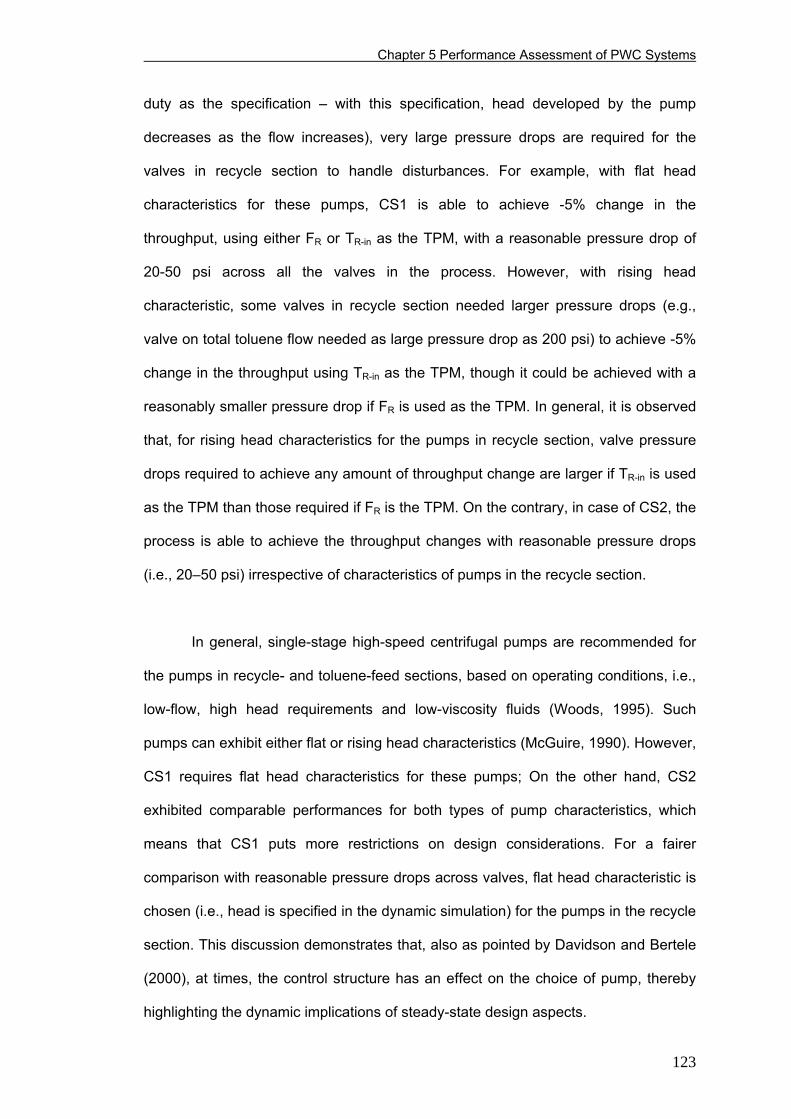
Chapter 5 Performance Assessment of PWC Systems
duty as the specification – with this specification, head developed by the pump
decreases as the flow increases), very large pressure drops are required for the
valves in recycle section to handle disturbances. For example, with flat head
characteristics for these pumps, CS1 is able to achieve -5% change in the
throughput, using either FR or TR-in as the TPM, with a reasonable pressure drop of
20-50 psi across all the valves in the process. However, with rising head
characteristic, some valves in recycle section needed larger pressure drops (e.g.,
valve on total toluene flow needed as large pressure drop as 200 psi) to achieve -5%
change in the throughput using TR-in as the TPM, though it could be achieved with a
reasonably smaller pressure drop if FR is used as the TPM. In general, it is observed
that, for rising head characteristics for the pumps in recycle section, valve pressure
drops required to achieve any amount of throughput change are larger if TR-in is used
as the TPM than those required if FR is the TPM. On the contrary, in case of CS2, the
process is able to achieve the throughput changes with reasonable pressure drops
(i.e., 20–50 psi) irrespective of characteristics of pumps in the recycle section.
In general, single-stage high-speed centrifugal pumps are recommended for
the pumps in recycle- and toluene-feed sections, based on operating conditions, i.e.,
low-flow, high head requirements and low-viscosity fluids (Woods, 1995). Such
pumps can exhibit either flat or rising head characteristics (McGuire, 1990). However,
CS1 requires flat head characteristics for these pumps; On the other hand, CS2
exhibited comparable performances for both types of pump characteristics, which
means that CS1 puts more restrictions on design considerations. For a fairer
comparison with reasonable pressure drops across valves, flat head characteristic is
chosen (i.e., head is specified in the dynamic simulation) for the pumps in the recycle
section. This discussion demonstrates that, also as pointed by Davidson and Bertele
(2000), at times, the control structure has an effect on the choice of pump, thereby
highlighting the dynamic implications of steady-state design aspects.
123
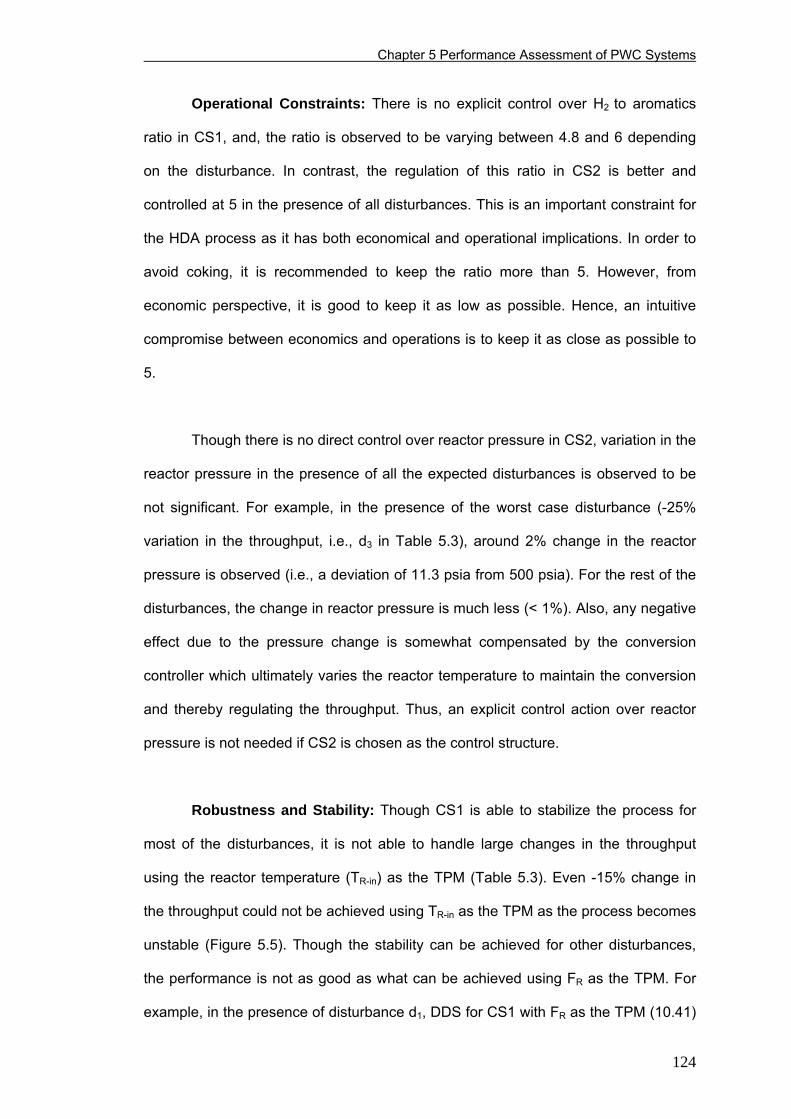
Chapter 5 Performance Assessment of PWC Systems
Operational Constraints: There is no explicit control over H2 to aromatics
ratio in CS1, and, the ratio is observed to be varying between 4.8 and 6 depending
on the disturbance. In contrast, the regulation of this ratio in CS2 is better and
controlled at 5 in the presence of all disturbances. This is an important constraint for
the HDA process as it has both economical and operational implications. In order to
avoid coking, it is recommended to keep the ratio more than 5. However, from
economic perspective, it is good to keep it as low as possible. Hence, an intuitive
compromise between economics and operations is to keep it as close as possible to
5.
Though there is no direct control over reactor pressure in CS2, variation in the
reactor pressure in the presence of all the expected disturbances is observed to be
not significant. For example, in the presence of the worst case disturbance (-25%
variation in the throughput, i.e., d3 in Table 5.3), around 2% change in the reactor
pressure is observed (i.e., a deviation of 11.3 psia from 500 psia). For the rest of the
disturbances, the change in reactor pressure is much less (< 1%). Also, any negative
effect due to the pressure change is somewhat compensated by the conversion
controller which ultimately varies the reactor temperature to maintain the conversion
and thereby regulating the throughput. Thus, an explicit control action over reactor
pressure is not needed if CS2 is chosen as the control structure.
Robustness and Stability: Though CS1 is able to stabilize the process for
most of the disturbances, it is not able to handle large changes in the throughput
using the reactor temperature (TR-in) as the TPM (Table 5.3). Even -15% change in
the throughput could not be achieved using TR-in as the TPM as the process becomes
unstable (Figure 5.5). Though the stability can be achieved for other disturbances,
the performance is not as good as what can be achieved using FR as the TPM. For
example, in the presence of disturbance d1, DDS for CS1 with FR as the TPM (10.41)
124
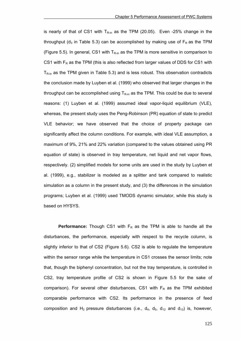
Chapter 5 Performance Assessment of PWC Systems
is nearly of that of CS1 with TR-in as the TPM (20.05). Even -25% change in the
throughput (d3 in Table 5.3) can be accomplished by making use of FR as the TPM
(Figure 5.5). In general, CS1 with TR-in as the TPM is more sensitive in comparison to
CS1 with FR as the TPM (this is also reflected from larger values of DDS for CS1 with
TR-in as the TPM given in Table 5.3) and is less robust. This observation contradicts
the conclusion made by Luyben et al. (1999) who observed that larger changes in the
throughput can be accomplished using TR-in as the TPM. This could be due to several
reasons: (1) Luyben et al. (1999) assumed ideal vapor-liquid equilibrium (VLE),
whereas, the present study uses the Peng-Robinson (PR) equation of state to predict
VLE behavior; we have observed that the choice of property package can
significantly affect the column conditions. For example, with ideal VLE assumption, a
maximum of 9%, 21% and 22% variation (compared to the values obtained using PR
equation of state) is observed in tray temperature, net liquid and net vapor flows,
respectively. (2) simplified models for some units are used in the study by Luyben et
al. (1999), e.g., stabilizer is modeled as a splitter and tank compared to realistic
simulation as a column in the present study, and (3) the differences in the simulation
programs; Luyben et al. (1999) used TMODS dynamic simulator, while this study is
based on HYSYS.
Performance: Though CS1 with FR as the TPM is able to handle all the
disturbances, the performance, especially with respect to the recycle column, is
slightly inferior to that of CS2 (Figure 5.6). CS2 is able to regulate the temperature
within the sensor range while the temperature in CS1 crosses the sensor limits; note
that, though the biphenyl concentration, but not the tray temperature, is controlled in
CS2, tray temperature profile of CS2 is shown in Figure 5.5 for the sake of
comparison). For several other disturbances, CS1 with FR as the TPM exhibited
comparable performance with CS2. Its performance in the presence of feed
composition and H2 pressure disturbances (i.e., d4, d5, d12 and d13) is, however,
125
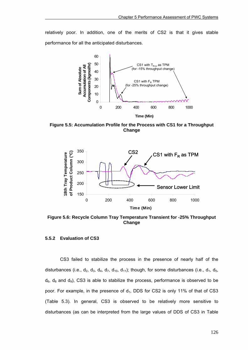
Chapter 5 Performance Assessment of PWC Systems
relatively poor. In addition, one of the merits of CS2 is that it gives stable
performance for all the anticipated disturbances.
0
10
20
30
40
50
60
0 200 400 600 800 1000
Time (Min)
Sum
of A
bsol
ute
Accu
mul
atio
n of
All
Com
pone
nts
(kgm
ol/h
r) CS1 with TR-in as TPM(for -15% throughput change)
CS1 with FR TPM(for -25% throughput change)
0
10
20
30
40
50
60
0 200 400 600 800 1000
Time (Min)
Sum
of A
bsol
ute
Accu
mul
atio
n of
All
Com
pone
nts
(kgm
ol/h
r) CS1 with TR-in as TPM(for -15% throughput change)
CS1 with FR TPM(for -25% throughput change)
Figure 5.5: Accumulation Profile for the Process with CS1 for a Throughput Change
150
200
250
300
350
0 200 400 600 800 1000
Time (Min)
18th
Tra
y Te
mpe
ratu
re
of P
rodu
ct C
olum
n (°
C)
Sensor Lower Limit
CS2 CS1 with FR as TPM
150
200
250
300
350
0 200 400 600 800 1000
Time (Min)
18th
Tra
y Te
mpe
ratu
re
of P
rodu
ct C
olum
n (°
C)
Sensor Lower Limit
CS2 CS1 with FR as TPM
Sensor Lower Limit
CS2 CS1 with FR as TPM
Figure 5.6: Recycle Column Tray Temperature Transient for -25% Throughput Change
5.5.2 Evaluation of CS3
CS3 failed to stabilize the process in the presence of nearly half of the
disturbances (i.e., d2, d3, d4, d7, d10, d11); though, for some disturbances (i.e., d1, d5,
d6, d8 and d9), CS3 is able to stabilize the process, performance is observed to be
poor. For example, in the presence of d1, DDS for CS2 is only 11% of that of CS3
(Table 5.3). In general, CS3 is observed to be relatively more sensitive to
disturbances (as can be interpreted from the large values of DDS of CS3 in Table
126
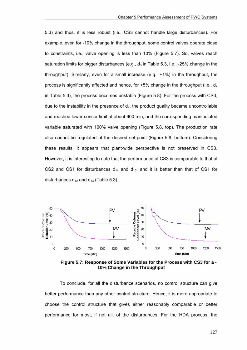
Chapter 5 Performance Assessment of PWC Systems
5.3) and thus, it is less robust (i.e., CS3 cannot handle large disturbances). For
example, even for -10% change in the throughput, some control valves operate close
to constraints, i.e., valve opening is less than 10% (Figure 5.7). So, valves reach
saturation limits for bigger disturbances (e.g., d3 in Table 5.3, i.e., -25% change in the
throughput). Similarly, even for a small increase (e.g., +1%) in the throughput, the
process is significantly affected and hence, for +5% change in the throughput (i.e., d2
in Table 5.3), the process becomes unstable (Figure 5.8). For the process with CS3,
due to the instability in the presence of d2, the product quality became uncontrollable
and reached lower sensor limit at about 900 min; and the corresponding manipulated
variable saturated with 100% valve opening (Figure 5.8, top). The production rate
also cannot be regulated at the desired set-point (Figure 5.8; bottom). Considering
these results, it appears that plant-wide perspective is not preserved in CS3.
However, it is interesting to note that the performance of CS3 is comparable to that of
CS2 and CS1 for disturbances d14 and d15, and it is better than that of CS1 for
disturbances d12 and d13 (Table 5.3).
0
10
20
30
40
50
0 250 500 750 1000 1250 1500
Time (Min)
Prod
uct C
olum
n R
eboi
ler L
evel
(%)
0
10
20
30
40
50
0 250 500 750 1000 1250 1500
Time (Min)
Rec
ycle
Col
umn
Con
dens
er L
evel
(%)PV
MV
PV
MV
0
10
20
30
40
50
0 250 500 750 1000 1250 1500
Time (Min)
Prod
uct C
olum
n R
eboi
ler L
evel
(%)
0
10
20
30
40
50
0 250 500 750 1000 1250 1500
Time (Min)
Rec
ycle
Col
umn
Con
dens
er L
evel
(%)PV
MV
PV
MV
Figure 5.7: Response of Some Variables for the Process with CS3 for a -10% Change in the Throughput
To conclude, for all the disturbance scenarios, no control structure can give
better performance than any other control structure. Hence, it is more appropriate to
choose the control structure that gives either reasonably comparable or better
performance for most, if not all, of the disturbances. For the HDA process, the
127
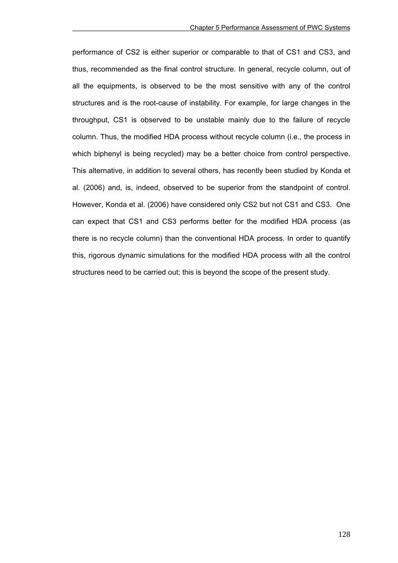
Chapter 5 Performance Assessment of PWC Systems
performance of CS2 is either superior or comparable to that of CS1 and CS3, and
thus, recommended as the final control structure. In general, recycle column, out of
all the equipments, is observed to be the most sensitive with any of the control
structures and is the root-cause of instability. For example, for large changes in the
throughput, CS1 is observed to be unstable mainly due to the failure of recycle
column. Thus, the modified HDA process without recycle column (i.e., the process in
which biphenyl is being recycled) may be a better choice from control perspective.
This alternative, in addition to several others, has recently been studied by Konda et
al. (2006) and, is, indeed, observed to be superior from the standpoint of control.
However, Konda et al. (2006) have considered only CS2 but not CS1 and CS3. One
can expect that CS1 and CS3 performs better for the modified HDA process (as
there is no recycle column) than the conventional HDA process. In order to quantify
this, rigorous dynamic simulations for the modified HDA process with all the control
structures need to be carried out; this is beyond the scope of the present study.
128
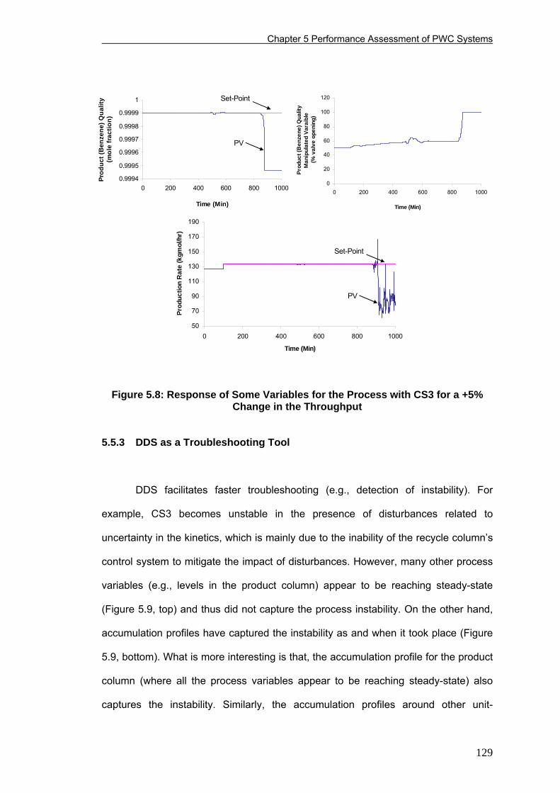
Chapter 5 Performance Assessment of PWC Systems
0.9994
0.9995
0.9996
0.9997
0.9998
0.9999
1
0 200 400 600 800 1000
Time (Min)
Prod
uct (
Ben
zene
) Qua
lity
(mol
e fr
actio
n)
0
20
40
60
80
100
120
0 200 400 600 800 1000
Time (Min)
Prod
uct (
Ben
zene
) Qua
lity
Man
ipul
ated
Var
aibl
e (%
val
ve o
peni
ng)
Set-Point
PV
50
70
90
110
130
150
170
190
0 200 400 600 800 1000
Time (Min)
Prod
uctio
n R
ate
(kgm
ol/h
r)
Set-Point
PV
Figure 5.8: Response of Some Variables for the Process with CS3 for a +5% Change in the Throughput
5.5.3 DDS as a Troubleshooting Tool
DDS facilitates faster troubleshooting (e.g., detection of instability). For
example, CS3 becomes unstable in the presence of disturbances related to
uncertainty in the kinetics, which is mainly due to the inability of the recycle column’s
control system to mitigate the impact of disturbances. However, many other process
variables (e.g., levels in the product column) appear to be reaching steady-state
(Figure 5.9, top) and thus did not capture the process instability. On the other hand,
accumulation profiles have captured the instability as and when it took place (Figure
5.9, bottom). What is more interesting is that, the accumulation profile for the product
column (where all the process variables appear to be reaching steady-state) also
captures the instability. Similarly, the accumulation profiles around other unit-
129
Chapter 5 Performance Assessment of PWC Systems
operations (e.g., reactor, stabilizer and benzene column) also capture instability even
though the associated process variables appear to be reaching steady-state (Figure
5.10). This emphasizes the fact that accumulation profile preserves the plant-wide
perspective and thus it can be a better measure for plant-wide performance
assessment. At times, depending on the severity of the accumulation and process
complexity, it might take hours or even days to recognize any instability through the
process variables. On the other hand, accumulation profiles (either local or plant-
wide) signal instability quickly if there is instability anywhere in the plant. For
example, from Figure 5.8, the process instability can be identified only after 900 min
of operation. On the other hand, as shown in Figure 5.11, instability can be identified
soon after 400 min of operation from accumulation profiles of the entire plant.
0
1
2
3
4
5
0 250 500 750 1000 1250 1500
Time (Min)
Sum
of A
bsol
ute
Acc
umul
atio
n of
All
Com
pone
nts
(kgm
ol/h
r)
45
50
55
60
65
70
75
0 250 500 750 1000 1250 1500
Time (Min)
Reb
oile
r Lev
el (%
)
40
45
50
55
60
0 250 500 750 1000 1250 1500
Time (Min)
Con
dens
er L
evel
(%)
MVMV
PV PV
for the entire process
for the product column only
for the entire process
for the product column only
Figure 5.9: Product Column Level (above) and Accumulation (below) Profiles
for the Process with CS3 in the presence of Uncertainty in the Reaction Kinetics (i.e., d7)
130
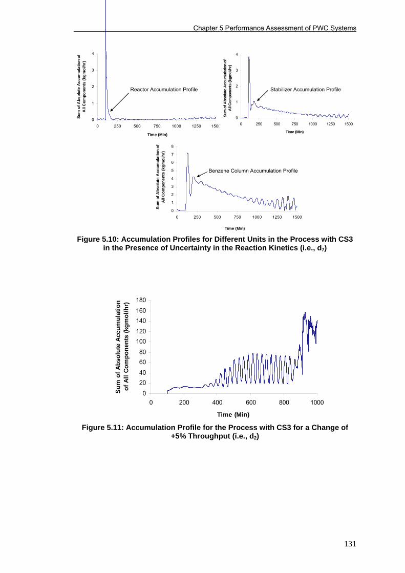
Chapter 5 Performance Assessment of PWC Systems
0
1
2
3
4
5
6
7
8
0 250 500 750 1000 1250 1500
Time (Min)
Sum
of A
bsol
ute
Acc
umul
atio
n of
All
Com
pone
nts
(kgm
ol/h
r)
0
1
2
3
4
0 250 500 750 1000 1250 1500
Time (Min)
Sum
of A
bsol
ute
Acc
umul
atio
n of
All
Com
pone
nts
(kgm
ol/h
r)
0
1
2
3
4
0 250 500 750 1000 1250 1500
Time (Min)
Sum
of A
bsol
ute
Acc
umul
atio
n of
A
ll C
ompo
nent
s (k
gmol
/hr)
Reactor Accumulation Profile
Benzene Column Accumulation Profile
Stabilizer Accumulation Profile
0
1
2
3
4
5
6
7
8
0 250 500 750 1000 1250 1500
Time (Min)
Sum
of A
bsol
ute
Acc
umul
atio
n of
All
Com
pone
nts
(kgm
ol/h
r)
0
1
2
3
4
0 250 500 750 1000 1250 1500
Time (Min)
Sum
of A
bsol
ute
Acc
umul
atio
n of
All
Com
pone
nts
(kgm
ol/h
r)
0
1
2
3
4
0 250 500 750 1000 1250 1500
Time (Min)
Sum
of A
bsol
ute
Acc
umul
atio
n of
A
ll C
ompo
nent
s (k
gmol
/hr)
Reactor Accumulation Profile
Benzene Column Accumulation Profile
Stabilizer Accumulation Profile
Figure 5.10: Accumulation Profiles for Different Units in the Process with CS3 in the Presence of Uncertainty in the Reaction Kinetics (i.e., d7)
0
2040
6080
100120
140160
180
0 200 400 600 800 1000
Time (Min)
Sum
of A
bsol
ute
Acc
umul
atio
n of
All
Com
pone
nts
(kgm
ol/h
r)
Figure 5.11: Accumulation Profile for the Process with CS3 for a Change of +5% Throughput (i.e., d2)
131
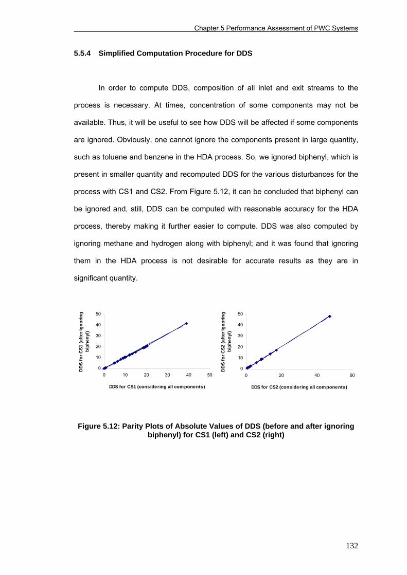
Chapter 5 Performance Assessment of PWC Systems
5.5.4 Simplified Computation Procedure for DDS
In order to compute DDS, composition of all inlet and exit streams to the
process is necessary. At times, concentration of some components may not be
available. Thus, it will be useful to see how DDS will be affected if some components
are ignored. Obviously, one cannot ignore the components present in large quantity,
such as toluene and benzene in the HDA process. So, we ignored biphenyl, which is
present in smaller quantity and recomputed DDS for the various disturbances for the
process with CS1 and CS2. From Figure 5.12, it can be concluded that biphenyl can
be ignored and, still, DDS can be computed with reasonable accuracy for the HDA
process, thereby making it further easier to compute. DDS was also computed by
ignoring methane and hydrogen along with biphenyl; and it was found that ignoring
them in the HDA process is not desirable for accurate results as they are in
significant quantity.
0
10
20
30
40
50
0 10 20 30 40 50
DDS for CS1 (considering all components)
DD
S fo
r CS1
(aft
er ig
norin
g bi
phen
yl)
0
10
20
30
40
50
0 20 40
DDS for CS2 (considering all components)
DD
S fo
r CS2
(aft
er ig
norin
g bi
phen
yl)
60
Figure 5.12: Parity Plots of Absolute Values of DDS (before and after ignoring biphenyl) for CS1 (left) and CS2 (right)
132
Chapter 5 Performance Assessment of PWC Systems
5.6 Summary
A performance metric, DDS, is proposed based on component accumulation
profiles which is then successfully used to assess the performance of three PWC
systems for the HDA process using rigorous nonlinear dynamic simulation. As
discussed in Section 5.2, DDS has several advantages; some of them are: DDS is
equally applicable to linear and nonlinear processes, computation procedure of DDS
remains the same irrespective of the control structure, DDS can be computed easily
using rigorous process simulators, and it facilitates early detection of instability.
From the preliminary studies, it is noted that the DDS is proportionately
related to control effort (i.e., control valve movement) but further study needs to be
carried out to quantify this observation. In addition, it should be noted that DDS used
in this study gives equal priority to all the components and also to the positive and
negative deviations. Hence, if these assumptions are not true for any process (e.g., if
some components are measured at ppm level while others are not), DDS should be
appropriately modified, perhaps by considering functions of accumulation of
components while computing DDS. However, such a procedure can be process-
specific (e.g., what should be the function?) and further investigation needs to be
carried out before coming to a conclusion. Since DDS is more fundamentally defined
based on the accumulation in the component material balances, it is more useful for
plant-wide performance analysis. For example, the DDS values over the subsections
of the plant, after normalization, are additive (in order to compute DDS over the entire
process). On the other hand, IAE values are not additive as they can be defined for
any process variable (e.g., temperature, pressure, composition or levels). Though,
DDS do not directly capture the variation in all these process variables, it indirectly
captures the impact through accumulation profiles as any change in these process
133
Chapter 5 Performance Assessment of PWC Systems
variables always effects component material balances. But the normalization of DDS
values over different sections of the plant, on the basis of either section inventory or
flows, needs further investigation so that it can be generalized.
Dynamic performance of three PWC systems (CS1, CS2 and CS3) for the
HDA process in the presence of several anticipated disturbances shows that they
exhibit entirely different behavior. In general, CS2 (the balanced control structure with
the fixed-feed TPM), is observed to be offering superior or comparable performance
over CS1 (control structure with the internal TPM) and CS3 (on-demand control
structure). In addition, satisfaction of operating constraints (such as H2 to aromatics
ratio and dry-hole pressure drops in distillation columns) in CS2 is better, and CS2 is
more flexible from steady-state design standpoint (e.g., choice of pump
characteristics). The performance of CS1 is found to be largely dependent on the
choice of TPM. With FR as the TPM, the performance of CS1 is comparable to that of
CS2 for many disturbances; with TR-in as the TPM, however, the process is more
sensitive to disturbances and thus less robust. CS3 exhibited very slow dynamics
and is more sensitive to the disturbances; thus, it is not able to stabilize the process
for most of the anticipated disturbances. Despite these advantages, the use of CS2
may be hindered as it requires more composition measurements. However,
considering the advances in composition analyzer technology and its increasing
industrial applications, one can foresee that it will be less of a concern
134
Chapter 6 Plant-Wide Interaction of Design and Control
CHAPTER 6
PLANT-WIDE INTERACTION OF DESIGN AND CONTROL*
Integration of process design and control has been receiving growing interest
in recent years to reap both economic and operational benefits. Thus, in this chapter,
a modified sequential approach consisting of two stages and combining rigorous
nonlinear simulation with heuristics is proposed for integrated design and control of
industrial processes. In the first (i.e., design) stage, several alternatives are
systematically generated and ranked based on economics. A few top-ranked
alternatives from the design stage are then forwarded to the second (i.e., control)
stage for further analysis on their dynamics to arrive at the best process that is
economical as well as easy to operate. Nonlinear simulation is combined with
heuristics for realistic analysis in each stage. The control system performance
measure, namely, dynamic disturbance sensitivity (DDS), which was proposed in
Chapter 5, is used to assess the dynamic performance of process designs and
control structures. Application of the proposed approach to the HDA process is
described in detail. The dynamics of the most economical process alternative are
found to be inferior to those of slightly less economical alternatives, which highlight
the need for plant-wide studies on the interaction of design and control.
6.1 Introduction
Design engineers try to design the most economical processes while control
engineers need processes that are the best operable. However, many a times, the
objectives of these two groups, design and control, may contradict. For example,
* This chapter is based on the paper - Konda, N.V.S.N.M., Rangaiah, G.P. and Lim, D.K.H. Optimal Process Design and Effective Plant-Wide Control of Industrial Processes by Simulation-based Heuristic Approach, Ind. Eng. Chem. Res., 45, pp. 5955-5970. 2006.
135
Chapter 6 Plant-Wide Interaction of Design and Control
economically optimal processes may be difficult to control and vice versa, in which
case, a compromised solution has to be developed. Hence, it is important to
understand the interaction effects between design and control in order to be able to
strike the right balance for overall good results (Seferlis and Georgiadis, 2004; Seider
et al., 2004). Interaction between design and control in the context of single units has
been studied by researchers over the last couple of decades. However, relatively
fewer attempts have been made on the interaction effects between process design
and PWC system design. One obvious reason for this is the inherent complexity of
large-scale industrial processes. In particular, processes with recycles introduce
difficulties during process design as well as control system design (Kumar and
Daoutidis, 2002). Analysis would be more complicated and rigorous treatment is
needed before finalizing the design. Thus, integrated design and control from the
plant-wide perspective is needed, which is precisely the subject of this chapter.
Although, there have been several attempts on design and control in the
recent past (Luyben, 2000b; Reyes and Luyben, 2000 & 2001; Chen and Yu, 2003;
Chien et al., 2004), most of them presume that the design and/or control alternatives
are somehow available. In contrast, the present work systematically generates
several design alternatives and then designs effective control systems for the
attractive alternatives. Several researchers studied the interaction of design and
control for hypothetical processes with a given process design and control structure
(Grassi, 1993; Lyman and Luyben, 1996; Wu and Yu, 1997; Luyben, 2000c & 2001;
Cheng and Yu, 2003); however, their primary importance is on the effect of
parametric decisions on control. Present work aims at generating several process
alternatives and studying the impact of both structural and parametric decisions on
control from the plant-wide perspective, using rigorous nonlinear models.
136
Chapter 6 Plant-Wide Interaction of Design and Control
Integrated design and control approaches can be broadly classified into two
categories: (1) simultaneous design and control, and (2) sequential design and
control (Meeuse and Grievink, 2004). In the former approach, control aspects are
considered during each stage of design. The simultaneous approaches can further
be classified based on (i) controllability measures and (ii) optimization. In the former,
controllability metrics are used to gauge the ease of control of a particular process
design. However, most often, this analysis is performed using either steady-state or
linear dynamic models, which usually introduces significant approximations and,
hence might not be able to characterize dynamic behavior of plants with sufficient
accuracy (Sakizlis et al., 2004). The optimization-based methods have been
successfully applied to simple problems involving a small number of units (Luyben
and Floudas, 1994; Perkins and Walsh, 1996; Kookos and Perkins, 2001b).
However, their application to large-scale plants becomes cumbersome, because of
the large combinatorial explosion of alternatives. Moreover, using simultaneous
methods, it is not always possible to take the best possible control decision during
the initial stages of design, because of the lack of sufficient information. Hence, these
decisions, which were taken in the early stages, may have to be revised in the later
stages. In addition, as the best alternative would not surface until the designer
explores the entire search space, typically, every process alternative would have to
be considered in both the design and control stages. This can be extremely time-
consuming, especially in the context of PWC, because economically unattractive
alternatives would also be studied from control viewpoint.
In the sequential approach, design and control are performed sequentially
(e.g., Alhammadi and Romagnoli, 2004). This approach is relatively simple and
equally applicable, even to complex processes; its primary limitation is that process
design is finalized before the controllability analysis is carried out. So, there is a
possibility that one might miss out the process design alternative that is better
137
Chapter 6 Plant-Wide Interaction of Design and Control
controllable with little additional economic penalty. In addition, the process design,
which is finalized based only on steady-state economic considerations, may have
severe operational problems. Hence, in the proposed approach, we select a few
potential design alternatives (instead of only one) that are worthy of consideration for
further controllability analysis. By doing so, the primary limitation of the traditional
sequential approach could be avoided. A similar approach has been used by
Narraway et al. (1991) to understand the interaction between design and control of a
simple process employing mathematical tools on linearized models. However,
nonlinear dynamic models are not considered in their study.
The proposed approach is based on heuristics and simulation to achieve
synergistic benefits. As heuristics cannot always be relied upon, powerful process
simulators are employed as an integral part of this approach, to ensure reliability.
Process simulators for dynamic studies were not used extensively in the past.
However, recent advancements in the computing technology boosted their
capabilities, which, in turn furthered studies on plant-wide analysis (Luyben, 2002).
Process simulators offer a good platform to study complex processes more
effectively. Hence, the present study is based on a process simulator, namely,
HYSYS, which has both the design and control capabilities. The designer can
seamlessly move to dynamic mode from steady state, and make use of essentially
the same model in both the modes. Such a feature can greatly facilitate studies on
integrated design and control especially in the plant-wide context, and, hence,
HYSYS is chosen for the present study. However, the analysis is generic and
applicable to any other commercial process simulator that has got similar capabilities
of design and control. The proposed sequential approach has two stages: (i) process
design and (ii) control system design, which are discussed below.
138
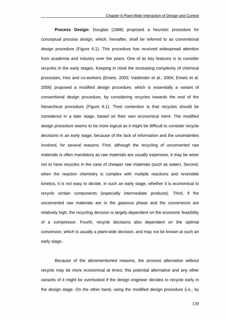
Chapter 6 Plant-Wide Interaction of Design and Control
Process Design: Douglas (1988) proposed a heuristic procedure for
conceptual process design, which, hereafter, shall be referred to as conventional
design procedure (Figure 6.1). This procedure has received widespread attention
from academia and industry over the years. One of its key features is to consider
recycles in the early stages. Keeping in mind the increasing complexity of chemical
processes, Hoo and co-workers (Emets, 2003; Vasbinder et al., 2004; Emets et al.
2006) proposed a modified design procedure, which is essentially a variant of
conventional design procedure, by considering recycles towards the end of the
hierarchical procedure (Figure 6.1). Their contention is that recycles should be
considered in a later stage, based on their own economical merit. The modified
design procedure seems to be more logical as it might be difficult to consider recycle
decisions in an early stage, because of the lack of information and the uncertainties
involved, for several reasons. First, although the recycling of unconverted raw
materials is often mandatory as raw materials are usually expensive, it may be wiser
not to have recycles in the case of cheaper raw materials (such as water). Second,
when the reaction chemistry is complex with multiple reactions and reversible
kinetics, it is not easy to decide, in such an early stage, whether it is economical to
recycle certain components (especially intermediate products). Third, if the
unconverted raw materials are in the gaseous phase and the conversions are
relatively high, the recycling decision is largely dependent on the economic feasibility
of a compressor. Fourth, recycle decisions also dependent on the optimal
conversion, which is usually a plant-wide decision, and may not be known at such an
early stage.
Because of the aforementioned reasons, the process alternative without
recycle may be more economical at times; this potential alternative and any other
variants of it might be overlooked if the design engineer decides to recycle early in
the design stage. On the other hand, using the modified design procedure (i.e., by
139
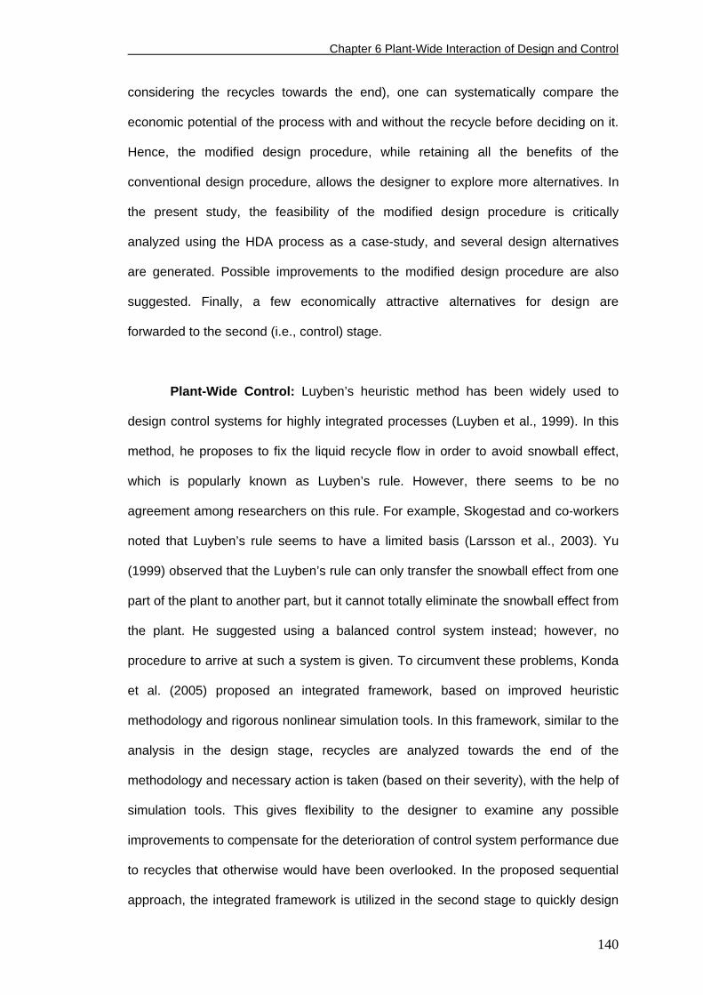
Chapter 6 Plant-Wide Interaction of Design and Control
considering the recycles towards the end), one can systematically compare the
economic potential of the process with and without the recycle before deciding on it.
Hence, the modified design procedure, while retaining all the benefits of the
conventional design procedure, allows the designer to explore more alternatives. In
the present study, the feasibility of the modified design procedure is critically
analyzed using the HDA process as a case-study, and several design alternatives
are generated. Possible improvements to the modified design procedure are also
suggested. Finally, a few economically attractive alternatives for design are
forwarded to the second (i.e., control) stage.
Plant-Wide Control: Luyben’s heuristic method has been widely used to
design control systems for highly integrated processes (Luyben et al., 1999). In this
method, he proposes to fix the liquid recycle flow in order to avoid snowball effect,
which is popularly known as Luyben’s rule. However, there seems to be no
agreement among researchers on this rule. For example, Skogestad and co-workers
noted that Luyben’s rule seems to have a limited basis (Larsson et al., 2003). Yu
(1999) observed that the Luyben’s rule can only transfer the snowball effect from one
part of the plant to another part, but it cannot totally eliminate the snowball effect from
the plant. He suggested using a balanced control system instead; however, no
procedure to arrive at such a system is given. To circumvent these problems, Konda
et al. (2005) proposed an integrated framework, based on improved heuristic
methodology and rigorous nonlinear simulation tools. In this framework, similar to the
analysis in the design stage, recycles are analyzed towards the end of the
methodology and necessary action is taken (based on their severity), with the help of
simulation tools. This gives flexibility to the designer to examine any possible
improvements to compensate for the deterioration of control system performance due
to recycles that otherwise would have been overlooked. In the proposed sequential
approach, the integrated framework is utilized in the second stage to quickly design
140
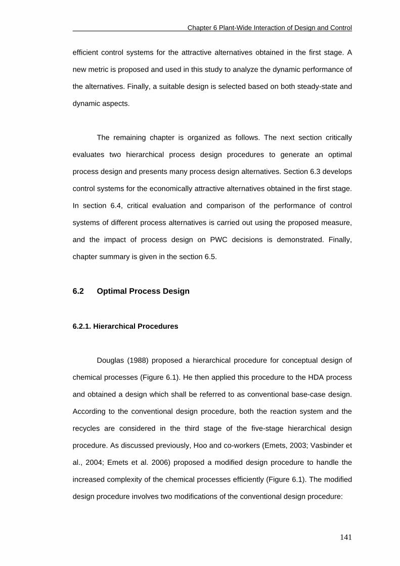
Chapter 6 Plant-Wide Interaction of Design and Control
efficient control systems for the attractive alternatives obtained in the first stage. A
new metric is proposed and used in this study to analyze the dynamic performance of
the alternatives. Finally, a suitable design is selected based on both steady-state and
dynamic aspects.
The remaining chapter is organized as follows. The next section critically
evaluates two hierarchical process design procedures to generate an optimal
process design and presents many process design alternatives. Section 6.3 develops
control systems for the economically attractive alternatives obtained in the first stage.
In section 6.4, critical evaluation and comparison of the performance of control
systems of different process alternatives is carried out using the proposed measure,
and the impact of process design on PWC decisions is demonstrated. Finally,
chapter summary is given in the section 6.5.
6.2 Optimal Process Design
6.2.1. Hierarchical Procedures
Douglas (1988) proposed a hierarchical procedure for conceptual design of
chemical processes (Figure 6.1). He then applied this procedure to the HDA process
and obtained a design which shall be referred to as conventional base-case design.
According to the conventional design procedure, both the reaction system and the
recycles are considered in the third stage of the five-stage hierarchical design
procedure. As discussed previously, Hoo and co-workers (Emets, 2003; Vasbinder et
al., 2004; Emets et al. 2006) proposed a modified design procedure to handle the
increased complexity of the chemical processes efficiently (Figure 6.1). The modified
design procedure involves two modifications of the conventional design procedure:
141
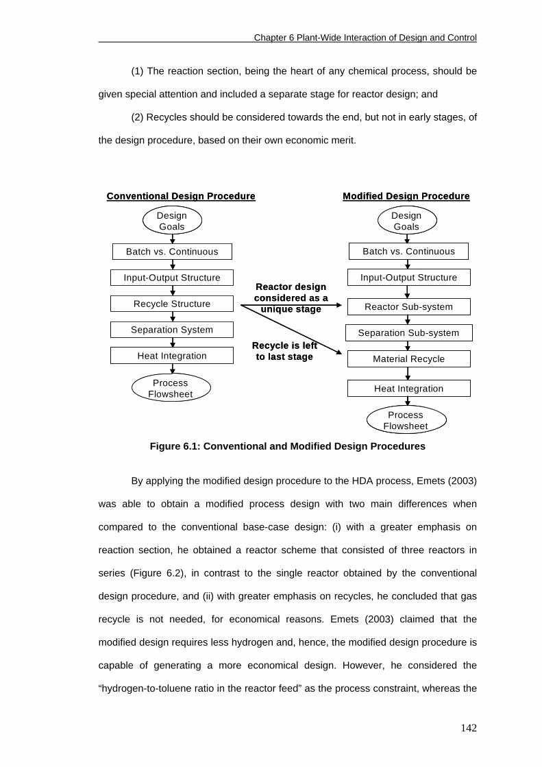
Chapter 6 Plant-Wide Interaction of Design and Control
(1) The reaction section, being the heart of any chemical process, should be
given special attention and included a separate stage for reactor design; and
(2) Recycles should be considered towards the end, but not in early stages, of
the design procedure, based on their own economic merit.
Batch vs. Continuous
Input-Output Structure
Recycle Structure
Separation System
Heat Integration
Batch vs. Continuous
Input-Output Structure
Reactor Sub-system
Separation Sub-system
Material Recycle
Heat Integration
Conventional Design Procedure Modified Design Procedure
Recycle is left to last stage
Reactor design considered as a
unique stage
Design Goals
Design Goals
Process Flowsheet
Process Flowsheet
Batch vs. Continuous
Input-Output Structure
Recycle Structure
Separation System
Heat Integration
Batch vs. Continuous
Input-Output Structure
Reactor Sub-system
Separation Sub-system
Material Recycle
Heat Integration
Conventional Design Procedure Modified Design Procedure
Recycle is left to last stage
Reactor design considered as a
unique stage
Design GoalsDesign Goals
Design GoalsDesign Goals
Process Flowsheet
Process FlowsheetProcess
Flowsheet
Figure 6.1: Conventional and Modified Design Procedures
By applying the modified design procedure to the HDA process, Emets (2003)
was able to obtain a modified process design with two main differences when
compared to the conventional base-case design: (i) with a greater emphasis on
reaction section, he obtained a reactor scheme that consisted of three reactors in
series (Figure 6.2), in contrast to the single reactor obtained by the conventional
design procedure, and (ii) with greater emphasis on recycles, he concluded that gas
recycle is not needed, for economical reasons. Emets (2003) claimed that the
modified design requires less hydrogen and, hence, the modified design procedure is
capable of generating a more economical design. However, he considered the
“hydrogen-to-toluene ratio in the reactor feed” as the process constraint, whereas the
142
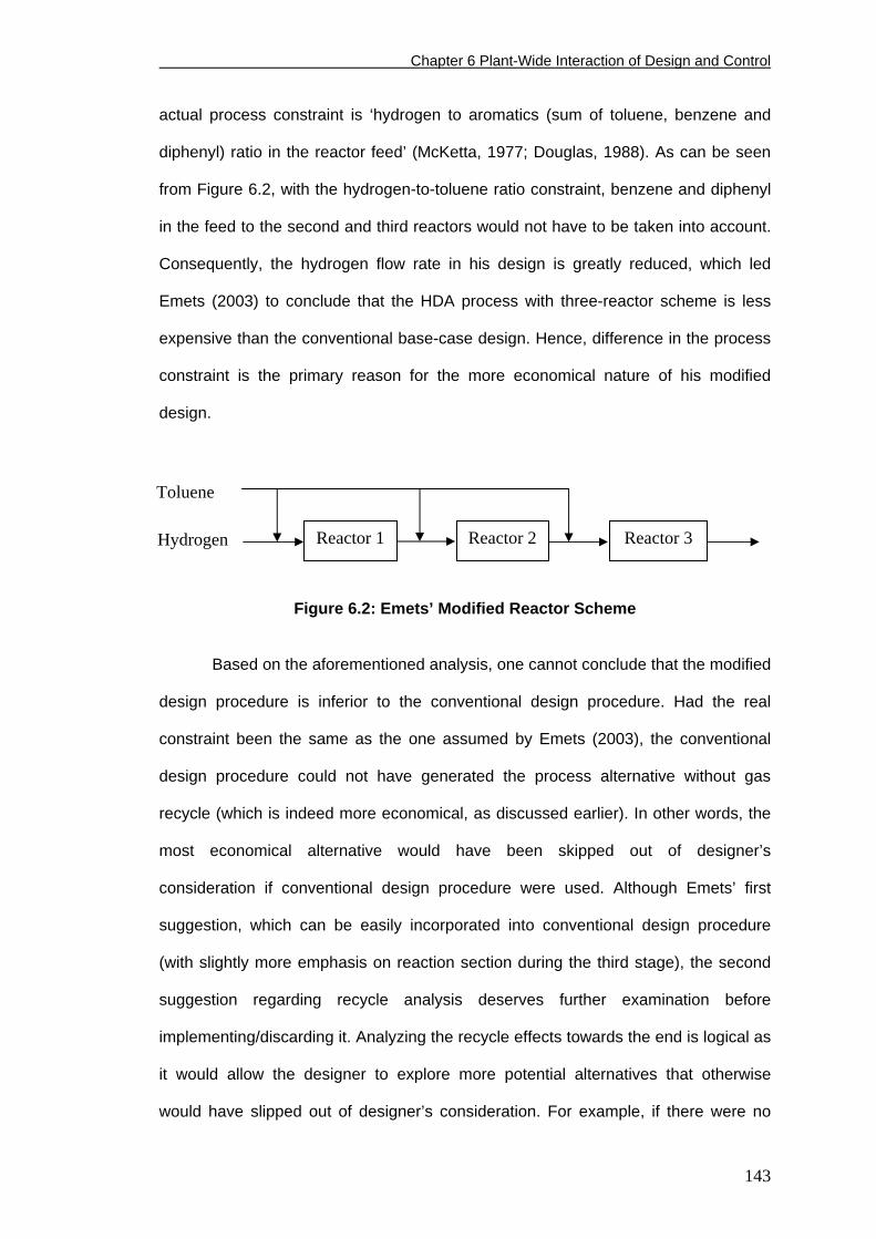
Chapter 6 Plant-Wide Interaction of Design and Control
actual process constraint is ‘hydrogen to aromatics (sum of toluene, benzene and
diphenyl) ratio in the reactor feed’ (McKetta, 1977; Douglas, 1988). As can be seen
from Figure 6.2, with the hydrogen-to-toluene ratio constraint, benzene and diphenyl
in the feed to the second and third reactors would not have to be taken into account.
Consequently, the hydrogen flow rate in his design is greatly reduced, which led
Emets (2003) to conclude that the HDA process with three-reactor scheme is less
expensive than the conventional base-case design. Hence, difference in the process
constraint is the primary reason for the more economical nature of his modified
design.
Toluene
Reactor 1 Reactor 2 Reactor 3 Hydrogen
Figure 6.2: Emets’ Modified Reactor Scheme
Based on the aforementioned analysis, one cannot conclude that the modified
design procedure is inferior to the conventional design procedure. Had the real
constraint been the same as the one assumed by Emets (2003), the conventional
design procedure could not have generated the process alternative without gas
recycle (which is indeed more economical, as discussed earlier). In other words, the
most economical alternative would have been skipped out of designer’s
consideration if conventional design procedure were used. Although Emets’ first
suggestion, which can be easily incorporated into conventional design procedure
(with slightly more emphasis on reaction section during the third stage), the second
suggestion regarding recycle analysis deserves further examination before
implementing/discarding it. Analyzing the recycle effects towards the end is logical as
it would allow the designer to explore more potential alternatives that otherwise
would have slipped out of designer’s consideration. For example, if there were no
143
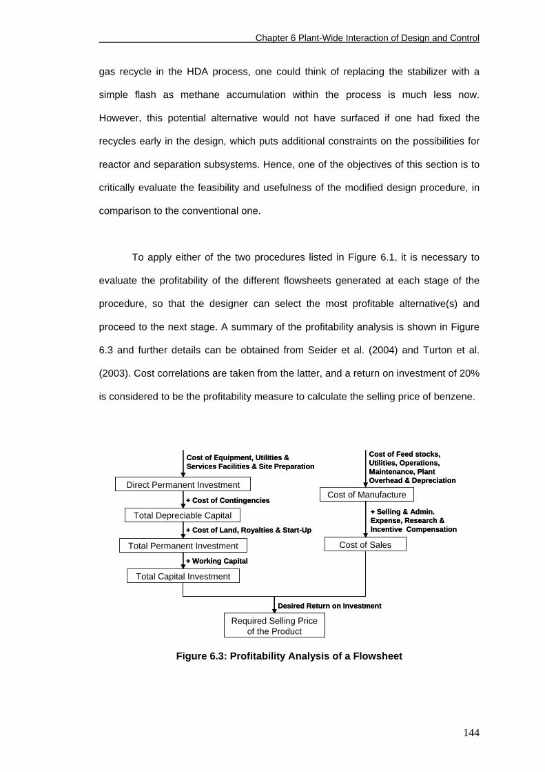
Chapter 6 Plant-Wide Interaction of Design and Control
gas recycle in the HDA process, one could think of replacing the stabilizer with a
simple flash as methane accumulation within the process is much less now.
However, this potential alternative would not have surfaced if one had fixed the
recycles early in the design, which puts additional constraints on the possibilities for
reactor and separation subsystems. Hence, one of the objectives of this section is to
critically evaluate the feasibility and usefulness of the modified design procedure, in
comparison to the conventional one.
To apply either of the two procedures listed in Figure 6.1, it is necessary to
evaluate the profitability of the different flowsheets generated at each stage of the
procedure, so that the designer can select the most profitable alternative(s) and
proceed to the next stage. A summary of the profitability analysis is shown in Figure
6.3 and further details can be obtained from Seider et al. (2004) and Turton et al.
(2003). Cost correlations are taken from the latter, and a return on investment of 20%
is considered to be the profitability measure to calculate the selling price of benzene.
Direct Permanent Investment
Total Depreciable Capital
Total Permanent Investment
Total Capital Investment
+ Cost of Contingencies
Cost of Equipment, Utilities & Services Facilities & Site Preparation
+ Cost of Land, Royalties & Start-Up
+ Working Capital
Cost of Manufacture
Cost of Sales
+ Selling & Admin. Expense, Research & Incentive Compensation
Cost of Feed stocks, Utilities, Operations, Maintenance, Plant Overhead & Depreciation
Required Selling Price of the Product
Desired Return on Investment
Figure 6.3: Profitability Analysis of a Flowsheet
144
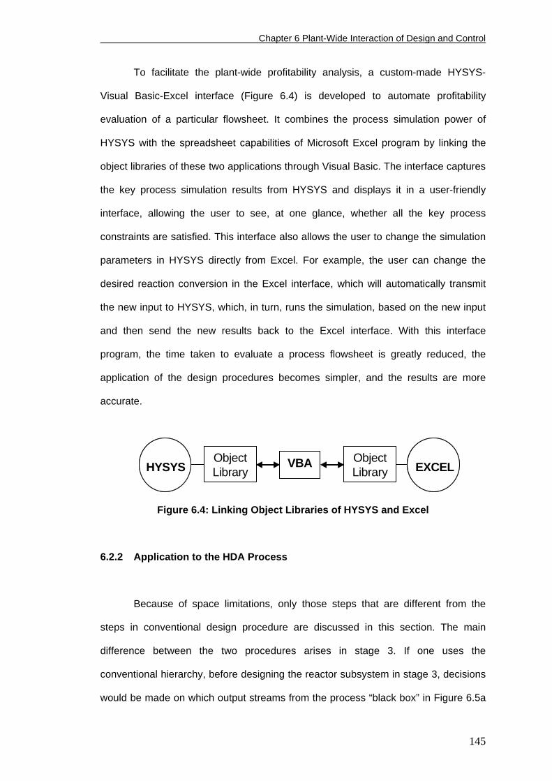
Chapter 6 Plant-Wide Interaction of Design and Control
To facilitate the plant-wide profitability analysis, a custom-made HYSYS-
Visual Basic-Excel interface (Figure 6.4) is developed to automate profitability
evaluation of a particular flowsheet. It combines the process simulation power of
HYSYS with the spreadsheet capabilities of Microsoft Excel program by linking the
object libraries of these two applications through Visual Basic. The interface captures
the key process simulation results from HYSYS and displays it in a user-friendly
interface, allowing the user to see, at one glance, whether all the key process
constraints are satisfied. This interface also allows the user to change the simulation
parameters in HYSYS directly from Excel. For example, the user can change the
desired reaction conversion in the Excel interface, which will automatically transmit
the new input to HYSYS, which, in turn, runs the simulation, based on the new input
and then send the new results back to the Excel interface. With this interface
program, the time taken to evaluate a process flowsheet is greatly reduced, the
application of the design procedures becomes simpler, and the results are more
accurate.
HYSYSObjectLibrary EXCEL
ObjectLibrary
VBAHYSYSObjectLibrary EXCEL
ObjectLibrary
VBA
Figure 6.4: Linking Object Libraries of HYSYS and Excel
6.2.2 Application to the HDA Process
Because of space limitations, only those steps that are different from the
steps in conventional design procedure are discussed in this section. The main
difference between the two procedures arises in stage 3. If one uses the
conventional hierarchy, before designing the reactor subsystem in stage 3, decisions
would be made on which output streams from the process “black box” in Figure 6.5a
145
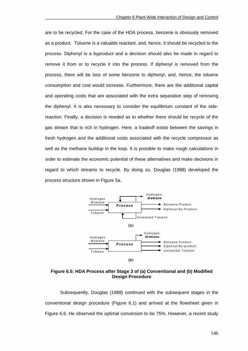
Chapter 6 Plant-Wide Interaction of Design and Control
are to be recycled. For the case of the HDA process, benzene is obviously removed
as a product. Toluene is a valuable reactant, and, hence, it should be recycled to the
process. Diphenyl is a byproduct and a decision should also be made in regard to
remove it from or to recycle it into the process. If diphenyl is removed from the
process, there will be loss of some benzene to diphenyl, and, hence, the toluene
consumption and cost would increase. Furthermore, there are the additional capital
and operating costs that are associated with the extra separation step of removing
the diphenyl. It is also necessary to consider the equilibrium constant of the side-
reaction. Finally, a decision is needed as to whether there should be recycle of the
gas stream that is rich in hydrogen. Here, a tradeoff exists between the savings in
fresh hydrogen and the additional costs associated with the recycle compressor as
well as the methane buildup in the loop. It is possible to make rough calculations in
order to estimate the economic potential of these alternatives and make decisions in
regard to which streams to recycle. By doing so, Douglas (1988) developed the
process structure shown in Figure 5a.
D iphenyl B y-productU nreac ted T o lueneT o luene
H ydrogen M ethane
P rocess
H ydrogen, M ethane
B enzene P roduct
U nreac ted T o lueneT o luene
H ydrogen M ethane
P rocess
H ydrogen, M ethane
B enzene P roductD iphenyl B y-P roduct
(a )
(b )
D iphenyl B y-productU nreac ted T o lueneT o luene
H ydrogen M ethane
P rocess
H ydrogen, M ethane
B enzene P roductD iphenyl B y-productU nreac ted T o lueneT o luene
H ydrogen M ethane
P rocess
H ydrogen, M ethane
B enzene P roduct
U nreac ted T o lueneT o luene
H ydrogen M ethane
P rocess
H ydrogen, M ethane
B enzene P roductD iphenyl B y-P roduct
U nreac ted T o lueneT o luene
H ydrogen M ethane
P rocess
H ydrogen, M ethane
B enzene P roductD iphenyl B y-P roduct
(a )
(b )
Figure 6.5: HDA Process after Stage 3 of (a) Conventional and (b) Modified
Design Procedure
Subsequently, Douglas (1988) continued with the subsequent stages in the
conventional design procedure (Figure 6.1) and arrived at the flowsheet given in
Figure 6.6. He observed the optimal conversion to be 75%. However, a recent study
146
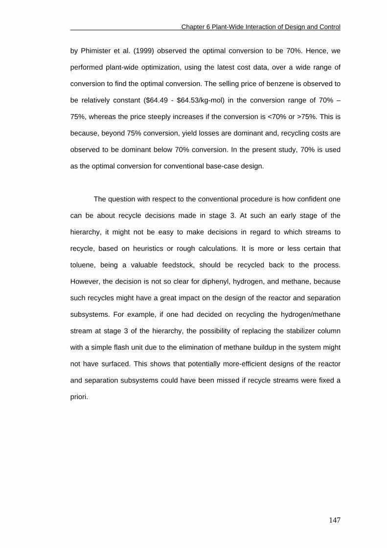
Chapter 6 Plant-Wide Interaction of Design and Control
by Phimister et al. (1999) observed the optimal conversion to be 70%. Hence, we
performed plant-wide optimization, using the latest cost data, over a wide range of
conversion to find the optimal conversion. The selling price of benzene is observed to
be relatively constant ($64.49 - $64.53/kg-mol) in the conversion range of 70% –
75%, whereas the price steeply increases if the conversion is <70% or >75%. This is
because, beyond 75% conversion, yield losses are dominant and, recycling costs are
observed to be dominant below 70% conversion. In the present study, 70% is used
as the optimal conversion for conventional base-case design.
The question with respect to the conventional procedure is how confident one
can be about recycle decisions made in stage 3. At such an early stage of the
hierarchy, it might not be easy to make decisions in regard to which streams to
recycle, based on heuristics or rough calculations. It is more or less certain that
toluene, being a valuable feedstock, should be recycled back to the process.
However, the decision is not so clear for diphenyl, hydrogen, and methane, because
such recycles might have a great impact on the design of the reactor and separation
subsystems. For example, if one had decided on recycling the hydrogen/methane
stream at stage 3 of the hierarchy, the possibility of replacing the stabilizer column
with a simple flash unit due to the elimination of methane buildup in the system might
not have surfaced. This shows that potentially more-efficient designs of the reactor
and separation subsystems could have been missed if recycle streams were fixed a
priori.
147
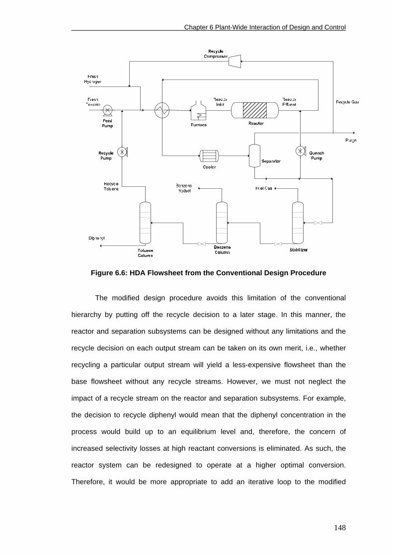
Chapter 6 Plant-Wide Interaction of Design and Control
Figure 6.6: HDA Flowsheet from the Conventional Design Procedure
The modified design procedure avoids this limitation of the conventional
hierarchy by putting off the recycle decision to a later stage. In this manner, the
reactor and separation subsystems can be designed without any limitations and the
recycle decision on each output stream can be taken on its own merit, i.e., whether
recycling a particular output stream will yield a less-expensive flowsheet than the
base flowsheet without any recycle streams. However, we must not neglect the
impact of a recycle stream on the reactor and separation subsystems. For example,
the decision to recycle diphenyl would mean that the diphenyl concentration in the
process would build up to an equilibrium level and, therefore, the concern of
increased selectivity losses at high reactant conversions is eliminated. As such, the
reactor system can be redesigned to operate at a higher optimal conversion.
Therefore, it would be more appropriate to add an iterative loop to the modified
148
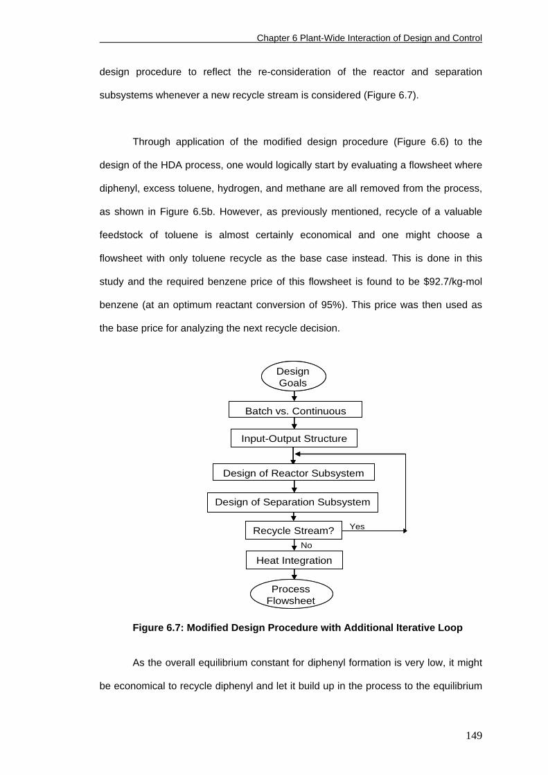
Chapter 6 Plant-Wide Interaction of Design and Control
design procedure to reflect the re-consideration of the reactor and separation
subsystems whenever a new recycle stream is considered (Figure 6.7).
Through application of the modified design procedure (Figure 6.6) to the
design of the HDA process, one would logically start by evaluating a flowsheet where
diphenyl, excess toluene, hydrogen, and methane are all removed from the process,
as shown in Figure 6.5b. However, as previously mentioned, recycle of a valuable
feedstock of toluene is almost certainly economical and one might choose a
flowsheet with only toluene recycle as the base case instead. This is done in this
study and the required benzene price of this flowsheet is found to be $92.7/kg-mol
benzene (at an optimum reactant conversion of 95%). This price was then used as
the base price for analyzing the next recycle decision.
Yes
No
Input-Output Structure
Design of Reactor Subsystem
Design of Separation Subsystem
Recycle Stream?
Heat Integration
Batch vs. Continuous
Design Goals
Process Flowsheet
Yes
No
Input-Output Structure
Design of Reactor Subsystem
Design of Separation Subsystem
Recycle Stream?
Heat Integration
Batch vs. Continuous
Design Goals
Process Flowsheet
Figure 6.7: Modified Design Procedure with Additional Iterative Loop
As the overall equilibrium constant for diphenyl formation is very low, it might
be economical to recycle diphenyl and let it build up in the process to the equilibrium
149
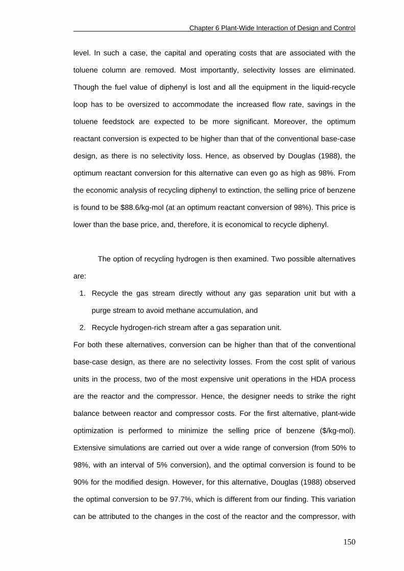
Chapter 6 Plant-Wide Interaction of Design and Control
level. In such a case, the capital and operating costs that are associated with the
toluene column are removed. Most importantly, selectivity losses are eliminated.
Though the fuel value of diphenyl is lost and all the equipment in the liquid-recycle
loop has to be oversized to accommodate the increased flow rate, savings in the
toluene feedstock are expected to be more significant. Moreover, the optimum
reactant conversion is expected to be higher than that of the conventional base-case
design, as there is no selectivity loss. Hence, as observed by Douglas (1988), the
optimum reactant conversion for this alternative can even go as high as 98%. From
the economic analysis of recycling diphenyl to extinction, the selling price of benzene
is found to be $88.6/kg-mol (at an optimum reactant conversion of 98%). This price is
lower than the base price, and, therefore, it is economical to recycle diphenyl.
The option of recycling hydrogen is then examined. Two possible alternatives
are:
1. Recycle the gas stream directly without any gas separation unit but with a
purge stream to avoid methane accumulation, and
2. Recycle hydrogen-rich stream after a gas separation unit.
For both these alternatives, conversion can be higher than that of the conventional
base-case design, as there are no selectivity losses. From the cost split of various
units in the process, two of the most expensive unit operations in the HDA process
are the reactor and the compressor. Hence, the designer needs to strike the right
balance between reactor and compressor costs. For the first alternative, plant-wide
optimization is performed to minimize the selling price of benzene ($/kg-mol).
Extensive simulations are carried out over a wide range of conversion (from 50% to
98%, with an interval of 5% conversion), and the optimal conversion is found to be
90% for the modified design. However, for this alternative, Douglas (1988) observed
the optimal conversion to be 97.7%, which is different from our finding. This variation
can be attributed to the changes in the cost of the reactor and the compressor, with
150
Chapter 6 Plant-Wide Interaction of Design and Control
them being the two most expensive equipments in the HDA process. Douglas’ cost
data were updated to the present-day values, for a fair comparison. About 27% hike
in reactor cost and about 23% reduction in the compressor cost are observed, which
obviously mean that a reactor with less volume and, hence, less conversion (and
more recycle) will be more economical, which is consistent with our finding. The
selling price of benzene for this alternative is observed to be $62.7/kg-mol at optimal
conversion (90%). This alternative is less expensive than the conventional base case
design ($64.5/kg-mol), despite the fact that it requires a larger reactor (in order to
achieve high conversion as there are no selectivity losses). The larger reactor
lessens the recycle flows and the controllability is expected to be better. However,
the number of recycling components here is more and may result in operational
problems. Hence, to gauge the operational benefits of this process design, rigorous
nonlinear dynamic simulations should be performed.
For the second alternative, membrane gas separation is considered, as it can
be economically competitive with conventional gas separation methods (such as
cryogenic distillation, absorption, and pressure-swing adsorption), especially when
the product purity requirements are not very high (Kao, 1987; Meindersma, 1991;
Scott, 1995). For processes, that require high-purity (> 99.9%) hydrogen, pressure
swing absorption can be cost-effective (Meindersma, 1991). However, for the HDA
process, the purity requirements on H2 are not very high, and, hence, membrane
separation can be a cost-effective alternative. In addition, the gas flow rate from flash
in the HDA process is low (<108 ft3/day), and, hence, membrane separation is the
most favorable option (Prasad et al., 1994). Several design issues that arise at this
stage are:
(1) Which membrane configuration – a simple, recycle-permeator or two-
membrane-type permeators, should be considered?
151
Chapter 6 Plant-Wide Interaction of Design and Control
(2) What should be the operating conditions of the membrane purification
unit? do the feed conditions (temperature and pressure) require preprocessing?
(3) What are the maximum attainable purity and recovery of hydrogen in the
permeate stream?
(4) Where should the membrane unit be placed - on the purge stream or the
flash vapor stream?
As the separation of hydrogen and methane is easy because of the higher
selectivity (values as high as 200 are reported by Zolandz and Fleming, 1992), a
simple membrane-permeator is considered in this study. As the gas feed to the
membrane is already available at high pressure (~ 445 psia), no further compression
is needed. As the gas feed to membrane is available at low temperature (100 oF),
polymeric membranes can be used without any difficulty in the operation.
Alternatively, one can consider inorganic membranes or mixed-matrix composite
membranes (with enhanced desirable characteristics). More than 95% purity and
recovery of H2 can be expected for H2/CH4 separation (Scott, 1995; Nakagawa,
1994).
The placement of the membrane unit introduces two more potential design
alternatives: place the membrane unit on the entire flash vapor stream or place it on
the purge stream. This placement has different economic and operational
implications on different sections of the plant (especially the reactor and compression
sections). The alternative with the membrane unit on the flash vapor stream has a
distinct feature – the methane content in the reactor is reduced to the smallest
possible value, which has both positive and negative effects. Owing to the relatively
lesser methane content in the reactor section, the required reactor volume would be
less and, hence, reactor is less expensive. On the other hand, there is a greater
possibility that the reactor outlet temperature would exceed the maximum allowable
152
Chapter 6 Plant-Wide Interaction of Design and Control
value due to the reduced methane content in the reactor coupled with the fact that
the optimal conversion is relatively high. Recall that methane in the reactor serves as
thermal sink to keep the outlet temperature well below the constrained value, as in
other alternatives. Consequently, the reactor section has to be modified accordingly,
which will be discussed later. Similarly there are differences in the compression
section of both the alternatives. Compression costs in the first alternative, i.e., the
process with the membrane unit on the flash vapor stream, would be higher as all the
relatively high-purity hydrogen (i.e., membrane permeate) has to be compressed to
the reactor conditions from very low pressures. Although the second alternative, i.e.,
the process with the membrane unit on the purge stream, requires two compressors
– one to compress the membrane permeate and the other to compress the gas
recycle stream (which is already at relatively high pressures), the overall
compression cost is expected to be less, compared to the first alternative as the
amount of membrane permeate is relatively less. However, the aforementioned
merits of the second alternative are dependent on the purge ratio (i.e., what fraction
of flash vapor stream is taken out as purge). Hence, both alternatives are analyzed
further.
The alternative with the membrane unit placed on the flash vapor is
considered first, and brief description of the membrane unit† is given as follows. The
feed to the membrane is at 445 psia and 100 oF. The CH4-rich retentate is assumed
to be leaving at the same temperature and with a small pressure drop (5 psia), and, it
can be used a fuel gas. H2-rich permeate is assumed to be leaving at a much lower
pressure (i.e., 45 psia in order to provide a good driving force for separation) and a
temperature (95 oF) slightly lower than the feed temperature (100 oF). Based on the
Hydrogen Production Facilities Plant Performance and Cost Comparisons Final
† Due to the unavailability of the membrane unit in HYSYS, an extension from the Aspentech support website is used here to simulate the membrane unit.
153
Chapter 6 Plant-Wide Interaction of Design and Control
Report published in March 2002 by Parsons Infrastructure and Technology Group
Inc. (http://www.fischer-tropsch.org/DOE/DOE_reports/40465_fr/40465_fr_toc.htm,
accessed in April, 2006), a value of 0.1 std cc/min/cm2/cm Hg was used as the
hydrogen flux through the membrane. Zolandz and Fleming (1992) suggested an
optimal selectivity of 110 for H2-CH4 separation, and, hence, it is used in this study.
The required membrane area is estimated to be 186 m2 to achieve 98% pure
hydrogen and 98% recovery of hydrogen in permeate. A spiral-wound module, which
is relatively less expensive than a tubular module, is considered; alternatively,
hollow-fiber modules can be considered, which are much cheaper but they suffer
from fouling. The cost of spiral-wound modules can vary between US$10/m2 and
US$100/m2 (Baker, 2002); therefore, an average value of US$55/m2 is assumed.
With these specifications, the membrane cost is only 0.23% of the overall capital
cost, and, hence, any uncertainty in the membrane information will not affect overall
conclusions that will be deduced. Although the membrane operation is observed to
be relatively inexpensive, one of the problems with membrane operation is that the
permeate pressure (usually close to atmospheric pressure) will be well below the
feed pressure. Hence, in the HDA process, the permeate compressor is observed to
be expensive (almost one-third of the total capital cost), and the operating cost is
also significant.
In the conventional base-case design for the HDA process, the excessive
methane content in the reactor serves as a heat-sink to maintain the reactor outlet
temperature well below the upper limit (1300 0F) to avoid cracking, although the
reactor is adiabatic. However, in the modified HDA process with the membrane unit
on the flash vapor stream, the amount of methane within the reactor is significantly
less as most of the methane is removed by the membrane unit. Also, as there are no
selectivity losses, the optimal conversion for the process with the membrane unit is
expected to be higher than that of the conventional HDA process (70-75%). Hence,
154
Chapter 6 Plant-Wide Interaction of Design and Control
more energy will be released in the reactor and the outlet temperature of an adiabatic
reactor is unlikely to be within the upper limit. Two possible alternatives are (i) a
single nonadiabatic reactor, and (ii) two adiabatic reactors in series with toluene feed-
split and an inter-stage heater (Figure 6.8). As mentioned previously, the main
problem with the alternatives having a membrane separator is that it requires an
expensive compressor, which should be compensated by savings that are introduced
by membrane separator (i.e., by reducing reactor cost and saving valuable
feedstock). The selling price of benzene is found to be $60.9/kgmol and $63.2/kgmol
(at an optimum reactant conversion of 98%) for the alternatives with a single
nonadiabatic reactor and two adiabatic reactors respectively. For the latter
alternative, toluene is equally split between the two reactors, which are designed to
give equal conversion; this implies that the reactors are in parallel with respect to
toluene flow and in series with respect to hydrogen flow (Figure 6.8).
Next, the alternative of the membrane unit on the purge stream is considered.
As discussed previously, this alternative has significant methane in the reactor, which
acts as a thermal sink, and, hence, a single adiabatic reactor is sufficient. As
expected, the required membrane area is now less as the amount of membrane feed
is relatively less. Of all the alternatives, this alternative has more number of recycles
and poses more convergence difficulties in steady-state. Hence, recycle blocks are
placed judiciously to improve the computational efficiency for optimization studies. In
general, the higher the conversion, the more economical is the process, and, hence,
the optimum conversion is found to be 98%. Unlike the two alternatives that have the
membrane unit on the flash vapor stream, there is one more design variable, namely,
purge ratio (i.e., the fraction of flash vapor flow that is purged out and sent to the
membrane). Therefore, optimization is carried out with the purge ratio as the decision
variable. Initially, profitability of the process increases as the purge ratio increases.
However, beyond a purge ratio of 0.25, the loss of hydrogen in the purge becomes
155
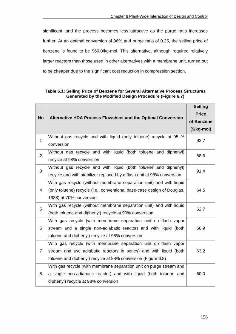
Chapter 6 Plant-Wide Interaction of Design and Control
significant, and the process becomes less attractive as the purge ratio increases
further. At an optimal conversion of 98% and purge ratio of 0.25, the selling price of
benzene is found to be $60.0/kg-mol. This alternative, although required relatively
larger reactors than those used in other alternatives with a membrane unit, turned out
to be cheaper due to the significant cost reduction in compression section.
Table 6.1: Selling Price of Benzene for Several Alternative Process Structures Generated by the Modified Design Procedure (Figure 6.7)
No Alternative HDA Process Flowsheet and the Optimal Conversion
Selling Price
of Benzene($/kg-mol)
1 Without gas recycle and with liquid (only toluene) recycle at 95 %
conversion 92.7
2 Without gas recycle and with liquid (both toluene and diphenyl)
recycle at 98% conversion 88.6
3 Without gas recycle and with liquid (both toluene and diphenyl)
recycle and with stabilizer replaced by a flash unit at 98% conversion 91.4
4
With gas recycle (without membrane separation unit) and with liquid
(only toluene) recycle (i.e., conventional base-case design of Douglas,
1988) at 70% conversion
64.5
5 With gas recycle (without membrane separation unit) and with liquid
(both toluene and diphenyl) recycle at 90% conversion 62.7
6
With gas recycle (with membrane separation unit on flash vapor
stream and a single non-adiabatic reactor) and with liquid (both
toluene and diphenyl) recycle at 98% conversion
60.9
7
With gas recycle (with membrane separation unit on flash vapor
stream and two adiabatic reactors in series) and with liquid (both
toluene and diphenyl) recycle at 98% conversion (Figure 6.8)
63.2
8
With gas recycle (with membrane separation unit on purge stream and
a single non-adiabatic reactor) and with liquid (both toluene and
diphenyl) recycle at 98% conversion
60.0
156
Chapter 6 Plant-Wide Interaction of Design and Control
Overall, the alternatives with membrane gas separation unit are more
economical (Table 6.1); of them, alternative 8 is the most economical. This result is
consistent with that of Kocis and Grossmann (Kocis and Grossmann, 1989) and Goel
et al., (2002) who have optimized the HDA process flowsheet using MINLP.
However, in their studies, process design selection was purely based on steady-state
analysis; dynamic implications were not considered. Alternative 6 is the next-best
alternative followed by alternatives 5, 7, and 4. Although Douglas (1988) studied
several of these alternatives, alternatives involving membranes (especially
alternatives 6 and 7) have not been studied, perhaps because of the unavailability of
design and cost data for membranes at that time. Alternative 3, though not
economical, was neither explored nor possible to be explored by the conventional
design procedure. The alternatives without gas and/or liquid recycle are more
expensive, because the feed stocks cost contribution towards overall cost is high
(Figure 6.8).
To conclude, the modified design procedure, while retaining all the benefits of
the conventional design procedure, allows the designer to explore more alternatives
in a systematic way. One major modification in the modified design procedure is to
consider recycles towards the end of the design procedure, based on their own
economical merit. This suggestion is not only beneficial from the point of steady-state
design but it is also useful for efficient control system design, as discussed in the
next section. As PWC analysis is computationally very intensive and requires careful
scrutiny of many transients, only the most promising alternatives are considered in
the subsequent section. This is justifiable as one would not want to consider very
uneconomical processes, irrespective of how well they can be controlled. At this
stage, the designer has to choose the alternatives that are worth considering for
dynamic analysis. In case of HDA process, alternatives 4 to 8 are more economical,
and, so they are forwarded to the next (i.e., control) stage.
157
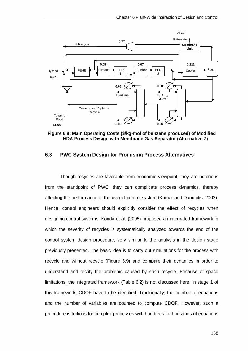
Chapter 6 Plant-Wide Interaction of Design and Control
-0.02
-1.42
0.11
0.06
0.05
0.001
0.2110.08
0.77
44.55
6.27
H2, CH4Benzene
RetentateH2Recycle
Toluene and DiphenylRecycle
TolueneFeed
H2 feed FlashFEHE Furnace PFR1
Cooler
0.07Furnace PFR
2
MembraneUnit
-0.02
-1.42
0.11
0.06
0.05
0.001
0.2110.08
0.77
44.55
6.27
H2, CH4Benzene
RetentateH2Recycle
Toluene and DiphenylRecycle
TolueneFeed
H2 feed FlashFEHE Furnace PFR1
Cooler
0.07Furnace PFR
2
MembraneUnit
Figure 6.8: Main Operating Costs ($/kg-mol of benzene produced) of Modified
HDA Process Design with Membrane Gas Separator (Alternative 7)
6.3 PWC System Design for Promising Process Alternatives
Though recycles are favorable from economic viewpoint, they are notorious
from the standpoint of PWC; they can complicate process dynamics, thereby
affecting the performance of the overall control system (Kumar and Daoutidis, 2002).
Hence, control engineers should explicitly consider the effect of recycles when
designing control systems. Konda et al. (2005) proposed an integrated framework in
which the severity of recycles is systematically analyzed towards the end of the
control system design procedure, very similar to the analysis in the design stage
previously presented. The basic idea is to carry out simulations for the process with
recycle and without recycle (Figure 6.9) and compare their dynamics in order to
understand and rectify the problems caused by each recycle. Because of space
limitations, the integrated framework (Table 6.2) is not discussed here. In stage 1 of
this framework, CDOF have to be identified. Traditionally, the number of equations
and the number of variables are counted to compute CDOF. However, such a
procedure is tedious for complex processes with hundreds to thousands of equations
158
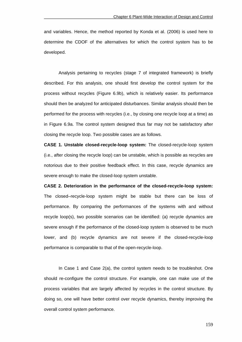
Chapter 6 Plant-Wide Interaction of Design and Control
and variables. Hence, the method reported by Konda et al. (2006) is used here to
determine the CDOF of the alternatives for which the control system has to be
developed.
Analysis pertaining to recycles (stage 7 of integrated framework) is briefly
described. For this analysis, one should first develop the control system for the
process without recycles (Figure 6.9b), which is relatively easier. Its performance
should then be analyzed for anticipated disturbances. Similar analysis should then be
performed for the process with recycles (i.e., by closing one recycle loop at a time) as
in Figure 6.9a. The control system designed thus far may not be satisfactory after
closing the recycle loop. Two possible cases are as follows.
CASE 1. Unstable closed-recycle-loop system: The closed-recycle-loop system
(i.e., after closing the recycle loop) can be unstable, which is possible as recycles are
notorious due to their positive feedback effect. In this case, recycle dynamics are
severe enough to make the closed-loop system unstable.
CASE 2. Deterioration in the performance of the closed-recycle-loop system:
The closed–recycle-loop system might be stable but there can be loss of
performance. By comparing the performances of the systems with and without
recycle loop(s), two possible scenarios can be identified: (a) recycle dynamics are
severe enough if the performance of the closed-loop system is observed to be much
lower, and (b) recycle dynamics are not severe if the closed-recycle-loop
performance is comparable to that of the open-recycle-loop.
In Case 1 and Case 2(a), the control system needs to be troubleshot. One
should re-configure the control structure. For example, one can make use of the
process variables that are largely affected by recycles in the control structure. By
doing so, one will have better control over recycle dynamics, thereby improving the
overall control system performance.
159
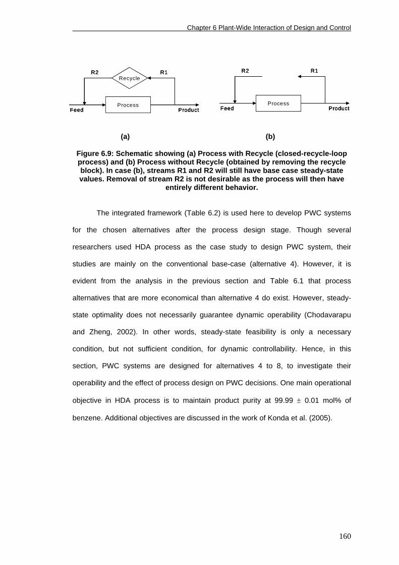
Chapter 6 Plant-Wide Interaction of Design and Control
Process
Recycle
Feed Product
R1R2
ProcessFeed Product
R1R2
Process
Recycle
Feed Product
R1R2
Process
Recycle
Feed Product
R1R2
ProcessFeed Product
R1R2
ProcessFeed Product
R1R2
(a) (b)
Figure 6.9: Schematic showing (a) Process with Recycle (closed-recycle-loop process) and (b) Process without Recycle (obtained by removing the recycle block). In case (b), streams R1 and R2 will still have base case steady-state values. Removal of stream R2 is not desirable as the process will then have
entirely different behavior.
The integrated framework (Table 6.2) is used here to develop PWC systems
for the chosen alternatives after the process design stage. Though several
researchers used HDA process as the case study to design PWC system, their
studies are mainly on the conventional base-case (alternative 4). However, it is
evident from the analysis in the previous section and Table 6.1 that process
alternatives that are more economical than alternative 4 do exist. However, steady-
state optimality does not necessarily guarantee dynamic operability (Chodavarapu
and Zheng, 2002). In other words, steady-state feasibility is only a necessary
condition, but not sufficient condition, for dynamic controllability. Hence, in this
section, PWC systems are designed for alternatives 4 to 8, to investigate their
operability and the effect of process design on PWC decisions. One main operational
objective in HDA process is to maintain product purity at 99.99 ± 0.01 mol% of
benzene. Additional objectives are discussed in the work of Konda et al. (2005).
160
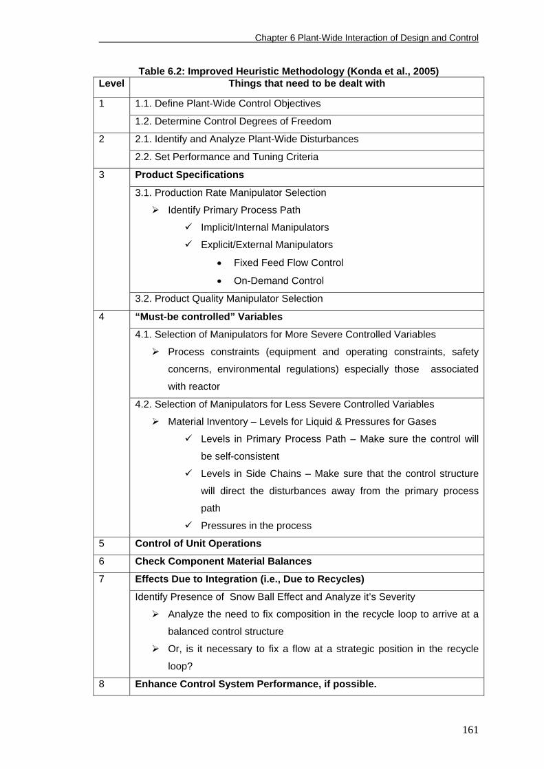
Chapter 6 Plant-Wide Interaction of Design and Control
Table 6.2: Improved Heuristic Methodology (Konda et al., 2005) Level Things that need to be dealt with
1.1. Define Plant-Wide Control Objectives 1
1.2. Determine Control Degrees of Freedom
2.1. Identify and Analyze Plant-Wide Disturbances 2
2.2. Set Performance and Tuning Criteria
Product Specifications
3.1. Production Rate Manipulator Selection
Identify Primary Process Path
Implicit/Internal Manipulators
Explicit/External Manipulators
• Fixed Feed Flow Control
• On-Demand Control
3
3.2. Product Quality Manipulator Selection
“Must-be controlled” Variables
4.1. Selection of Manipulators for More Severe Controlled Variables
Process constraints (equipment and operating constraints, safety
concerns, environmental regulations) especially those associated
with reactor
4
4.2. Selection of Manipulators for Less Severe Controlled Variables
Material Inventory – Levels for Liquid & Pressures for Gases
Levels in Primary Process Path – Make sure the control will
be self-consistent
Levels in Side Chains – Make sure that the control structure
will direct the disturbances away from the primary process
path
Pressures in the process
5 Control of Unit Operations
6 Check Component Material Balances
Effects Due to Integration (i.e., Due to Recycles) 7
Identify Presence of Snow Ball Effect and Analyze it’s Severity
Analyze the need to fix composition in the recycle loop to arrive at a
balanced control structure
Or, is it necessary to fix a flow at a strategic position in the recycle
loop?
8 Enhance Control System Performance, if possible.
161
Chapter 6 Plant-Wide Interaction of Design and Control
6.3.1 Dynamic Performance Analysis
Before describing control system design for alternatives 4 to 8, measures of
its performance analysis are first discussed as these are needed for choosing control
design options. Luyben and co-workers (Elliott and Luyben, 1995, 1996 & 1997)
proposed capacity-based approach to measure the dynamic performance of
alternative designs by computing the loss in capacity due to off-spec production; the
measure is thus related to product quality regulation. Though capacity-based
approach is a useful and practical measure, it cannot be applied in all situations. For
example, according to this approach, the off-spec product is assumed to be
disposed. However, it may be economical to recycle it as the raw materials are
usually expensive. Otherwise, yield-losses will be there and additional costs due to
disposal of the off-spec product may render the process economically unattractive.
Though it is possible to implement this feature in the capacity-based approach, it
cannot be generalized. It may not be desirable to recycle the overpurified off-spec
product (although the underpurified off-spec product need to be recycled) as it
unnecessarily incurs additional costs. Even if the off-spec product has to be recycled,
the recycling location and reprocessing cost will be process-specific. If the off-spec
product is due to light impurities, it has to be recycled back to the light-component
(impurity) purification section; otherwise, it has to be processed through the heavy-
component (impurity) purification section. At times, the off-spec product can not be
recycled due to capacity limitations (Zheng and Mahajanam, 1999; Mahajanam and
Zheng, 2002), but it has to be stored (for future processing), which incurs additional
inventory costs. Thus, the reprocessing cost of the off-spec product will be different in
each of these cases, and no generally accepted procedures are available to estimate
it. One can assume some cost, but the results will be dependent on this assumed
value.
162
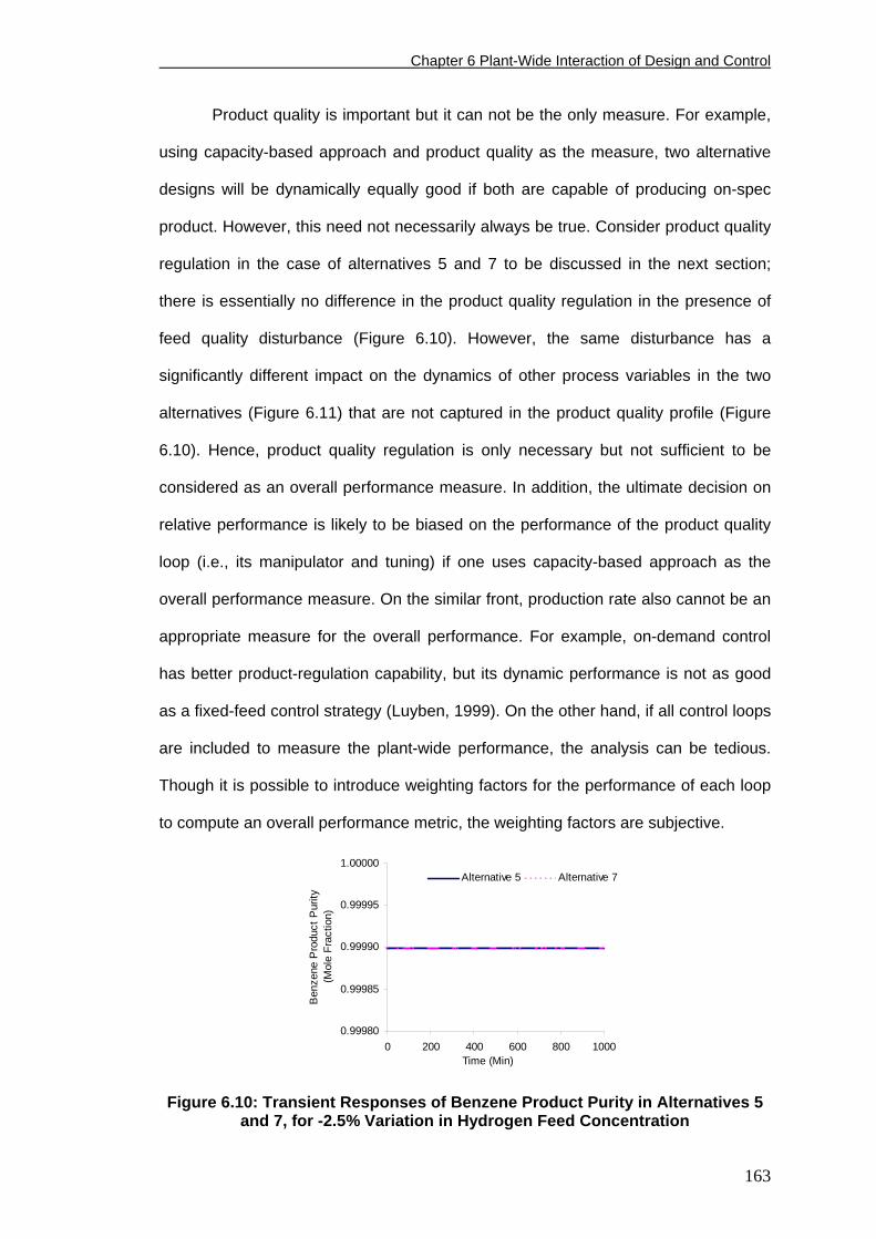
Chapter 6 Plant-Wide Interaction of Design and Control
Product quality is important but it can not be the only measure. For example,
using capacity-based approach and product quality as the measure, two alternative
designs will be dynamically equally good if both are capable of producing on-spec
product. However, this need not necessarily always be true. Consider product quality
regulation in the case of alternatives 5 and 7 to be discussed in the next section;
there is essentially no difference in the product quality regulation in the presence of
feed quality disturbance (Figure 6.10). However, the same disturbance has a
significantly different impact on the dynamics of other process variables in the two
alternatives (Figure 6.11) that are not captured in the product quality profile (Figure
6.10). Hence, product quality regulation is only necessary but not sufficient to be
considered as an overall performance measure. In addition, the ultimate decision on
relative performance is likely to be biased on the performance of the product quality
loop (i.e., its manipulator and tuning) if one uses capacity-based approach as the
overall performance measure. On the similar front, production rate also cannot be an
appropriate measure for the overall performance. For example, on-demand control
has better product-regulation capability, but its dynamic performance is not as good
as a fixed-feed control strategy (Luyben, 1999). On the other hand, if all control loops
are included to measure the plant-wide performance, the analysis can be tedious.
Though it is possible to introduce weighting factors for the performance of each loop
to compute an overall performance metric, the weighting factors are subjective.
0.99980
0.99985
0.99990
0.99995
1.00000
0 200 400 600 800 1000Time (Min)
Ben
zene
Pro
duct
Pur
ity
(Mol
e Fr
actio
n)
Alternative 5 Alternative 7
Figure 6.10: Transient Responses of Benzene Product Purity in Alternatives 5 and 7, for -2.5% Variation in Hydrogen Feed Concentration
163
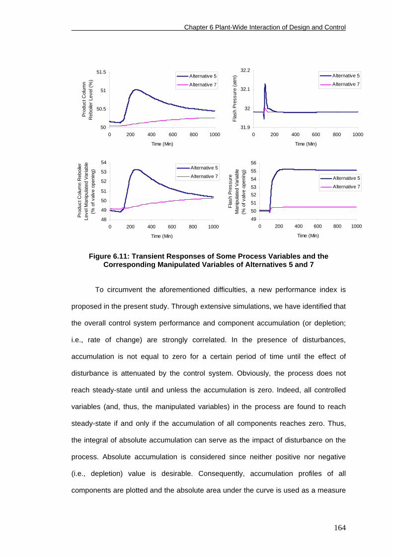
Chapter 6 Plant-Wide Interaction of Design and Control
50
50.5
51
51.5
0 200 400 600 800 1000
Time (Min)
Prod
uct C
olum
n R
eboi
ler L
evel
(%)
Alternative 5
Alternative 7
48
49
50
51
52
53
54
0 200 400 600 800 1000
Time (Min)
Prod
uct C
olum
n R
eboi
ler
Leve
l Man
ipul
ated
Var
iabl
e (%
of v
alve
ope
ning
) Alternative 5
Alternative 7
31.9
32
32.1
32.2
0 200 400 600 800 1000
Time (Min)
Flas
h Pr
essu
re (a
tm) Alternative 5
Alternative 7
4950515253545556
0 200 400 600 800 1000
Time (Min)Fl
ash
Pres
sure
M
anip
ulat
ed V
aria
ble
(% o
f val
ve o
peni
ng)
Alternative 5
Alternative 7
Figure 6.11: Transient Responses of Some Process Variables and the Corresponding Manipulated Variables of Alternatives 5 and 7
To circumvent the aforementioned difficulties, a new performance index is
proposed in the present study. Through extensive simulations, we have identified that
the overall control system performance and component accumulation (or depletion;
i.e., rate of change) are strongly correlated. In the presence of disturbances,
accumulation is not equal to zero for a certain period of time until the effect of
disturbance is attenuated by the control system. Obviously, the process does not
reach steady-state until and unless the accumulation is zero. Indeed, all controlled
variables (and, thus, the manipulated variables) in the process are found to reach
steady-state if and only if the accumulation of all components reaches zero. Thus,
the integral of absolute accumulation can serve as the impact of disturbance on the
process. Absolute accumulation is considered since neither positive nor negative
(i.e., depletion) value is desirable. Consequently, accumulation profiles of all
components are plotted and the absolute area under the curve is used as a measure
164
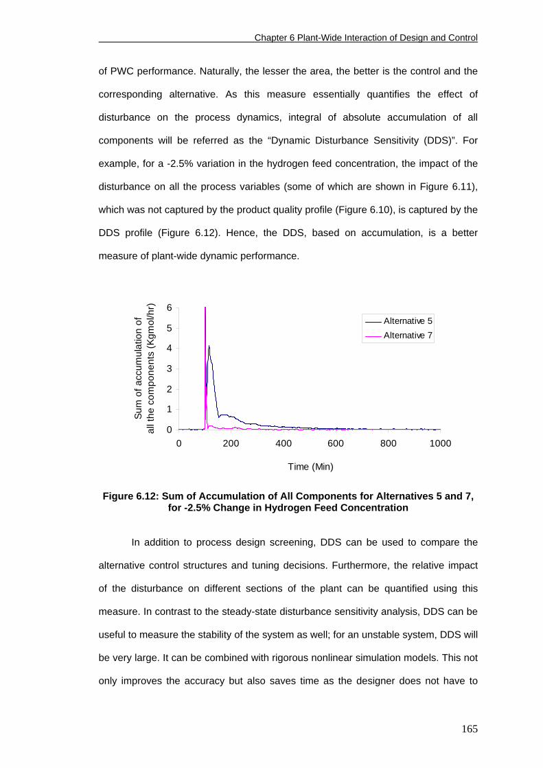
Chapter 6 Plant-Wide Interaction of Design and Control
of PWC performance. Naturally, the lesser the area, the better is the control and the
corresponding alternative. As this measure essentially quantifies the effect of
disturbance on the process dynamics, integral of absolute accumulation of all
components will be referred as the “Dynamic Disturbance Sensitivity (DDS)”. For
example, for a -2.5% variation in the hydrogen feed concentration, the impact of the
disturbance on all the process variables (some of which are shown in Figure 6.11),
which was not captured by the product quality profile (Figure 6.10), is captured by the
DDS profile (Figure 6.12). Hence, the DDS, based on accumulation, is a better
measure of plant-wide dynamic performance.
0
1
2
3
4
5
6
0 200 400 600 800 1000
Time (Min)
Sum
of a
ccum
ulat
ion
of
all t
he c
ompo
nent
s (K
gmol
/hr)
Alternative 5Alternative 7
Figure 6.12: Sum of Accumulation of All Components for Alternatives 5 and 7, for -2.5% Change in Hydrogen Feed Concentration
In addition to process design screening, DDS can be used to compare the
alternative control structures and tuning decisions. Furthermore, the relative impact
of the disturbance on different sections of the plant can be quantified using this
measure. In contrast to the steady-state disturbance sensitivity analysis, DDS can be
useful to measure the stability of the system as well; for an unstable system, DDS will
be very large. It can be combined with rigorous nonlinear simulation models. This not
only improves the accuracy but also saves time as the designer does not have to
165
Chapter 6 Plant-Wide Interaction of Design and Control
linearize the nonlinear models for linear model-based controllability indexes to
analyze the performance. DDS is equally applicable to performance analysis for set-
point changes. Furthermore, DDS is very useful to assess the dynamics of the
process (such as overall time constant) without having to examine all the process
variables to identify the slowest-responding one, which, in turn, is dependent on
several other factors (e.g., the type of disturbance). In the case of complex processes
where large number of alternatives is possible, DDS can quickly screen the
alternative control structures and process designs, based on their dynamic
performance. In the following sections, it is used to assess the dynamic performance
of process design and control alternatives in the presence of several anticipated
disturbances. Controller design and tuning is done in the same way as was done in
Chapter 5. See section 5.4.2 and Appendix C for more details on controller design
and tuning.
6.3.2 PWC System Design for Alternative 4
The PWC system for the conventional HDA process has recently been
designed by Konda et al. (2005) and is presented in Chapter 3; therefore, it is not
discussed here extensively. They carried out the analysis without the recycles until
step 6 and control decisions are taken accordingly. The resulting control structure
after step 6 is summarized in Table C.1 (Appendix C). Thus far, the analysis is
performed without gas and liquid recycles (i.e., by tearing both the gas and liquid
recycle streams). All the control decisions taken so far lead to a control system that is
stable even with both of the recycles. However, as shown in the following analysis, a
better control system is generated by systematically analyzing the effect of recycles
on the overall plant dynamics.
166
Chapter 6 Plant-Wide Interaction of Design and Control
Effect of Gas Recycle on Overall Plant Dynamics: The closed-loop dynamic
simulation is run with each of the expected disturbances for the HDA process with and
without gas recycle, and the effect of gas recycle on the overall plant dynamics is
observed to be negligible when compared to that of liquid recycle. Hence, further
analysis is carried out based solely on the impact of liquid recycle on the overall
dynamics. The gas recycle contains a purge stream to avoid accumulation of methane
in the process; hence, a composition controller is needed to make the methane
inventory in the process self-regulating. The composition of the purge stream is
controlled by manipulating recycle gas flow. Simulations showed that this composition
does not vary much, even in the presence of disturbances. Therefore, one can replace
the purge composition controller with a ratio controller (i.e., to maintain the purge flow
as a fraction of gas flow) to avoid the use of expensive composition analyzer. In the
present study, a composition controller is assumed in the subsequent analysis for
alternative 4.
Effect of Liquid Recycle on Overall Plant Dynamics: The two processes,
one with liquid recycle and the other without liquid recycle (Figure 6.9), are initially
perturbed with two of the most significant and commonly encountered disturbances
(i.e., -5% and -25% variation in the toluene feed flow rate). The responses of process
variables such as conversion are rated as acceptable or not acceptable, based on
how close/far they are to the optimal steady-state values in the presence of
disturbances (Table 6.3). In Tables 6.3 and 6.4, variation in conversion and the
overall process settling time (taking into account all process variables) are given for a
-5% variation in toluene feed flow rate where as the equipment constraints are given
for the worst-case disturbance of -25% variation in the toluene feed flow rate. As can
be seen from the summary in Table 6.3, the liquid recycle dynamics are severe
enough to deteriorate the control system performance significantly, indicating the
need for a better control structure. The responses of process variables are then
167
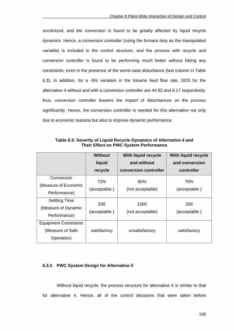
Chapter 6 Plant-Wide Interaction of Design and Control
scrutinized, and the conversion is found to be greatly affected by liquid recycle
dynamics. Hence, a conversion controller (using the furnace duty as the manipulated
variable) is included in the control structure, and the process with recycle and
conversion controller is found to be performing much better without hitting any
constraints, even in the presence of the worst-case disturbance (last column in Table
6.3). In addition, for a -5% variation in the toluene feed flow rate, DDS for the
alternative 4 without and with a conversion controller are 44.92 and 8.17 respectively;
thus, conversion controller lessens the impact of disturbances on the process
significantly. Hence, the conversion controller is needed for this alternative not only
due to economic reasons but also to improve dynamic performance.
Table 6.3: Severity of Liquid Recycle Dynamics of Alternative 4 and Their Effect on PWC System Performance
Without
liquid recycle
With liquid recycle and without
conversion controller
With liquid recycle and conversion
controller
Conversion
(Measure of Economic
Performance)
72%
(acceptable )
80%
(not acceptable)
70%
(acceptable )
Settling Time
(Measure of Dynamic
Performance)
200
(acceptable ) 1000
(not acceptable)
200
(acceptable )
Equipment Constraints
(Measure of Safe
Operation)
satisfactory unsatisfactory satisfactory
6.3.3 PWC System Design for Alternative 5
Without liquid recycle, the process structure for alternative 5 is similar to that
for alternative 4. Hence, all of the control decisions that were taken before
168
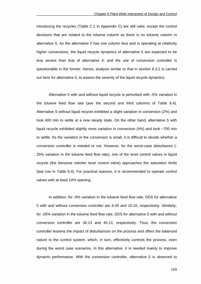
Chapter 6 Plant-Wide Interaction of Design and Control
introducing the recycles (Table C.1 in Appendix C) are still valid, except the control
decisions that are related to the toluene column as there is no toluene column in
alternative 5. As the alternative 5 has one column less and is operating at relatively
higher conversions, the liquid recycle dynamics of alternative 5 are expected to be
less severe than that of alternative 4, and the use of conversion controller is
questionable in the former. Hence, analysis similar to that in section 6.3.2 is carried
out here for alternative 5, to assess the severity of the liquid recycle dynamics.
Alternative 5 with and without liquid recycle is perturbed with -5% variation in
the toluene feed flow rate (see the second and third columns of Table 6.4).
Alternative 5 without liquid recycle exhibited a slight variation in conversion (2%) and
took 400 min to settle at a new steady state. On the other hand, alternative 5 with
liquid recycle exhibited slightly more variation in conversion (4%) and took ~700 min
to settle. As the variation in the conversion is small, it is difficult to decide whether a
conversion controller is needed or not. However, for the worst-case disturbance (-
25% variation in the toluene feed flow rate), one of the level control valves in liquid
recycle (the benzene reboiler level control valve) approaches the saturation limits
(last row in Table 6.4). For practical reasons, it is recommended to operate control
valves with at least 10% opening.
In addition, for -5% variation in the toluene feed flow rate, DDS for alternative
5 with and without conversion controller are 6.45 and 10.10, respectively. Similarly,
for -25% variation in the toluene feed flow rate, DDS for alternative 5 with and without
conversion controller are 30.13 and 40.13, respectively. Thus, the conversion
controller lessens the impact of disturbances on the process and offers the balanced
nature to the control system, which, in turn, effectively controls the process, even
during the worst case scenarios. In this alternative, it is needed mainly to improve
dynamic performance. With the conversion controller, alternative 5 is observed to
169
Chapter 6 Plant-Wide Interaction of Design and Control
give satisfactory performance (see the fourth column of Table 6.4) for feed flow rate
variations. In addition, several other disturbances are tried and the results are
analyzed in section 6.4.
Table 6.4: Severity of Liquid Recycle Dynamics of Alternative 5 and Their Effect on PWC System Performance
Without liquid
recycle With liquid recycle
and without conversion controller
With liquid recycle and conversion
controller
Conversion
(Measure of Economic
Performance)
92%
(acceptable ) 94%
(acceptable)
90%
(acceptable)
Settling Time
(Measure of Dynamic
Performance)
400
(acceptable) 700
(not acceptable)
150
(acceptable)
Equipment Constraints
(Measure of
Safe Operation)
satisfactory unsatisfactory satisfactory
6.3.4 PWC System Design for Alternative 6
As discussed in the previous section, for the process without gas and liquid
recycles, the control decisions taken up to stage 6 of the integrated framework (Table
C.1 in Appendix C) remain the same. Step 7 involves the introduction of gas and
liquid recycles, one by one, to examine their effects on the overall plant dynamics,
which are discussed in this section. Introducing gas recycle involves implementation
of the membrane control system, which is discussed below.
170
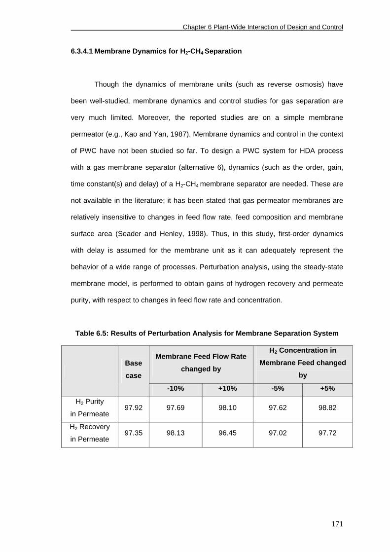
Chapter 6 Plant-Wide Interaction of Design and Control
6.3.4.1 Membrane Dynamics for H2-CH4 Separation
Though the dynamics of membrane units (such as reverse osmosis) have
been well-studied, membrane dynamics and control studies for gas separation are
very much limited. Moreover, the reported studies are on a simple membrane
permeator (e.g., Kao and Yan, 1987). Membrane dynamics and control in the context
of PWC have not been studied so far. To design a PWC system for HDA process
with a gas membrane separator (alternative 6), dynamics (such as the order, gain,
time constant(s) and delay) of a H2-CH4 membrane separator are needed. These are
not available in the literature; it has been stated that gas permeator membranes are
relatively insensitive to changes in feed flow rate, feed composition and membrane
surface area (Seader and Henley, 1998). Thus, in this study, first-order dynamics
with delay is assumed for the membrane unit as it can adequately represent the
behavior of a wide range of processes. Perturbation analysis, using the steady-state
membrane model, is performed to obtain gains of hydrogen recovery and permeate
purity, with respect to changes in feed flow rate and concentration.
Table 6.5: Results of Perturbation Analysis for Membrane Separation System
Membrane Feed Flow Rate changed by
H2 Concentration in Membrane Feed changed
by
Base case
-10% +10% -5% +5%
H2 Purity
in Permeate 97.92 97.69 98.10 97.62 98.82
H2 Recovery
in Permeate 97.35 98.13 96.45 97.02 97.72
171
Chapter 6 Plant-Wide Interaction of Design and Control
The recovery and purity of H2 in permeate are relatively insensitive to the expected
disturbances in the membrane feed flow rate and concentration (Table 6.5). Hence,
the dynamics of concentration can be ignored and, therefore, H2 concentration in
permeate is assumed to be constant at 98%. However, though the H2 recovery in
permeate is practically constant, the permeate flow rate changes with the membrane
feed flow rate and, therefore, its dynamics have to be considered. Because the
dynamic membrane unit operation is not available in HYSYS, a transfer function is
introduced to simulate the dynamics due to changes in membrane feed flow rate. The
transfer function is built between the component molar flow rate of hydrogen in flash
vapor to the molar flow rate of permeate, and the gain is specified as 1, since any
change in input causes an equal change in the output. This specification, together
with the permeate purity specification (98% H2), provides 98% recovery of H2, which
is close enough to the desired steady-state value (Table 6.5). Time constant and
delay are not yet known; in reality, they depend on several issues: the type of
membrane module (spiral-wound or hollow fiber membrane), the type of membrane
(dense or porous, glassy or rubbery), the type of membrane material (polymer,
inorganic or composite), the membrane configuration (simple or recycle), and the
permeabilities of the components involved. Because of the lack of this information in
the literature, a conservative estimate of 10 min for time constant is assumed, and
delay is taken as 10% of the time constant. To account for any uncertainty in these
values, several simulations are run with time constants of 1, 5 and 20 min to see its
effect on decisions being taken; however, these differences in the overall process
dynamics are observed to be insignificant. As the flash temperature is controlled, the
temperature of the feed (and that of permeate) are expected to be relatively constant.
Hence, the temperature dynamics are ignored. The membrane downstream pressure
varies with the permeate flow; a valve is used to simulate the downstream pressure
dynamics with flow variations.
172
Chapter 6 Plant-Wide Interaction of Design and Control
6.3.4.2 Control System Design for Gas Membrane
Usually, the membrane feed temperature and pressure are maintained at
constant values. However, as the flash temperature is already controlled, there is no
need for any additional control over the membrane feed temperature. Though the
flash pressure is also controlled using the valve on the flash vapor stream, there can
be some fluctuations in the membrane feed pressure in the range of 20-30 psia.
However, within this range of fluctuations, the membrane performance is not affected
much and, hence, no control loop is needed for membrane feed pressure regulation.
After introducing membrane dynamics and control system, analysis similar to
that carried out in sections 6.3.2 and 6.3.3, is done to characterize the severity of the
gas and liquid recycle dynamics. It is found that recycle dynamics are not severe as
the process is operating at very high conversion (~98%). Therefore, conversion
controller is not required for alternative 6.
6.3.5 PWC System Design for Alternative 7
Process structures of alternatives 6 and 7 are very similar; the only difference
is that alternative 6 has one nonadiabatic reactor and alternative 7 has two adiabatic
reactors in series (Figure 6.13; detailed separation section of alternative 7 is shown
in Figure 6.14). Hence, the reaction section control decisions differ, whereas the rest
of the control decisions remain the same. The first reactor, which is adiabatic in
nature, requires a controller on the reactor outlet temperature as it is an active
constraint. Hence, from the control viewpoint, the first reactor should be modified as
there is no manipulator to regulate the outlet temperature. For example, the designer
can consider a nonadiabatic reactor that was used for HDA process by some
173
Chapter 6 Plant-Wide Interaction of Design and Control
174
researchers in the past (e.g., Kocis and Grossmann, 1989; Goel et al., 2002); this is
a feasible alternative because of the availability of high-temperature heat-transfer
agents based on molten fluorides (Williams, 2005) and alloys
(http://www.ippe.obninsk.ru/podr/tph/eng/labs/lab54.htm#activity; accessed in May
2006). In case any operational problems associated with high-temperature
nonadiabatic reactor are anticipated or a high-temperature coolant is not available,
the designer may consider operating the first reactor at slightly lower conversions,
which may result in some economic penalty, to keep its outlet temperature well below
1300 0F. This particular example demonstrates the dynamic implications on process
design. On the other hand, the second reactor does not require any outlet
temperature controller as the significant amount of methane that is produced in the
first reactor acts as a thermal sink to keep the outlet temperature well below 1300 0F.
In addition, alternative 7 requires one feed-split controller and one temperature
controller at the inlet of the second reactor (Figure 6.13). As the process is operating
at high conversion (98%), recycle dynamics are observed to be not very severe, and
hence conversion controller is not required for this alternative too.
6.3.6 PWC System Design for Alternative 8
Alternative 8 differs from alternatives 6 and 7 mainly in two dynamic aspects:
(i) alternative 8 has one more gas recycle stream, and, hence, dynamics are
expected to be slightly more severe; and (ii) at the designed conversion and purge
ratio, the reactor outlet temperature for this alternative is much less than 1300 0F
(even for the worst-case disturbance scenario), and, hence, this alternative does not
require any control of the reactor outlet temperature. Hence, unlike alternatives 6 and
7, a single adiabatic reactor is sufficient. Recycle dynamics for this alternative are
observed to be not severe as the operating conversion is high and hence conversion
controller is not needed.
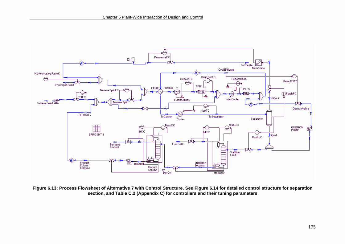
Chapter 6 Plant-Wide Interaction of Design and Control
175
Figure 6.13: Process Flowsheet of Alternative 7 with Control Structure. See Figure 6.14 for detailed control structure for separation section, and Table C.2 (Appendix C) for controllers and their tuning parameters
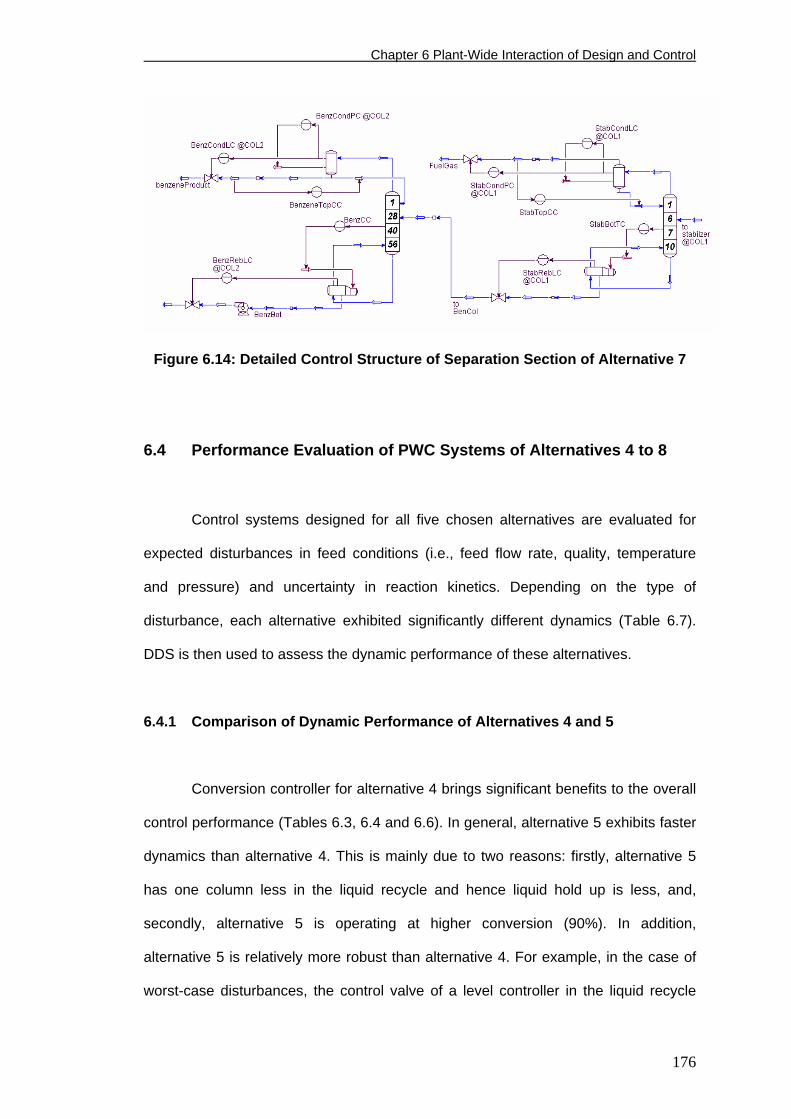
Chapter 6 Plant-Wide Interaction of Design and Control
Figure 6.14: Detailed Control Structure of Separation Section of Alternative 7
6.4 Performance Evaluation of PWC Systems of Alternatives 4 to 8
Control systems designed for all five chosen alternatives are evaluated for
expected disturbances in feed conditions (i.e., feed flow rate, quality, temperature
and pressure) and uncertainty in reaction kinetics. Depending on the type of
disturbance, each alternative exhibited significantly different dynamics (Table 6.7).
DDS is then used to assess the dynamic performance of these alternatives.
6.4.1 Comparison of Dynamic Performance of Alternatives 4 and 5
Conversion controller for alternative 4 brings significant benefits to the overall
control performance (Tables 6.3, 6.4 and 6.6). In general, alternative 5 exhibits faster
dynamics than alternative 4. This is mainly due to two reasons: firstly, alternative 5
has one column less in the liquid recycle and hence liquid hold up is less, and,
secondly, alternative 5 is operating at higher conversion (90%). In addition,
alternative 5 is relatively more robust than alternative 4. For example, in the case of
worst-case disturbances, the control valve of a level controller in the liquid recycle
176
Chapter 6 Plant-Wide Interaction of Design and Control
loop reaches 5% opening for alternative 5 versus 0% opening for alternative 4. Since
it is advisable to operate valves above 10% opening to avoid operational difficulties,
conversion controller is still required for alternative 5, which makes the control
system even more responsive and robust. However, the benefits of conversion
controller for alternative 5 are not as significant as those for alternative 4 (Table 6.6).
This is due to the less recycle effects as the process is operating at relatively high
conversion. Overall, conversion controller is needed for both the alternatives 4 and 5;
alternative 5 is superior to the alternative 4 and observed to be operating closer to
the optimal steady-state. As alternative 4 is less economical and has relatively poorer
control performance than alternative 5 (see Tables 6.1, 6.3, 6.4 and 6.6), for
conciseness, it is excluded from further analysis.
Table 6.6: Comparison of Dynamic Performance of Alternatives 4 and 5
Alternative 4 Alternative 5
With
Conversion Controller
Without Conversion Controller
With Conversion Controller
Without Conversion Controller
DDS for -5% variation
in the Toluene Feed
Flow Rate
8.17 44.92 6.45 10.10
6.4.2 Comparison of Dynamic Performances of Alternatives 5 to 8
Alternatives 5 to 8 are subjected to various anticipated disturbances and the
control performance results are summarized in Table 6.7. In general, the dynamic
performance of each alternative varies with the disturbance. For toluene feed flow
rate variation, the performance of all four alternatives is comparable and alternative 7
exhibits slightly superior performance. A similar conclusion can be made for toluene
177
Chapter 6 Plant-Wide Interaction of Design and Control
feed temperature variation; in this case, however, the performance of alternative 7 is
close to that of the best alternative (alternative 6). In the presence of feed quality
variation, alternatives 7 and 5 are observed to be the best and worst performers
respectively (Figure 6.15). For hydrogen feed pressure variation, alternative 7 is as
good as alternative 6, whereas the poorest performer is alternative 5. In addition,
alternative 7 is the only stable process for the disturbances that are related to
uncertainty in kinetics. Hence, alternative 7 should be chosen from standpoint of
control as it is either superior or competitive with other alternatives for all the
anticipated disturbances. Contrary to the general expectation, alternative 7, which is
slightly more complex due to the presence of two reactors, is found to be dynamically
superior. This may not be recognized without rigorous dynamic simulations. One
reason for the superiority of alternative 7 could be the balanced handling of
disturbances by the two reactors and, hence, the overall impact of disturbance is less
severe.
To conclude, though alternative 8 is found to be the most economical (Table
6.1), dynamic analysis reveals that the alternative 7 exhibits either better or
comparable dynamic performance for all of the anticipated disturbances (Table 6.7).
In addition, alternative 7 is the only alternative that is stable with regard to
uncertainties in the reaction kinetics. As these uncertainties are prevalent, alternative
7 should be the final choice, though it is slightly uneconomical.
178
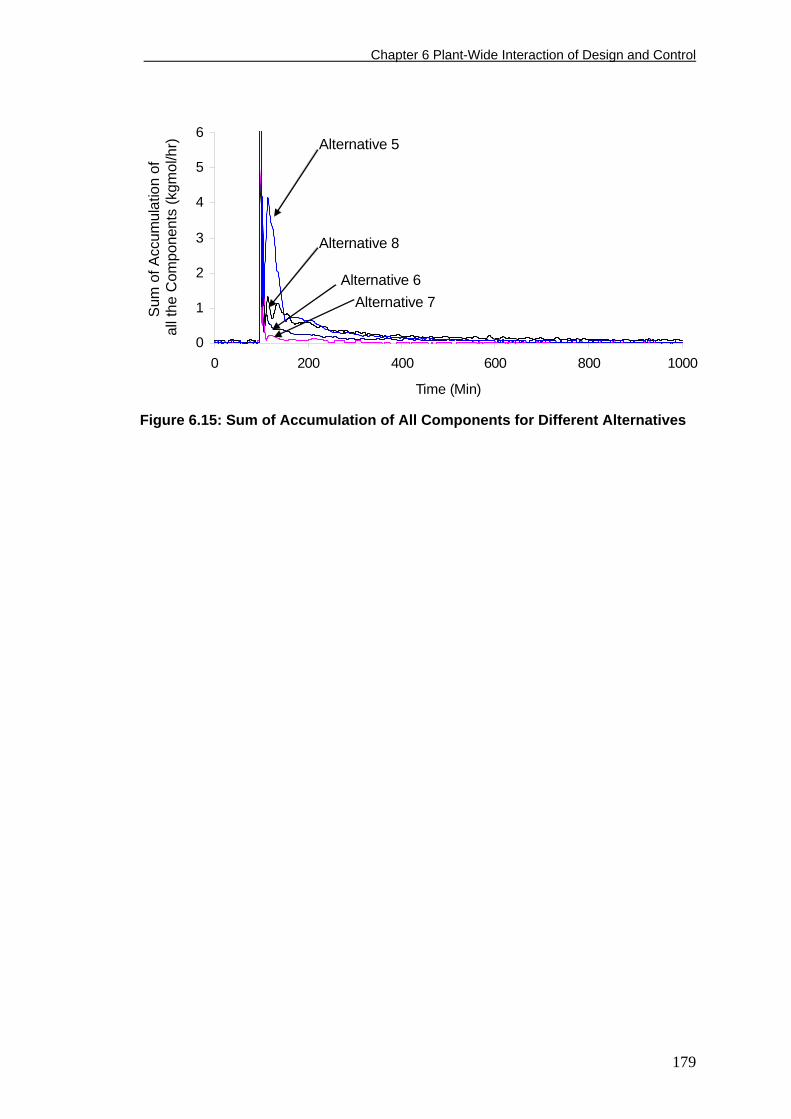
Chapter 6 Plant-Wide Interaction of Design and Control
179
Figure 6.15: Sum of Accumulation of All Components for Different Alternatives
0
1
2
3
4
5
6
0 200 400 600 800 1000
Time (Min)
DD
SS
um o
f Acc
umul
atio
n of
al
l the
Com
pone
nts
(kgm
ol/h
r) Alternative 5
Alternative 8
Alternative 6Alternative 7
0
1
2
3
4
5
6
0 200 400 600 800 1000
Time (Min)
DD
SS
um o
f Acc
umul
atio
n of
al
l the
Com
pone
nts
(kgm
ol/h
r)
Alternative 8
Alternative 5
Alternative 6Alternative 7
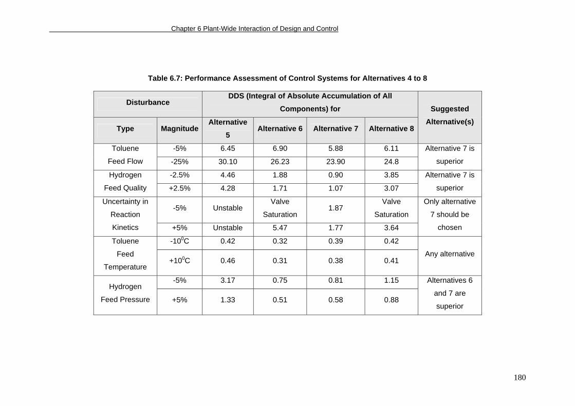
Chapter 6 Plant-Wide Interaction of Design and Control
180
Table 6.7: Performance Assessment of Control Systems for Alternatives 4 to 8
Disturbance DDS (Integral of Absolute Accumulation of All
Components) for
Type MagnitudeAlternative
5 Alternative 6 Alternative 7 Alternative 8
Suggested Alternative(s)
-5% 6.45 6.90 5.88 6.11 Toluene
Feed Flow -25% 30.10 26.23 23.90 24.8
Alternative 7 is
superior
-2.5% 4.46 1.88 0.90 3.85 Hydrogen
Feed Quality +2.5% 4.28 1.71 1.07 3.07
Alternative 7 is
superior
-5% Unstable Valve
Saturation 1.87
Valve
Saturation
Uncertainty in
Reaction
Kinetics +5% Unstable 5.47 1.77 3.64
Only alternative
7 should be
chosen
-100C 0.42 0.32 0.39 0.42 Toluene
Feed
Temperature +100C 0.46 0.31 0.38 0.41
Any alternative
-5% 3.17 0.75 0.81 1.15 Hydrogen
Feed Pressure +5% 1.33 0.51 0.58 0.88
Alternatives 6
and 7 are
superior
Chapter 6 Plant-Wide Interaction of Design and Control
6.5 Summary
A simulation-based heuristic approach for optimal process design and
effective plant-wide control system design is presented and successfully applied to
an industrial case study. The modified design procedure, while retaining all the
benefits of conventional design procedure, is observed to be effective to surface
more design alternatives. For HDA process, the alternatives with the membrane gas
separation unit are found to be economically more attractive. However, the dynamic
performance of some of them is not as good. In general, dynamic/control
performance improves with increasing conversion due to reduced recycle severity.
For the process alternatives with relatively lower optimal conversions (alternatives 4
and 5), conversion controller is desirable to improve the dynamic performance. The
successful application of the integrated framework of Konda et al. (2005) to several
process alternatives demonstrates its capability and generic nature. This study, in
general, demonstrates the practicability of the simulation-based heuristic approach
for the rigorous treatment of integrated design and control studies for industrial
processes. It also emphasizes the conflicts between steady-state economics and
dynamic operability, and highlights the importance of integration of design and
control from plant-wide perspective. The proposed DDS is observed to be a good
measure to quantify the dynamic performance of different process alternatives and
control structures. Use of DDS for quantifying the severity of recycle dynamics is
under investigation. As discussed in section 6.3.4, due to the unavailability of
information on membrane dynamics for gas separations, simplified and yet
appropriate dynamics are assumed for the dynamic simulation of process
alternatives with membrane units. More accurate simulations require further research
on the dynamics of gas membrane units.
181
Chapter 7 Conclusions and Recommendations
CHAPTER 7
CONCLUSIONS AND RECOMMENDATIONS
7.1 Conclusions
PWC system design and several related aspects (such as CDOF,
performance assessment of PWC systems, and interaction between design and
control) are studied in this thesis. The major contributions and conclusions are as
follows.
1. Various PWC methods have been systematically classified based on the
‘approach’ used and the ‘control structure’ considered in each method. This,
in turn, would be useful for researchers to quickly understand the two basic
features of existing methods and develop newer methods (or tailor the
existing methods) to better suit today’s more demanding requirements.
2. A multi-stage integrated framework to design viable PWC systems for
industrial processes has been proposed. One of the important features of this
framework is to systematically analyze and minimize the impact of recycle,
the foe (from control perspective) of many industrial processes, on the overall
process dynamics to improve PWC system performance. This framework is
then successfully applied to one of the industrially-important petrochemical
processes, namely the HDA process. This study demonstrates that the
capabilities of process simulators, paired with heuristics can prove to be a
boon to PWC of industrial processes.
3. A simple and yet effective procedure for CDOF is proposed and applied to
several industrially important processes.
182
Chapter 7 Conclusions and Recommendations
4. A dynamic performance measure, namely DDS, which can be used to assess
the performance of alternative control structures and process designs, is
proposed. It is then used to show the superiority of the proposed PWC
method by comparing the performance of the resulting control system with
that of existing control systems in the literature.
5. A modified sequential approach is proposed to study the impact of process
design on PWC system by integrating the proposed PWC method and
heuristics-based process design procedure. It is shown that the conventional
hierarchical process design procedure needs to be modified to better handle
the increasing complexity of chemical processes and the corresponding
modifications are suggested. The main conclusion here is, though
retrospectively obvious but worth repeating as the plant-wide studies in this
direction are limited, that the most economically attractive process need not
necessarily be the best from operation viewpoint.
7.2 Recommendations for Future Work
PWC is an open-ended problem and there exists scope for many studies.
These are outlined below along with some pointers to pursue them.
Application of Proposed Methodology to Other Industrial Processes and
Further Enhancements: The proposed methodology has been successfully applied
to the HDA process. However, there is a need to apply the proposed method to other
processes to enhance it further. Preliminary studies have been carried on styrene
and vinyl chloride monomer (VCM) processes, which have shown satisfactory
applicability of the proposed integrated framework. Further investigation needs to be
carried out to concretize these observations. The most common test-beds for PWC
183
Chapter 7 Conclusions and Recommendations
are reactor-separator-recycle (RSR) network and the TE process. For example, more
than 60 studies have used the TE process for several applications including PWC,
monitoring, fault detection and online optimization (e.g., Ricker, 1995; Duvall and
Riggs, 2000; Larsson et al., 2001; Jockenhovel et al., 2003; Tian and Hoo, 2003). On
the other hand, till date, there are only a few studies on styrene (e.g., Turkay et al.,
1993) and VCM processes (e.g., Seider et al., 2004). It is therefore worth applying
the proposed integrated framework to these processes.
In the present study, the main emphasis is given to synthesizing plant-wide
decentralized control system with little attention to optimization. So, it is
recommended to study the integration of PWC and optimization to further improve
profitability by optimally operating the process in the presence of disturbances. This
is closely related to plant-wide dynamic optimization or optimal control. A three-tier
integration method is proposed by Lu (2003) recently, which can be a good starting
point in this direction. Alternatively, it is also possible to integrate self-optimizing
control concepts (e.g., Kassidas et al., 2000; Skogestad, 2004) with the proposed
framework.
Study of Reactor-Separator-Recycle (RSR) Network: RSR is one of the
widely used test-beds to carry out PWC studies as it is simple and yet preserves the
general plant-wide nature due to the presence of reactor and separator (either a flash
or distillation column) which are interconnected with a recycle. Despite its simplicity,
there has not been consensus among researchers on its control strategy - for
example, Wu and Yu (1996) suggested a balanced control structure for RSR process
by varying reactor holdup (to keep the reactor composition constant) to avoid
snowball effect. Loperena et al. (2004), however, identified that the balanced control
structure proposed by Wu and Yu (1996) does not eliminate the snowball effect, but
transfers it to other process variables. They have then proposed another balanced
184
Chapter 7 Conclusions and Recommendations
control structure using the reactor temperature as the manipulator to distribute the
impact of disturbance between reactor and separator thereby reducing the snowball
effect. Besides, several control structures have been proposed for RSR network.
Though all these control structures are valid, one may perform better than the other
depending on circumstances. However, clear-cut guidelines are not available on
what strategy to be chosen under what conditions. Besides, most of the work on RSR
in the past has been based on hypothetical processes with simplified kinetics. In a
series of papers, Ward et al. (2004; 2005 & 2006) have recently addressed the
impact of kinetics on control policy, which can be a good basis for the work in this
direction. In addition, other structural decisions, such as the presence of purge
stream, can affect the overall process dynamics (Baldea et al., 2006); the type of
reactor holdup (liquid- or gas-phase) also affects the control decisions (e.g., Larsson,
2000). Thus, a more comprehensive study, considering several issues (e.g.,
presence/absence of purge, type of recycle [gas or liquid], type of reactor holdup
[gas, liquid or both], type of reactions [reversible/irreversible/auto-catalytic]), and their
effects on overall process dynamics and control decisions, needs to be carried out,
using nonlinear dynamic simulations. Steady-state and dynamic models for ethylene-
and propylene-glycol processes have already been developed as part of this work
(Appendix D), and can be used to carry out further study.
Plant-Wide application of advanced control techniques like MPC: The
main emphasis in this thesis is to synthesize a basic regulatory control system based
on PID controllers but advanced control techniques (such as MPC or its variants like
DMC) are not considered. This is justifiable as the regulatory control system is the
basic criterion even for the advanced control techniques. Having successfully
developed the basic regulatory control system for the HDA process, the next step
would be developing advanced control strategies for the entire plant. In general,
plant-wide application of advanced control techniques are relatively limited (Doyle et
185
Chapter 7 Conclusions and Recommendations
al., 1997). An attempt in this direction is by Ricker and Lee (1995) who applied
nonlinear model predictive control to the TE process. Later, Ricker (1996) observed
that the NMPC has only a marginal improvement over the decentralized control
system. He has also observed that the decentralized control system does a better job
of handling constraints – an area in which NMPC is reputed to excel. So, it is of
interest to see whether the advanced control techniques can improve the
performance over the regulatory control system in the case of the highly integrated
HDA process. Lately, Gonzalez et al. (2006) applied MPC to heat-exchanger
networks. One main commonality between any PWC problem and heat-exchanger
network control problem is that both of them are highly integrated with the presence
of recycles. Thus, the work by Gonzalez et al. (2006) can be a good starting point in
this direction.
In general, plant-wide implementation of a single MPC may not always be
feasible due to computational limitations, implementation and other practical
difficulties (Vadigepalli and Doyle, 2003; Baldea et al., 2006). These difficulties
include, but not limited to, insufficient information and difficulty in obtaining the
models of certain process phenomena. So, it is often recommended to implement
multiple MPCs instead, which is known as decentralized or cooperative plant-wide
MPC. In this approach, co-ordination among different MPCs is important to achieve
satisfactory overall performance. Recently, Cheng et al. (2005) have proposed a
price-driven approach to efficiently co-ordinate decentralized MPCs, and Motee and
Rodsari (2003) presented an algorithm for optimal partitioning; these can form a
basis for further work in this direction. Another challenging aspect of this study is the
identification of plant-wide models to implement MPC.
Economic Quantification of Dynamic Performance: Though interaction
between design and control is studied in this work (Chapter 6), economic
186
Chapter 7 Conclusions and Recommendations
quantification of the dynamic performance is not explicitly used as there is only one
process design alternative which is dynamically stable (for all the anticipated
disturbances) for this case study (i.e., the HDA process). However, there may be
more than one process alternative which are dynamically stable for other case
studies. Hence, to make this study more comprehensive and generic, it is very much
needed to economically quantify dynamic performance, which eventually helps to
better understand the interaction between design and control. Zheng and Mahajanam
(1999) proposed a method to quantify the cost associated with dynamic controllability
based on minimum additional surge capacity that is required to meet all of the control
objectives and constraints dynamically for all of the expected disturbances, which is a
good starting point to work in this direction. The basic idea is to economically quantify
the dynamic performance using DDS so that it can appropriately be integrated with
the proposed approach to study interaction between design and control.
187
REFERENCES
Alhammadi, H. Y.; Romagnoli, J. A. Process Design and Operation: Incorporating
Environmental, Profitability, Heat Integration and Controllability Considerations. In
The Integration of Process Design and Control, ed by Seferlis, P. and Georgiadis,
M. C., pp. 264-305. Elsevier: Amsterdam. 2004.
Baker, R. W. Future Directions of Membrane Gas Separation Technology, Ind. Eng.
Chem. Res., 41, pp. 1393-1411. 2002.
Balasubramanian, P.; Kosuri, M. R.; Pushapavanam, S.; Kienle, A. Effect of Delay on
the Stability of a Coupled Reactor-Separator System, Ind. Eng. Chem. Res., 42,
pp. 3758-3764. 2003.
Baldea, M.; Daoutidis, P.; Kumar, A. Dynamics and Control of Integrated Networks
with Purge Streams, AIChE J., 52, pp. 1460-1472. 2006.
Banerjee, A.; Arkun, Y. Control Configuration Design Applied to the Tennessee
Eastman Plant-Wide Control Problem, Comput. Chem. Eng., 19, pp. 453-480.
1995.
Barrero, L.; Canales, R.; Romero, D. J.; Mendoza, Y.; Ruiz, G.; Gutierrez, S. S ;
Systematic Building-Testing of Dynamic Models for Training Simulators, Comput.
Chem. Eng., 27, pp. 1421-1430. 2003.
Benyahia, F. Flowsheeting Packages: Reliable or Fictitious Process Models?, Trans.
IChemE., 78 (Part A), pp. 840-844. 2000.
Bequette, W. B. Process Control: Modeling, Design and Simulation. New Jersey:
Prentice Hall. 2003.
Bildea, C. S.; Dimian, A. C.; Iedema, P. D. Nonlinear Behavior of Reactor-Separator-
Recycle Systems, Comput. Chem. Eng., 24, pp. 209-215. 2000.
Bishop, T.; Chapeaux, M.; Jaffer, L.; Nair, K.; Patel, S. Ease Control Valve Selection,
Chem. Eng. Prog., November, pp. 52-56. 2002.
188
Blevins, T. L.; McMillan, G. K.; Wojsznis, W. K.; Brown, M. W. Advanced Control
Unleashed: Plant Performance Management for Optimum Benefit. pp. 41-42, NC:
ISA. 2003.
Buckley, P. S. Techniques of Process Control. New York: Wiley. 1964.
Cao, Y., Biss, D.; Perkins, J.D. Assessment of Input-Output Controllability in the
Presence of Control Constraints, Comput. Chem. Eng., 20, pp. 337-346. 1996.
Cao, Y.; Rossister, D.; Owens, D. Input Selection for Disturbance Rejection under
Manipulated Variable Constraints, Comput. Chem. Eng., 21, pp. S403-S408.
1997.
Cao, Y.; Rossister, D. An Input Pre-Screening Technique for Control Structure
Selection, Comput. Chem. Eng., 21, pp. 563-569. 1997.
Cao, Y.; Rossister, D. Input Selection and Localized Disturbance Rejection, J.
Process Control, 8, pp. 175-183. 1998.
Carlson, E. C. Don’t Gamble with Physical Properties for Simulations. Chem. Eng.
Prog. 1996, 37-46.
Castro, J. J.; Doyle III, F. J. Plantwide Control of the Fiber Line in a Pulp Mill, Ind.
Eng. Chem. Res., 41, pp. 1310-1320. 2002.
Castro, J. J.; Doyle III, F. J. A Pulp Mill Benchmark Problem for Control: Application
of Plantwide Control Design, J. Process Control, 14, pp. 329-347. 2004.
Chen, R.; McAvoy, T. Plantwide Control System Design: Methodology and
Application to a Vinyl Acetate Process, Ind. Eng. Chem. Res., 42, pp. 4753-4771.
2003.
Chen, Y. H.; Yu, C. C. Design and Control of Heat-Integrated Reactors, Ind. Eng.
Chem. Res., 42, pp. 2791-2808. 2003.
Chen, R.; McAvoy, T.; Zafiriou, E. Plantwide Control System Design: Extension to
Multiple-Forcing and Multiple-Steady-State Operation, Ind. Eng. Chem. Res., 43,
3685-3694. 2004.
189
Chen, J.; Adomaitis, R. A. An Object-Oriented Framework for Modular Chemical
Process Simulation with Semiconductor Processing Applications, Comput. Chem.
Eng., 30, pp. 1354-1380. 2006.
Cheng, R.; Forbes, F.; Yip, W. S. Price-Driven Coordination for solving Plant-Wide
MPC Problems. In Proc. 16th International Federation of Automatic Control, July
2005, Prague, Czech Republic.
Cheng, Y. C.; Yu, C. C. Effects of Process Design on Recycle Dynamics and its
Implication to Control Structure Selection, Ind. Eng. Chem. Res., 42, pp. 4348-
4365. 2003.
Chien, I. L.; Zeng, K. L.; Chao, H. Y. Design and Control of a Complete
Heterogeneous Azeotropic Distillation Column System, Ind. Eng. Chem. Res., 43,
pp. 2160-2174. 2004.
Chodavarapu, S. K.; Zheng, A., Control System Design for Recycle Systems, J.
Process Control, 11, pp. 459-468. 2001.
Chodavarapu, S. K.; Zheng, A. A Definition of Steady-State Plant-Wide
Controllability. Ind. Eng. Chem. Res., 41, pp. 4338-4345. 2002.
Cole, J. D. and Yount, K. B. Applications of Dynamic Simulation to Industrial Control
Problems, ISA Trans., 33, pp. 11-18. 1994.
Conradie, A. V. E.; Aldrich, C. Neurocontrol of a Ball Mill Grinding Circuit Using
Evolutionary Reinforcing Learning, Miner. Eng., 14, pp. 1277-1294. 2001.
Cuellar, B. D. M.; Villa, M. V.; Puebla, H.; Ramirez, J. A. Model Approximation for
Dead-Time Recycling Systems, Ind. Eng. Chem. Res., 44, pp. 4336-4343. 2005.
Davidson, J.; Bertele, O. V. Process pump selection: a systems approach. Bury St.
Edmunds: Professional Engineering Publishing Limited. 2000.
Denn, M. M.; Lavie, R. Dynamics of Plants with Recycle, Chem. Eng. J., 24, pp. 55-
59. 1982.
190
Dimian, A. C.; Groenendijk, A. J.; Iedema, P.D. Recycle Interaction Effects on the
Control of Impurities in a Complex Plant, Ind. Eng. Chem. Res., 40, pp. 5784-
5794. 2001.
Dimian, A. C. Integrated Design and Simulation of Chemical Processes. Boston:
Elsevier. 2003.
Diwekar, U. M.; Madhavan, K. P. BATCH-DIST: A Comprehensive Package for
Simulation, Design, Optimization and Optimal Control of Multicomponent,
Multifraction Batch Distillation Columns, Comput. Chem. Eng., 15, pp. 833-842.
1991.
Douglas, J. M. Process Operability and Control of Preliminary Designs. In Chemical
Process Control – II, Proceedings of Engineering Foundation Conference, ed by
Seborg, D. E. and Edgar, T. F., 1981, Sea Island, Ga. pp. 497-524.
Douglas, J. M. A Hierarchical Decision Procedure for Process Synthesis, AIChE J.
31, pp. 353-362. 1985.
Douglas, J. M. Conceptual Design of Chemical Processes. New York: McGraw-Hill.
1988.
Doyle III, F. J.; Pekny, J. F.; Dave, P.; Bose, S. Specialized Programming Methods in
the Model Predictive Control of Large Scale Systems, Comput. Chem. Eng., 21,
pp. S847-S852. 1997.
Downs, J. J. Distillation Control in a Plantwide Control Environment. In Practical
Distillation Control, ed by Luyben, W. L., pp. 413-439. New York: Van Nostrand
Reinhold. 1992.
Downs, J.; Vogel, E., A Plantwide Industrial Process Control Problem, Comput.
Chem. Eng., 17, pp. 245-255. 1993.
Duvall, P. M.; Riggs, J. B. On-line Optimization of the Tennessee Eastman Challenge
Problem, J. Process Control, 10, pp. 19-33. 2000.
191
Elliott, T. R.; Luyben, W. L. Capacity-Based Economic Approach for the Quantitative
Assessment of Process Controllability during the Conceptual Design Stage, Ind.
Eng. Chem. Res., 34, pp. 3907-3915. 1995.
Elliott. T. R.; Luyben, W. L. Quantitative Assessment of Controllability during the
Design of a Ternary System with Two Recycle Streams, Ind. Eng. Chem. Res.,
35, pp. 3470-3479. 1996.
Elliott, T. R.; Luyben, W. L. Application of the Capacity-Based Economic Approach to
an Industrial-Scale Process, Ind. Eng. Chem. Res., 36, pp. 1727-1737. 1997.
Emets, S. V. An Examination of a Modified Hierarchical Design Structure for
Chemical Processes. MS Thesis, Chemical Engineering Department, Texas Tech
University, 2003. (Available at
http://www.che.ttu.edu/classes/che5000/EmetsThesis.pdf, accessed in January
2004.)
Emets, S. V.; Hoo, K. A.; Mann, U. A Modified Hierarchy for Designing Chemical
Processes, Ind. Eng. Chem. Res., 45, pp. 5037-5043. 2006.
Fabro, J. A.; Arruda, L. V. R.; Neves Jr. F.; Startup of a Distillation Column Using
Intelligent Control Techniques, Comput. Chem. Eng., 30, pp. 309-320. 2005.
Feliu, J. A.; Grau, I.; Alos, M. A.; Hernandez, J. J. M. Match Your Process
Constraints Using Dynamic Simulation, Chem. Eng. Prog., December, pp. 42-48.
2003.
Fisher, W. R.; Doherty, M. F.; Douglas, J. M. The Interface between Design and
Control. 3. Selecting a Set of Controlled Variables, Ind. Eng. Chem. Res., 27, pp.
611-615. 1988.
Fonyo, Z. Design Modifications and Proper Plantwide Control, Comput. Chem. Eng.,
18, pp. S483-S492. 1994.
Foss, A.S. Critique of Chemical Process Control Theory, AIChE J.,19 (2), pp. 209-
214. 1973.
192
Garelli, F.; Mantz, R. J.; Battista, H. D. Limiting Interactions in Decentralized Control
of MIMO Systems, J. Process Control, 16, pp. 473-483. 2006.
Georgakis, C.; Uzturk, D.; Subramanian, S.; Vinson, D. R. On the Operability of
Continuous Processes, Control Eng. Pract., 11, pp. 859-869. 2003.
Gilliland, E. R.; Reed, C. E. Degrees of Freedom in Multicomponent Absorption and
Rectification Columns, Ind. Eng. Chem., 34, pp. 551-557. 1942.
Gilliland, E. R.; Goud, L. A.; Boyle, T. J. Dynamic Effects of Material Recycle. In
Preprints of Joint Automatic Control Conference, 1964, California, USA, pp. 140-
146.
Goel, H. D.; Grievink, J.; Herder, P. M.; Weijnen, M. P. C. Integrating Reliability
Optimization into Chemical Process Synthesis, Reliab. Eng. Syst Saf., 78, pp.
247-258. 2002.
Gonzalez, A. H.; Odloak, D.; Marchetti, J. L. Predictive Control Applied to Heat-
Exchanger Networks, Chem. Eng. Process., 45, pp. 661–671. 2006.
Govind, R.; Powers, G. J. Control System Synthesis Strategies, AIChE J., 28, pp. 60-
73. 1982.
Grassi, V. G. Dynamic Simulation as a Tool to Integrate Process Design and Process
Control, ISA Trans., 32, pp. 323-332. 1993.
Groenendijk, A. J.; Dimian, A. C.; Iedema, P. D. Systems Approach for Evaluating
Dynamics and Plant-Wide Control of Complex Plants, AIChE J., 46, pp. 133-145.
2000.
He, M. J.; Cai, W. J. New Criterion for Control-Loop Configuration of Multivariable
Processes, Ind. Eng. Chem. Res., 43, pp. 7057-7064. 2004.
Heath, J. A.; Kookos, I. K.; Perkins, J. D. Process Control Structure Selection based
on Economics, AIChE J., 46, pp. 1998-2016. 2000.
Henry, R. M.; Mujtaba, I. M. Distillation Column Control: The Use of Feed
Temperature to Respond to Modest Variations in Feed Composition, Comput.
Chem. Eng., 23, pp. S265-S268. 1999.
193
Herrmann, G.; Spurgeon, S. K.; Edwards, C. A Model-Based Sliding Mode Control
Methodology Applied to the HDA-Plant, J. Process Control, 13, pp. 129-138.
2003.
Horwitz, B. A.; Nocera, A. J. Are You “Scotomatized” by Your Simulation Software?,
Chem. Eng. Prog., September, pp. 68-71. 1996.
Hugo, A. J.; Taylor, P. A.; Wright, J. D. Approximate Dynamic Models for Recycle
Systems, Ind. Eng. Chem. Res., 35, pp. 485-487. 1996.
Jacobsen, E. W. Effect of Recycle on the Plant Zero Dynamics. Comput. Chem.
Eng., 21, pp. S279-S284, 1997.
Jang, W. H.; Hahn, J.; Hall, K. R. Genetic/Quadratic Search Algorithm for Plant
Economic Optimizations Using a Process Simulator, Comput. Chem. Eng., 30,
pp. 285-294. 2005.
Jockenhovel, T.; Biegler, L. T.; Wachter, A. Dynamic Optimization of the Tennessee
Eastman Process Using The OptControlCentre, Comput. Chem. Eng., 27, pp.
1513-1531. 2003.
Johns, W. R. Process Synthesis: Poised for a wider role, Chem. Eng. Prog., April, pp.
59-65. 2001.
Jorgensen, J. B.; Jorgensen, S. B. Towards Automatic Decentralized Control
Structure Selection, Comput. Chem. Eng., 24, pp. 841-846. 2000.
Kanadibhotla, R. S.; Riggs, J. B. Nonlinear Model Based Control of a Recycle
Reactor Process, Comput. Chem. Eng., 19, pp. 933-948. 1995.
Kao, Y. K.; Yan, Z. Dynamic Modeling and Simulation of Simple Membrane
Permeators, Chem. Eng. Commun., 59, pp. 343-370. 1987.
Kapoor, N.; McAvoy, T. J.; Marlin, T. E. Effect of Recycle Structure on Distillation
Tower Time Constants, AIChE J., 32, pp. 411-418. 1986.
Kassidas, A.; Patry, J.; Marlin, T. Integrating Process and Controller Models for the
Design of Self-Optimizing Control, Comput. Chem. Eng., 24, pp. 2589-2602.
2000.
194
Keller, G. E.; Bryan, P. F. Process Engineering Moving in New Directions, Chem.
Eng. Prog., January, pp. 41-50. 2000.
Kim, Y.; Lee, B.; Eo, S.; Yoon, E. S. A Study on the Evaluation and Improvement of
Structural Controllability of Chemical Processes, Comput. Chem. Eng., 24, pp.
931-936. 2000.
Kocis, G. R.; Grossmann, I. E. A Modeling and Decomposition Strategy for the
MINLP Optimization of Process Flowsheets., Comput. Chem. Eng., 13, pp. 797-
819. 1989.
Konda, N. V. S. N. M.; Rangaiah, G. P.; Krishnaswamy, P. R. Systematic
Classification of Plant-Wide Control System Design Procedures with Application
to the HDA Process, Presented at AIChE Annual Meeting, Nov. 2003, San
Francisco, USA.
Konda, N. V. S. N. M.; Rangaiah, G. P.; Krishnaswamy, P. R. Plant-Wide Control of
Industrial Processes: An Integrated Framework of Simulation and Heuristics, Ind.
Eng. Chem. Res., 44, pp. 8300-8313. 2005.
Konda, N. V. S. N. M.; Rangaiah, G. P.; Krishnaswamy, P. R. A Simple and Effective
Procedure for Control Degrees of Freedom, Chem. Eng. Sci., 61, pp. 1184-1194.
2006.
Konda, N. V. S. N. M.; Rangaiah, G. P.; Lim, D. K. H. Optimal Process Design and
Effective Plant-Wide Control of Industrial Processes by Simulation-based
Heuristic Approach, Ind. Eng. Chem. Res., 45, pp. 5955-5970. 2006.
Konda, N. V. S. N. M.; Rangaiah, G. P. Performance Assessment of Plant-Wide
Control Systems of Industrial Processes, Ind. Eng. Chem. Res., 46, pp. 1220-
1231. 2007.
Kookos, I. K.; Perkins, J. D. Heuristic-Based Mathematical Programming Framework
for Control Structure Selection, Ind. Eng. Chem. Res., 40, pp. 2079-2088. 2001a.
Kookos, I. K.; Perkins, J. D. An Algorithm for Simultaneous Process Design and
Control, Ind. Eng. Chem. Res., 40, pp. 4079-4088. 2001b.
195
Kookos, I. K.; Perkins, J. D. An Algorithmic Method for the Selection of Multivariable
Process Control Structures, J. Process Control, 12, pp. 85-99. 2002.
Kumar, A.; Daoutidis, P. Nonlinear Dynamics and Control of Process Systems with
Recycle, J. Process Control, 12, pp. 475-484. 2002.
Kwauk, M. A System for Counting Variables in Separation Processes, AIChE J., 2,
pp. 240-248. 1956.
Laganier, F. Dynamic Process Simulation Trends and Perspectives in an Industrial
Context, Comput. Chem. Eng., 20, pp. S1595-S1600, 1996.
Lakshminarayanan, S.; Takada, H. Empirical Modelling and Control of Processes
with Recycle: Some Insights via Case Studies, Chem. Eng. Sci., 56, pp. 3327-
3340. 2001.
Lakshminarayanan, S.; Onodera, K.; Madhukar, G. M. Recycle Effect Index: A
Measure to Aid in Control System Design for Recycle Processes, Ind. Eng.
Chem. Res., 43, pp. 1499-1511. 2004.
Larsson, T. Studies on Plantwide Control. Dr.Ing. Thesis, Department of Chemical
Engineering, Norwegian University of Science and Technology. 2000.
Larsson, T.; Hesteturn, K.; Hovland, E.; Skogestad, S. Self-Optimizing Control of a
Large-Scale Plant: The Tennessee Eastman Process, Ind. Eng. Chem. Res., 40,
pp. 4889-4901. 2001.
Larsson, T.; Govtsmark, M. S.; Skogestad, S.; Yu, C. C. Control Structure Selection
for Reactor, Separator, and Recycle Processes, Ind. Eng. Chem. Res., 42, pp.
1225-1234. 2003.
Lausch, H. R.; Wozny, G.; Wutkewicz, M.; Wendeler. H. Plant-Wide Control of an
Industrial Process, Trans. IChemE., 76, Part A. pp. 185-192. 1998.
Lee, P. L.; Li, H.; Cameron, I. T. Decentralized Control Design for Nonlinear Multi-
Unit Plants: A Gap Metric Approach, Chem. Eng. Sci., 55, pp. 3743-3758. 2000.
196
Liggin, W. L. UOP Thermal Hydrodealkylation (THDA) Process. In Handbook of
Petroleum Refining Processes, ed by Meyers, R. A., pp. 2.23-2.26. New York:
McGraw-Hill. 1997.
Longwell, E. J. Dynamic Modeling for Process Control and Operability, ISA Trans.,
33, pp. 3-10. 1994.
Loperena, R. M.; Solar, R.; Ramirez, J. A. Balanced Control Scheme for
Reactor/Separator Processes with Material Recycle, Ind. Eng. Chem. Res., 43,
pp. 1853-1862. 2004.
Lu, J. Z. Challenging Control Problems and Emerging Technologies in Enterprise
Optimization, Control Eng. Pract., 11, pp. 847-858. 2003.
Luyben, W. L. Process Modeling, Simulation, and Control for Chemical Engineers.
pp. 15-162, New York: McGraw-Hill. 1990.
Luyben, W.L. Dynamics and Control of Recycle Systems. 1. Simple Open-loop and
Closed-Loop Systems, Ind. Eng. Chem. Res., 32, pp. 466-475. 1993.
Luyben, M. L.; Floudas, C. A. Analyzing the Integration of Design and Control – 2.
Reactor-Separator-Recycle System, Comput. Chem. Eng., 18, pp. 971-994.
1994.
Luyben, W. L. Design and Control Degrees of Freedom, Ind. Eng. Chem. Res., 35,
pp. 2204-2214. 1996.
Luyben, M. L.; Tyreus, B. D.; Luyben, W. L. Plantwide Control Design Procedure,
AIChE J., 43, pp. 3161-3174. 1997.
Luyben, W. L. External Versus Internal Open-Loop Unstable Processes, Ind. Eng.
Chem. Res., 37, pp. 2713–2720. 1998.
Luyben, W. L.; Tyreus, B. D.; Luyben, M. L. Plantwide Process Control. New York:
McGraw-Hill. 1999.
Luyben, W. L. Inherent Dynamic Problems with On-Demand Control Structures, Ind.
Eng. Chem. Res., 38, pp. 2315-2329. 1999.
197
Luyben, W. L. Control of Outlet Temperature in Adiabatic Tubular Reactors, Ind. Eng.
Chem. Res., 39, pp. 1271-1278. 2000a.
Luyben, W. L. Design and Control of Gas-Phase Reactor/Recycle Processes with
Reversible Exothermic Reactions, Ind. Eng. Chem. Res., 39, pp. 1529-1538.
2000b.
Luyben, W. L. Impact of Reaction Activation Energy on Plant-Wide Control Structures
in Adiabatic Tubular Reactor Systems, Ind. Eng. Chem. Res., 39, pp. 2345-2354.
2000c.
Luyben, W. L. Effect of Design and Kinetic Parameters on the Control of Cooled
Tubular Reactor Systems, Ind. Eng. Chem. Res., 40, pp. 3623-3633. 2001.
Luyben, W. L. Plantwide Dynamic Simulators in Chemical Processing and Control,
New York: Marcel Dekker. 2002.
Luyben, W. L.; Hendershot, D. C. Dynamic Disadvantages of Intensification of
Inherently Safer Process Design, Ind. Eng. Chem. Res., 43, pp. 384-396. 2004.
Lyman, P. R.; Georgakis, C. Plantwide Control of the Tennessee Eastman Problem,
Comput. Chem. Eng., 19, pp. 321-331. 1995.
Lyman, P. R.; Luyben, W. L. Method for Assessing the Effect of Design Parameters
on Controllability, Ind. Eng. Chem. Res., 35, pp. 3484-3497. 1996.
Mahajanam, R. V.; Zheng, A. Evaluation of Cost of Dynamic Controllability and
Optimal Surge Capacity without Dynamic Models, Ind. Eng. Chem. Res., 41, pp.
3877-3883. 2002.
Mandler, J. A. Modeling for Control Analysis and Design in Complex Industrial
Separation and Liquefaction Processes, J. Process Control, 10, pp. 167-175.
2000.
Marlin, T. E. Process Control: Designing Processes and Control Systems for
Dynamic Performance, Singapore: McGraw-Hill, 1995.
Martinson, W. S.; Barton, P. I. Distributed Models in Plantwide Dynamic Simulators.
AIChE J., 47, pp. 1372-1386. 2001.
198
Marquardt, W. Dynamic Process Simulation - Recent Progress and Future
Challenges, In Proc. of the Fourth International Conference on Chemical Process
Control, Feb. 1991, Texas, USA, pp. 131-180.
McAvoy, T. J.; Ye, N. Base Control for the Tennessee Eastman Problem, Comput.
Chem. Eng., 18, pp. 383-413. 1994.
McAvoy, T. J.; Ye, N.; Gang, C. Nonlinear Inferential Parallel Cascade Control, Ind.
Eng. Chem. Res., 35, pp. 130-137. 1996.
McAvoy, T. J. Synthesis of Plantwide Control Systems Using Optimization, Ind. Eng.
Chem. Res., 38, pp. 2984-2994. 1999.
McGuire, J. T. Pumps for Chemical Processing, New York: Marcel Dekker. 1990.
McKetta, J.J. (ed). Encyclopedia of Chemical Processing and Design. pp. 183-235,
New York: Marcel Dekker. 1977.
Meadowcroft, T. A.; Stephanopoulos, G.; Brosilow, C. The Modular Multivariable
Controller: 1: Steady-State Properties., AIChE J., 38, pp. 1254-1277. 1992.
Meeuse, F. M.; Grievink, J. Thermodynamic Controllability Assessment in Process
Synthesis. In The Integration of Process Design and Control, ed by Seferlis, P.
and Georgiadis, M. C., pp. 146-167. Amsterdam: Elsevier. 2004.
Meindersma, G. W. Membrane Permeation and Pressure Swing Adsorption (PSA) for
the Production of High Purity Hydrogen. In Effective Industrial Membrane
Processes: Benefits and Opportunities, ed by Turner, M. K., pp. 391-400. New
York: Elsevier Applied Science. 1991.
Mizsey, P.; Kalmar, I. Effects of Recycle on Control of Chemical Processes, Comput.
Chem. Eng., 20, pp. S883-S888. 1996.
Moore, C. F. Selection of Controlled and Manipulated Variables. In Practical
Distillation Control, ed by Luyben, W. L., pp. 413-439. New York: Van Nostrand
Reinhold. 1992.
Morari, M.; Arkun, Y.; Stephanopoulos, G. Studies in the Synthesis of Control
Structures for Chemical Processes. Part 1: Formulation of the Problem. Process
199
Decomposition and the Classification of the Control Tasks. Analysis of the
Optimizing Control Structures, AIChE J., 26, pp. 220-232. 1980.
Morud, J.; Skogestad, S. Effects of Recycle on Dynamics and Control of Chemical
Processing Plants, Comput. Chem. Eng., 18, pp. S529-S534. 1994.
Morud, J.; Skogestad, S. Dynamic Behavior of Integrated Plants, J. Process Control,
6, pp. 145-146. 1996.
Motee, N.; Rodsari, B. S. Optimal Partitioning in Distributed Model Predictive Control.
In Proceedings of the American Control Conference, June 2003, Denver, CO.
Mullins, E.; Oldland, R.; Liu, Y. A.; Wang, S.; Sandler, S. I.; Chen, C. C.; Zwolak, M.;
Seavey, K. C. Sigma-Profile Database for Using COSMO-Based Thermodynamic
Methods, Ind. Eng. Chem. Res., 45, pp. 4389-4415. 2006.
Nakagawa, T. Industrial Applications of Membranes for Gas Separation in Japan. In
Polymeric Gas Separation Membranes, ed by Paul, D. R. and Yampolskii, Y. P.,
Boca Raton, FL: CRC Press. 1994.
Narraway, L. T.; Perkins, J. D.; Barton, G. W. Interaction between Process Design
and Process Control: Economic Analysis of Process Dynamics. J. Process
Control, 1, pp. 243-250. 1991.
Narraway, L. T.; Perkins, J.D. Selection of Process Control Structure Based on
Linear Dynamic Economics, Ind. Eng. Chem. Res., 32, pp. 2681-2692. 1993.
Narraway, N.; Perkins, J.D. Selection of Process Control Structures Based on
Economics, Comput. Chem. Eng., 18, pp. S511-S515. 1994.
Nelson, D. A.; Douglas, J. M. A Systematic Procedure for Retrofitting Chemical
Plants to Operate Utilizing Different Reaction Paths, Ind. Eng. Chem. Res., 29,
pp. 819-829. 1990.
Newell, R. B.; Lee, P. L. Applied Process Control: A Case Study. New York: Prentice
Hall. 1989.
Ng, C. S.; Stephanopoulos, G. Synthesis of Control Systems for Chemical Plants,
Comput. Chem. Eng., 20, pp. S999-S1004. 1996.
200
Oh, M.; Pantelides, C. C. A Modeling and Simulation Language for Combined
Lumped and Distributed Parameter Systems, Comput. Chem. Eng. 20, pp. 611-
633. 1996.
Papadourakis, A., Doherty, M. F. and Douglas, J.M. Relative Gain Array for Units in
Plants with Recycle, Ind. Eng. Chem. Res., 26, pp.1259-1262. 1987.
Peng, D. Y.; Robinson, D. B. A New Two-Constant Equation of State, Ind. Eng.
Chem. Fundam., 15, pp. 59-64. 1976.
Perkins, J. D.; Walsh, S. P. K. Optimization as a Tool for Design/Control Integration,
Comput. Chem. Eng., 20, pp. 315-323. 1996.
Pham, Q. T. Degrees of Freedom of Equipment and Processes, Chem. Eng. Sci., 49,
pp. 2507-2512. 1994.
Phimister, J. R.; Fraga, E. S.; Ponton, J. W. The Synthesis of Multistep Process Plant
Configurations, Comput. Chem. Eng., 23, pp. 315-326. 1999.
Ponton, J. W.; Laing, D. M. A Hierarchical Approach to the Design of Process Control
Systems, Trans. IChemE., 17, pp. 181-188. 1993.
Ponton, J. W. Degrees of Freedom Analysis in Process Control, Chem. Eng. Sci., 49,
pp. 2089-2095. 1994.
Prasad, R.; Shaner, R. L.; Doshi, K. J. Comparison of Membranes with other Gas
Separation Technologies. In Polymeric Gas Separation Membranes, ed by Paul,
D. R. and Yampolskii, Y. P., pp. 513-614. Boca Raton, FL: CRC Press. 1994.
Price, R. M. and Georgakis. C. Plantwide Regulatory Control Design Procedure
Using Tiered Framework, Ind. Eng. Chem. Res., 32, pp. 2693-2705. 1993.
Price, R. M.; Lyman, P. R.; Georgakis. C. Throughput Manipulation in Plantwide
Control Structures, Ind. Eng. Chem. Res., 33, pp.1197-1207. 1994.
Qiu, Q. F.; Rangaiah, G.P.; Krishnaswamy, P.R. Application of a Plant-Wide Control
Design to the HDA Process, Comp. Chem. Eng., 27, pp. 73-94. 2003.
201
Reyes, F.; Luyben, W. L. Steady-State and Dynamic Effects of Design Alternatives in
Heat-Exchanger/Furnace/Reactor Processes, Ind. Eng. Chem. Res., 39, pp.
3335-3346. 2000.
Reyes, F.; Luyben, W. L. Design and Control of a Gas-Phase Adiabatic Tubular
Reactor Process with Liquid Recycle, Ind. Eng. Chem. Res., 40, pp. 3762-3774.
2001.
Ricker, N. L. Optimal Steady-State Operation of the Tennessee Eastman Challenge
Process, Comput. Chem. Eng., 19, pp. 949-959. 1995.
Ricker, N. L.; Lee, J. H. Nonlinear Model Predictive Control of the Tennessee
Eastman Challenge Process, Comput. Chem. Eng., 19, pp. 961-981. 1995.
Ricker, N. L. Decentralized Control of The Tennessee Eastman Challenge Problem,
J. Process Control, 6, pp. 205-221. 1996.
Riggs, J. B. Chemical Process Control. Texas: Ferret. 2001.
Riley, K. F.; Hobson, M. P.; Bence, S. J. Mathematical Methods for Physics and
Engineering: A Comprehensive Guide. p. 432, Cambridge: Cambridge University
Press. 2002.
Robinson. D.; Chen. R.; McAvoy, T.; Schnelle. P. D. An Optimal Control Based
Approach to Designing Plantwide Control System Architectures, J. Process
Control, 11, pp. 223-236. 2001.
Rodriguez, M.; Marcos, A. Plantwide Control Design Using an Expert System. In
Proceedings of IFAC 15th Triennial World Congress, 2002. Barcelona, Spain.
Rodriguez, M. A New Algorithm to Develop Hybrid Systems, Comput. Chem. Eng.,
30, pp. 260-267. 2005.
Rudd, D. F.; Watson, C. C. Strategy of Process Engineering. New York: Wiley. 1968.
Sakizlis, V.; Perkins, J. D.; Pistikopoulos, E. N. Recent Advances in Optimization-
based Simultaneous Process and Control Design, Comput. Chem. Eng., 28, pp.
2069-2086. 2004.
202
Samyudia, Y.; Lee, P. L.; Cameron, I. T. Green, M. Control of Multi-Unit Processing
Plants – A Systematic Methodology, Comput. Chem. Eng., 20, pp. S919-S924.
1996.
Scali, C.; Antonelli, R. Performance of Different Regulators for Plants with Recycle,
Comput. Chem. Eng., 19, pp. S409-414. 1995.
Scali, C.; Ferrari, F. Control of Systems with Recycle by means of Compensators,
Comput. Chem. Eng., 21, pp. S267-S272. 1997.
Scali, C.; Ferrari, F. Performance of Control Systems based on Recycle
Compensators in Integrated Plants, J. Process Control, 9, pp. 425-437. 1999.
Schad, R. C. Don’t Let Recycle Streams Stymie Your Simulations, Chem. Eng. Prog.,
December, pp. 68-76. 1994.
Schad, R. C. Make the Most of Process Simulation, Chem. Eng. Prog., January, pp.
21-27. 1998.
Scott, K. Handbook of Industrial Membranes. Oxford, U. K.: Elsevier. 1995.
Seader, J. D.; Henley, E. J. Separation Process Principles. New York: Wiley. 1998.
Seborg, D. E.; Edgar, T. F.; Mellichamp, D. A. Process Dynamics and Control. New
Jersey: Wiley. 2004.
Seferlis, P.; Georgiadis, M. C., (eds). The Integration of Process Design and Control.
Amsterdam: Elsevier. 2004.
Seider, W. D.; Seader, J. D.; Lewin, D. R. Product and Process Design Principles:
Synthesis, Analysis and Evaluation. New York: Wiley. 2004.
Semino, D.; Giuliani, G. Control Configuration Selection in Recycle Systems by
Steady State Analysis, Comput. Chem. Eng., 21, pp. S273–S278. 1997.
Skogestad, S. Plantwide Control: The Search for the Self-Optimizing Control
Structure, J. Process Control, 10, pp. 487-507. 2000a.
Skogestad, S. Self-Optimizing Control: The Missing Link Between Steady-State
Optimization and Control, Comput. Chem. Eng., 24, pp. 569-575. 2000b.
203
Skogestad, S. Control Structure Design for Complete Chemical Plants. Comput.
Chem. Eng., 28, pp. 219-234. 2004.
Skogestad, S.; Jacobsen, E. W.; Morari, M. Inadequacy of Steady-State Analysis for
Feedback Control: Distillate-Bottom Control of Distillation Columns, Ind. Eng.
Chem. Res., 29, pp. 2339-2346. 1990.
Skogestad, S. and Postlethwaite, L. Multivariable feedback control. Wiley: New York.
1996.
Sloley, A. W. Properly Design Thermosyphon Reboilers. Chem. Eng. Prog., 93, pp.
52-64. 1997.
Smith, B. D. Design of Equilibrium Stage Processes. New York: McGraw-Hill. 1963.
Smith, R. Chemical Process Design. Singapore: McGraw-Hill. 1995.
Sowa, C.J. Make the Move to Dynamic Simulation, Chem. Eng. Prog., August, pp.
44-47. 1997.
Stanley, G.; Galarraga, M.M.; McAvoy, T. J. Shortcut Operability Analysis. 1. The
Relative Disturbance Gain, Ind. Eng. Chem. Process Des. Dev., 24, pp.1181-
1188. 1985.
Stephanopoulos, G. Chemical Process Control: An Introduction to Theory and
Practice. New Delhi: Prentice Hall. 1984.
Stephanopoulos, G. Synthesis of Control Systems for Chemical Plants: A Challenge
for Creativity, Comput. Chem. Eng., 7 (4), pp. 331-365. 1983.
Stephanopoulos, G. and Ng, C. Perspectives on the Synthesis of Plant-Wide Control
Structures, J. of Process Control, 10, pp. 97–111. 2000.
Svrcek, W. Y.; Mahoney, D. P.; Young, B. R. A Real-Time Approach to Process
Control. New York: Wiley. 2000.
Taiwo, O. The Design of Robust Control Systems for Plants with Recycle, Int. J.
Control, 43, pp. 671-678. 1986.
Taiwo, O.; Krebs, V. Robust Control System Design for Plants with Recycle, Chem.
Eng. J., 61, pp. 1-6. 1996.
204
Tian, Z.; Hoo, K. A. Multiple Model-Based Control of the Tennessee-Eastman
Process, Ind. Eng. Chem. Res., 44, pp. 3187-3202. 2003.
Tremblay, E.; Desbiens, A.; Pomeleau, A. Control of a Process with Recycle:
Robustness of a Recycle Compensator, Ind. Eng. Chem. Res., 45, pp. 1924-
1934. 2006.
Tu, H.; Rinard, I. ForeSee – A Hierarchical Dynamic Modeling and Simulation
System of Complex Processes, Comput. Chem. Eng., 30, pp. 1324-1345. 2006.
Turkay, M.; Gurkan, T.; Ozgen, C. Synthesis of Regulatory Control Structures for a
Styrene Plant, Comput. Chem. Eng., 17, pp. 601-608. 1993.
Turton, R.; Bailie, R. C.; Whiting, W. B.; Shaeiwitz, J. A. Analysis, Synthesis, and
Design of Chemical Processes. Englewood Cliffs, NJ: Prentice Hall. 2003.
Tyreus, B. D. Object Oriented Simulation. In Practical Distillation Control, ed by
Luyben, W. L., pp. 72-85. New York: Van Nostrand Reinhold. 1992.
Umeda, T.; Kuriyama, T.; Ichidawa, A. A Logical Structure for Process Control
System Synthesis. In Proceedings of IFAC Congress, 1978. Helsinki.
Umeda, T.; Kuriyama, T.; Kobayashi, S.; Ichikawa, A. Interactive Solution to Multiple
Criteria Problems in Chemical Process Design, Comput. Chem. Eng., 4, pp. 157-
165. 1980.
Vadigepalli, R. and Doyle III, F. J. Structural Analysis of Large-Scale Systems for
Distributed State Estimation and Control Applications, Control Eng. Pract., 11, pp.
895-905. 2003.
Vasbinder, E. M.; Hoo, K. A. Decision-Based Approach to Plantwide Control
Structure Synthesis, Ind. Eng. Chem. Res., 42, pp. 4586-4598. 2003.
Vasbinder, E. M.; Hoo, K. A.; Mann, U. Synthesis of Plantwide Control Structures
using a Decision-Based Methodology. In The Integration of Process Design and
Control, ed by Seferlis, P. and Georgiadis, M.C., pp. 375-400. Amsterdam:
Elsevier, 2004.
205
Wang, P.; McAvoy, T. J. Synthesis of Plantwide Control Systems Using a Dynamic
Model and Optimization, Ind. Eng. Chem. Res., 40, pp. 5732-5742. 2001.
Ward, J. D.; Mellichamp, D. A.; Doherty, M. F. Importance of Process Chemistry in
Selecting the Operating Policy for Plants with Recycle, Ind. Eng. Chem. Res., 43,
pp. 3957-3971. 2004.
Ward, J. D.; Mellichamp, D. A.; Doherty, M. F. Novel Reactor and Recycle Rate
Policies for Optimal Process Operation in the Plantwide Context, Ind. Eng. Chem.
Res., 44, pp. 6729-6740. 2005.
Ward, J. D.; Mellichamp, D. A.; Doherty, M. F. Insight from Economically Optimal
Steady-State Operating Policies for Dynamic Plantwide Control, Ind. Eng. Chem.
Res., 45, pp. 1343-1353. 2006.
Watson, D. R.; Dzirbik, D.; Rudolph, J.; Joglekar, G. S. The Integration of Process
Simulation in Operational Analysis, Comput. Chem. Eng., 24, pp. 607-612. 2000.
Williams, D. F. Evaluation of Candidate Salts for Use as High Temperature Heat
Transfer Agents. Presented at the AIChE Annual Meeting, 2005, Cincinnati, OH.
Woods, D. R. Process Design and Engineering Practice. New Jersey: PTR Prentice
Hall. 1995.
Wu, K. L.; Yu, C. C. Reactor/Separator Processes with Recycle - 1. Candidate
Control Structure for Operability, Comput. Chem. Eng., 20, pp. 1291-1316. 1996.
Wu, K. L.; Yu, C. C. Operability for Processes with Recycles: Interaction between
Design and Operation with Application to the Tennessee Eastman Challenge
Process, Ind. Eng. Chem. Res., 36, pp. 2239-2351. 1997.
Ye, N.; Mc Avoy, T.; Kosanovich, K.; Piovoso, M. Optimal Averaging Level Control for
the Tennessee Eastman Problem, Can. J. Chem. Eng., 73, pp. 234-240. 1995.
Yi, C. K.; Luyben, W. L. Evaluation of Plant-Wide Control Structures by Steady-State
Disturbance Sensitivity Analysis, Ind. Eng. Chem. Res., 34, pp. 2393-2405. 1995.
Yu, C. C. Autotuning of PID Controllers: Relay Feedback Approach. New York:
Springer. 1999.
206
Zheng, A.; Mahajanam, R. V. A Qualitative Controllability Index, Ind. Eng. Chem.
Res., 38, pp. 999-1006. 1999.
Zheng, A.; Mahajanam, V.; Douglas, J. M. Hierarchical Procedure for Plantwide
Control System Synthesis, AIChE J., 45, pp. 1255-1265. 1999.
Zhu, G. Y.; Henson, M. A.; Ogunnaike, B. A. A Hybrid Model Predictive Control
Strategy for Nonlinear Plant-Wide Control, J. Process Control, 10, pp. 449-458.
2000.
Zhu, G. Y.; Henson, M. A. Model Predictive Control of Interconnected Linear and
Nonlinear Processes, Ind. Eng. Chem. Res., 41, pp. 801-816. 2002.
Zolandz, R. R.; Fleming, G. K. Economics. In Membrane Handbook, ed by Winston,
W. S. and Sirkar, K. K., New York: Chapman and Hall. 1992.
207
208
APPENDIX A
Self-Consistency for Inventory Control
Price and Georgakis (1993) defined three self-consistent inventory control structures
based on throughput manipulator (TPM) decision. If the flow control on the feed is
selected as the TPM (alternative 1), the inventory should be controlled in the
direction of flow. On the other hand, if TPM is the flow control over the product
stream (alternative 2), the inventory should be controlled in the direction opposite to
flow. If the TPM is other than these two choices, the inventory should be controlled
as shown in alternative 3 where the TPM is an internal/implicit variable such as
reactor temperature. The inventory in the side chains should be controlled in such a
way that the disturbance propagation is away from the primary process path (Figure
A.1). Price and Georgakis (1993) proved that these self-consistent structures are
superior to self-inconsistent structures in terms of performance as they have better
disturbance attenuation capability. Hence, the concept of self-consistency is very
useful in the design and analysis of PWC systems.
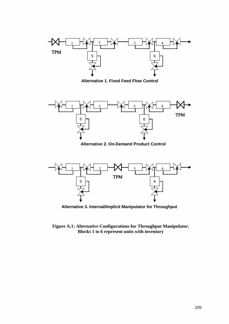
209
Alternative 1. Fixed Feed Flow Control
Alternative 2. On-Demand Product Control
Alternative 3. Internal/Implicit Manipulator for Throughput
1 2 3 4
TPM
1 2 3 4
TPM
5 6
1 2 3 4
TPM5 6
5 6
Alternative 1. Fixed Feed Flow Control
Alternative 2. On-Demand Product Control
Alternative 3. Internal/Implicit Manipulator for Throughput
1 2 3 4
TPM
1 2 3 41 2 3 4
TPM
1 2 3 4
TPM
1 2 3 41 2 3 4
TPM
55 66
1 2 3 4
TPM5 6
1 2 3 41 2 3 4
TPM55 66
55 66
Figure A.1: Alternative Configurations for Throughput Manipulator. Blocks 1 to 6 represent units with inventory
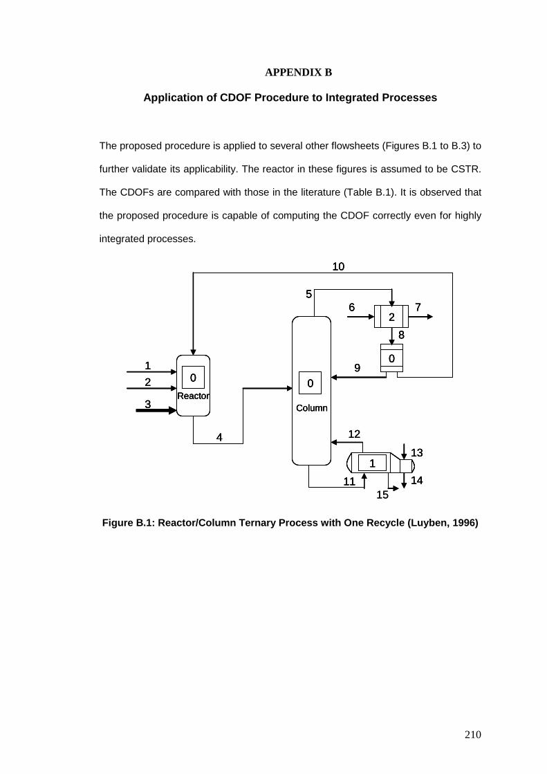
210
APPENDIX B
Application of CDOF Procedure to Integrated Processes
The proposed procedure is applied to several other flowsheets (Figures B.1 to B.3) to
further validate its applicability. The reactor in these figures is assumed to be CSTR.
The CDOFs are compared with those in the literature (Table B.1). It is observed that
the proposed procedure is capable of computing the CDOF correctly even for highly
integrated processes.
1514
13
12
11
ReactorColumn
5
4
1
3
7
10
8
6
92 0 0
1
0
2
1514
13
12
11
ReactorColumn
5
4
1
3
7
10
8
6
92 0 0
1
0
2
14
13
12
11
ReactorColumn
5
4
1
3
7
10
8
6
92 0 0
1
0
2
Figure B.1: Reactor/Column Ternary Process with One Recycle (Luyben, 1996)
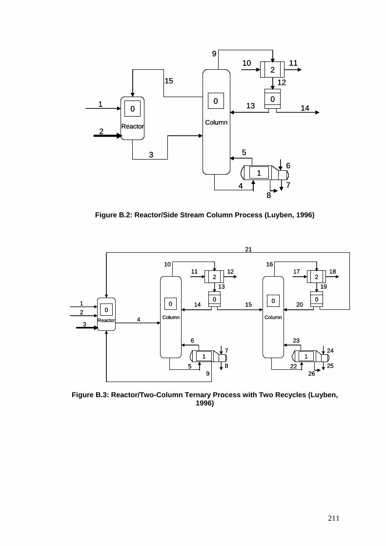
211
7
6
8
5
4
ReactorColumn
9
3
1
2
11
14
12
10
13
15
00
1
2
0
7
6
8
5
4
ReactorColumn
9
3
1
2
11
14
12
10
13
15
00
1
2
0
Figure B.2: Reactor/Side Stream Column Process (Luyben, 1996)
21
8
7
9
6
5
ReactorColumn
10
4
1
3
12
13
11
142
25
24
26
23
22
Column
1618
19
17
201500
0
1 1
2 2
0 0
21
8
7
9
6
5
ReactorColumn
10
4
1
3
12
13
11
142
25
24
26
23
22
Column
1618
19
17
201500
0
1 1
2 2
0 0
Figure B.3: Reactor/Two-Column Ternary Process with Two Recycles (Luyben, 1996)
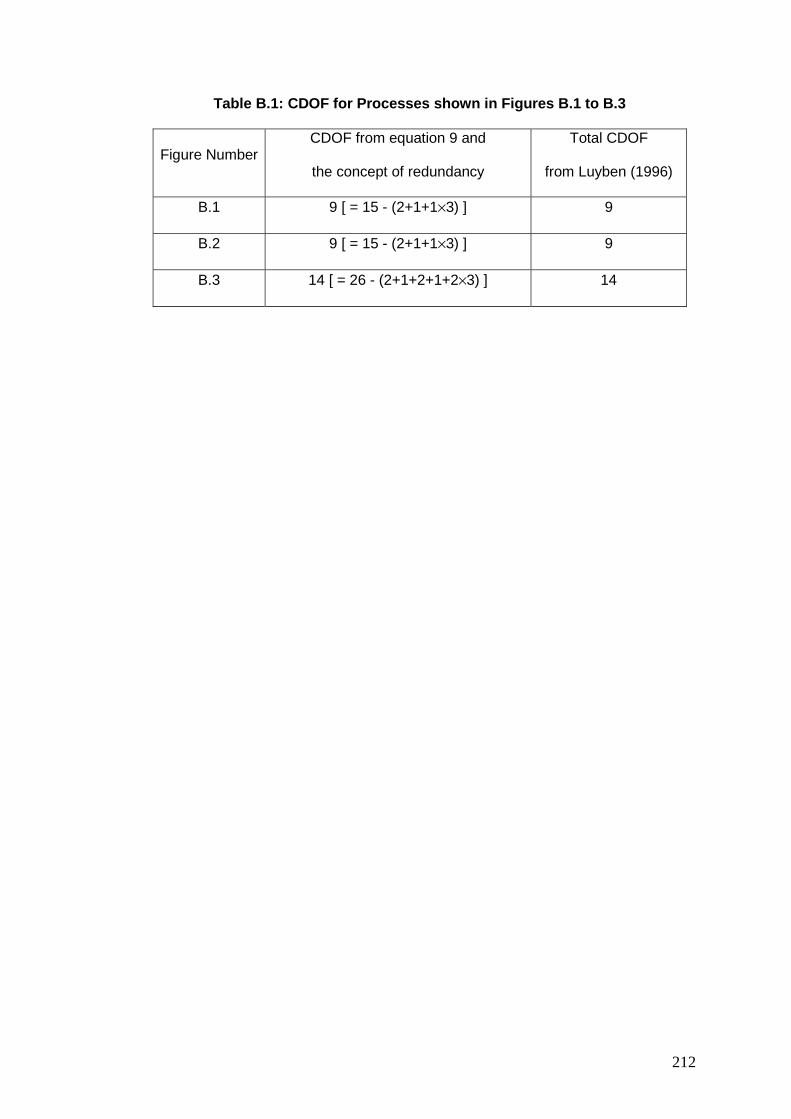
212
Table B.1: CDOF for Processes shown in Figures B.1 to B.3
Figure Number CDOF from equation 9 and
the concept of redundancy
Total CDOF
from Luyben (1996)
B.1 9 [ = 15 - (2+1+1×3) ] 9
B.2 9 [ = 15 - (2+1+1×3) ] 9
B.3 14 [ = 26 - (2+1+2+1+2×3) ] 14
213
APPENDIX C
Resulting Control Structure for Alternative 4 after Step 6 of
Proposed PWC Methodology and Controller Parameters for Alternative 7
Proposed integrated framework is applied to alternative 4 and the resulting
control structure (after step 6 of the procedure) is given in Table C.1. Tuning
parameters for Alternative 7 are given in Table C.2. Flow, pressure and level
controllers are tuned according to Luyben’s (2002) guidelines. Flow controllers are PI
type with a gain of 0.5 and reset time of 0.25 min. Pressure controllers are of the PI
type, with a gain of 2 and reset time 10 min. In general, all level controllers are P-only
type with a proportional gain of either 5 or 10. PI controllers are used for temperature
control, and are tuned using the auto-tuning method with a sensor span of 200 0F.
Composition controllers are also of the PI type and auto-tuning is used to generate
initial values for the controller parameters. If necessary, these controllers are then
fine-tuned to give reasonably good and robust performance, even for the worst-case
disturbance.
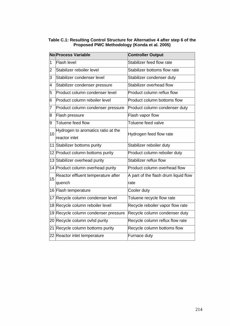
214
Table C.1: Resulting Control Structure for Alternative 4 after step 6 of the Proposed PWC Methodology (Konda et al. 2005)
No Process Variable Controller Output
1 Flash level Stabilizer feed flow rate
2 Stabilizer reboiler level Stabilizer bottoms flow rate
3 Stabilizer condenser level Stabilizer condenser duty
4 Stabilizer condenser pressure Stabilizer overhead flow
5 Product column condenser level Product column reflux flow
6 Product column reboiler level Product column bottoms flow
7 Product column condenser pressure Product column condenser duty
8 Flash pressure Flash vapor flow
9 Toluene feed flow Toluene feed valve
10 Hydrogen to aromatics ratio at the
reactor inlet Hydrogen feed flow rate
11 Stabilizer bottoms purity Stabilizer reboiler duty
12 Product column bottoms purity Product column reboiler duty
13 Stabilizer overhead purity Stabilizer reflux flow
14 Product column overhead purity Product column overhead flow
15 Reactor effluent temperature after
quench
A part of the flash drum liquid flow
rate
16 Flash temperature Cooler duty
17 Recycle column condenser level Toluene recycle flow rate
18 Recycle column reboiler level Recycle reboiler vapor flow rate
19 Recycle column condenser pressure Recycle column condenser duty
20 Recycle column ovhd purity Recycle column reflux flow rate
21 Recycle column bottoms purity Recycle column bottoms flow
22 Reactor inlet temperature Furnace duty
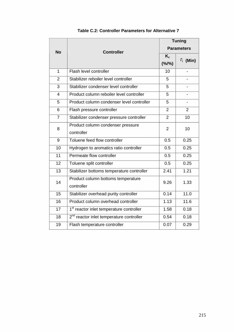
215
Table C.2: Controller Parameters for Alternative 7
Tuning
Parameters No Controller
Kc
(%/%) iτ (Min)
1 Flash level controller 10 -
2 Stabilizer reboiler level controller 5 -
3 Stabilizer condenser level controller 5 -
4 Product column reboiler level controller 5 -
5 Product column condenser level controller 5 -
6 Flash pressure controller 2 2
7 Stabilizer condenser pressure controller 2 10
8 Product column condenser pressure
controller 2 10
9 Toluene feed flow controller 0.5 0.25
10 Hydrogen to aromatics ratio controller 0.5 0.25
11 Permeate flow controller 0.5 0.25
12 Toluene split controller 0.5 0.25
13 Stabilizer bottoms temperature controller 2.41 1.21
14 Product column bottoms temperature
controller 9.26 1.33
15 Stabilizer overhead purity controller 0.14 11.0
16 Product column overhead controller 1.13 11.6
17 1st reactor inlet temperature controller 1.58 0.18
18 2nd reactor inlet temperature controller 0.54 0.18
19 Flash temperature controller 0.07 0.29
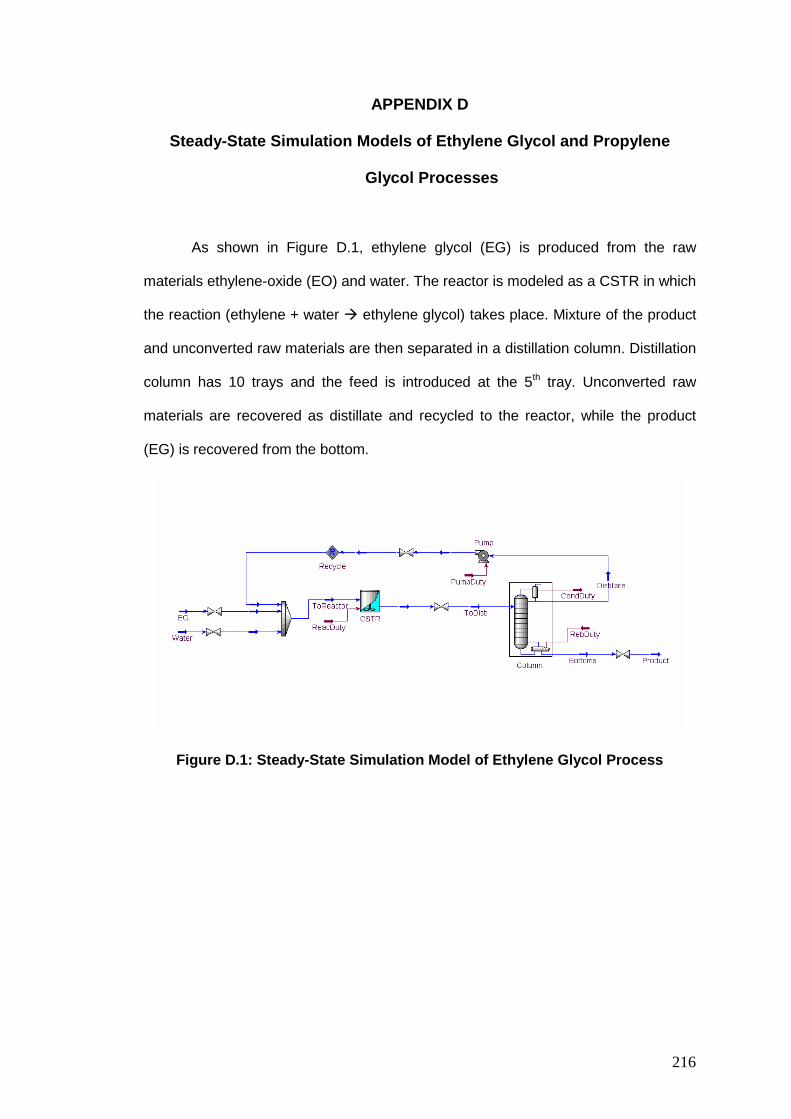
216
APPENDIX D
Steady-State Simulation Models of Ethylene Glycol and Propylene
Glycol Processes
As shown in Figure D.1, ethylene glycol (EG) is produced from the raw
materials ethylene-oxide (EO) and water. The reactor is modeled as a CSTR in which
the reaction (ethylene + water ethylene glycol) takes place. Mixture of the product
and unconverted raw materials are then separated in a distillation column. Distillation
column has 10 trays and the feed is introduced at the 5th tray. Unconverted raw
materials are recovered as distillate and recycled to the reactor, while the product
(EG) is recovered from the bottom.
Figure D.1: Steady-State Simulation Model of Ethylene Glycol Process
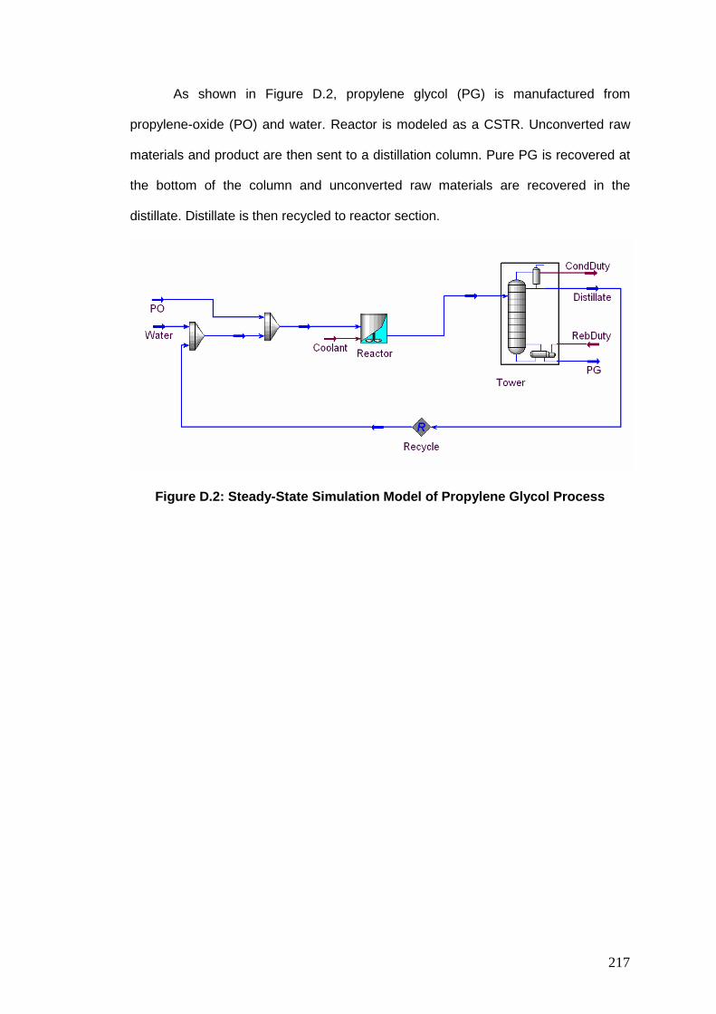
217
As shown in Figure D.2, propylene glycol (PG) is manufactured from
propylene-oxide (PO) and water. Reactor is modeled as a CSTR. Unconverted raw
materials and product are then sent to a distillation column. Pure PG is recovered at
the bottom of the column and unconverted raw materials are recovered in the
distillate. Distillate is then recycled to reactor section.
Figure D.2: Steady-State Simulation Model of Propylene Glycol Process
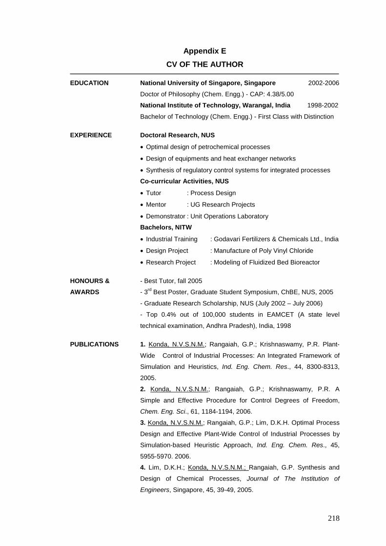
218
Appendix E
CV OF THE AUTHOR
EDUCATION National University of Singapore, Singapore 2002-2006
Doctor of Philosophy (Chem. Engg.) - CAP: 4.38/5.00
National Institute of Technology, Warangal, India 1998-2002
Bachelor of Technology (Chem. Engg.) - First Class with Distinction
EXPERIENCE Doctoral Research, NUS
• Optimal design of petrochemical processes
• Design of equipments and heat exchanger networks
• Synthesis of regulatory control systems for integrated processes
Co-curricular Activities, NUS
• Tutor : Process Design
• Mentor : UG Research Projects
• Demonstrator : Unit Operations Laboratory
Bachelors, NITW
• Industrial Training : Godavari Fertilizers & Chemicals Ltd., India
• Design Project : Manufacture of Poly Vinyl Chloride
• Research Project : Modeling of Fluidized Bed Bioreactor
HONOURS & - Best Tutor, fall 2005
AWARDS - 3rd Best Poster, Graduate Student Symposium, ChBE, NUS, 2005
- Graduate Research Scholarship, NUS (July 2002 – July 2006)
- Top 0.4% out of 100,000 students in EAMCET (A state level
technical examination, Andhra Pradesh), India, 1998
PUBLICATIONS 1. Konda, N.V.S.N.M.; Rangaiah, G.P.; Krishnaswamy, P.R. Plant-
Wide Control of Industrial Processes: An Integrated Framework of
Simulation and Heuristics, Ind. Eng. Chem. Res., 44, 8300-8313,
2005.
2. Konda, N.V.S.N.M.; Rangaiah, G.P.; Krishnaswamy, P.R. A
Simple and Effective Procedure for Control Degrees of Freedom,
Chem. Eng. Sci., 61, 1184-1194, 2006.
3. Konda, N.V.S.N.M.; Rangaiah, G.P.; Lim, D.K.H. Optimal Process
Design and Effective Plant-Wide Control of Industrial Processes by
Simulation-based Heuristic Approach, Ind. Eng. Chem. Res., 45,
5955-5970. 2006.
4. Lim, D.K.H.; Konda, N.V.S.N.M.; Rangaiah, G.P. Synthesis and
Design of Chemical Processes, Journal of The Institution of
Engineers, Singapore, 45, 39-49, 2005.
219
5. Konda, N.V.S.N.M.; Rangaiah, G.P. Performance Assessment of
Plant-Wide Control Systems of Industrial Processes, Ind. Eng. Chem.
Res., 46, 1220-1231. 2007.
6. Zhigui, G.; Konda, N.V.S.N. M.; Rangaiah, G.P. Simulation and
Optimization of a Vinyl Chloride Monomer Plant, submitted to Journal
of The Institution of Engineers, Singapore, June 2006.
PRESENTATIONS 1. Konda, N.V.S.N.M.; Rangaiah, G. P. Performance Assessment of
Plant-Wide Control Systems of Industrial Processes, 11th APCCHE
Congress, Kuala Lumpur, Malaysia, August, 2006.
2. Konda, N.V.S.N.M.; Rangaiah, G. P.; Krishnaswamy, P. R.
Optimal Plant-Wide Design and Control of Industrial Processes, 2nd
Annual Graduate Student Symposium, NUS, Singapore, 2005.
3. Konda, N.V.S.N.M.; Rangaiah, G. P.; Krishnaswamy, P. R.
Simulation based Heuristics Methodology for Plant-Wide Control of
Industrial Processes, 16th IFAC World Congress, Prague, Czech
Republic, 2005.
4. Konda, N.V.S.N.M.; Rangaiah, G. P.; Krishnaswamy, P. R. A
Simple and Effective Procedure for Control Degrees of Freedom, 7th
World Congress of Chemical Engineers, Glasgow, Scotland, 2005.
5. Konda, N.V.S.N.M.; Rangaiah, G. P.; Krishnaswamy, P. R. Plant-
Wide Control of Industrial Processes: An Integrated Framework of
Simulation and Heuristics, 1st Annual Graduate Student Symposium,
NUS, 2004.
6. Konda, N.V.S.N.M.; Rangaiah, G. P.; Krishnaswamy, P. R.
Systematic Classification of Plant-Wide Control System Design
Procedures with Application to the HDA Process, AIChE Annual
Meeting, San Francisco, USA, 2003.
TECHNICAL Basics of Distillation: Design & Simulation, ChBE, NUS, March 2005
TALKS Introduction and Overview of HYSYS, ChBE, NUS, March 2004
EXTRA - General Secretary
CURRICULAR Graduate Students’ Association - ChBE, NUS, 2003 - 2005
ACTIVITIES - Executive member of Technical Committee
Graduate Student Symposium, ChBE, NUS, 2004 & 2005
- Executive member of Organizing Committee
CHEMELIXIR (National Level Symposium), NITW, 2002
- Member of AIChE (2003 – 2004) & IICh


