126
PLASMA GASIFICATION OF ORGANIC WASTE by Nkateko Petra Makaringe © University of Pretoria

PLASMA GASIFICATION OF ORGANIC WASTE
by
Nkateko Petra Makaringe
© University of Pretoria

PLASMA GASIFICATION OF ORGANIC WASTE
by
Nkateko Petra Makaringe
Submitted in partial fulfilment of the requirements for the degree Master of Science
(Applied Science: Chemical Technology)
Department of Chemical Engineering
Faculty of Engineering, Built Environment and Information Technology
UNIVERSITY OF PRETORIA
Supervisor
Prof. P.L. Crouse
Co-supervisors
Dr I.J. van der Walt and Dr M.D.S. Lekgoathi
February 2017
© University of Pretoria

ii
DECLARATION
I, the undersigned, declare that the dissertation, which I hereby submit for the degree Master
of Science in Applied Science: Chemical Technology at the University of Pretoria, is my own
work and has not previously been submitted by me for a degree at any other university.
…………………………… ……………………….
Signature Date
© University of Pretoria

iii
DEDICATION
This work is dedicated to my first born son Xihlovo Makaringe. When I found out I was
pregnant with you I had just started my MSc degree, but I told myself I was going to finish it
no matter how long it took. I want you to follow in your mother’s footsteps. In our language
there is a saying that says: “Dyondzo i xitlhangu xa vutomi”, translating “Education is a
weapon of life”. For as long as you can, I want you to study and equip yourself with education.
You were my inspiration to complete this degree. I wanted to be a good example to you, Son.
I want you to learn to always complete what you have started. And stay positive at all times. I
love you always.
To my late mother; it is unfortunate that you couldn’t see me graduate for the first time for my
National Diploma and you still cannot see me now graduating for MSc. I thank you for paving
an educational way for me. Thank you for taking me to school and for teaching me the value
of education. I swore to make you proud then and I will continue to make you proud even when
you are no longer with us. Everything I do I do it to make you proud. I know if you were still
alive you would be very proud of my achievements. Thank you, Mama. You will always be in
my heart.
© University of Pretoria

SYNOPSIS
iv
PLASMA GASIFICATION OF ORGANIC WASTE
Four biomass materials, namely peach pips, pine wood, bamboo and Napier grass, and one
example of chemical waste, lithium hexafluorophosphate (LiPF6), were studied. The biomass
types were selected because they were easily accessible locally. The LiPF6 waste is solidified
in poly(methyl methacrylate) (PMMA). Gasification of this solid is of interest to industry.
Prior to the gasification studies, TGA-FTRI analyses were conducted on the biomass samples.
This was done to study their thermal behaviour under nitrogen as well as under oxygen. The
results indicated that, in general, pyrolysis of biomass takes place in three stages, namely
hydration, active pyrolysis, and passive pyrolysis. These stages occur at different temperatures
depending on the type of biomass as well as the heating rate used. The conversion efficiency
of these materials is increased under oxygen, due to the fact that combustion takes place in the
presence of oxygen, either partially or fully, depending on the amount made available. TGA
results obtained under nitrogen were used to compute the kinetic parameters of each biomass
material.
Because their fluffy nature led to feed problems, bamboo and Napier grass were excluded from
the plasma gasification experiments. Results obtained during the gasification of peach pips and
pine wood indicated that conversion efficiency slightly increases with an increase in
temperature. Feed rate seemed to have minimal effect on both conversion efficiency and gas
concentration; the energy conversion efficiency did, however, improve.
The conversion efficiencies obtained by TGA and by the plasma system, were roughly similar.
Due to the higher temperatures, ~ 1000 ̊ C, of the plasma reactor, the gaseous products obtained
were predominantly carbon monoxide and hydrogen. On the other hand, carbon dioxide
predominated in the TGA-FTIR experiments. Only a slight trace of monoxide was observed.
Plasma treatment of PMMA encapsulated waste LiPF6 also yielded carbon monoxide and
hydrogen as main products.
The energy conversion efficiency observed for the plasma process was 30 – 40 %. This value
is ratio of the combustion enthalpy of syngas yield and the electrical energy input into the
plasma torch. The main heat loss was via the torch anode. This may be corrected by an
improved thermo-mechanical design.
© University of Pretoria

v
ACKNOWLEDGEMENTS
First and foremost I would like to thank my employer, Necsa, for giving me the opportunity to
further my studies while employed full time. Thank you for supplying the resources that I used
to carry out this work. To Dr I.J. van der Walt, Necsa, thank you for believing in me even when
I didn’t believe in myself. You took me under your wings before I even had my diploma. You
encouraged me to study further and you supported me throughout my studies. I gratefully
appreciate you as my mentor and supervisor.
I am also very thankful to my supervisor, Prof. P.L. Crouse. Firstly thank you for your financial
support through your Chair: Fluoro-Materials Science and Process Integration. Secondly thank
you for your guidance, advice and encouragement throughout my studies from the time I was
doing my honours degree. Lastly I just want to say thank you for your patience. You never
gave up on me, you gave me time to prove myself to you, you continued funding my studies
and I appreciate that a lot.
To Dr M.D.S. Lekgoathi, you are such an inspiration to me, I thank you for your words of
encouragements and for helping me perform some of the experiments here. Mr Cliff
Thompson, you are a blessing to my career. I thank you for your unconditional support. I would
like to thank my colleagues (Jim Sekwaleng, Lesego Wakhaba, Pulane Motau, Piet Scheepers
and Anton Willemse) and staff from Pelindaba Analytical Laboratories. I thank Tando Kili and
Gerard Puts from University of Pretoria. Finally, to my family and friends, thank you for your
support throughout my studies. I thank you all and may God bless you.
© University of Pretoria

vi
LIST OF ABBREVIATION
α Extent of conversion
β Heating rate
AC Alternating current
CFD Computation fluid dynamics
DC Direct current
DTA Differential thermal analysis
DTG Differential thermogravimetric
DSC Differential scanning calorimetric
ER Equivalence ratio
FTIR Fourier transform infrared
GC Gas chromatograph
HHV Higher heating value
LHV Low heating value
MHV Medium heating value
PAL Pelindaba Analytical Laboratories
PMMA Poly(methyl methacrylate)
RF Radio frequency
SSD Sum of square of the difference
Syngas Synthesis gas
TGA Thermogravimetric analysis
© University of Pretoria

vii
TABLE OF CONTENTS
1 Introduction ...................................................................................................................... 14
2 Literature survey ............................................................................................................... 17
2.1 Pyrolysis .................................................................................................................... 17
2.2 Gasification ............................................................................................................... 17
2.2.1 Advantages of gasification processes ................................................................ 18
2.2.2 Types of gasifiers ............................................................................................... 18
2.2.3 Plasma Technology ............................................................................................ 22
2.3 Gasification producer gas .......................................................................................... 27
2.3.1 Tar in a gasification product .............................................................................. 29
2.4 Organic materials ...................................................................................................... 31
2.4.1 Biomass .............................................................................................................. 31
2.4.2 The major components of biomass .................................................................... 31
2.4.3 Biomass characterisation ................................................................................... 33
2.4.5 Composition of selected biomass types used in this study found in literature .. 36
2.4.6 Biomass thermal characterisation ...................................................................... 36
3 Description of experimental equipment ........................................................................... 39
3.1 TGA-FTIR instrument............................................................................................... 39
3.2 Plasma gasification system........................................................................................ 40
3.2.1 Plasma reactor .................................................................................................... 40
3.2.2 Knockout vessel ................................................................................................. 43
3.2.3 Filter ................................................................................................................... 44
3.2.4 Gas sampling point ............................................................................................ 45
4 TGA experiments ............................................................................................................. 46
4.1 Materials .................................................................................................................... 46
4.2 Sample preparation .................................................................................................... 46
© University of Pretoria

viii
4.3 Thermogravimetric analysis ...................................................................................... 46
4.4 Results and discussion ............................................................................................... 47
4.4.1 Pyrolysis under nitrogen .................................................................................... 47
4.4.2 Oxygen atmospheres .......................................................................................... 57
4.4.3 Kinetic model development ............................................................................... 64
4.5 Conclusion ................................................................................................................. 75
5 Plasma gasification experiments ...................................................................................... 76
5.1 Method ...................................................................................................................... 76
5.1.1 Material preparation ........................................................................................... 76
5.1.2 Ultimate analysis ................................................................................................ 77
5.1.3 Screw Feeder calibration.................................................................................... 77
5.1.4 Leak testing ........................................................................................................ 79
5.1.5 Plasma power supply start up ............................................................................ 79
5.1.6 biomass feeding ................................................................................................. 80
5.1.7 Syngas sampling ................................................................................................ 80
5.1.8 Gasification experimental procedure ................................................................. 80
5.2 Results and discussions ............................................................................................. 83
5.2.1 Effect of gasification temperature ...................................................................... 83
5.2.2 Effect of feed rate............................................................................................... 87
5.2.3 Effect of equivalence ratio ................................................................................. 90
5.3 Conclusion ................................................................................................................. 93
6 Conclusion and recommendations .................................................................................... 95
7 Future work: organic chemical waste plasma gasification ............................................... 97
7.1 Chemical waste plasma treatment (LIPF6) ................................................................ 97
7.1.1 Brief background on Lithium hexafluorophosphate .......................................... 97
7.1.2 Waste solidification process .............................................................................. 98
© University of Pretoria
ix
7.1.3 experimental method .......................................................................................... 98
7.1.4 Results and discussions ...................................................................................... 98
7.1.5 Conclusion ......................................................................................................... 99
8 References ...................................................................................................................... 100
Appendices ............................................................................................................................. 107
© University of Pretoria

x
List of Figures
Figure 1. Moving bed (Phillips, 2006) ..................................................................................... 19
Figure 2. Fluidized bed gasifier (Phillips, 2006) ..................................................................... 20
Figure 3. Entrained flow gasifier (Phillips, 2006) ................................................................... 20
Figure 4. Plasma gasifier.......................................................................................................... 21
Figure 5. Various ways of organization plasma gasification (Popov et al., 2011) .................. 22
Figure 6. Four states of matter ................................................................................................. 23
Figure 7. DC transferred arc plasma torch (Gomez et al., 2009) ............................................. 25
Figure 8. DC non-transferred arc plasma torch (Gomez et al., 2009) ..................................... 25
Figure 9. Basic arc operating modes (Duan and Heberlein, 2002) .......................................... 26
Figure 10. Syngas application (Bridgwater, 2003) .................................................................. 29
Figure 11. Tar reduction concept by secondary method (Devi et al., 2003)............................ 30
Figure 12. Tar reduction concept by primary method (Devi et al., 2003) ............................... 30
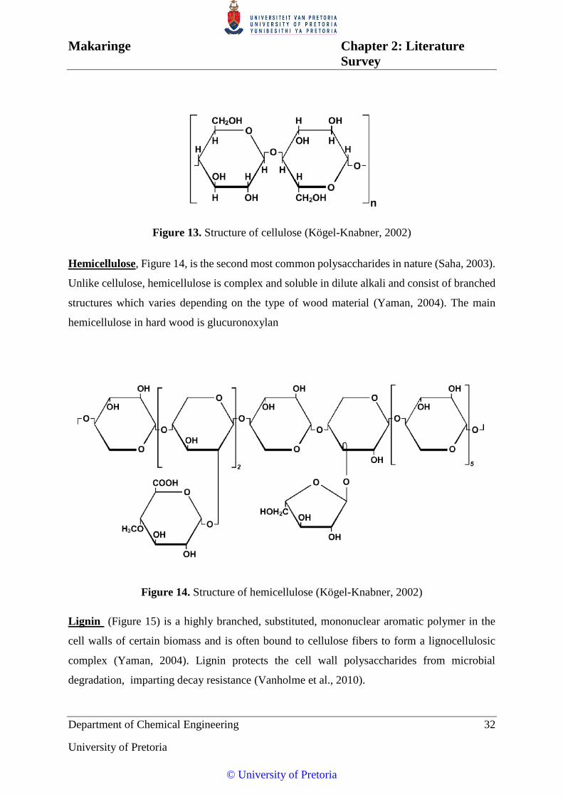
Figure 13. Structure of cellulose (Kögel-Knabner, 2002) ....................................................... 32
Figure 14. Structure of hemicellulose (Kögel-Knabner, 2002) ............................................... 32
Figure 15. Structure of lignin (Kögel-Knabner, 2002) ............................................................ 33
Figure 16. TGA curve of a general biomass sample in the absence of air (Reed et al., 1988)
.................................................................................................................................................. 38
Figure 17. PerkinElmer TGA-FTIR instrument....................................................................... 39
Figure 18. Laboratory scale plasma gasification system ........................................................ 40
Figure 19. Plasma gasification reactor ..................................................................................... 41
Figure 20. Plasma torch ........................................................................................................... 41
Figure 21. A 30 KW plasma power supply.............................................................................. 42
Figure 22. Quench probe.......................................................................................................... 42
Figure 23. Feeding hopper ....................................................................................................... 43
Figure 24. Knockout vessel...................................................................................................... 44
Figure 25. Filter ....................................................................................................................... 45
Figure 26. U-tube ..................................................................................................................... 45
Figure 27. TGA curves of bamboo at 20, 100 and 200 °C/min under nitrogen. ..................... 47
Figure 28. First mass derivative (DTG) curves of bamboo heated at 20, 100 and 200 °C/min
under nitrogen. ......................................................................................................................... 48
Figure 29. Typical TGA and DTG analysis for biomass material (Gašparovič et al., 2010). . 48
© University of Pretoria

xi
Figure 30. FTIR spectra of bamboo heated at 20 °C/min under nitrogen. .............................. 52
Figure 31. FTIR spectra for bamboo heated at 100°C/min under nitrogen. ............................ 53
Figure 32. FTIR spectra of bamboo heated at 200°C/min under nitrogen. ............................. 54
Figure 33. TGA of Napier grass, pine wood, bamboo and peach pips heated at 200 °C/min
under nitrogen. ......................................................................................................................... 56
Figure 34. DTG of Napier grass, pine wood, bamboo and peach pips heated at 200 °C/min
under nitrogen. ......................................................................................................................... 56
Figure 35. TGA of Napier grass, pine wood, bamboo and peach pips at a heating rate of 200
°C/min under oxygen. .............................................................................................................. 58
Figure 36. DTG of Napier grass, pine wood, bamboo and peach pips at a heating rate of 200
°C/min under oxygen. .............................................................................................................. 58
Figure 37. FTIR spectra of bamboo at a heating rate of 200 °C/min under oxygen. ............... 60
Figure 38. FTIR of pine wood at 200°C/min under oxygen. ................................................... 61
Figure 39. FTIR spectra of Napier grass at a heating rate of 200°C/min under oxygen. ........ 62
Figure 40. FTIR spectra of peach pips at a heating rate of 200°C/min under oxygen............. 63
Figure 41. Experimental and predicted α-T curves of peach pips at a heating rate of 200 °C/min
under nitrogen atmospheres. .................................................................................................... 71
Figure 42. Experimental and predicted α-T curves of Napier grass at a heating rate of 200
°C/min under nitrogen. ............................................................................................................ 72
Figure 43. Experimental and predicted α-T curves of pine wood at a heating rate of 200 °C/min
under nitrogen. ......................................................................................................................... 73
Figure 44. Experimental and predicted α-T curves of bamboo at a heating rate of 200 °C/min
under nitrogen. ......................................................................................................................... 74
Figure 45. Pine wood chips ...................................................................................................... 76
Figure 46. Peach pips ............................................................................................................... 76
Figure 47. Screw feeder calibration curve for pine wood chips .............................................. 78
Figure 48. Screw feeder calibration curve for peach pips ....................................................... 78
Figure 49. The equivalence ratio diagram (Reed and Desrosiers) ........................................... 82
Figure 50.Temperature vs conversion using peach pips as feed .............................................. 84
Figure 51. Product yield vs temperature using peach pips ...................................................... 85
Figure 52. Feed rate vs conversion curve ................................................................................ 88
Figure 53. Product yield vs feed rate using peach pips as feed ............................................... 89
© University of Pretoria

xii
Figure 54. Pine wood conversion vs ER .................................................................................. 91
Figure 55. Product yield vs ER ................................................................................................ 92
Figure 56. PMMA encapsulated waste .................................................................................... 98
Figure 57. TGA curve of pine wood under nitrogen ............................................................. 107
Figure 58. DTG curve of pine wood under nitrogen. ............................................................ 107
Figure 59. FTIR spectra of pine wood at 100°C/min under nitrogen. ................................... 108
Figure 60. TGA curves of Napier grass under nitrogen......................................................... 109
Figure 61. DTG curve of Napier grass under nitrogen. ......................................................... 109
Figure 62. FTIR spectra of Napier grass at 20°C/min under nitrogen. .................................. 110
Figure 63. FTIR spectra of Napier grass at 100°C/min under nitrogen. ................................ 111
Figure 64. TGA curves of peach pips under nitrogen ............................................................ 112
Figure 65. DTG curve of peach pips under nitrogen. ............................................................ 112
Figure 66. FTIR spectra of peach pips at 20°C/min under nitrogen. ..................................... 113
Figure 67. FTIR spectra of peach pips at 100°C/min under nitrogen. ................................... 114
Figure 68. TGA curve of pine wood under oxygen. .............................................................. 115
Figure 69. DTG curve of pine wood under oxygen. .............................................................. 115
Figure 70. FTIR spectra of pine wood at 20°C/min under oxygen. ....................................... 116
Figure 71. FTIR spectra of pine wood at 100°C/min under oxygen. ..................................... 117
Figure 72. TGA curve of Napier grass under oxygen. ........................................................... 118
Figure 73. DTG curve of Napier grass under oxygen. ........................................................... 118
Figure 74. FTIR spectra of Napier grass at 20°C/min under oxygen. ................................... 119
Figure 75. FTIR spectra of Napier grass at 100°C/min under oxygen. ................................. 120
Figure 76. FTIR spectra of Napier grass at 200°C/min under oxygen. ................................. 121
Figure 77. TGA curve of peach pips under oxygen. .............................................................. 122
Figure 78. DTG curve of peach pips under oxygen. .............................................................. 122
Figure 79. FTIR spectra of peach pips at 20°C/min under oxygen. ...................................... 123
Figure 80. FTIR spectra of peach pips at 100°C/min under oxygen. .................................... 124
Figure 81. FTIR spectra of peach pips at 200°C/min under oxygen. .................................... 125
© University of Pretoria

xiii
List of Tables
Table 1. Typical product weight yield (dry wood basis) obtained by different modes of
pyrolysis of wood (Bridgwater, 2012) ..................................................................................... 17
Table 2. Methods of biomass fuel analyses (Demirbas, 2004) ................................................ 34
Table 3. Proximate analysis of typical biomass material (wt %) ............................................. 35
Table 4. Ultimate analysis of typical biomass material (wt %) ............................................... 35
Table 5. Calorific value of typical biomass material (MJ/kg) ................................................. 35
Table 6. Proximate analysis of selected biomass material ....................................................... 36
Table 7.Ultimate analysis of biomass material used in this study ........................................... 36
Table 8. Kinetic model parameters for the thermal decomposition of peach pips. ................. 67
Table 9. Kinetic model parameters for the thermal decomposition of Napier grass. .............. 68
Table 10. Kinetic model parameters for the thermal decomposition of pine wood. ................ 69
Table 11. Kinetic model parameters for the thermal decomposition of bamboo..................... 70
Table 12. Ultimate analysis of four biomass material (molar %) ............................................ 77
Table 13. Plasma power supply start up procedure ................................................................. 79
Table 14. Calorific value of syngas produced from gasification of peach pips at different
temperatures ............................................................................................................................. 86
Table 15: Average power losses to various water-cooled torch and reactor components ....... 87
Table 16. Calorific values of syngas produced from gasification of peach pips at different feed
rates .......................................................................................................................................... 90
Table 17 Calorific values of syngas produced for gasification of pine wood at different ER . 93
© University of Pretoria

Department of Chemical Engineering 14
University of Pretoria
1 INTRODUCTION
Waste generation has been increasing significantly due to an increase in population and urban
and industrial development worldwide. By 1998 waste generated in South Africa only had risen
to 533 million tonnes per annum (Nahman et al., 2012). The generation of waste in South
Africa is expected to increase as a result of population and economic growth at a predicted rate
of 2-3% per annum (Nahman et al., 2012). Due to this increase in waste, there is an increased
demand of waste services in terms of collection, transportation, storage, handling and
treatment.
On the other hand, due to the increase in population, the energy demand is also increasing. The
fossil fuels such as coal are primarily used for the production of energy worldwide. Though
coal is available in abundance in countries like United State of America and Russia, resources
are declining at an alarming rate due to high energy demand. Eventually the worldwide
supplies of these fossil fuels will be exhausted.
Climate change is a major environmental problem. Carbon dioxide (CO2) emission is the main
concern when using fossil fuel as a source of energy. Concentration of CO2 in the atmosphere
will continue to rise unless major changes are made in the way fossil fuels are used to provide
energy services (Berndes et al., 2003). As a solution to CO2 emission problem, there is a call
for greenhouse gas concentrations to remain at a level that would prevent dangerous
anthropogenic interference with climate system (Berndes et al., 2003). As a response to this
call, other cleaner sources of energy are being explored. Nuclear energy is a popular choice,
but there are major safety concerns with nuclear.
Biofuel and energy from organic waste is a recent development. It serves as a waste treatment
technology and clean energy solution while in turn closing the energy demand gap. Organic
waste is gasified to produce synthesis gas which can either be converted to electricity or
converted to biofuel through the Fischer-Tropsch process. Incineration is amongst other
methods conventionally used for waste treatment (Tendler et al., 2005). However it results in
the formation of tar and char which need further treatment (Gassner and Maréchal, 2009).
Thermal plasma gasification is an innovative process for the waste treatment which seems to
have distinct advantages.
© University of Pretoria
Makaringe Chapter 1: Introduction
Department of Chemical Engineering 15
University of Pretoria
This is due to the high temperatures found in plasma systems. In a plasma gasification process,
the organic compounds are thermally decomposed into their constituent elements and
converted into synthetic gas (syngas), which consists mainly of hydrogen (H2) and carbon
monoxide (CO) (Galeno et al., 2011). The inorganic materials are melted and converted into a
dense, inert, non-leachable vitrified slag.
Necsa is in the process of developing such process for organic waste plasma gasification for
the production of syngas, which will be further used for electricity generation. The
effectiveness of this process depends on the quality of syngas, which in turn depends on the
gasification process.
A laboratory scale organic waste plasma gasification system is currently used as a research
facility by Necsa. The data collected during the series of experimental tests will be used as
input into the design of the syngas production facilities. There are number of problems
encountered during the operation of this laboratory system. One main problems is the carbon
residues remaining after every experimental run which lead to the system having downtime for
maintenance (mainly for the removal of carbon residues from the reactor, pipes and traps). The
second main problem is the fluctuation in the gas yields. The ideal gas composition for the
gasification process is to achieve high CO and H2 yield with minimum CO2, tar, carbon residues
and CH4. This has not been optimised.
The objective of this study was to investigate deferent parameters such as feed rate, operating
temperatures, equivalence ratios, etc., which have direct influence in the quality of syngas
produced and tar formation during biomass plasma gasification processes. The optimum
parameters which will give high quality syngas product and no tar will be used when up scaling
the system.
Different types of biomass behave differently when gasified. Therefore it was thought to be
important to characterise each material used as a feed during gasification process. Hence this
study was divided into two sections. The first part comprises the characterisation of four
different biomass materials. Here the reaction rates of the materials were studied using
thermogravimetric analysis (TGA).
The second part of the study was to study the operating parameters of a laboratory scale organic
waste plasma gasification reactor. This included gasification experiments on four types of
© University of Pretoria

Makaringe Chapter 1: Introduction
Department of Chemical Engineering 16
University of Pretoria
biomass (viz. peach pips, pine wood, bamboo and Napier grass) as well as performing a
preliminary gasification study on chemical waste. The chemical waste was scrap lithium
hexafluolrophosphate (LiPF6), embedded in poly(methyl methacrylate (PMMA). The aim here
was to see whether PMMA would yield a significant amount of syngas.
© University of Pretoria

Department of Chemical Engineering 17
University of Pretoria
2 LITERATURE SURVEY
2.1 PYROLYSIS
Pyrolysis is thermal decomposition which occurs in the absence of oxygen (Bridgwater, 2012).
Biomass pyrolysis can result in the production of three products, viz. liquid, solid and gas.
Their proportions can be varied by adjusting the process parameters. The product distributions
from different modes of pyrolysis are shown in Table1.
Table 1. Typical product weight yield (dry wood basis) obtained by different modes of
pyrolysis of wood (Bridgwater, 2012)
Mode Condition Liquid Solid Gas
Fast ~500°C, short hot vapour residence
time ~1 s
75% 12% char 10%
Intermediate ~500°C, hot vapour residence time
~10-30 s
50% in 2 phase 25% char 25%
Carbonisation
(Slow)
~400°C, long vapour residence hours
— days
30% 35% char 35%
Gasification ~750-900°C short hot vapour
residence time- seconds
5% 10% char 85%
Torrefaction
(Slow)
~290°C, solids residence time ~10—
60 min
0% 80% char 20%
2.2 GASIFICATION
Operation of the pyrolysis process in a lean oxygen environment is called gasification.
Gasification is a process in which combustible materials are partially oxidized or partially
combusted(Phillips, 2006). As it can be seen from Table 1, gasification generates 85% gas,
10% solids and 5% liquids when operated at temperatures between 700 and 900 °C. The gases
produced during gasification are combustible synthesis gases, also known as syngas, which can
be further processed to produce chemicals, fertilizers, liquid fuels, hydrogen and electricity
© University of Pretoria

Makaringe Chapter 2: Literature
Survey
Department of Chemical Engineering 18
University of Pretoria
(Rozelle and Der, 2015). Operation of the gasification process in the presence of oxygen
(partial oxidization rather than complete oxidization) increases the yield of these gases and
eliminates/reduces the tar production (Hlina et al., 2011). To achieve near complete conversion
of biomass to syngas, gasification processes are typically operated above their stoichiometric
oxygen-fuel ratio.
2.2.1 ADVANTAGES OF GASIFICATION PROCESSES
Gasification is among the cleanest and most efficient technologies. Less CO2 is emitted during
gasification because there are not enough oxygen atoms available to fully react with the feed
material(Phillips, 2006). In turn instead of producing CO2 (which is an environmental
pollutant), the carbon feed is converted primarily to carbon monoxide (CO), and the hydrogen
in the feed is converted to H2 rather than H2O (Phillips, 2006).
The other advantage of gasification is that a fraction of the heating value (known as a cold gas
efficiency) available in the feed stock remains in the product gas. Due to this, most gasifiers
are operated with no water cooling to minimize heat losses.
As indicate in Table 1, another advantage of gasification is minimum tar yield. It is very
important to have less tar or no tar in the product gas because tar would condense at low
temperatures and lead to clogged or blockage in fuel lines, filters and engines (Han and Kim,
2008).
Different types of gasifiers have been studied and designed with the attempt of exploring these
advantages. Some of these gasifiers are discussed in Section 2.2.2. Plasma gasifiers are of
particular of interest for this study.
2.2.2 TYPES OF GASIFIERS
There are three main types of gasifiers conventionally applied in coal gasification processes.
These are moving bed, fluidized bed and entrained flow gasifiers. A brief background of these
gasifiers is given here. There is, however, a constant development of new technologies in order
to achieve, among others things, a simplified, efficient and tar free syngas production system.
These systems can handle a variety of feed stock such as biomass, municipal waste, medical
waste, and so on. Plasma gasification is an example of a recently developed technology and is
© University of Pretoria

Makaringe Chapter 2: Literature
Survey
Department of Chemical Engineering 19
University of Pretoria
discussed here as of primary interest.
2.2.2.1 MOVING BED
A moving bed gasifier is a countercurrent flow reactor where the feed stock (in the form of
large particles and fluxes) is loaded from the top of the gasifier and moves slowly downwards
through the bed while reacting with oxygen containing gas which is introduced at the bottom
(Figure 1). The remaining ash after gasification drops out at the bottom of the reactor. In a
moving bed gasifier, the reaction happens in 4 stages, namely the drying zone at the top of the
reactor, the carbonization zone, the gasification zone, and lastly the combustion zone at the
bottom of the reactor.
Figure 1. Moving bed (Phillips, 2006)
2.2.2.2 FLUIDIZED BED
A fluidized bed gasifier is one of the most frequently used gasification rectors
(Meng et al., 2011). They have excellent heat and mass transfer between the gas and the solid
phases with the best temperature distribution throughout the bed created by their back mixing.
The flow of the oxidant into the reactor is sufficient to float the particles, but not too high to
flush the particles out of the bed. The particles size required to sustain the bed is small
(< 6 mm). In a fluidized bed, the feed enters at the side of the reactor while the oxidant enters
at the bottom (near the bottom) with sufficient velocity to fully suspend or fluidize the reactor
bed (Figure 2).
© University of Pretoria

Makaringe Chapter 2: Literature
Survey
Department of Chemical Engineering 20
University of Pretoria
Figure 2. Fluidized bed gasifier (Phillips, 2006)
2.2.2.3 ENTRAINED FLOW
This is a co-current flow reactor where the finely ground feed stock is fed co-currently with the
oxidant from the top of the reactor. Entrained gasifiers operate at high temperatures due to their
short residence time, resulting in a high carbon conversion efficiency. Because of these high
operating temperatures, the syngas produced is tar free and the ashes are melted into vitreous
slag (Figure 3). However, these high temperatures tend to shorten the life of the system
components.
Figure 3. Entrained flow gasifier (Phillips, 2006)
2.2.2.4 PLASMA GASIFIERS
Plasma reactors are known and used for treatment of a wide range of material including scrap
© University of Pretoria

Makaringe Chapter 2: Literature
Survey
Department of Chemical Engineering 21
University of Pretoria
metal, hazardous waste, municipal and industrial waste and landfill material to derive useful
material or to vitrify undesirable waste for easier deposition (Dighe et al., 2010).
In a plasma gasification process electric arc generators (plasmatrons or plasma torches) are
used (Rutberg et al., 2011; Lemmens et al., 2007; Tendler et al., 2005) (Figure 4). Here the arc
(or arcs, in case of multiple torches) is sustained inside a discharge chamber. The plasma flow
is injected into the plasma chemical reactor/gasifier by means of nozzle of various types.
Figure 4. Plasma gasifier
Several plasma gasification configurations, as illustrated in Figure 5, are possible
(Popov et al., 2011).
© University of Pretoria

Makaringe Chapter 2: Literature
Survey
Department of Chemical Engineering 22
University of Pretoria
Figure 5. Various ways of organization plasma gasification (Popov et al., 2011)
Conventionally organic materials are processed using pyrolysis reactors which mostly results
in a formation of tars and production of poor quality syngas. The required tar content for most
syngas application is of the order 0.05 g/m3 or less (Han and Kim, 2008). To improve the
pyrolysis results, plasma reactors have been coupled with pyrolysis reactors
(Luche et al., 2012). The plasma acts as a purification stage by reducing the production of tars
and aerosols, and produces a hydrogen rich syngas. However the pyrolysis reactors could be
eliminated and plasma reactors could be used alone as gasification medium.
In 2006, Europlasma announced a new gasification process which maximizes mass yield from
biomass by using an external source to feed the endothermic reaction.
2.2.3 PLASMA TECHNOLOGY
Plasma technology was used in the sixties primarily for space related activities
(Pfender, 1999; Fauchais and Vardelle, 1997). It gradually transitioned to a well-established
interdisciplinary science with a wide range of important application in material processing in
the eighties (Boulos, 1991). The understanding of interaction between thermal plasmas and
particulates has been researched and has successfully been applied in the areas such as arc
© University of Pretoria

Makaringe Chapter 2: Literature
Survey
Department of Chemical Engineering 23
University of Pretoria
welding, arc cutting, plasma synthesis of fine powders, plasma waste destruction, etc (Pfender,
1999). Adapted from their waste destruction application (Camacho, 1996) the technology has
recently being utilised for their application in biomass gasification due to their high
temperatures and high energy densities along with their corresponding fast reaction times
(Gomez et al., 2009).
2.2.3.1 WHAT IS A PLASMA?
Plasma can be defined as the fourth state of matter (Boulos et al., 2013). The general principle
of physics is that matter changes its state as energy is supplied to it. Solids become liquid, and
liquid become gas. When even more energy is applied to gases, they ionise and become the
energy rich plasma state (Figure 6). Hence it is called the fourth state of matter. A high amount
of energy is needed to produce a plasma. Plasma consists of a mixture of electrons, ions and
neutral species in local electrical neutrality (Boulos, 1991).
Figure 6. Four states of matter
Plasmas of can be divided into two categories: thermal plasmas and non-thermal plasmas.
Thermal plasmas are atmospheric plasmas characterised by high enthalpy content and
temperatures around 2000 – 20000 °C (Venkatramani, 2002). Non-thermal plasmas are low
pressure plasmas characterised by high electron temperatures and low ion and neutral particle
temperatures. Thermal plasmas are widely used for plasma processing and metallurgical
applications. They have recently also found application in biomass gasification processes, as
© University of Pretoria

Makaringe Chapter 2: Literature
Survey
Department of Chemical Engineering 24
University of Pretoria
mentioned above.
2.2.3.2 THERMAL PLASMAS
Thermal plasmas are normally generated by passing an electric current through a gas
(Boulos et al., 2013). This is done in a plasma torch by direct current (DC), alternating current
(AC), radio frequency (RF) and other discharges. The direct current (DC) plasma torches are
widely used and they consist of a water cooled cathode and anode. The two electrodes are
separated by an insulator which has an inlet for a plasma gas. When a plasma gas is introduced
in the electrode gap and a DC arc is established between the electrodes, the arc is pushed
through the anode nozzle resulting in a high temperature high velocity flame. The arc is a self-
sustaining discharge with a voltage drop of a few volts near the electrodes. It is also highly
turbulent. Any disturbance from equilibrium is undesirable since it tend to extinguish the arc
(Venkatramani, 2002).
The features that makes thermal plasma attractive is the high energy density
(~106-107 J/m3) which comes with high heat flux density (~107-109 W/m2), high quenching rate
(~106-108 K/s) and high processing rate (Trelles et al., 2009).
2.2.3.3 PLASMA TORCHES
A plasma torch is a device used to produce thermal plasmas as mentioned earlier. There are
different types and geometries of plasma torches. The two main types of plasma torches are
transferred (Figure 7) and the non-transferred arcs (Figure 8). In a transferred geometry, the
electric arc used to generate the plasma is maintained between one electrode of the torch (the
cathode) and a conductive work piece that needs to be cut or melted (act as anode), located
outside the torch (Favalli and Szente, 1998).
© University of Pretoria

Makaringe Chapter 2: Literature
Survey
Department of Chemical Engineering 25
University of Pretoria
Figure 7. DC transferred arc plasma torch (Gomez et al., 2009)
A non-transferred torch uses two water cooled electrodes (cathode and anode) in order to
maintain the electric arc (Favalli and Szente, 1998). The electric arc strikes between the two
electrodes of the torch and it is kept inside the anode channel.
Figure 8. DC non-transferred arc plasma torch (Gomez et al., 2009)
© University of Pretoria

Makaringe Chapter 2: Literature
Survey
Department of Chemical Engineering 26
University of Pretoria
Today plasma torches are used as unique heating tools in industrial processes. The industrial
application of plasma torches includes waste destruction, experimental gas heating for solving
the issues of aerodynamic heating of re-entry hypersonic vehicles, synthesis of nanostructure
material, plasma chemistry and material deposition (plasma spaying) or removal (plasma
etching) (Venkatramani, 2002; Murphy, 2001).
2.2.3.4 PLASMA ARC
There are three different arc modes of operating the torch that have been identified according
to the voltage fluctuations (Figure 9). They are:
Steady mode
Take-over (quasi-periodic) mode and
Restrike mode
Figure 9. Basic arc operating modes (Duan and Heberlein, 2002)
These modes are described in the order of decreasing current or increasing flow rate. The steady
mode is characterised by a fixed position of the anode attachment and negligible voltage
fluctuation. The take-over mode is characterised by a periodic or quasi-periodic movement of
the arc and fluctuating voltage while the restrike mode is characterised by the highly unstable,
unpredictable movement of the arc and quasi-chaotic fluctuation of the voltage (Duan and
© University of Pretoria

Makaringe Chapter 2: Literature
Survey
Department of Chemical Engineering 27
University of Pretoria
Heberlein, 2002).
The ideal movement of the arc is the quasi-periodic movement with high frequency and small
amplitude as in a take-over mode. This allows uniform distribution of the thermal load over the
anode while forcing the jet homogenously (Trelles et al., 2006)
In a non-transferred arc plasma torch, the fluctuation behaviour of the arc may negatively affect
the process. In plasma torches which are used for thermal spraying it may lead to a non-uniform
heating of the injected powder particles (Dorier et al, 1999). This may negatively affect the
quality and yield of the spray deposits. Plasma torches used for material processing and waste
destructions are similar to the one used for thermal spraying (Favalli & Szente, 1998), the
difference being the exclusion of the powder inlet, hence the fluctuation behaviour of the arc
will have the same effects.
For transfer arc plasma torches, the process is characterised by a transferred electric arc that is
established between the cathode and the anode (molten metallic work piece). In order to
achieve a high quality and high productivity process, a plasma jet must be as collimated as
possible and must have a higher achievable power density (Colombo et al, 2009). The
fluctuation behaviour of the arc will therefore have an effect on the plasma jet.
In order to obtain design strategies to achieve the quasi-periodic movement of the arc
(which result is a less fluctuating arc), a better understanding of the processes driving the
dynamics of the arc inside the torch is required. The dynamics of the arc inside the plasma
torch is a result of the balance between the drag force caused by the interaction of the incoming
gas flow over the arc and the electromagnetic Lorentz forces caused by the local curvature of
the arc (Trelles et al, 2006). Computational fluid dynamics (CFD) is used as a tool in many
studies for a better understanding of the dynamics of plasma arcs (Klinger et al., 2003; Meng
and Dong, 2011; Reynolds et al., 2010; Trelles et al., 2009).
2.3 GASIFICATION PRODUCER GAS
Synthesis gas (syngas) is the main product of the gasification process. It consists mainly of
hydrogen (H2) and carbon monoxide (CO). Traces of hydrocarbons such as methane are also
found in a gasification product gas (Bridgwater, 2003). The H2 and CO are produced during
gasification according to the following reactions:
© University of Pretoria

Makaringe Chapter 2: Literature
Survey
Department of Chemical Engineering 28
University of Pretoria
22 HCOOHC 1
222 HCOOHCO 2
422 CHHC 3
222
1HyxxCOOxHHC YX
4
COCOC 22 5
The most important reaction is Equation 5 known as Boudouard reaction. In this reaction
carbon converts CO2 to CO (one of the primary products of gasification) (Lemmens et al.,
2007). It is of high interest to achieve low CO2 emission since it is of no value in syngas and it
is a pollution hazard. A high CO/CO2 ratio is achieved at high temperatures and it is considered
an important parameter for control of the gasification process (Lemmens et al., 2007)).
As mentioned in Section 2.2, gasification occurs in an oxygen starved environment. This also
prevents the formation CO2 since there are not enough oxygen atoms to react with the feed.
Therefore the precise amount of oxygen as a reagent also plays an important role in the
composition of the syngas.
Pure O2, air, steam, CO2, H2 or a mixture of these could be used as reagents
(Puig-Arnavat et al., 2010). When oxygen is used as a reagent a high quality syngas with a
medium heating value (MHV) of ~10-12 MJ/m3 (Bridgwater, 2003; McKendry, 2002b) is
produced. However the use of air introduces the presence of nitrogen in the final product which
reduces the quality of the gas which in turn results in a low heating value (LHV) of ~5 MJ/m3
(Bridgwater, 2003; McKendry, 2002b; Rutberg et al., 2011). Higher heating value (HHV) of
up to 40 MJ/m3 is usually achieved when hydrogen is used as a reagent (McKendry, 2002b).
This is presented in Figure 10.
© University of Pretoria

Makaringe Chapter 2: Literature
Survey
Department of Chemical Engineering 29
University of Pretoria
Figure 10. Syngas application (Bridgwater, 2003)
The storage or transportation of gas is very costly, therefore it has to be used immediately after
production. Low heating value gas is used directly in combustion or as an engine fuel to
produce electricity while medium heating value gas is used as a feedstock for conversion into
other products such as liquid hydrocarbons.
2.3.1 TAR IN A GASIFICATION PRODUCT
Tar formation during the gasification process is one of the main problems to be dealt with.
Higher molecular weight compounds in the product gas begin to condense at temperatures
below 450 °C and form tar (McKendry, 2002b) . The presence of tar in a syngas can be
problematic because it can result in blocking and fouling of process equipment (Chen et al.,
2003). It also hinders the process of removing the particulates from the gas.
Hot gas cleaning after the gasifier is the less preferred tar removal process
(Figure 11). Two methods for tar removal are catalytic cracking using dolomite or nickel, and
thermal cracking by partial oxidation or direct contact (Bridgwater, 2003; Chen et al., 2003).
The use of CO2 with a catalyst like Ni/Al as a gasifying agent could also be beneficial for tar
reduction as it can transform char, tar and CH4 into H2 and CO
© University of Pretoria

Makaringe Chapter 2: Literature
Survey
Department of Chemical Engineering 30
University of Pretoria
(Puig-Arnavat et al., 2010).
Figure 11. Tar reduction concept by secondary method (Devi et al., 2003)
Tar treatment inside the gasifier is the primary and most preferred method (Figure 12). It
eliminates the secondary tar treatment methods during gasification processes. The operating
parameters such as temperatures, feeding rate, gasifying reagent, equivalence ratio, residence
time, etc., play an important role in the formation and decomposition of tar inside a gasifier
(Dufour et al., 2009; Guo et al., 2014; Berrueco et al., 2015a).
Figure 12. Tar reduction concept by primary method (Devi et al., 2003)
In order to get the best quality, tar free syngas, the design and the operation of the gasifier has
to be optimised.
© University of Pretoria

Makaringe Chapter 2: Literature
Survey
Department of Chemical Engineering 31
University of Pretoria
2.4 ORGANIC MATERIALS
Carbon containing compounds are generally defined as organic materials in modern chemistry.
Organic compound are predominantly combinations of hydrogen, carbon, nitrogen, and
oxygen. Organic materials include the wood, feathers, leather, synthetic materials such as
plastics and many more.
2.4.1 BIOMASS
Apart from being defined as organic material, biomass can also be defined as a renewable,
storable and transportable energy source. It is available in different forms, such as wood,
agricultural and forest residues, and garbage. Biomass consist of organic components such as
hemicellulose, cellulose, lignin, lipids, proteins, starches and sugars. It also contains water,
alkaline and alkaline earth metals, chlorine, nitrogen, phosphorous, sulphur, silicon and heavy
metals.
2.4.2 THE MAJOR COMPONENTS OF BIOMASS
Hemicelluloses, cellulose and lignin are the three major components of biomass and they
generally cover 20-40, 40-60, and 10-25 wt % of lignocellulosic biomass respectively (Yang
et al., 2007).
Cellulose is a polysaccharide with a general formula of (C6H10O5)n and average molecular
weight of 300 000 – 500 000 g/mol (Yaman, 2004). The structural formula is shown in
Figure 13. Cellulose is insoluble in water and forms the skeletal structure of most biomass. It
is the most abundant natural polymer on earth, consisting of glucose-glucose linkages arranged
in linear chains where every other glucose residue is rotated in the opposite direction (Kim et
al., 2006). The yearly biomass production of cellulose is estimated to be 1.5 trillion tons (Kim
et al., 2006). Starch and cotton are examples of cellulose.
© University of Pretoria
Makaringe Chapter 2: Literature
Survey
Department of Chemical Engineering 32
University of Pretoria
Figure 13. Structure of cellulose (Kögel-Knabner, 2002)
Hemicellulose, Figure 14, is the second most common polysaccharides in nature (Saha, 2003).
Unlike cellulose, hemicellulose is complex and soluble in dilute alkali and consist of branched
structures which varies depending on the type of wood material (Yaman, 2004). The main
hemicellulose in hard wood is glucuronoxylan
Figure 14. Structure of hemicellulose (Kögel-Knabner, 2002)
Lignin (Figure 15) is a highly branched, substituted, mononuclear aromatic polymer in the
cell walls of certain biomass and is often bound to cellulose fibers to form a lignocellulosic
complex (Yaman, 2004). Lignin protects the cell wall polysaccharides from microbial
degradation, imparting decay resistance (Vanholme et al., 2010).
© University of Pretoria

Makaringe Chapter 2: Literature
Survey
Department of Chemical Engineering 33
University of Pretoria
Figure 15. Structure of lignin (Kögel-Knabner, 2002)
2.4.3 BIOMASS CHARACTERISATION
Biomass characteristics such as heating value, moisture and ash contents as well as elemental
composition has a significant effect on the design and operation of gasifying systems
(Yin, 2011). Table 2 below shows the ASTM methods used to analyse these biomass
properties.
© University of Pretoria
Makaringe Chapter 2: Literature
Survey
Department of Chemical Engineering 34
University of Pretoria
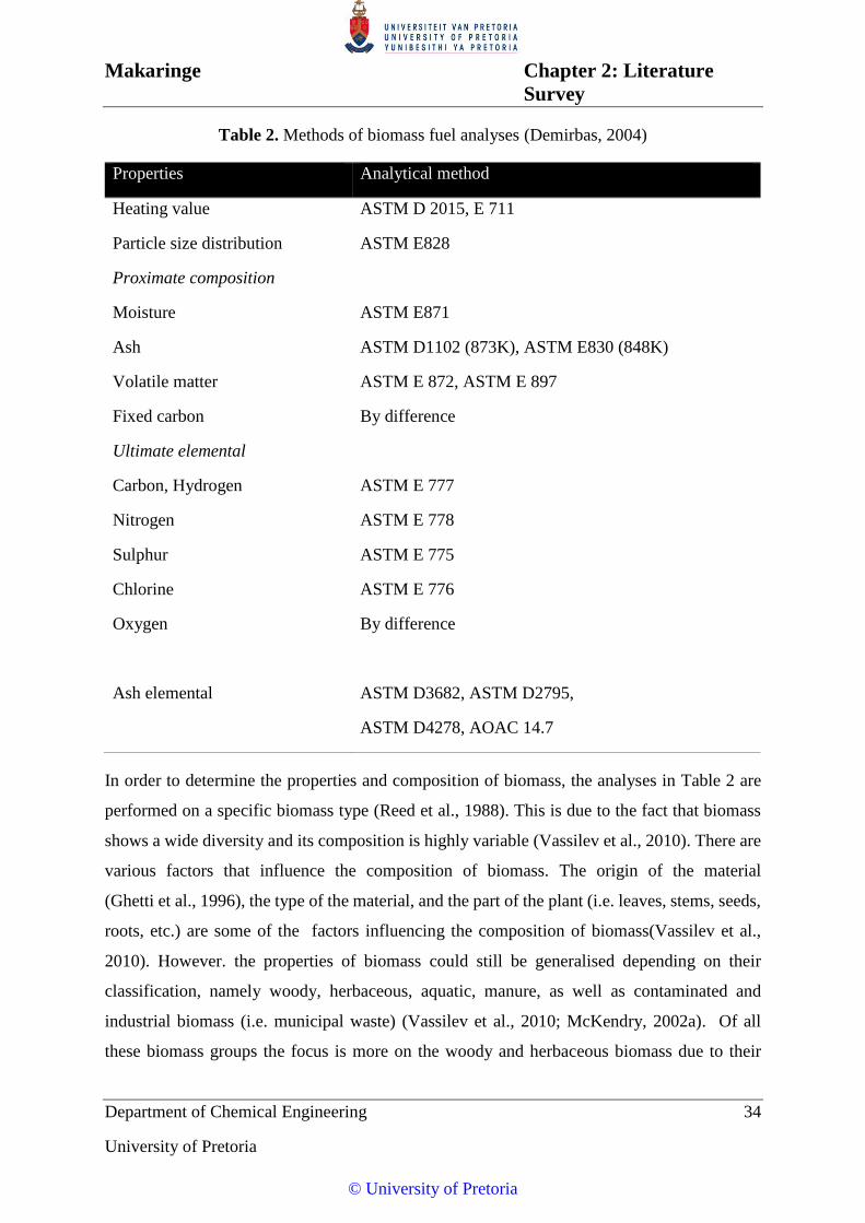
Table 2. Methods of biomass fuel analyses (Demirbas, 2004)
Properties Analytical method
Heating value
Particle size distribution
Proximate composition
Moisture
Ash
Volatile matter
Fixed carbon
Ultimate elemental
Carbon, Hydrogen
Nitrogen
Sulphur
Chlorine
Oxygen
Ash elemental
ASTM D 2015, E 711
ASTM E828
ASTM E871
ASTM D1102 (873K), ASTM E830 (848K)
ASTM E 872, ASTM E 897
By difference
ASTM E 777
ASTM E 778
ASTM E 775
ASTM E 776
By difference
ASTM D3682, ASTM D2795,
ASTM D4278, AOAC 14.7
In order to determine the properties and composition of biomass, the analyses in Table 2 are
performed on a specific biomass type (Reed et al., 1988). This is due to the fact that biomass
shows a wide diversity and its composition is highly variable (Vassilev et al., 2010). There are
various factors that influence the composition of biomass. The origin of the material
(Ghetti et al., 1996), the type of the material, and the part of the plant (i.e. leaves, stems, seeds,
roots, etc.) are some of the factors influencing the composition of biomass(Vassilev et al.,
2010). However. the properties of biomass could still be generalised depending on their
classification, namely woody, herbaceous, aquatic, manure, as well as contaminated and
industrial biomass (i.e. municipal waste) (Vassilev et al., 2010; McKendry, 2002a). Of all
these biomass groups the focus is more on the woody and herbaceous biomass due to their
© University of Pretoria
Makaringe Chapter 2: Literature
Survey
Department of Chemical Engineering 35
University of Pretoria
lower moisture content (McKendry, 2002a). The general properties of these two groups of
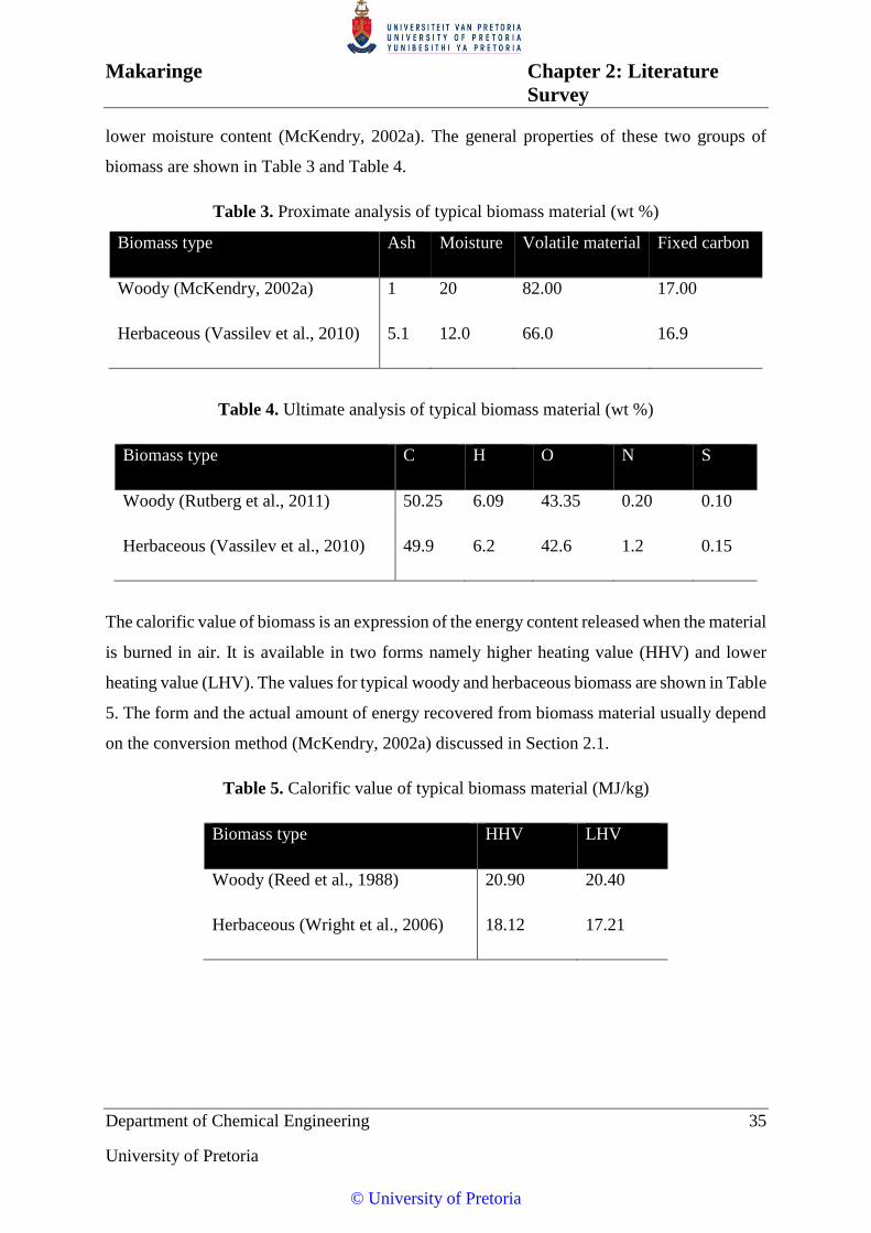
biomass are shown in Table 3 and Table 4.
Table 3. Proximate analysis of typical biomass material (wt %)
Biomass type Ash Moisture Volatile material Fixed carbon
Woody (McKendry, 2002a) 1 20 82.00 17.00
Herbaceous (Vassilev et al., 2010) 5.1 12.0 66.0 16.9
Table 4. Ultimate analysis of typical biomass material (wt %)
Biomass type C H O N S
Woody (Rutberg et al., 2011) 50.25 6.09 43.35 0.20 0.10
Herbaceous (Vassilev et al., 2010) 49.9 6.2 42.6 1.2 0.15
The calorific value of biomass is an expression of the energy content released when the material
is burned in air. It is available in two forms namely higher heating value (HHV) and lower
heating value (LHV). The values for typical woody and herbaceous biomass are shown in Table
5. The form and the actual amount of energy recovered from biomass material usually depend
on the conversion method (McKendry, 2002a) discussed in Section 2.1.
Table 5. Calorific value of typical biomass material (MJ/kg)
Biomass type HHV LHV
Woody (Reed et al., 1988) 20.90 20.40
Herbaceous (Wright et al., 2006) 18.12 17.21
© University of Pretoria

Makaringe Chapter 2: Literature
Survey
Department of Chemical Engineering 36
University of Pretoria
2.4.5 COMPOSITION OF SELECTED BIOMASS TYPES USED IN THIS STUDY FOUND IN
LITERATURE
The proximate and ultimate analysis of Napier grass, peach pips, bamboo and pine tree are
shown in Table 6 and Table 7.
Table 6. Proximate analysis of selected biomass material
Biomass type (and references) Ash
(%)
Moisture
(%)
Volatile
material
(%)
Fixed
carbon
(%)
LHV
(MJ/kg)
Nappier grass (TC et al., 2002; Lee et al.,
2010)
9.68 9.43 72.58 8.38 18.00
Peach pips (Parikh et al., 2005) 1.10 - 79.10 19.80 19.42
Bamboo (Channiwala and Parikh, 2002) 1.95 11.50 86.80 11.24 20.55
Pine tree (Cuiping et al., 2004) 0.89 8.61 76.50 14.45 19.38
Table 7.Ultimate analysis of biomass material used in this study
Biomass type (and references) C H O N S Cl
Nappier grass (Lee et al., 2010) 42.40 5.98 45.32 1.71 0.09 0.24
Peach pips (Parikh et al., 2005) 49.14 6.34 43.52 0.48 0.02 -
Bamboo (Channiwala and
Parikh, 2002)
55.8 4.8 38.1 1.3 - -
Pine tree (Cuiping et al., 2004) 49.41 7.67 42.19 0.1 0.05 -
2.4.6 BIOMASS THERMAL CHARACTERISATION
The thermal behaviour of biomass is an important characteristic. Thermal analysis is a
technique in which the mass and/or energy content of a solid material is measured as a function
of temperature whilst the material is subjected to a controlled temperature programme (Inczedy
© University of Pretoria

Makaringe Chapter 2: Literature
Survey
Department of Chemical Engineering 37
University of Pretoria
et al., 1998). There are several techniques used to conduct thermal analysis of solid material.
These techniques (i.e. thermogravinetric analysis (TGA), differential thermal analysis (DTA),
differential scanning calorimetric (DSC), etc.) are usually applied when characterising biomass
(Yang et al., 2007; Stenseng et al., 2001).
2.4.6.1 THERMOGRAVIMETRIC ANALYSIS
Thermogravimetric analysis (TGA) is a method of thermal analysis in which a mass loss of a
material is measured as a function of increasing temperature (with constant heating rate) or as
a function of time. Thermal properties of biomass have been investigated using TGA analysis.
The results obtained during TGA play a significant role when computing the kinetics of
biomass (Bassilakis et al., 2001; Mansaray and Ghaly, 1999; Kumar et al., 2008; Slopiecka et
al., 2012; Wongsiriamnuay and Tippayawong, 2010; Hui et al., 2010).
Characteristics of biomass differs per type. Pyrolysis of biomass takes place in different stages
illustrated in Figure 16. The moisture content is removed first from the material at ~100 °C.
This is followed by the removal of volatile materials in a second stage at temperatures between
250 - 450 °C. From Figure 16 it can be seen that a fraction of char and ash is left at the end. If
the process is carried in the presence of air char will burn leaving the ash as the final residue
(Reed et al., 1988).
The three stages of biomass pyrolysis happen due to the presence of three major components
of biomass discussed in section 2.4.2. The weight percentage of these components in a specific
biomass influence its thermal behaviour. When taking into consideration the water evolution
stage, the biomass pyrolysis could sometimes be said to happen in four stages namely: the
dehydration, hemicellulose decomposition, cellulose decomposition and finally the lignin
decomposition (Yang et al., 2007). However, in most cases the hemicellulose and cellulose are
said to decompose during active pyrolysis (Gašparovič et al., 2010) hence the pyrolysis of
biomass is sometimes said to be divided into three stages.
© University of Pretoria

Makaringe Chapter 2: Literature
Survey
Department of Chemical Engineering 38
University of Pretoria
Figure 16. TGA curve of a general biomass sample in the absence of air
(Reed et al., 1988)
Each type of biomass produces slightly different quantities of char, volatiles and ash.
Knowledge of these quantities, as well as the temperature dependencies of the reaction and
associated weight losses, are useful in understanding gasifier operation and design
(Reed et al., 1988)
© University of Pretoria

Department of Chemical Engineering 39
University of Pretoria
3 DESCRIPTION OF EXPERIMENTAL EQUIPMENT
3.1 TGA-FTIR INSTRUMENT
The Perkin-Elmer TGA-FTIR hyphenated system (TGA 4000 and Spectrum 100) (Figure 17)
was used for the characterisation of the biomass samples. This instrument can reach a
maximum temperature of 1000 o C and a maximum heating rate of 200 o C/min. The instrument
uses an alumina pan as a sample holder. The sample size that can fit in to the pan depend on
the sample density. It is advisable to have the samples in a powder form. The samples were
placed into a pan using a spatula to avoid contamination with moisture from human skin. A
pair of tweezers was used to carefully hold the pan and place it into the TGA furnace. Prior to
biomass characterisation the TGA was calibrated using a metal ball with a mass of 56 mg.
Calcium hydroxide powder was then used as a reference sample.
Figure 17. PerkinElmer TGA-FTIR instrument
© University of Pretoria

Makaringe Chapter 3: Description of
Experimental Equipment
Department of Chemical Engineering 40
University of Pretoria
3.2 PLASMA GASIFICATION SYSTEM
The plasma gasification system which was used for the biomass gasification experiments is
shown in Figure 18. The system consist of four main components which are the plasma reactor
(consisting of the plasma torch, quench probe, feeding pipe and the glass view part), knockout
vessel, filter trap and the sampling point. The main utilities of the system is the cooling water
from the cooling towers which are placed outside the laboratory under covered roof with open
sides, plasma power supply and a ventilation system connected to the building’s ventilation
system.
Plasma
Reactor
Quench
Probe
Hopper
Screw feeder
Argon
cylinder
Oxygen
cylinder
Nitrogen
cylinder
Water trap
Ventilation
U-Tube
for sampling
FilterPlasma
torch
Figure 18. Laboratory scale plasma gasification system
3.2.1 PLASMA REACTOR
The plasma reactor is the heart of the gasification system (Figure 19). It consists of a stainless
steel chamber, the ceramic crucible fitted inside the reactor chamber (the crucible is fitted to
prevent heat loss to the walls of the reactor). Between the stainless steel chamber and the
ceramic crucible there is a fine sand to further reduce heat loss. The outside walls of the reactor
and the bottom flange are water cooled. The ceramic lid is placed on top of the ceramic crucible
before covering the reactor with a stainless steel lid to ensure that more the heat supplied into
the reactor is contained inside the ceramic crucible. The lid of the reactor contains four holes.
© University of Pretoria

Makaringe Chapter 3: Description of
Experimental Equipment
Department of Chemical Engineering 41
University of Pretoria
Figure 19. Plasma gasification reactor
One hole is for fitting the plasma torch (Figure 20) which is the main component of the plasma
reactor. The plasma torch consist of the anode and the cathode which are mainly made of
tungsten or copper. The torch is operated by means of a 30 kW plasma power supply (Figure
21). The power supplied into the system can be changed by adjusting the current settings
depending on the required operating temperature. In this study the power varied between 13-
16 kW.
Figure 20. Plasma torch
© University of Pretoria

Makaringe Chapter 3: Description of
Experimental Equipment
Department of Chemical Engineering 42
University of Pretoria
Figure 21. A 30 KW plasma power supply
The second hole on the reactor lid is fitted with a quench probe (Figure 22). The specialised
heat exchanger has a 68 mm outer pipe fitted with a 42.5 mm inner probe. Both the outer and
the inner probe are water cooled. The product gases of the gasification process exit through the
quench probe. The gas is cooled to ~ 40 °C before it enters the knockout vessel.
Figure 22. Quench probe
© University of Pretoria

Makaringe Chapter 3: Description of
Experimental Equipment
Department of Chemical Engineering 43
University of Pretoria
The third hole of the reactor lid is fitted with a feeder pipe attached to the feeding hopper
(Figure 23). The pipe is 100 mm in diameter and it is also cooled with water. This is done
shield thermal radiation from the feeder pipe to prevent pre-gasification.
Figure 23. Feeding hopper
The fourth holes is a view part sealed with a transparent quartz glass. This glass is used to view
the inside of the reactor during operation. Also this glass is used for monitoring the temperature
of the reactor by using an optical pyrometer in case the type R thermocouple breaks.
There lid also has a nozzle which is used for introducing the reagent directly into the reactor.
The other option is to introduce the reagent through the plasma torch.
3.2.2 KNOCKOUT VESSEL
Water is one of the products of the gasification process. Any water vapour available in the
product gas will condense after being cooled trough a quench probe. The knock out vessel
(Figure 24) is use to separate water and any available particulates from the syngas. The gas
flow straight into the top of the vessel through a 40 mm pipe. The water and the particulates
precipitates at the bottom of the vessel while the syngas flow through a pipe at the side of the
vessel into a filter trap. The vessel has a 200 mm OD, and with a 50 mm throat.
© University of Pretoria

Makaringe Chapter 3: Description of
Experimental Equipment
Department of Chemical Engineering 44
University of Pretoria
Figure 24. Knockout vessel
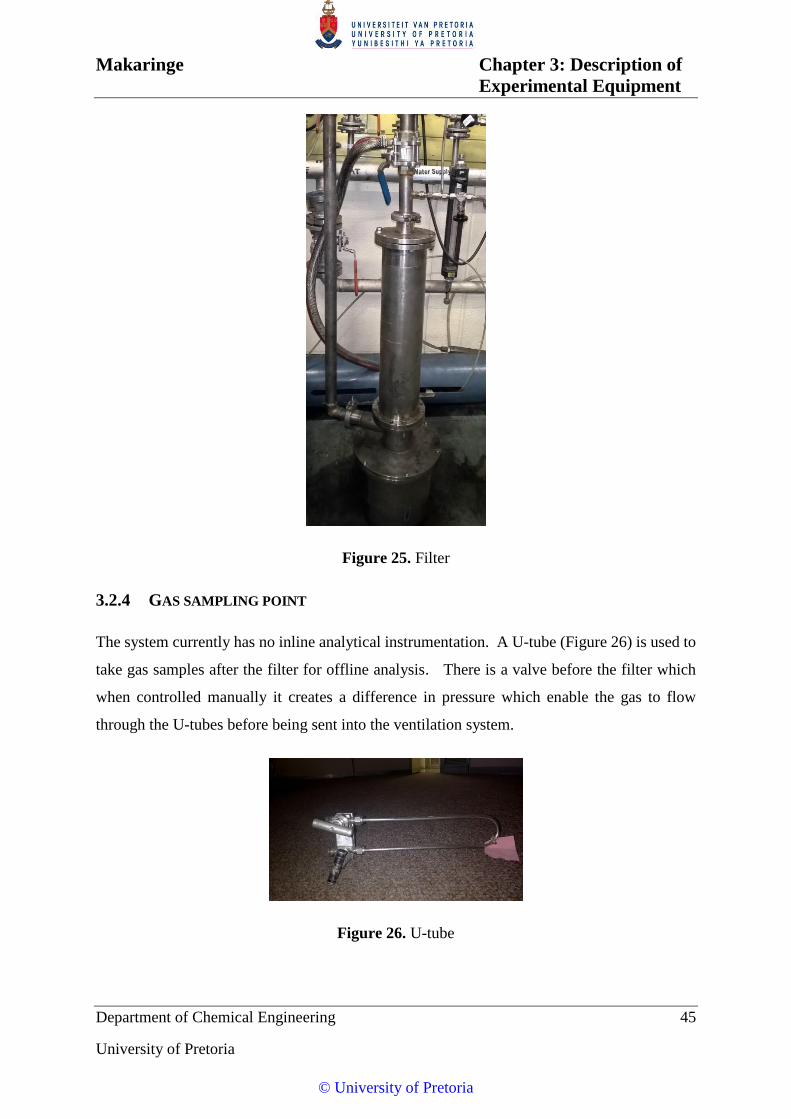
3.2.3 FILTER
After the knockout vessel the syngas flows through a filter trap (Figure 25). The filter is fitted
with a filter bag used to filter the fine solid ash present in the gas. It also has a pot below the
bag where any particulates that weren’t trapped by the knockout pot can accumulate.
© University of Pretoria
Makaringe Chapter 3: Description of
Experimental Equipment
Department of Chemical Engineering 45
University of Pretoria
Figure 25. Filter
3.2.4 GAS SAMPLING POINT
The system currently has no inline analytical instrumentation. A U-tube (Figure 26) is used to
take gas samples after the filter for offline analysis. There is a valve before the filter which
when controlled manually it creates a difference in pressure which enable the gas to flow
through the U-tubes before being sent into the ventilation system.
Figure 26. U-tube
© University of Pretoria

Department of Chemical Engineering 46
University of Pretoria
4 TGA EXPERIMENTS
TGA experiments were conducted at the laboratories of the Fluoro-materials Group at the
University of Pretoria. This study was carried out to investigate the decomposition mechanisms
and reaction kinetics of different biomass materials.
4.1 MATERIALS
Biomass samples used in this work were Napier grass (Pennisetum pupureum), peach pips
(Prunus persica (L.) Batsch), bamboo wood (Bambusa balcooa) and pine wood (Pinus patula).
All samples were sourced from local suppliers of forestry products, except the bamboo, which
was taken from the University of Pretoria’s botanical garden. Nitrogen gas (>99.999%) was
obtained from African Oxygen Ltd, and used as received
4.2 SAMPLE PREPARATION
The biomass samples were prepared by first cutting the material into small pieces and then by
milling using a Retsch mill (Type SR 200, Model 70546). The samples were further sieved in
order to obtain a fine fraction.
4.3 THERMOGRAVIMETRIC ANALYSIS
The TGA-FTIR analysis was performed using a Perkin Elmer TGA 4000 coupled to a Perkin
Elmer Spectrum 100 FTIR spectrometer. The gases evolved from the TGA were transferred to
a heated infrared cell (kept at 250 °C) via a heated stainless steel transfer line (kept at 250 °C).
The IR cell was fitted with KBr single crystal windows and had a beam path length of 10 cm.
For each TGA experiment, approximately 20 mg of sample was placed in an alumina crucible.
Thermograms were recorded from ~25 °C to 950 °C at three different heating rates, viz.: 20,
100 and 200 oC/min under nitrogen atmosphere flowing at a rate of 20 ml/min, then kept
isothermal for 15 minutes. The end temperature is close to the operating temperature of
gasification system. The FTIR spectrometer was set to scan from 4000 cm-1 to 550 cm-1 at a
rate of one spectrum every 6 seconds with frequency resolution of 1 cm-1.
© University of Pretoria

Makaringe Chapter 4: TGA Experiments
Department of Chemical Engineering 47
University of Pretoria
4.4 RESULTS AND DISCUSSION
4.4.1 PYROLYSIS UNDER NITROGEN
The TGA-FTIR results for the different biomass which were tested under a nitrogen
atmosphere are discussed below.
4.4.1.1 BAMBOO MATERIAL
The TGA along with the corresponding differential thermogravimetric (DTG) curves for
bamboo at heating rates of 20, 100 and 200 °C/min are shown in Figure 27 and Figure 28.
Figure 27. TGA curves of bamboo at 20, 100 and 200 °C/min under nitrogen.
© University of Pretoria
Makaringe Chapter 4: TGA Experiments
Department of Chemical Engineering 48
University of Pretoria
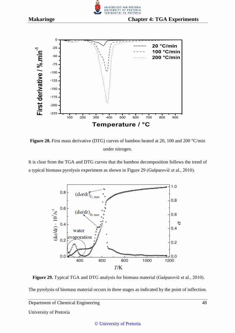
Figure 28. First mass derivative (DTG) curves of bamboo heated at 20, 100 and 200 °C/min
under nitrogen.
It is clear from the TGA and DTG curves that the bamboo decomposition follows the trend of
a typical biomass pyrolysis experiment as shown in Figure 29 (Gašparovič et al., 2010).
Figure 29. Typical TGA and DTG analysis for biomass material (Gašparovič et al., 2010).
The pyrolysis of biomass material occurs in three stages as indicated by the point of inflection.
© University of Pretoria

Makaringe Chapter 4: TGA Experiments
Department of Chemical Engineering 49
University of Pretoria
This is due to the decomposition of its three main components, viz. hemicellulose, cellulose
and lignin (Yang et al., 2007). The first stage is predominantly dehydration, occurring at
temperatures below ~200 °C for bamboo (Figure 27 and Figure 28). The dehydration
temperatures differ for each heating rate. The maximum dehydration temperatures was 81 °C
for a heating rate of 20 °C/min, 110.7 °C for the 100 °C/min and 123.4 °C for 200 °C/min
(Figure 28). The maximum dehydration rates were 1.417, 4.918 and 8.828 wt %/min for the
20, 100 and 200 °C/min respectively.
The second stage comprises active pyrolysis. The decomposition of hemicellulose and
cellulose stages are grouped together in this stage. The hemicellulose decomposition takes
place first (mainly in the temperature range 220-315 °C) followed by the decomposition of the
cellulose between 314-400 °C (Yang et al., 2007; Gašparovič et al., 2010; Mui et al., 2008).
The hemicellulose decomposition of the bamboo material is indicated by the slight shoulder in
the DTG curve in Figure 28 (which is similar to that in Figure 29). This shoulder is clearly
visible for the heating rates of 20 and 100 °C/min. The decomposition temperatures obtained
in this case fall within temperature ranges mentioned in the literature; but it was noticed that
as the heating rate was increased so did the temperature range of decomposition.
The shoulder in the DTG curves for bamboo ranged fell in the range 250-312 °C for the heating
rate of 20°C/min and 280-348 °C for the heating rate of 100°C/min. This shoulder which is
associated with hemicellulose decomposition was not visible at the heating rate of 200 °C/min.
Instead a sharp smooth peak was obtained at temperatures between 290 and 440 °C. This sharp
curve is associated with the decomposition of the cellulose and it can be said to be the
maximum decomposition rate for the whole material. The maximum decomposition
temperatures (maximum peak associated with cellulose decomposition) for the 20 and 100
°C/min were 353.7 °C and 380.67 °C respectively. The maximum decomposition rates obtained
were 17.9, 97.4 and 192 %/min for the heating rates of 20, 100 and 200 °C/min respectively.
The third stage is termed passive pyrolysis. Lignin (which is more thermally stable)
decomposes here, in a wide range temperatures from 160 to 900 °C (Yang et al., 2007). Based
on the temperature range at which lignin is said to decompose, it is clear that it decomposes in
both active and passive pyrolysis regions but without noticeable peaks (Slopiecka et al., 2012).
It is during this stage that the final weight conversion happened at a rate between 1.84 and 1.57
© University of Pretoria

Makaringe Chapter 4: TGA Experiments
Department of Chemical Engineering 50
University of Pretoria
%/min for the heating rate of 20 °C/min, 7.9 and 0.166 %/min for the 100 °C/min and 19.9 and
0.400 %/min for the 200 °C/min.
4.4.1.1.1 EFFECT OF HEATING RATE
The heating rate is known to have an effect on the process. This is observed in Figure 27 &
Figure 28. As the heating rate increases the curve shifts towards high temperatures. Hence the
dehydration temperature obtained at a heating rate of 200 °C/min was higher than that at 20
and 100 °C/min. The heating rate also affects the start and the end temperatures of each stage
(i.e. dehydration, active and passive pyrolysis stages). In short it can be concluded that as the
heating rate was increased, firstly the TGA curve shifted towards high temperatures, secondly
the maximum decomposition rate increased and finally the conversion increased (though the
deference in conversion was slight for the heating rate of 100 and 200 °C/min). The shift of
the curves towards high temperature is explained on the basis of heat transfer limitation. For
low heating rates, more time is available for the sample to reach thermal equilibrium. It should
also be noted that the temperature is measured below the sample holder, not in the sample.
Thus a small difference between the recorded and the actual temperature is expected. The
difference is greater for faster heating rates. In addition chemical kinetic effects are more
pronounced at slower heating rates. These effects cause the curves to shift to the right
(Slopiecka et al., 2012). The effect of the heating rate on gases released is discussed on the next
section.
The char residues which remained were found to be 21.5, 19.6 and 19.4 % for the 20, 100 and
200 °C/min (Figure 28). Thus it can be concluded that higher pyrolysis rates lead to more
effective gasification.
4.4.1.1.2 FTIR RESULTS
An inline FTIR instrument was used to analyse the gases released during pyrolysis. Ideally the
main product of the gasification process should be hydrogen (H2) and carbon monoxide (CO)
with some carbon dioxide and hydrocarbons like methane. The TGA characterisation
experiments does not correspond exactly with what is happening inside a gasifiers. It merely
gives an indication as to what to expect. Therefore gases released during TGA experiments are
not exactly what will be released during our plasma gasification.
© University of Pretoria

Makaringe Chapter 4: TGA Experiments
Department of Chemical Engineering 51
University of Pretoria
Figure 30, Figure 31 and Figure 32 shows the FTIR spectra (4 spectra per heating rate) for
bamboo. The first graph for each heating rate (82 °C for 20 °C/min, 107 °C for 100 °C/min and
117 °C for 200 °C/min) correspond to the dehydration stage. It can be seen from each spectrum
that mostly water peaks appear here. There are noticeable water peaks at wave numbers of
~3600 and 1500 cm-1. These peaks validate what was observed from the TGA results discussion
(water evaporation during the first stage of the decomposition process as seen in the DTG
curves Figure 28). The effect of heating rate is observed here as well. The higher the heating
rate, the higher the observed dehydration temperatures and the higher the absorption units of
the peaks including that of carbon dioxide which was observed at this stage at a wave number
of 2380 cm-1. It is considerably smaller than the other CO2 peaks obtained during active
pyrolysis (especially during higher heating rates). During active pyrolysis, the CO2 peak is
immediately noticed (second and third spectrum from different heating rates). A second CO2
peak is observed at a wavenumber of 670 cm-1. The other noticeable peak at 1800 cm-1 belong
to aldehydes. Though it is relatively small compared to other peaks, the carbon monoxide peak
(which is the peak of interest) is observed during active pyrolysis at wave number 2150 cm-1.
© University of Pretoria

Makaringe Chapter 4: TGA Experiments
Department of Chemical Engineering 52
University of Pretoria
Figure 30. FTIR spectra of bamboo heated at 20 °C/min under nitrogen.
© University of Pretoria
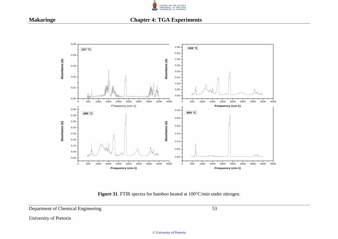
Makaringe Chapter 4: TGA Experiments
Department of Chemical Engineering 53
University of Pretoria
0 500 1000 1500 2000 2500 3000 3500 4000 4500
0.00
0.01
0.02
0.03
0.04
0.05
0 500 1000 1500 2000 2500 3000 3500 4000 4500
0.00
0.05
0.10
0.15
0.20
0.25
0.30
0.35
0.40
0 500 1000 1500 2000 2500 3000 3500 4000 4500
0.00
0.05
0.10
0.15
0.20
0.25
0.30
0.35
0.40
0 500 1000 1500 2000 2500 3000 3500 4000 4500
0.00
0.05
0.10
0.15
0.20
0.25
0.30
Ab
sorb
ance
(A
)
Frequency (cm-1)
107 °C
Ab
sorb
ance
(A
)
Frequency (cm-1)
349 °C
Ab
sorb
ance
(A
)
Frequency (cm-1)
380 °C
Ab
sorb
ance
(A
)Frequency (cm-1)
950 °C
Figure 31. FTIR spectra for bamboo heated at 100°C/min under nitrogen.
© University of Pretoria

Makaringe Chapter 4: TGA Experiments
Department of Chemical Engineering 54
University of Pretoria
0 500 1000 1500 2000 2500 3000 3500 4000 4500
0.00
0.01
0.02
0.03
0.04
0.05
0 500 1000 1500 2000 2500 3000 3500 4000 4500
0.0
0.1
0.2
0.3
0.4
0.5
0.6
0 500 1000 1500 2000 2500 3000 3500 4000 4500
0.0
0.1
0.2
0.3
0.4
0 500 1000 1500 2000 2500 3000 3500 4000 4500
0.0
0.1
0.2
0.3
0.4
Ab
sorb
ance
(A
)
Frequency (cm-1)
117 °C
Ab
sorb
ance
(A
)
Frequency (cm-1)
284 °C
Ab
sorb
ance
(A
)
Frequency (cm-1)
352 °C
Ab
sorb
ance
(A
)
Frequency (cm-1)
950 °C
Figure 32. FTIR spectra of bamboo heated at 200°C/min under nitrogen.
© University of Pretoria

Makaringe Chapter 4: TGA Experiments
Department of Chemical Engineering 55
University of Pretoria
A methane peak was clearly observed at 3000 cm-1 while other group of alkanes were observed
at 1200 cm-1. Methane and other hydrocarbons are known to be the main product of fast
pyrolysis operated at temperatures up to 500 °C with short residence time (~1 sec). Therefore
their presence during the TGA decomposition of biomass material is expected.
As mentioned earlier, the heating rate also affects the peak quantities of the gases released. The
high the heating rate, the higher the peaks. For examples, the CO2 peak has an absorption unit
of up to 0.09 for the 20 °C/min, 0.4 for the 100 °C/min and up to 0.6 for the 200 °C/min. This
is expected as at slower heating rates there is more time for the evolving gases to pass through
the gas line and lower concentrations will be observed.
4.4.1.2 COMPARISON BETWEEN FOUR MATERIALS
The TGA-FTIR results for pine tree, peach pips and Napier grass are shown in the Appendix
A. The behaviour of these materials during pyrolysis is similar to that of bamboo discussed
above, but with noticeable difference.
The maximum decomposition rates obtained during active pyrolysis for the heating rate of
20 °C/min is 12.5, 17.9, 18.9 and 19.6 wt %/min for peach pips, bamboo, Napier grass and pine
wood respectively. The pine tree showed to have high decomposition rate as compared to the
other three materials. The same trend happened under 100 °C/min. Pine tree had the highest
decomposition rate of 99.5 wt %/min while peach pips had the lowest decomposition rate of
66.85 wt %/min. However when the heating rate was increased to 200 °C/min Napier grass
seemed to decompose at the fastest rate of 266.8 wt %/min as observed in Figure 34.
© University of Pretoria

Makaringe Chapter 4: TGA Experiments
Department of Chemical Engineering 56
University of Pretoria
0 100 200 300 400 500 600 700 800 900
0
10
20
30
40
50
60
70
80
90
100
Ma
ss
pe
rce
nta
ge
(%
)
Temperature (°C)
Napier grass
Bamboo
Peach pips
Pine wood
Figure 33. TGA of Napier grass, pine wood, bamboo and peach pips heated at 200 °C/min
under nitrogen.
0 100 200 300 400 500 600 700 800 900
-300
-275
-250
-225
-200
-175
-150
-125
-100
-75
-50
-25
0
Fir
st
de
riv
ati
ve
(%
/min
)
Temperature (°C)
Bamboo
Napier grass
Pine wood
Peach pips
Figure 34. DTG of Napier grass, pine wood, bamboo and peach pips heated at 200 °C/min
under nitrogen.
© University of Pretoria

Makaringe Chapter 4: TGA Experiments
Department of Chemical Engineering 57
University of Pretoria
Although Napier grass decomposed at a fastest rate, it had low conversion (Figure 33). The
residues remaining at the end of the process were 12.4, 19.5, 21.2 and 26.6 weight percentage
for pine, bamboo, peach pips and Napier grass respectively. These conversion correspond to
those in the literature for most biomass materials under nitrogen atmospheres (Kumar et al.,
2008).
The same heating rate effect that was observed on bamboo was also observed on the other three
materials. At high heating rates higher conversion was achieved and the materials decomposes
at a faster rate. However it should be noted that some materials decompose faster than the
others as discussed above.
The FTIR spectra (shown in the Appendix A) for the other three materials show similarities to
FTIR spectra of bamboo. At low temperatures (the first stage of pyrolysis) the volume of
volatiles released were low. As the temperature is increased, the peaks height start to increase,
resulting in clearer and sharper peaks. Even though the peak heights at low temperatures are
small, the water peaks can still be identified in all materials. As discussed previously, this stage
is due to dehydration, hence water peaks are expected. The peak identifications are discussed
in detail under the discussion of bamboo material in Section 4.5.
4.4.2 OXYGEN ATMOSPHERES
4.4.2.1 TGA AND DTG RESULTS OBTAINED UNDER OXYGEN
As mentioned earlier, results obtained from TGA characterisation were used as a guideline as
to what to expect when gasifying the biomass in a plasma system. The same four material
studied previously were also characterised in a TGA-FTIR instrument under oxygen. The
conditions were kept the same as under nitrogen atmospheres. The analyses were also done at
three different heating rates namely 20, 100 and 200 °C. The resulting TGA and DTG curves
are shown in the Appendix C, D, and E.
Figure 35 and Figure 36 compare the TGA and DTG results for pine, bamboo, Napier grass
and peach pips at a heating rate of 200 °C/min under oxygen atmospheres.
© University of Pretoria

Makaringe Chapter 4: TGA Experiments
Department of Chemical Engineering 58
University of Pretoria
0 100 200 300 400 500 600 700 800 900
0
10
20
30
40
50
60
70
80
90
100
Ma
ss
pe
rce
nta
ge
(%
)
Temperature (°C)
Napier grass
Peach pips
Pine wood
Bamboo
Figure 35. TGA of Napier grass, pine wood, bamboo and peach pips at a heating rate of
200 °C/min under oxygen.
0 100 200 300 400 500 600 700 800 900
-250
-200
-150
-100
-50
0
Fir
st
de
riv
ati
ve
(%
/min
)
Temperature (°C)
Napier grass
Peach pips
Pine wood
Bamboo
Figure 36. DTG of Napier grass, pine wood, bamboo and peach pips at a heating rate of
200 °C/min under oxygen.
© University of Pretoria

Makaringe Chapter 4: TGA Experiments
Department of Chemical Engineering 59
University of Pretoria
It is observed from Figure 35 that the conversion achieved under oxygen is high compared to
that under nitrogen; obviously since combustion now takes place. For all materials conversion
was above 90 %. Napier grass was still found to have low conversion (~92.8%) compared to
the other three materials. Pine tree was found to have the highest conversion (~99 %) followed
by peach pips (~98.8 %) and bamboo (~98 %). Napier grass was still decomposing at a highest
rate when compared to other materials (Figure 36).
The effect of the heating rate observed under oxygen is the same as under nitrogen. The TGA
curves shifted towards high temperatures as the heating rate was increased. However, the effect
of heating rate on conversion was not significant. If one wanted to make a distinction it could
still be noticed that the residues remaining after pyrolysis were a little bit less for the heating
rate of 200 °C/min compared to other heating rates (i.e 20 & 100 °C/min). The decomposition
rate also increased as the heating rate increased. The decomposition rate achieved at a heating
rate of 200 °C/min were 214. 7 %/min for Napier grass, 187.5 %/min for pine, 186.8 %/min
for bamboo and 149.9 %/min for peach pips.
4.4.2.2 FTIR RESULTS OBTAINED UNDER OXYGEN ATMOSPHERES
In Chapter two pyrolysis was defined as a thermal decomposition occurring in the absence of
oxygen. Once the organic material decomposes in the presence of oxygen the process is called
combustion and the product of combustion is water and carbon dioxide according to this
reaction of a typical biomass sample (Equation 6).
)(72.003.1 22266.044.1 heatCOOHOOCH 6
Once the biomass is partially combusted the process is called gasification and the resulting
products are mainly a mixture of carbon monoxide and hydrogen, referred to as syngas. When
the TGA analysis is conducted under oxygen, the amount of oxygen is not controlled according
to the gasification stoichiometry. The FTIR results (Figure 37 to Figure 40) shows that the
resulting products during TGA experiment under oxygen is mostly carbon dioxide at wave
number ~2380 and ~670 cm-1) and water (at wave number ~3600 and ~500 cm-1). This is
observed especially as the operating temperature increases. However peach pips material
behaved differently for identical gas flow rates. Other pyrolysis gases (discussed in Section
4.4.1) are more visible in the FTIR results for peach pips (Figure 40).
© University of Pretoria

Makaringe Chapter 4: TGA Experiments
Department of Chemical Engineering 60
University of Pretoria
0 500 1000 1500 2000 2500 3000 3500 4000 4500
-0.03
-0.02
-0.01
0.00
0.01
0.02
0.03
0 500 1000 1500 2000 2500 3000 3500 4000 4500
0.0
0.1
0.2
0.3
0.4
0.5
0.6
0.7
0.8
0.9
1.0
1.1
1.2
1.3
0 500 1000 1500 2000 2500 3000 3500 4000 4500
0.0
0.1
0.2
0.3
0.4
0.5
0.6
0.7
0.8
0.9
1.0
Ab
so
rban
ce (
A)
Frequency (cm-1)
123 °C
Ab
so
rban
c (
A)
Frequency (cm-1)
351 °C
Ab
so
rban
c (
A)
Frequency (cm-1)
900 °C
Figure 37. FTIR spectra of bamboo at a heating rate of 200 °C/min under oxygen.
© University of Pretoria

Makaringe Chapter 4: TGA Experiments
Department of Chemical Engineering 61
University of Pretoria
0 500 1000 1500 2000 2500 3000 3500 4000 4500
-0.03
-0.02
-0.01
0.00
0.01
0.02
0.03
0 500 1000 1500 2000 2500 3000 3500 4000 4500
0.0
0.1
0.2
0.3
0.4
0.5
0.6
0.7
0.8
0.9
1.0
1.1
1.2
1.3
0 500 1000 1500 2000 2500 3000 3500 4000 4500
0.0
0.1
0.2
0.3
0.4
0.5
0.6
0.7
0.8
0.9
1.0
Ab
so
rban
ce (
A)
Frequency (cm-1)
123 °C
Ab
so
rban
c (
A)
Frequency (cm-1)
351 °C
Ab
so
rban
c (
A)
Frequency (cm-1)
900 °C
Figure 38. FTIR of pine wood at 200°C/min under oxygen.
© University of Pretoria

Makaringe Chapter 4: TGA Experiments
Department of Chemical Engineering 62
University of Pretoria
0 500 1000 1500 2000 2500 3000 3500 4000 4500
-0.025
-0.020
-0.015
-0.010
-0.005
0.000
0.005
0.010
0.015
0.020
0.025
0 500 1000 1500 2000 2500 3000 3500 4000 4500
0.0
0.2
0.4
0.6
0.8
1.0
1.2
0 500 1000 1500 2000 2500 3000 3500 4000 4500
-0.1
0.0
0.1
0.2
0.3
0.4
0.5
0.6
0.7
0.8
0.9
1.0
Ab
so
rban
ce (
A)
Frequency (cm-1)
123 °C
Ab
so
rban
c (
A)
Frequency (cm-1)
319 °C
Ab
so
rban
c (
A)
Frequency (cm-1)
840 °C
Figure 39. FTIR spectra of Napier grass at a heating rate of 200°C/min under oxygen.
© University of Pretoria
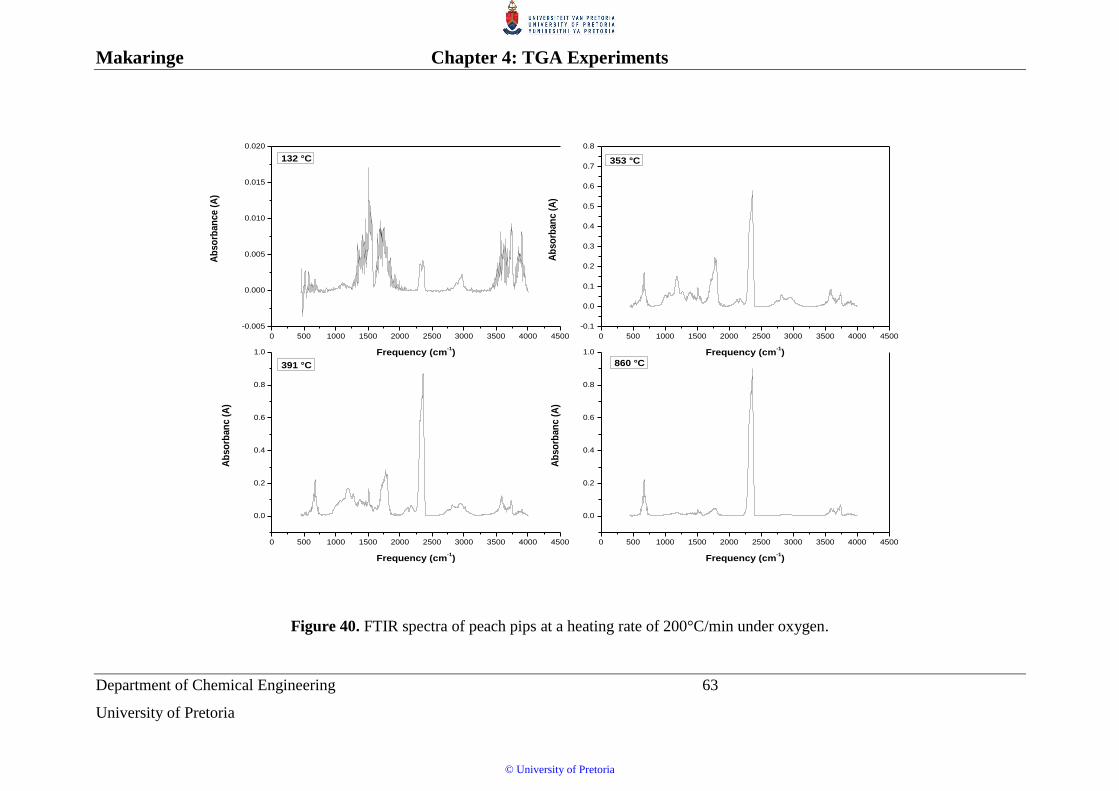
Makaringe Chapter 4: TGA Experiments
Department of Chemical Engineering 63
University of Pretoria
0 500 1000 1500 2000 2500 3000 3500 4000 4500
-0.005
0.000
0.005
0.010
0.015
0.020
0 500 1000 1500 2000 2500 3000 3500 4000 4500
-0.1
0.0
0.1
0.2
0.3
0.4
0.5
0.6
0.7
0.8
0 500 1000 1500 2000 2500 3000 3500 4000 4500
0.0
0.2
0.4
0.6
0.8
1.0
0 500 1000 1500 2000 2500 3000 3500 4000 4500
0.0
0.2
0.4
0.6
0.8
1.0
Ab
so
rban
ce (
A)
Frequency (cm-1)
132 °C
Ab
so
rban
c (
A)
Frequency (cm-1)
353 °C
Ab
so
rban
c (
A)
Frequency (cm-1)
391 °C
Ab
so
rban
c (
A)
Frequency (cm-1)
860 °C
Figure 40. FTIR spectra of peach pips at a heating rate of 200°C/min under oxygen.
© University of Pretoria
Makaringe Chapter 4: TGA Experiments
Department of Chemical Engineering 64
University of Pretoria
4.4.3 KINETIC MODEL DEVELOPMENT
The kinetic parameters can be calculated using either model fitting or model-free
(isoconventional) methods (Khawam and Flanagan, 2006). The isoconventional method is
widely used in the field of biomass pyrolysis due to its ability to calculate activation energy
values without model assumptions (Gašparovič et al., 2010; Wongsiriamnuay and
Tippayawong, 2010; Vyazovkin and Wight, 1999). Model-free methods require a set of
experimental tests at different heating rates. They do not yield a frequency factor (A), only an
activation energy (Ea) (Khawam and Flanagan, 2005) . The model fitting method estimates the
full kinetic triplet, i.e. the model, its parameters, along with A and Ea. A model fitting method
was chosen for this study. The approach taken is as follows (Vyazovkin et al., 2011): The rate
can be parameterised in terms of three major variables, i.e. the temperature T, the extent of
conversion α, and pressure P according to Equation 7:
)()()( PhfTkdt
d
7
Here t is time and α represent conversion. In most areas of thermal analysis, pressure effects
are ignored. Similarly, pressure effects were neglected in this study, and the two-variable form
of Equation 8 was used
)()(
fTkdt
d 8
The extent of conversion α is defined as:
00
0
mm
mm t
9
Here m0 is the initial mass and mt is the final mass of the sample.
The factor )(Tk in Equation 8 is the rate constant; and represents the temperature dependence,
expressed by the Arrhenius equation:
RT
EATk aexp)( 10
R is the universal gas constant. The model )(f can in general take three forms, viz.:
© University of Pretoria

Makaringe Chapter 4: TGA Experiments
Department of Chemical Engineering 65
University of Pretoria
accelerating, decelerating, or sigmoidal. In most biomass kinetic studies the reaction model is
expressed in term of the deceleration model (Gašparovič et al., 2010; Mui et al., 2008) where
the rate has a maximum at the beginning of the process and decreases continually as the extent
of conversion increases. Only those kinetic methods that are capable of treating all three types
of the conversion dependencies can be regarded as reliable (Vyazovkin et al., 2011). The
Sestak-Berggren equation, (Equation 11), which accommodates all three functionalities, is an
example of such a model (Brown et al., 2000; Perez-Maqueda et al., 2006).
pnmf )1ln()1()( 11
Here n, m and p are constants. Substitution of Equations 10 and 11 into 8 gives:
pnma
RT
EA
dt
d
1ln()1(exp 12
Application of the chain rule to the left-hand term of Equation 8, and division by the heating
rate, ß = dT/dt, yields
TRT
EA
dt
d pnma
1ln1exp
1 13
The kinetics parameters can be estimated from Equation 14 by direct fitting of the equation to
each thermogram. The rate of expression was found to be mathematically uncomplicated, and
a simple Euler integration was used for curve fitting, viz.
TinRT
EA
p
i
n
i
m
i
i
a
ii
11exp
11
14
Here i refers an individual step along the thermogram. The fitting process comprised
computation of model values for each step on the thermogram, for 0.05 < α < 0.95, and
iteratively adjusting the parameters n, m and p, A and Ea to minimize the i.e. the sum of the
square of the differences (SSD) between computed and experimental step values.
Biomass pyrolysis was found to be a three-step process, each with its own model and model
parameters. In order to handle this three-step process, the procedure above had to be modified.
For the Sestak-Berggren equation to fit the model, it was found necessary for α to have a large
range of values, as close to 0 - 1 as possible. Each thermogram thus had to be split into three
© University of Pretoria

Makaringe Chapter 4: TGA Experiments
Department of Chemical Engineering 66
University of Pretoria
discreet thermal events, each with its own α, in the range 0.05 < α < 0.95, defined as:
1,,0,0
,0
jj
jj
imm
mm 15
The zero subscript refers to the initial value for the jth thermal event.
4.4.3.1 KINETIC COMPUTATION
The kinetic parameters for all the cases investigated are listed in Figure 8 to Figure 11. The
extent of conversion for these materials heated at 200 °C/min, for the total reaction as well as
for the individual thermal events, is presented graphically in Figure 41 to Figure 44.
© University of Pretoria

Makaringe Chapter 4: TGA Experiments
Department of Chemical Engineering 67
University of Pretoria
Table 8. Kinetic model parameters for the thermal decomposition of peach pips.
Peach pips
β (°C/min) 20 100 200
Stages 1 2 3 1 2 3 1 2 3
Ea (kJ/mol) 16.97 20.63 25.80 11.31 13.08 9.91 9.44 12.05 4.43
A (min-1) 208.78 55.11 50.19 89.89 60.94 20.10 85.59 69.81 27.38
m 0.00 0.05 0.00 0.03 0.05 0.28 0.03 0.05 0.454
n 1.12 1.01 2.19 1.11 0.49 1.84 1.42 0.00 2.12
p 0.46 0.63 0.00 0.61 0.72 0.00 0.68 0.66 0.018
SSD 3.80 3.20 29.70 0.23 0.70 4.31 0.65 0.48 1.57
© University of Pretoria

Makaringe Chapter 4: TGA Experiments
Department of Chemical Engineering 68
University of Pretoria
Table 9. Kinetic model parameters for the thermal decomposition of Napier grass.
Napier grass
β (°C/min) 20 100 200
Stages 1 2 3 1 2 3 1 2 3
Ea (kJ/mol) 13.67 23.80 29.13 13.18 15.95 16.214 10.70 12.95 10.7
A (min-1) 98.04 55.70 44.95 157.80 62.71 21.4 158.44 67.76 21.1
m 0.03 0.50 0.00 0.03 0.05 0.00 0.03 0.05 0.19
n 1.78 0.31 3.64 1.11 0.26 4.24 1.37 0.27 4.57
p 0.57 0.49 0.00 0.56 0.63 0.00 0.73 0.62 0.136
SSD 6.80 4.62 129.81 0.53 1.19 3.74 0.89 1.02 1.44
© University of Pretoria

Makaringe Chapter 4: TGA Experiments
Department of Chemical Engineering 69
University of Pretoria
Table 10. Kinetic model parameters for the thermal decomposition of pine wood.
Pine wood
β (°C/min) 20 100 200
Stages 1 2 3 1 2 3 1 2 3
Ea (kJ/mol) 16.41 26.44 19.542 14.84 19.13 56.34 12.83 14.94 9.66
A (min-1) 210.05 52.40 20.55 267.19 64.99 81884. 238.03 60.95 26.84
m 0.05 0.05 0.00 0.07 0.05 0.00 0.19 0.05 0.00
n 1.19 0.33 2.72 1.00 0.41 3.5 1.03 0.53 2.60
p 0.45 0.47 0.00 0.46 0.54 0.00 0.44 0.61 0.00
SSD 5.47 1.57 27.65 0.50 0.30 1.37 0.27 0.12 1.18
© University of Pretoria

Makaringe Chapter 4: TGA Experiments
Department of Chemical Engineering 70
University of Pretoria
Table 11. Kinetic model parameters for the thermal decomposition of bamboo.
Bamboo
β (°C/min) 20 100 200
Stages 1 2 3 1 2 3 1 2 3
Ea (kJ/mol) 13.29 26.81 3.16 11.60 19.12 10.7 10.46 15.14 10.9
A (min-1) 102.22 57.29 0.34 110.29 69.39 6.92 115.14 76.11 25.4
m 0.03 0.05 0.00 0.03 0.05 0.00 0.03 0.05 0.00
n 2.00 0.21 1.41 1.15 0.32 2.4 1.12 0.39 2.78
p 0.55 0.32 0.00 0.60 0.50 0.00 0.65 0.57 0.00
SSD 11.96 2.97 26.65 6.90 0.59 1.05 0.30 0.29 1.5
© University of Pretoria

Makaringe Chapter 4: TGA Experiments
Department of Chemical Engineering 71
University of Pretoria
Figure 41. Experimental and predicted α-T curves of peach pips at a heating rate of 200 °C/min under nitrogen atmospheres.
0
0.2
0.4
0.6
0.8
1
1.2
0 200 400 600 800 1000 1200
αto
tal
Temperature (°C)
Peach pips 200°C/min
0.0
0.2
0.4
0.6
0.8
1.0
1.2
0 50 100 150 200 250
α1
Temperature (°C)
Step 1
Exptl
Model
0.0
0.2
0.4
0.6
0.8
1.0
1.2
0 100 200 300 400
α2
Temperature (°C)
Step 2
Exptl
Model
0.0
0.2
0.4
0.6
0.8
1.0
1.2
0 200 400 600 800 1000 1200
α3
Temperature (°C)
Step 3
Exptl
Model
© University of Pretoria

Makaringe Chapter 4: TGA Experiments
Department of Chemical Engineering 72
University of Pretoria
Figure 42. Experimental and predicted α-T curves of Napier grass at a heating rate of 200 °C/min under nitrogen.
0
0.2
0.4
0.6
0.8
1
1.2
0 200 400 600 800 1000 1200
αto
tal
Temperature (°C)
Napier grass 200°C/min
0.0
0.2
0.4
0.6
0.8
1.0
1.2
0 50 100 150 200 250
α1
Temperature (°C)
Step 1
Exptl
Model
0.0
0.2
0.4
0.6
0.8
1.0
1.2
0 100 200 300 400 500
α2
Temperature (°C)
Step 2
Exptl
Model
0.0
0.2
0.4
0.6
0.8
1.0
1.2
0 200 400 600 800 1000 1200
α3
Temperature (°C)
Step 3
Exptl
Model
© University of Pretoria

Makaringe Chapter 4: TGA Experiments
Department of Chemical Engineering 73
University of Pretoria
Figure 43. Experimental and predicted α-T curves of pine wood at a heating rate of 200 °C/min under nitrogen.
0
0.1
0.2
0.3
0.4
0.5
0.6
0.7
0.8
0.9
1
0 200 400 600 800 1000 1200
αto
tal
Temperature (°C)
Pine chips 200°C/min
0.0
0.2
0.4
0.6
0.8
1.0
1.2
0 50 100 150 200 250
α1
Temperature (°C)
Step 1
Exptl
Model
0.0
0.2
0.4
0.6
0.8
1.0
1.2
0 100 200 300 400 500
α2
Temperature (°C)
Step 2
Exptl
Model
0.0
0.2
0.4
0.6
0.8
1.0
1.2
0 200 400 600 800 1000 1200
α3
Temperature (°C)
Step 3
Exptl
Model
© University of Pretoria

Makaringe Chapter 4: TGA Experiments
Department of Chemical Engineering 74
University of Pretoria
Figure 44. Experimental and predicted α-T curves of bamboo at a heating rate of 200 °C/min under nitrogen.
0
0.1
0.2
0.3
0.4
0.5
0.6
0.7
0.8
0.9
0 200 400 600 800 1000
αto
tal
Temperature (°C)
Bamboo 200°C/min
0.0
0.2
0.4
0.6
0.8
1.0
1.2
0 50 100 150 200 250
α1
Temperature (°C)
Step 1
Exptl
Model
0.0
0.2
0.4
0.6
0.8
1.0
1.2
0 100 200 300 400 500
α2
Temperature (°C)
Step2
Exptl
Model
0.0
0.2
0.4
0.6
0.8
1.0
1.2
0 200 400 600 800 1000 1200
α3
Temperature (°C)
Step 3
Exptl
Model
© University of Pretoria

Makaringe Chapter 4: TGA Experiments
Department of Chemical Engineering 75
University of Pretoria
Visually the model is a reasonable fit in all cases. The trend for the magnitude of the activation
energy is that it is smallest for the first dehydration stage, possibly because the event may be
driven by heat transfer effects rather than pure chemical kinetics, and that all values decrease
as the heating rate increases.
4.5 CONCLUSION
The results indicated that at temperatures above 950 °C, under nitrogen and with a high heating
rate (200 °C/min), almost 80 wt % of the bamboo and peach pips materials were converted to
gas. The conversion efficiency of pine wood was found to be higher (~ 88 wt %.) while Napier
grass was found to have the lowest conversion efficiency of ~ 73 wt %. The low conversion
efficiency on Napier grass can be contributed to a higher ash content in most grasses (mostly
as silicon compounds). It was observed that the decomposition rate of Napier grass was higher
than those of other three materials. As expected, oxygen influenced the pyrolysis process
significantly. It was observed that the conversion efficiencies for the 4 samples generally
increased with oxygen. The bamboo, peach pips, pine wood results obtained under oxygen
(using similar conditions as for nitrogen) indicated that ~ 99 wt % conversion efficiency was
achieved. Napier grass was found to have a conversion efficiency of ~ 93 % under oxygen.
Three different heating rates were evaluated. The conversion efficiencies as well as the
decomposition rates increased as the heating rate increased.
The DTG curves indicated that in all cases pyrolysis happens in three distinct stages, namely
dehydration (at temperatures ~ 120 °C), active pyrolysis (temperatures between 220 and 400
°C) associated with hemicellulose and cellulose decomposition, and finally the passive
pyrolysis stage (in a wide temperature range, from 160 to 900 °C) associated with lignin
decomposition. FTIR results confirmed this hypothesis. The gases released during active
pyrolysis were a high concentration of CO2 along with small concentrations of CO, CH4 and
aldehydes. The gas released during passive pyrolysis was mainly CO2. The FTIR results
obtained under oxygen indicate that combustion took place. The main products found were
CO2 and H2O.
© University of Pretoria
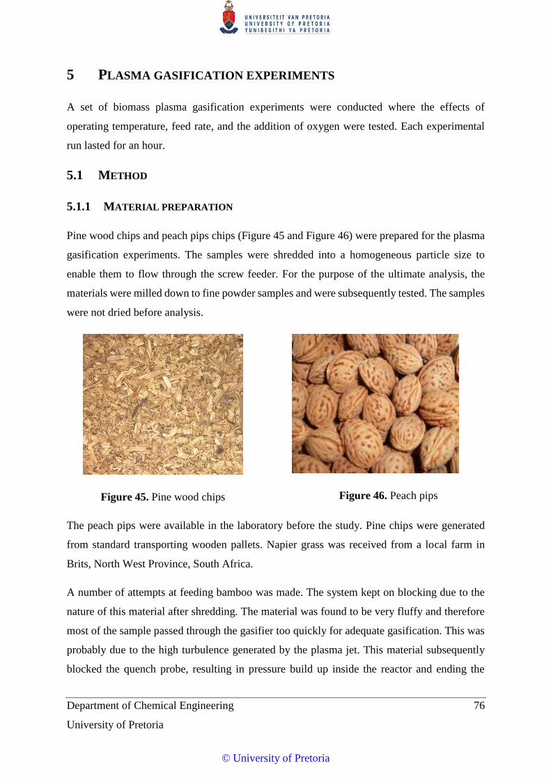
Department of Chemical Engineering 76
University of Pretoria
5 PLASMA GASIFICATION EXPERIMENTS
A set of biomass plasma gasification experiments were conducted where the effects of
operating temperature, feed rate, and the addition of oxygen were tested. Each experimental
run lasted for an hour.
5.1 METHOD
5.1.1 MATERIAL PREPARATION
Pine wood chips and peach pips chips (Figure 45 and Figure 46) were prepared for the plasma
gasification experiments. The samples were shredded into a homogeneous particle size to
enable them to flow through the screw feeder. For the purpose of the ultimate analysis, the
materials were milled down to fine powder samples and were subsequently tested. The samples
were not dried before analysis.
Figure 45. Pine wood chips
Figure 46. Peach pips
The peach pips were available in the laboratory before the study. Pine chips were generated
from standard transporting wooden pallets. Napier grass was received from a local farm in
Brits, North West Province, South Africa.
A number of attempts at feeding bamboo was made. The system kept on blocking due to the
nature of this material after shredding. The material was found to be very fluffy and therefore
most of the sample passed through the gasifier too quickly for adequate gasification. This was
probably due to the high turbulence generated by the plasma jet. This material subsequently
blocked the quench probe, resulting in pressure build up inside the reactor and ending the
© University of Pretoria

Makaringe Chapter 5: Plasma Gasification
Experiments
Department of Chemical Engineering 77
University of Pretoria
experiment prematurely. This problem was also found when feeding Napier grass. It was
concluded that the system was not suitably designed for feeding chipped bamboo and Napier
grass. The plasma gasification work was therefore carried out on only two materials, viz. peach
pips and pine chips.
5.1.2 ULTIMATE ANALYSIS
A general chemical formula for biomass is CxHyOz. In order to determine the values of x, y and
z for each material, an elemental analysis (ultimate analysis) was done. The ultimate analysis
was done on all four materials at the University of Free State. Although Napier grass and
bamboo materials were excluded from the experimental gasification, they were analysed in
order to do the theoretical comparative study as explained earlier. Table 12 shows the ultimate
analysis of the four materials.
Table 12. Ultimate analysis of four biomass material (molar %)
Biomass C H O* N
Bamboo 29.87 46.00 24.12 0
Napier grass 27.35 44.00 28.41 0.24
Peach pips 31.9 45.36 22.64 0.08
Pine tree 29.77 46.52 23.71 0
*Oxygen was determined by difference
5.1.3 SCREW FEEDER CALIBRATION
The screw feeder had to be calibrated for each material. When calibrating the materials, a
specific mass was loaded into the hopper. There is no specification from the suppliers for the
mass for the optimum mas of material inside the hopper for calibration, and for this reason the
same mass material was measured for comparative reasons. A bucket was placed at the outlet
of the hopper. Initially the speed was set at 15.7 rpm and the screw feeder motor was started.
Once the material started to fall into the bucket the timer was started and after 5 min the screw
feeder motor and the timer were stopped. The material was weighed and the mass recorded.
This process was repeated for three more speed settings, i.e. 24.3, 33.0, and 54.5 rpm. The
© University of Pretoria

Makaringe Chapter 5: Plasma Gasification
Experiments
Department of Chemical Engineering 78
University of Pretoria
recorded mass per time interval was plotted against the screw feeder motor speed (Figure 47
and Figure 48). A linear relationship was found and the fitted equation was then used to
calculate a speed setting for a required mass flow rate.
Figure 47. Screw feeder calibration curve for pine wood chips
Figure 48. Screw feeder calibration curve for peach pips
y = 0.0166x + 0.5273
R² = 0.9976
0.5
0.7
0.9
1.1
1.3
1.5
0 10 20 30 40 50 60
Mas
s fl
ow
rat
e (k
g/h
)
Motor speed (rmp)
y = 0.0429x + 0.5279
R² = 0.9996
0.00
2.50
5.00
7.50
10.00
0 50 100 150 200 250
Fee
d R
ate
(kg/h
)
Motor speed (rmp)
© University of Pretoria
Makaringe Chapter 5: Plasma Gasification
Experiments
Department of Chemical Engineering 79
University of Pretoria
5.1.4 LEAK TESTING
The plasma gasification system was tested for any leaks prior to gasification experiments. After
filling the hopper with sufficient material for at least three experimental runs, the whole system
was tightly sealed to make sure that there were no leaks. The leak test was then done by
pressurising the system with nitrogen gas up to a pressure of 1.5 bar absolute. This was above
the operating pressure of the system. A pressure drop was monitored for 5 minutes. If there
was no pressure drop it indicated that the leak rate was small enough to proceed with
experimentation safely. The nitrogen was then flushed out of the system into the building
ventilation by opening the isolation valve after the filter (Figure 25).
5.1.5 PLASMA POWER SUPPLY START UP
Prior to starting the plasma power supply, the cooling water was switched on and the water
flow was recorded. The supply of the plasma gases into the torch was automatically controlled
by the control system of the custom built plasma power supply. The start-up procedures were
pre-set into the controller of the power supply. By pressing the start button the start-up phases
in Table 13 were automatically executed.
Table 13. Plasma power supply start up procedure
Phase no. Description
1 This is a purging phase for argon or nitrogen to ensure that the air is flushed out
of the plasma torch. This phase lasts for 5 seconds.
2 After purging the lines argon is introduced into the torch for few seconds. The
plasma is started during this phase.
3 After the torch is running, stable nitrogen is slowly introduced into the torch
while argon is slowly reduced at the same time. An increase in nitrogen and
decrease in argon happens in parallel until the argon flow is completely stopped.
4 This is an operating phase. The argon flow is now at zero and the torch operates
at a nitrogen flow rate of ~3 kg/h.
© University of Pretoria

Makaringe Chapter 5: Plasma Gasification
Experiments
Department of Chemical Engineering 80
University of Pretoria
The voltage reading depended on the nitrogen flow and is typically between 90 and 100 V. The
current setting is determined by the required temperature of experimentation. A significant
drop in voltage indicates that the torch is faulty and the experiment would need to be stopped
immediately.
5.1.6 BIOMASS FEEDING
It is very important to ensure that the self-cleaning action of the quench probe is working
properly before feeding the biomass into the gasifier. If the quench probe is not functioning
properly the product gas from the reactor is not be cooled sufficiently and results in a prolonged
reaction time which in turn results in the formation of long chain hydrocarbons, not the ideal
products for the purposes of this study.
There is a thermocouple installed in the reactor for reactor temperature monitoring. As backup,
a Minolta Land Cyclops optical pyrometer was used to monitor the reactor temperature. The
pyrometer was focused through a quartz sight glass as described in Chapter 3. Once the reactor
had reached the desired operating temperature (900, 1000 and 1100 °C), the biomass material
feed was started. The screw feeder was set at a desired speed (the feed rates used were 1.00,
1.25 and 1.50 kg/h) according to the calibration curve for the specific material.
5.1.7 SYNGAS SAMPLING
A sampling station was situated outside the gasification containment area as discussed in
Chapter 3. Gas samples were taken every 10 minutes during the course of an experiment. The
gas samples were trapped in the U-tubes (Figure 26) and properly labelled. After each
experimental run these samples were analysed offline by a gas chromatograph (GC).
5.1.8 GASIFICATION EXPERIMENTAL PROCEDURE
5.1.8.1 TEMPERATURE EXPERIMENTS ON PEACH PIPS
The operating temperature is reported to have a significant influence on gasification processes
(Abdoulmoumine et al., 2014; Dufour et al., 2009; Berrueco et al., 2015b; Guo et al., 2014).
The volume of syngas is said to increase with an increase in temperature resulting in a decrease
in char and tar content. At high temperature the tar cracking reaction (Equation 16) is favoured
© University of Pretoria

Makaringe Chapter 5: Plasma Gasification
Experiments
Department of Chemical Engineering 81
University of Pretoria
which further leads to high conversion to gas with low to no tar production (Berrueco et al.,
2015b; Guo et al., 2014; Septien et al., 2012)
COHCHCtarHC yxqp 2)( 16
In order to test the effects of temperature on the plasma gasification process, three different
operating temperatures were investigated in three different experimental runs. The
temperatures were 900, 1000 and 1100 °C. It should be noted that these are the initial reactor
temperature before feeding. During the experimental run the glass hole which was used to
monitor the reactor temperature became dark making it difficult read the temperature using a
pyrometer (the actual temperature readings are shown in Table 14). During experimentation
the reactor temperature was the only variable, with a constant feed rate of 1.25 kg/h and a
constant equivalence ratio (defined as the ratio of actual oxidant supplied to stoichiometric
oxidant required for complete combustion, on a dry ash free (daf) basis) of zero. In most studies
the effect of temperature is tested with an ER between 0.25 and 0.3. The electrical power input
into the plasma torch to reach a reactor temperature of 900, 1000 and
1100 °C were 12.7 ±1.4, 12.8 ±1.8 and 13.3 ±2.1 kW respectively.
5.1.8.2 FEEDING RATE EXPERIMENTS ON PEACH PIPS
High feed rates result in high gas yields, but lead to lower gas quality and high tar yield (Guo
et al., 2014). In this study the feed rate was evaluated to determine its effect on biomass
conversion as well as syngas concentration. Three different feed rates of 1.0, 1.25 and 1.5 kg/h
were tested. A feed rate of 1.0 kg/h corresponded to the minimum setting of the feeder. When
a feed rate of >1.5 kg/h was used, the feed material filled the plasma reactor, preventing
efficient gasification process. Therefore the feed rate tests were limited to this range. The tests
were done using a constant temperature of 1000 °C (the initial reactor temperature) with an
equivalence ratio (ER) of zero. The residue remaining after every experimental run were
measured and compared. The quality of the syngas was also analysed for each experimental
run.
© University of Pretoria

Makaringe Chapter 5: Plasma Gasification
Experiments
Department of Chemical Engineering 82
University of Pretoria
5.1.8.3 EQUIVALENCE RATIO EXPERIMENTS ON PINE WOOD CHIPS
The equivalence ratio quantifies the oxygen feed into the process (Guo et al., 2014). It is
defined as the ratio of actual oxidant supplied to stoichiometric oxidant required for complete
combustion on a dry ash free (daf) basis (Equation 17).
17
where Φm,oxy is the oxygen flow rate and Φm,fuel is the biomass flow rate. In general, full
gasification occurs at an ER ~ 0.25. By way of illustration see point G in Figure 49. The exact
temperature value may not be realistic for plasma processes, since the illustration is from
general gasification literature.
Figure 49. The equivalence ratio diagram (Reed and Desrosiers)
The effect of equivalence ratio on biomass plasma gasification was studied by varying the
amount of oxygen flow into the reactor in three sets of experiments. Biomass composition is
required when calculating the equivalence ratio. In this case the chemical formula of pine wood
was calculated from the ultimate analysis in Table 12 and was found to be CH1.6O0.8. The
stoichiometric oxygen/fuel ratio was determined from a complete combustion reaction
(Equation 18).
stoichfuelmoxym
actualfuelmoxymER
,,
,,
© University of Pretoria
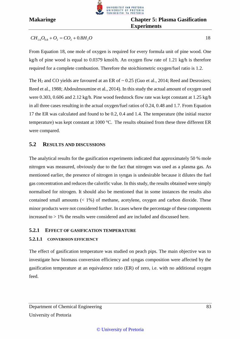
Makaringe Chapter 5: Plasma Gasification
Experiments
Department of Chemical Engineering 83
University of Pretoria
OHCOOOCH 2228.06.1 8.0 18
From Equation 18, one mole of oxygen is required for every formula unit of pine wood. One
kg/h of pine wood is equal to 0.0379 kmol/h. An oxygen flow rate of 1.21 kg/h is therefore
required for a complete combustion. Therefore the stoichiometric oxygen/fuel ratio is 1.2.
The H2 and CO yields are favoured at an ER of ~ 0.25 (Guo et al., 2014; Reed and Desrosiers;
Reed et al., 1988; Abdoulmoumine et al., 2014). In this study the actual amount of oxygen used
were 0.303, 0.606 and 2.12 kg/h. Pine wood feedstock flow rate was kept constant at 1.25 kg/h
in all three cases resulting in the actual oxygen/fuel ratios of 0.24, 0.48 and 1.7. From Equation
17 the ER was calculated and found to be 0.2, 0.4 and 1.4. The temperature (the initial reactor
temperature) was kept constant at 1000 °C. The results obtained from these three different ER
were compared.
5.2 RESULTS AND DISCUSSIONS
The analytical results for the gasification experiments indicated that approximately 50 % mole
nitrogen was measured, obviously due to the fact that nitrogen was used as a plasma gas. As
mentioned earlier, the presence of nitrogen in syngas is undesirable because it dilutes the fuel
gas concentration and reduces the calorific value. In this study, the results obtained were simply
normalised for nitrogen. It should also be mentioned that in some instances the results also
contained small amounts (< 1%) of methane, acetylene, oxygen and carbon dioxide. These
minor products were not considered further. In cases where the percentage of these components
increased to > 1% the results were considered and are included and discussed here.
5.2.1 EFFECT OF GASIFICATION TEMPERATURE
5.2.1.1 CONVERSION EFFICIENCY
The effect of gasification temperature was studied on peach pips. The main objective was to
investigate how biomass conversion efficiency and syngas composition were affected by the
gasification temperature at an equivalence ratio (ER) of zero, i.e. with no additional oxygen
feed.
© University of Pretoria

Makaringe Chapter 5: Plasma Gasification
Experiments
Department of Chemical Engineering 84
University of Pretoria
In order to determine conversion efficiency achieved, the particulates remaining after each
temperature test were collected from the reactor, the gas outlet pipe, the knock-out pot, and the
filter (Chapter 3). These particulates were weighed and total conversion efficiency was
calculated by subtracting the total remaining particulates from the total biomass fed into the
system. The conversion efficiency (in wt %) was then plotted against the operating temperature
(Figure 50).
Figure 50.Temperature vs conversion using peach pips as feed
Conversion efficiency slightly increased with an increase in the gasification temperature
(Figure 50). This is in agreement with literature. At high temperatures products of endothermic
reactions are favoured (Lv et al., 2004). Since the tests were done in the absence of an oxidant,
the water-gas and Boudouard reactions, Equation 1 & 5 which are endothermic were favoured,
contributing to an increase in H2 and CO formation and leading to a decrease in char
(Berrueco et al., 2015b; Abdoulmoumine et al., 2014). The conversion achieved for the
gasification temperatures of 900, 1000 and 1100 °C were 72.5, 73 and 74 % respectively.
50
60
70
80
90
850 900 950 1000 1050 1100 1150
Con
ver
sion
α (
wt.
%)
Temperature (°C)
© University of Pretoria
Makaringe Chapter 5: Plasma Gasification
Experiments
Department of Chemical Engineering 85
University of Pretoria
5.2.1.2 SYNGAS CONCENTRATION
Figure 51 shows the effect of temperature on CO and H2 formation. As already explained
earlier, components such as CO2 and CH4 are not shown in this graph since their concentration
were less than 1 % mol. From this observation it is clear that the CO/H2 ratios were ~ 1 in all
three cases (i.e. 1.03 at 900 °C, 1.026 at 1000 °C and 0.98 at 1100 °C). As expected the
concentration of H2 slightly increased from 49 to 51 % mole when the temperature was
increased from 900 to 1100 °C. This was due to the water-gas reaction. On the other hand the
concentration of CO slightly decreased with an increase in temperature. The trend of CO
formation varies in different studies. It was found to increase with temperature between 700
and 800 °C, then remained constant between 800 and 1000 °C in the absence of an oxidant
(Dufour et al., 2009). It was found to slightly decrease with an increase in temperature between
700 and 800 °C and sharply increase between 800 and 850 °C at an ER ~ 0.31
(Berrueco et al., 2015b). In another study it was found to increase with an increase in
temperature between 800 and 1100 °C when the ER ~ 0.25 (Abdoulmoumine et al., 2014).
These variations may have been caused by the possibilities of many reactions during
gasification. Depending on the conditions inside the reactor at the point when the samples were
taken, one reaction which is favourable or unfavourable to the formation of CO may have taken
place.
Figure 51. Product yield vs temperature using peach pips
35
40
45
50
55
800 850 900 950 1000 1050 1100 1150
Mole
per
cen
tage
(%)
Temperature (°C)
H2
CO
© University of Pretoria

Makaringe Chapter 5: Plasma Gasification
Experiments
Department of Chemical Engineering 86
University of Pretoria
5.2.1.3 ENERGY BALANCE
The mass and energy flows for peach pips gasification under a constant feed rate of 1.25 kg/h
and different gasification temperatures of 900, 1000 and 1100 °C are shown in Table 14. From
the literature, the calorific value of peach pip was found to be 19.4 kJ/g, producing (6.8 kW for
a feed rate of 1.25 kg/h (Parikh et al., 2005).
Table 14. Calorific value of syngas produced from gasification of peach pips at different
temperatures
Torch power
(kW)
Temperature
(°C)
Syngas
(kg/h)
H2
(mol %)
CO
(mol %)
LHVsyngas
(kW)
LHVsyngas
(kJ/g)
12.7 ±1.4 912.9 0.910 51 49 4.47 17.68
12.8 ± 1.9 934.7 0.913 51 49 4.48 17.66
13.0 ± 2.1 1097 0.925 49 51 4.46 17.35
It is observed from Table 14 that the calorific values of the syngas obtained at different
gasification temperatures were almost equal, at 4.5 kW. Approximately 66% of the energy
contained in the feed material was released as syngas. The rest of the energy (~34 %) remain
in the solid residues (char). This was in agreement with the mass conversion results.
Roughly 35 % of the energy input into the system as electrical energy to run the torch, is
recovered as the chemical energy content of the syngas. Sensible heat losses to the various
reactor and torch components are given in Table 15. The torch has a very low energy efficiency.
Commercially available non-transfer arc plasma torches have energy efficiencies of ~ 65%
(Hrabovsky et al., 2006). In this system the efficiency of the torch was found for be ~ 32 %.
The main reason for this was the fact the gasification reactor was not optimised to shield the
anode housing from the heat radiation from the reactor. As a result 66 % of the energy supplied
into the plasma torch was lost through anode cooling. The sensible heat content of the syngas
constitutes 16 % of the energy input, while reactor losses constitute 18 %. Obviously a net
© University of Pretoria

Makaringe Chapter 5: Plasma Gasification
Experiments
Department of Chemical Engineering 87
University of Pretoria
positive amount of energy is desired. To achieve this a careful thermal and mechanical redesign
of the system is required.
Table 15: Average power losses to various water-cooled torch and reactor components
Component Power
losses (%)
Cathode 2
Anode 66
Inner quench 10
Outer quench 6
Reactor wall 12
Reactor
flange
4
5.2.2 EFFECT OF FEED RATE
5.2.2.1 CONVERSION EFFICIENCY
The effect of feed rate on gas and char yield was investigated for peach pips. In some gasifiers
a high feed rate is known to be beneficial for increasing product yield (Guo et al., 2014; Lv et
al., 2007). However, it could reduce product quality due to higher gas yield and shorter
residence leading to higher tar yield.
The results in Figure 52 shows no clear trend in the range of feed rates investigated. It decreased
from 78 wt % to 73 wt % when the feed rate was increased from 1.00 to 1.25 kg/h. It then
increased to 78 wt % when the feed rate was increased from 1.25 to 1.50 kg/h. It should be
noted that these tests were done in the absence of an oxidant (i.e. ER ~ 0) at a constant reactor
temperature (before feeding) of 1000 °C. In general conversion is expected increase with a
decrease in feed rate due to the effective mass and heat transfer at lower feeding rates. Due to
the turbulent nature inside the plasma reactor, it can be assumed that some very fine particles
escape the reactor before they can be gasified. This could have caused the conversion at 1.25
kg/h to be lower than that at 1.50 kg/h. Another scenario could be that the tested feed rates
© University of Pretoria

Makaringe Chapter 5: Plasma Gasification
Experiments
Department of Chemical Engineering 88
University of Pretoria
were too close to one another due to the system limitations already explained.
Figure 52. Feed rate vs conversion curve
5.2.2.2 HYDROGEN AND CARBON MONOXIDE CONCENTRATION
The relative H2 and CO concentrations were also not markedly affected by an increase in feed
rate under these conditions. The concentration of these gases were almost constant at all three
tested feed rates (i.e. 1.00, 1.25 and 1.50 kg/h) and a CO/H2 ratio of ~ 1 was achieved in all
three cases, Figure 53.
50
60
70
80
90
100
0.9 1.05 1.2 1.35 1.5
Conver
sion (
wt.
%)
Feed rate (kg/h)
© University of Pretoria

Makaringe Chapter 5: Plasma Gasification
Experiments
Department of Chemical Engineering 89
University of Pretoria
Figure 53. Product yield vs feed rate using peach pips as feed
At a feed rate between 1.00 and 1.25 kg/h, the H2 concentration slightly decreased from 50.72
to 49.34 % mole. It then slightly increased to 50 % mole when the feed rate was increased to
1.50 kg/h. The CO concentration, on the other hand had an opposite trend to H2 concentration.
It slightly increased from 49.28 to 50.66 % mole between 1.00 and 1.25 kg/h then slightly
decreased to 50 % mole at 1.50 kg/h.
5.2.2.3 ENERGY BALANCE
The calorific values of the syngas produced at different feed rates and constant temperature of
1000 °C are shown in Table 16 . The maximum power yields calculated from the enthalpy of
combustion of peach pips for the feed rates of 1.0, 1.25 and 1.5 kg/h, are 5.44, 6.80 and 8.70
kW respectively.
30
35
40
45
50
55
60
0.9 1 1.1 1.2 1.3 1.4 1.5 1.6
Mo
le p
erc
en
tage
(%
)
Feed rate (kg/h)
H2
CO
© University of Pretoria

Makaringe Chapter 5: Plasma Gasification
Experiments
Department of Chemical Engineering 90
University of Pretoria
Table 16. Calorific values of syngas produced from gasification of peach pips at different
feed rates
Feed rate
(kg/h)
Syngas
(kg/h)
H2
(mol %)
CO
(mol %)
LHVsyngas
(kW)
LHVsyngas
(kJ/g)
1 0.78 51 49 3.85 17.77
1.25 0.91 49 51 4.37 17.36
1.5 1.17 50 50 5.69 17.50
Comparing these values to the syngas energy flow in Table 16 that 70.8, 64.2 and 65.4 % of
the energy contained in the feed material was released into the syngas for the feed rate of 1,
1.25 and 1.5 kg/h respectively. A higher energy yield is thus obtained at higher feed rates, but
at the expense of conversion efficiency. This suggests that the gasification systems may be
more economical at larger scales. The mixture of the syngas and the nitrogen exiting through
the quench probe gas was cooled to ~ 29°C.
5.2.3 EFFECT OF EQUIVALENCE RATIO
5.2.3.1 CONVERSION EFFICIENCY
The conversion efficiency of pine wood versus the ER curve is shown Figure 54.
© University of Pretoria
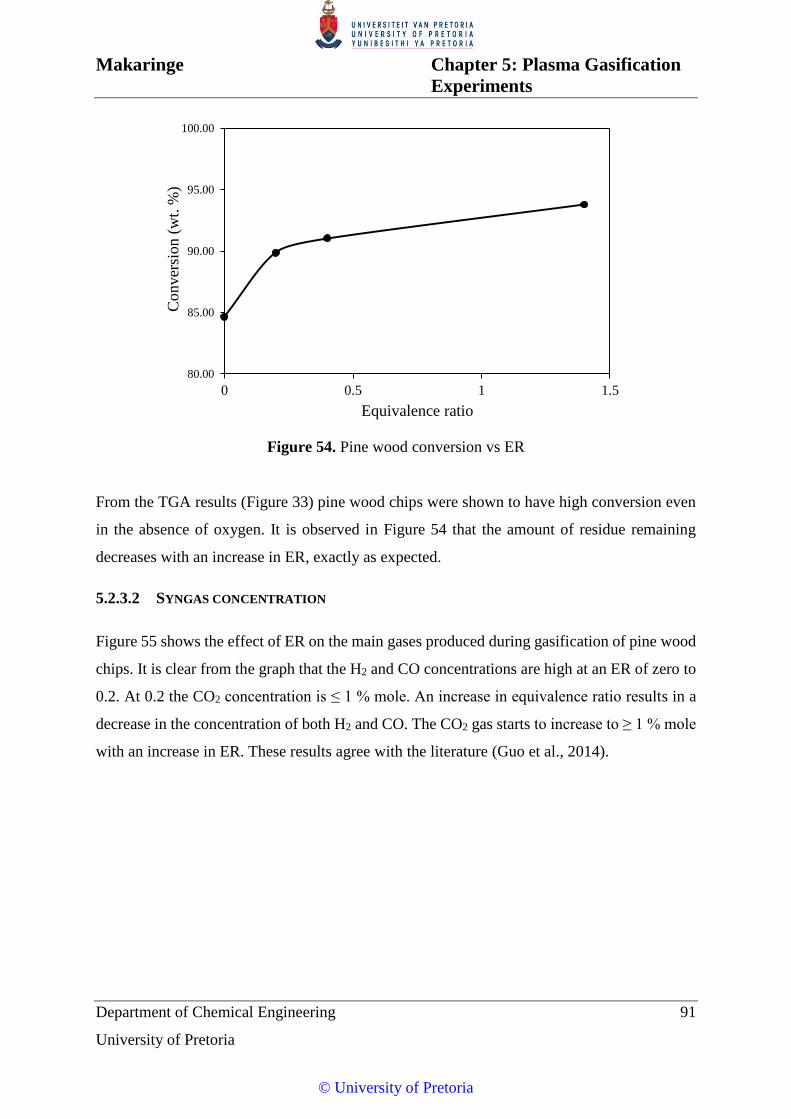
Makaringe Chapter 5: Plasma Gasification
Experiments
Department of Chemical Engineering 91
University of Pretoria
Figure 54. Pine wood conversion vs ER
From the TGA results (Figure 33) pine wood chips were shown to have high conversion even
in the absence of oxygen. It is observed in Figure 54 that the amount of residue remaining
decreases with an increase in ER, exactly as expected.
5.2.3.2 SYNGAS CONCENTRATION
Figure 55 shows the effect of ER on the main gases produced during gasification of pine wood
chips. It is clear from the graph that the H2 and CO concentrations are high at an ER of zero to
0.2. At 0.2 the CO2 concentration is ≤ 1 % mole. An increase in equivalence ratio results in a
decrease in the concentration of both H2 and CO. The CO2 gas starts to increase to ≥ 1 % mole
with an increase in ER. These results agree with the literature (Guo et al., 2014).
80.00
85.00
90.00
95.00
100.00
0 0.5 1 1.5
Conver
sion (
wt.
%)
Equivalence ratio
© University of Pretoria

Makaringe Chapter 5: Plasma Gasification
Experiments
Department of Chemical Engineering 92
University of Pretoria
Figure 55. Product yield vs ER
At an ER value of 1, full combustion and maximum concentrations of CO2 and H2O are
expected as the main products. The gas samples in this study were not analysed for H2O, and
the results were simply normalised with respect the gases that were analysed for. It is clear at
1 and higher, significant concentrations of CO and H2 are still present. Mass transfer and kinetic
effects are undoubtedly responsible. Nevertheless, the overall observed trend is the expected
behaviour.
5.2.3.3 ENERGY BALANCE
The calorific content of syngas produced at different ER values, and a constant temperature
and constant feed rate of 1000°C and 1.25 kg/h respectively, are shown in Table 17. Pine wood
has a combustion enthalpy of 19.38 kJ/g (Cuiping et al., 2004) Therefore a feed rate of 1.25
kg/h has a maximum energy flow of 6.7 kW.
0
10
20
30
40
50
60
70
0 0.25 0.5 0.75 1 1.25 1.5
Co
nce
ntr
atio
n (
mo
le %
)
Equivalence ratio
H2
CO
CO2
O2
© University of Pretoria

Makaringe Chapter 5: Plasma Gasification
Experiments
Department of Chemical Engineering 93
University of Pretoria
Table 17 Calorific values of syngas produced for gasification of pine wood at different ER
Equivalence
ratio
Syngas
(kg/h)
H2
(mol %)
CO
(mol %)
CO2
(mol %)
O2
(mol %)
LHVsyngas
(kW)
LHVsyngas
(kJ/g)
0 1.06 48.7 51.3 <1 <1 5.04 17.14
0.2 1.12 48.3 51.8 <1 <1 5.31 17.03
0.4 1.14 45.3 49.0 5.7 <1 5.37 16.97
1.4 1.17 8.9 22.3 62.5 6.4 0.77 2.35
It is evident from Table 16 that the calorific value of syngas increased with an increase in ER,
up to 0.4. When the ER was increased to 1.4 the caloric value of the syngas decreased
significantly to 0.77 kW. This is due to the fact that the combustible gases (CO and H2) were
decreased while the CO2 was increased. As already mentioned pine wood has high conversion
efficiency, leading to the calorific values obtained during the gasification of pine to be higher
than that obtained during the gasification of peach pips even at an equivalence ratio of zero.
Comparing the enthalpy of combustion of syngas to that of feed material (pine wood) for a feed
rate of 1.25 kg/h, it was found that 75.2, 79.2, 80.1 and 11.5 % of the energy contained in the
feed material was released to syngas for the equivalence ratios of 0, 0.2, 0.4 and 1.4
respectively.
5.3 CONCLUSION
Initially the plasma gasification system was to be investigated using the four different biomass
types. However the test work was carried out using only two materials, viz. peach pips and
pine wood chips. This was due to the very light nature and low density of the bamboo and
Napier grass. The design of the plasma gasification system was unable to accommodate these
low density materials. This resulted in blockages of the system and thereby ending the
experiment prematurely. It could be concluded that this system is not desirable for low density
material.
© University of Pretoria

Makaringe Chapter 5: Plasma Gasification
Experiments
Department of Chemical Engineering 94
University of Pretoria
The parameters that were evaluated were the gasification temperature, feed rate and the ER.
Operating temperatures of 900, 1000 and 1100 °C, feed rates of 1.00, 1.25, and 1.50 kg/h, and
the ER values of zero, 0.2, 0.4 and 1.4 were studied. The gasification results indicated that high
temperature increased conversion efficiency as the amount of the residue decreased with an
increase in gasification temperature. However the product concentrations were not affected by
an increase in gasification temperature, the concentration of H2 and CO were mostly high due
to the fact that at high temperatures the water-gas shift and the Boudouard reactions were
favoured. The CO/H2 ratios of ~ 1 were achieved in all three gasification temperatures.
However H2 concentration seemed to increase with an increase in temperature while CO
concentration decreased with an increase in temperature.
The tested feed rates were found to have a negligible influence on conversion efficiency as well
as on product concentration. Conversion efficiency slightly fluctuated with an increase in feed
rate. This could be linked to particle size of the feed stock, but was not confirmed. If finer
particles are available in the hopper during the gasification test at a specific feed rate, the finer
particles could escape the reactor before being gasified.
The use of oxidant has a significant influence in the overall gasification process as expected.
Operating the plasma gasification system with zero ER resulted in a CO/H2 ratio of ~ 1. A
conversion efficiency of ~ 85 % was achieved on pine wood. An ER of 0.2 increased
conversion efficiency to ~ 90 % while keeping the CO/H2 ratio almost the same. A conversion
of ~ 91% was achieved when the ER was increased to 0.4. However, the CO2 concentration
started to increase to above 1% mole. At an ER of 1.4, CO2 production increased significantly
to ~ 68 % mol. It can be concluded that an ER between 0.2 and 0.4 is favourable for the biomass
plasma gasification process. This agrees with the literature.
The efficiency of converting the electrical energy used for gasification to the chemical energy
yield from the syngas, is 30 % to 40 %. The main heat losses is via the torch anode, and thought
to be due to the absence of radiation shielding. This may be corrected by a redesign; also the
efficiency is expected to increase for larger gasification systems.
© University of Pretoria

Department of Chemical Engineering 95
University of Pretoria
6 CONCLUSION AND RECOMMENDATIONS
For both TGA and plasma experimental tests, the highest conversion achieved for peach pips
under inert conditions was ~ 78 wt %, while that for pine wood under similar conditions was ~
85 wt %. The TGA results also indicated the importance of heating rate, with higher heating
rates is resulting in higher conversion of biomass to gas. High conversion efficiencies were
achieved at higher heating rate in all materials. The heating rate with plasma gasification cannot
be controlled; however plasma processes are generally known for their high heating rates,
which makes them ideal for gasification processes. One would expect higher conversion for
the plasma than for the TGA runs. The fact that this was not observed can be ascribed to
uncontrolled dwell time of the feed in the reactor, resulting in the conversion reactions not
going to completion.
High temperatures favour the product of the endothermic reactions leading to an increase in
the formation of CO and H2. As a consequence the plasma experiments yielded predominantly
CO and H2, except for high ER values. The plasma gasification results indicated an ER between
0.2 and 0.4 to be optimum.
Particle sizes were found to have a crucial role when investigating the effect of feed rate in this
system. It is important to use millimetre size particle sizes and avoid the presence of fine
particle with low density when testing the effect of feed rate. It was established that low density
particles easily escape the reactor without being gasified due to the turbulence inside the
reactor.
For this reactor system, the results indicated that more energy has to be put into the gasification
process than can be recovered from the combustion of the syngas produced. Overall
efficiencies range between 30 and 40 %. The highest energy loss in the system is via the torch
anode. More than 60 % of the power is lost this way, resulting in a nominal torch efficiency of
~30 %. Non-transferred torches are expected to have efficiencies higher than 60 %. The high
anode power losses is most probably attributable to radiative heat impinging on the torch from
the gasification reactor chamber.
The main recommendation is that the free-standing efficiency of the torch should be measured,
i.e. away from the gasification reactor. If it is indeed low, the torch should be optimised to
© University of Pretoria

Makaringe Chapter 6: Conclusion and
Recommendations
Department of Chemical Engineering 96
University of Pretoria
obtain an efficiency of at least 60%. If the torch efficiency is not the problem, then a redesign
to protect the torch from reactor radiation should be implemented.
© University of Pretoria

Department of Chemical Engineering 97
University of Pretoria
7 FUTURE WORK: ORGANIC CHEMICAL WASTE PLASMA
GASIFICATION
7.1 CHEMICAL WASTE PLASMA TREATMENT (LIPF6)
Initially plasma technology at Necsa was developed for waste reduction, especially radiological
waste. However, due to the safety issues concerning the handling radioactive material, the
technology is being tested on non-radioactive waste such as biomass. However there is other
conventional chemical waste generated at Necsa whose disposal is of concern. Generally any
chemical waste generated during chemical processes needs to be treated before it can be
disposed of in a land fill site. Some chemical waste needs special treatment.
A lot of liquid waste is generated during the production of lithium hexafluorophosphate (LiPF6)
in the fluorine laboratory at Necsa. As a first step towards the treatment of this waste,
poly(methyl methacrylate) (PMMA) polymer is used to solidify for solidifying the solution.
The solidified waste is carbon rich, therefore converting it to energy through plasma
gasification was considered a viable treatment method. This would solve the waste disposal
problem while in turn producing syngas. This work was conducted as a preliminary study.
7.1.1 BRIEF BACKGROUND ON LITHIUM HEXAFLUOROPHOSPHATE
Lithium hexafluorophosphate (LiPF6) serves as an electrolyte in lithium ion batteries. LiPF6 is
used mainly because it is easily soluble in various solvents, has a high electrical conductivity
in non-aqueous solution, and has high electrochemical stability. Lithium hexafluorophosphate
electrolytes are prepared by dissolving a LiPF6 organic complex or pure LiPF6 salt in a suitable
electrolyte solvent, such as propylene carbonate.
Lithium hexafluorophosphate waste was produced in the laboratory at Necsa. The LiPF6 was
further dissolved in propylene carbonate in for various tests, including stability as an electrolyte
component. This resulted in generation of liquid waste. This waste is very toxic and harmful
to the environment, thus needs special treatment and disposal procedures. The plasma waste
treatment system was therefore considered and then used as a treatment method.
© University of Pretoria

Makaringe Chapter 7: Future work
Department of Chemical Engineering 98
University of Pretoria
7.1.2 WASTE SOLIDIFICATION PROCESS
Lithium hexafluorophosphate (LiPF6) dissolves in several solvents, for example, propylene
carbonate, resulting in a LiPF6 solution which may be classified as waste after use in research
facilities. This waste may be dissolved in small pieces of PMMA, such as beads or powders.
By controlling the volume of the liquid used and allowing the material to settle for
approximately two weeks, solid PMMA encapsulated waste was generated (Figure 56).
Poly(methyl methacrylate) used for this purpose was purchased from Sigma-Aldrich.
Figure 56. PMMA encapsulated waste
7.1.3 EXPERIMENTAL METHOD
The screw feeder was calibrated for this specific material. The operating parameters were as
follows: a feed rate of 1.00 kg/h and a temperature of 1000 °C in the absence of an oxidant. A
solid block of PMMA encapsulated LiPF6 waste was chopped into smaller piece to enable easy
feeding. These pieces were loaded into the hopper. The same operating procedures as in
Chapter 5 were followed. The system was operated for an hour. During this process two
samples were taken using U-tubes, and submitted analysis.
7.1.4 RESULTS AND DISCUSSIONS
The gas samples were analysed for syngas product using a GC. As for the biomass gasification
case, the results were normalised for nitrogen. The normalised results were found to contain
53 % mole H2 and 47% mole CO. The residues remaining after the tests were
~ 5 wt % in the form of fine ash. The residues were not analysed for traces of lithium due to
the lack of an appropriate analytical instrument. Also the column used in the GC couldn’t be
used for fluorine compounds.
© University of Pretoria

Makaringe Chapter 7: Future work
Department of Chemical Engineering 99
University of Pretoria
7.1.5 CONCLUSION
The preliminary work that was done to demonstrate the use of plasma gasification as a chemical
waste treatment method indicated that the chemical waste (LiPF6) was successfully treated, and
in turn produced syngas. In future more work still needs to be done so that the residues can be
analysed for traces of lithium. The gases produced also need to be analysed for fluorine
compounds before they can be considered safe to be labelled as syngas.
© University of Pretoria

Department of Chemical Engineering 100
University of Pretoria
8 REFERENCES
Abdoulmoumine N, Kulkarni A and Adhikari S. (2014) Effects of Temperature and
Equivalence Ratio on Pine Syngas Primary Gases and Contaminants in a Bench-Scale
Fluidized Bed Gasifier. Industrial & Engineering Chemistry Research 53: 5767-5777.
Bassilakis R, Carangelo RM and Wojtowicz MA. (2001) TG-FTIR analysis of biomass
pyrolysis. Fuel 80: 1765-1786.
Berndes Gr, Hoogwijk M and van den Broek R. (2003) The contribution of biomass in the
future global energy supply: a review of 17 studies. Biomass and Bioenergy 25: 1-28.
Berrueco C, Recari J, Abelló S, et al. (2015a) Experimental investigation of solid recovered
fuel (SRF) gasification: Effect of temperature and equivalence ratio on process performance
and release of minor contaminants. Energy and Fuels 29: 7419-7427.
Berrueco C, Recari J, Abelló S, et al. (2015b) Experimental investigation of solid recovered
fuel (SRF) gasification: Effect of temperature and equivalence ratio on process performance
and release of minor contaminants. Energy & fuels 29: 7419-7427.
Boulos MI. (1991) Thermal plasma processing. IEEE Transactions on Plasma Science 19:
1078-1089.
Boulos MI, Fauchais P and Pfender E. (2013) Thermal Plasmas: Fundamentals and
Applications: Springer Science & Business Media.
Bridgwater AV. (2003) Renewable fuels and chemicals by thermal processing of biomass.
Chemical Engineering Journal 91: 87-102.
Bridgwater AV. (2012) Review of fast pyrolysis of biomass and product upgrading. Biomass
and Bioenergy 38: 68-94.
Brown ME, Maciejewski M, Vyazovkin S, et al. (2000) Computational aspects of kinetic
analysis: Part A: The ICTAC kinetics project-data, methods and results. Thermochimica Acta
355: 125-143.
Camacho SL. (1996) Plasma pyrolysis and vitrification of municipal waste. U.S. Patent
© University of Pretoria

Makaringe Chapter 8: References
Department of Chemical Engineering 101
University of Pretoria
5,544,597. Raleigh, N.C: Plasma Technology Corporation.
Channiwala SA and Parikh PP. (2002) A unified correlation for estimating HHV of solid, liquid
and gaseous fuels. Fuel 81: 1051-1063.
Chen G, Andries J, Luo Z, et al. (2003) Biomass pyrolysis/gasification for product gas
production: the overall investigation of parametric effects. Energy Conversion and
Management 44: 1875-1884.
Cuiping L, Chuangzhi W, Yanyongjie, et al. (2004) Chemical elemental characteristics of
biomass fuels in China. Biomass and Bioenergy 27: 119-130.
Demirbas A. (2004) Combustion characteristics of different biomass fuels. Progress in Energy
and Combustion Science 30: 219-230.
Devi L, Ptasinski KJ and Janssen FJJG. (2003) A review of the primary measures for tar
elimination in biomass gasification processes. Biomass and Bioenergy 24: 125-140.
Dighe SV, Darr MF, Martorell IA, et al. (2010) Plasma gasification reactor. US2010/0199556
A1. Madisos, US: Westinghouse Plasma Corporation.
Duan Z and Heberlein J. (2002) Arc instabilities in a plasma spray torch. Journal of Thermal
Spray Technology 11: 44-51.
Dufour A, Girods P, Masson E, et al. (2009) Synthesis gas production by biomass pyrolysis:
Effect of reactor temperature on product distribution. International Journal of Hydrogen
Energy 34: 1726-1734.
Fauchais P and Vardelle A. (1997) Thermal plasmas. IEEE transactions on plasma science 25:
1258-1280.
Favalli R and Szente R. (1998) Physical and mathematical modeling of non transferred plasma
torches. Brazilian journal of physics 28: 25-34.
Galeno G, Minutillo M and Perna A. (2011) From waste to electricity through integrated
plasma gasification/fuel cell (IPGFC) system. International Journal of Hydrogen Energy 36:
1692-1701.
© University of Pretoria

Makaringe Chapter 8: References
Department of Chemical Engineering 102
University of Pretoria
Gašparovič L, Koreňová Z and Jelemenský Ľ. (2010) Kinetic study of wood chips
decomposition by TGA. Chemical Papers 64: 174-181.
Gassner M and Maréchal F. (2009) Thermo-economic process model for thermochemical
production of Synthetic Natural Gas (SNG) from lignocellulosic biomass. Biomass and
Bioenergy 33: 1587-1604.
Ghetti P, Ricca L and Angelini L. (1996) Thermal analysis of biomass and corresponding
pyrolysis products. Fuel 75: 565-573.
Gomez E, Rani DA, Cheeseman CR, et al. (2009) Thermal plasma technology for the treatment
of wastes: A critical review. Journal of Hazardous Materials 161: 614-626.
Guo F, Dong Y, Dong L, et al. (2014) Effect of design and operating parameters on the
gasification process of biomass in a downdraft fixed bed: An experimental study. International
Journal of Hydrogen Energy 39: 5625-5633.
Han J and Kim H. (2008) The reduction and control technology of tar during biomass
gasification/pyrolysis: an overview. Renewable and Sustainable Energy Reviews 12: 397-416.
Hlina M, Hrabovsky M, Kavka T, et al. (2011) Tar measurement in synthetic gas produced by
plasma gasification by solid phase microextraction (SPME). ISPC Conference. 24-29 July,
Philadelphia, USA.
Hrabovsky M, Kopeckykopecky V, Sember V, et al. (2006) Properties of hybrid water/gas DC
arc plasma torch. IEEE Transactions on Plasma Science 34: 1566-1575.
Hui Z, Huaxiao Y, Mengmeng Z, et al. (2010) Pyrolysis characteristics and kinetics of
macroalgae biomass using thermogravimetric analyzer. Proc World Acad Sci Eng Technol 65:
1161-1166.
Inczedy J, Lengyel T, Ure A, et al. (1998) Compendium of Analytical Nomenclature, Oxford:
Blackwell.
Khawam A and Flanagan DR. (2005) Role of isoconversional methods in varying activation
energies of solid-state kinetics: I. Isothermal kinetic studies. Thermochimica Acta 429: 93-102.
© University of Pretoria

Makaringe Chapter 8: References
Department of Chemical Engineering 103
University of Pretoria
Khawam A and Flanagan DR. (2006) Solid-state kinetic models: basics and mathematical
fundamentals. The Journal of Physical Chemistry B 110: 17315-17328.
Kim J, Yun S and Ounaies Z. (2006) Discovery of cellulose as a smart material.
Macromolecules 39: 4202-4206.
Klinger L, Vos JB and Appert K. (2003) High-resolution CFD simulation of a plasma torch in
3 dimensions. Infoscince, (No. CRPP-REPORT-2003-024).
Kögel-Knabner I. (2002) The macromolecular organic composition of plant and microbial
residues as inputs to soil organic matter. Soil Biology and Biochemistry 34: 139-162.
Kumar A, Wang L, Dzenis YA, et al. (2008) Thermogravimetric characterization of corn stover
as gasification and pyrolysis feedstock. Biomass and Bioenergy 32: 460-467.
Lee M-K, Tsai W-T, Tsai Y-L, et al. (2010) Pyrolysis of napier grass in an induction-heating
reactor. Journal of analytical and applied pyrolysis 88: 110-116.
Lemmens B, Elslander H, Vanderreydt I, et al. (2007) Assessment of plasma gasification of
high caloric waste streams. Waste Management 27: 1562-1569.
Luche J, Falcoz Q, Bastien T, et al. (2012) Plasma treatments and biomass gasification. IOP
Conference Series: Materials Science and Engineering. IOP Publishing, 012011.
Lv P, Yuan Z, Ma L, et al. (2007) Hydrogen-rich gas production from biomass air and
oxygen/steam gasification in a downdraft gasifier. Renewable Energy 32: 2173-2185.
Lv PM, Xiong ZH, Chang J, et al. (2004) An experimental study on biomass air–steam
gasification in a fluidized bed. Bioresource Technology 95: 95-101.
Mansaray KG and Ghaly AE. (1999) Determination of kinetic parameters of rice husks in
oxygen using thermogravimetric analysis. Biomass and Bioenergy 17: 19-31.
McKendry P. (2002a) Energy production from biomass (part 1): overview of biomass.
Bioresource Technology 83: 37-46.
McKendry P. (2002b) Energy production from biomass (part 3): gasification technologies.
Bioresource Technology 83: 55-63.
© University of Pretoria
Makaringe Chapter 8: References
Department of Chemical Engineering 104
University of Pretoria
Meng J and Dong X. (2011) Numerical simulation and analysis on jet characteristics of
combined plasma arc. Open Mechanical Engineering Journal 5: 78-86.
Meng X, de Jong W, Fu N, et al. (2011) Biomass gasification in a 100 kWth steam-oxygen
blown circulating fluidized bed gasifier: Effects of operational conditions on product gas
distribution and tar formation. Biomass and Bioenergy 35: 2910-2924.
Mui ELK, Cheung WH, Lee VKC, et al. (2008) Kinetic study on bamboo pyrolysis. Industrial
& Engineering Chemistry Research 47: 5710-5722.
Murphy A. (2001) Thermal plasmas in gas mixtures. Journal of Physics D: Applied Physics
34: R151.
Nahman A, de Lange W, Oelofse S, et al. (2012) The costs of household food waste in South
Africa. Waste Management 32: 2147-2153.
Parikh J, Channiwala SA and Ghosal GK. (2005) A correlation for calculating HHV from
proximate analysis of solid fuels. Fuel 84: 487-494.
Perez-Maqueda L, Criado J and Sanchez-Jimenez P. (2006) Combined kinetic analysis of solid-
state reactions: a powerful tool for the simultaneous determination of kinetic parameters and
the kinetic model without previous assumptions on the reaction mechanism. The Journal of
Physical Chemistry A 110: 12456-12462.
Pfender E. (1999) Thermal plasma technology: Where do we stand and where are we going?
Plasma Chemistry and Plasma Processing 19: 1-31.
Phillips J. (2006) Different types of gasifiers and their integration with gas turbines. Handbook
of Gas Turbines By National Energy Technology Labratory. Charlotte: National Energy
Technology Labratory.
Popov V, Bratsev A, Kuznetsov V, et al. (2011) Plasma gasification of waste as a method of
energy saving. Journal of Physics: Conference Series. IOP Publishing, 012015.
Puig-Arnavat M, Bruno JC and Coronas A. (2010) Review and analysis of biomass gasification
models. Renewable and Sustainable Energy Reviews 14: 2841-2851.
© University of Pretoria

Makaringe Chapter 8: References
Department of Chemical Engineering 105
University of Pretoria
Reed T and Desrosiers R. The Equivalence Ratio: The Key To Understanding Pyrolysis,
Combustion And Gasification of Fuels.
Reed T, Reed TB, Das A, et al. (1988) Handbook of biomass downdraft gasifier engine systems:
Biomass Energy Foundation.
Reynolds QG, Jones R and Reddy B. (2010) Mathematical and computational modelling of the
dynamic behaviour of direct current plasma arcs. Journal of the South African Institute of
Mining & Metallurgy 110: 733.
Rozelle PL and Der VK. (2015) Method and system for controlling a gasification or partial
oxidation process. US 8,951,311 B2. Washngton, DC (US): U.S. Department Of Energy.
Rutberg PG, Bratsev A, Kuznetsov V, et al. (2011) On efficiency of plasma gasification of
wood residues. Biomass and Bioenergy 35: 495-504.
Saha BC. (2003) Hemicellulose bioconversion. Journal of Industrial Microbiology and
Biotechnology 30: 279-291.
Septien S, Valin S, Dupont C, et al. (2012) Effect of particle size and temperature on woody
biomass fast pyrolysis at high temperature (1000–1400°C). Fuel 97: 202-210.
Slopiecka K, Bartocci P and Fantozzi F. (2012) Thermogravimetric analysis and kinetic study
of poplar wood pyrolysis. Applied Energy 97: 491-497.
Stenseng M, Jensen A and Dam-Johansen K. (2001) Investigation of biomass pyrolysis by
thermogravimetric analysis and differential scanning calorimetry. Journal of analytical and
applied pyrolysis 58: 765-780.
TC M, Samson R and Elepano A. (2002) Renewable biomass fuel as green power alternative
for sugarcane milling in the philippines. Philippine Journal of Crop Science 27: 23-39.
Tendler M, Rutberg P and Van Oost G. (2005) Plasma based waste treatment and energy
production. Plasma Physics and Controlled Fusion 47: A219.
Trelles J, Chazelas C, Vardelle A, et al. (2009) Arc plasma torch modeling. Journal of Thermal
Spray Technology 18: 728-752.
© University of Pretoria

Makaringe Chapter 8: References
Department of Chemical Engineering 106
University of Pretoria
Trelles JP, Pfender E and Heberlein J. (2006) Multiscale finite element modeling of arc
dynamics in a DC plasma torch. Plasma chemistry and plasma processing 26: 557-575.
Vanholme R, Demedts B, Morreel K, et al. (2010) Lignin biosynthesis and structure. Plant
Physiology 153: 895-905.
Vassilev SV, Baxter D, Andersen LK, et al. (2010) An overview of the chemical composition
of biomass. Fuel 89: 913-933.
Venkatramani N. (2002) Industrial plasma torches and applications. CURRENT SCIENCE-
BANGALORE- 83: 254-262.
Vyazovkin S, Burnham AK, Criado JM, et al. (2011) ICTAC Kinetics Committee
recommendations for performing kinetic computations on thermal analysis data.
Thermochimica Acta 520: 1-19.
Vyazovkin S and Wight CA. (1999) Model-free and model-fitting approaches to kinetic
analysis of isothermal and nonisothermal data. Thermochimica Acta 340–341: 53-68.
Wongsiriamnuay T and Tippayawong N. (2010) Non-isothermal pyrolysis characteristics of
giant sensitive plants using thermogravimetric analysis. Bioresource Technology 101: 5638-
5644.
Wright L, Boundy B, Perlack B, et al. (2006) Biomass Energy Data Book, Volume 1.
Yaman S. (2004) Pyrolysis of biomass to produce fuels and chemical feedstocks. Energy
Conversion and Management 45: 651-671.
Yang H, Yan R, Chen H, et al. (2007) Characteristics of hemicellulose, cellulose and lignin
pyrolysis. Fuel 86: 1781-1788.
Yin C-Y. (2011) Prediction of higher heating values of biomass from proximate and ultimate
analyses. Fuel 90: 1128-1132.
© University of Pretoria
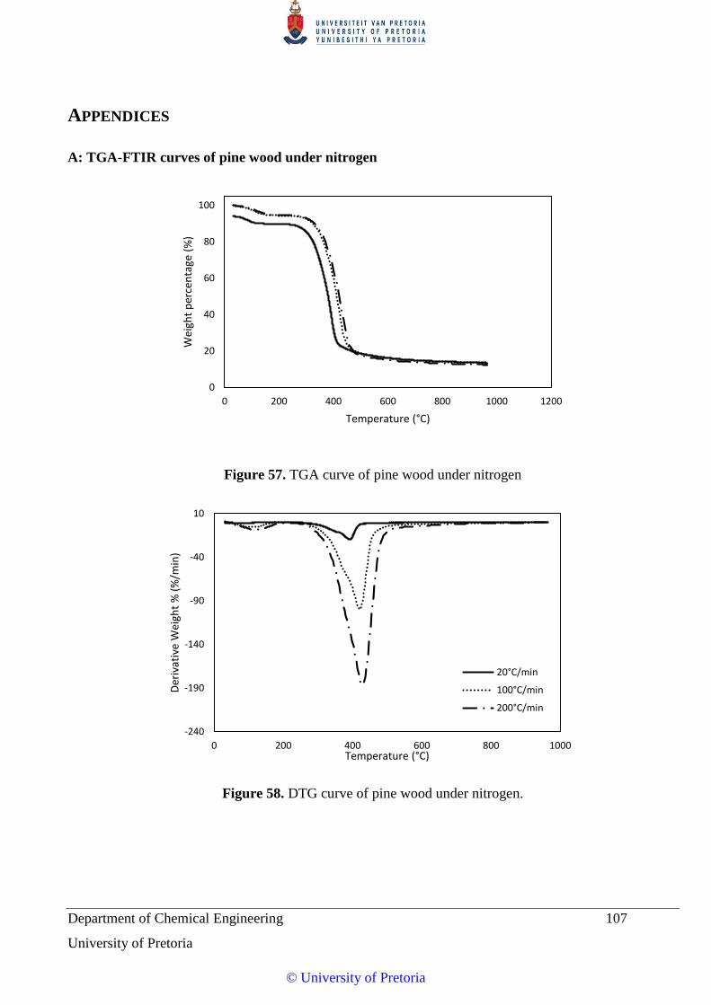
Department of Chemical Engineering 107
University of Pretoria
APPENDICES
A: TGA-FTIR curves of pine wood under nitrogen
Figure 57. TGA curve of pine wood under nitrogen
Figure 58. DTG curve of pine wood under nitrogen.
0
20
40
60
80
100
0 200 400 600 800 1000 1200
Wei
ght
per
cen
tage
(%
)
Temperature (°C)
-240
-190
-140
-90
-40
10
0 200 400 600 800 1000
Der
ivat
ive
Wei
ght
% (
%/m
in)
Temperature (°C)
20°C/min
100°C/min
200°C/min
© University of Pretoria

Makaringe Appendices
Department of Chemical Engineering 108
University of Pretoria
Figure 59. FTIR spectra of pine wood at 100°C/min under nitrogen.
-0.005
0
0.005
0.01
0 1000 2000 3000 4000 5000
Ab
s
Wave number cm-1
83.46 °C
0
0.02
0.04
0.06
0.08
0 1000 2000 3000 4000 5000
Ab
s
Wave number cm-1
108.95 °C
0
0.01
0.02
0.03
0.04
0.05
0.06
0 1000 2000 3000 4000 5000
Ab
s
Wave number cm-1
320.87 °C
0
0.05
0.1
0.15
0.2
0 1000 2000 3000 4000 5000
Ab
s
Wave number cm-1
344.43 °C
0
0.02
0.04
0.06
0.08
0.1
0 1000 2000 3000 4000 5000
Ab
s
Wave number cm-1
390.01 °C
0
0.05
0.1
0.15
0.2
0.25
0.3
0 1000 2000 3000 4000 5000
Ab
s
Wave number cm-1
420.00 °C
© University of Pretoria

Makaringe Appendices
Department of Chemical Engineering 109
University of Pretoria
B: TGA-FTIR curves of Napier grass under nitrogen
Figure 60. TGA curves of Napier grass under nitrogen
Figure 61. DTG curve of Napier grass under nitrogen.
0
20
40
60
80
100
0 200 400 600 800 1000
Wei
ght
per
cen
tatg
e (%
)
Temperature (°C)
20°C/min
100°C/min
200°C/min
-290
-240
-190
-140
-90
-40
10
0 200 400 600 800 1000
Der
ivat
ive
Wei
ght
% (
%/m
in)
Temperature (°C)
20°C/min
100°C/min
200°C/min
© University of Pretoria

Makaringe Appendices
Department of Chemical Engineering 110
University of Pretoria
Figure 62. FTIR spectra of Napier grass at 20°C/min under nitrogen.
-0.006
-0.004
-0.002
0
0.002
0.004
0.006
0.008
0.01
0 1000 2000 3000 4000 5000
Ab
s
Wave number cm-1
86.73 °C
-0.02
0
0.02
0.04
0.06
0.08
0.1
0.12
0 1000 2000 3000 4000 5000A
bs
Wave number cm-1
333.73 °C
© University of Pretoria

Makaringe Appendices
Department of Chemical Engineering 111
University of Pretoria
Figure 63. FTIR spectra of Napier grass at 100°C/min under nitrogen.
0
0.01
0.02
0.03
0.04
0.05
0 1000 2000 3000 4000 5000
Ab
s
Wave number cm-1
112.38 °C
0
0.1
0.2
0.3
0.4
0.5
0.6
0 1000 2000 3000 4000 5000
Ab
s
Wave number cm-1
357.63 °C
© University of Pretoria

Makaringe Appendices
Department of Chemical Engineering 112
University of Pretoria
C: TGA-FTIR curves of peach pips under nitrogen
Figure 64. TGA curves of peach pips under nitrogen
Figure 65. DTG curve of peach pips under nitrogen.
0
20
40
60
80
100
0 200 400 600 800 1000
Wei
ght
per
cen
tage
(%
)
Temperature (°C)
20°C/min
100°C/min
200°C/min
-150
-130
-110
-90
-70
-50
-30
-10
10
0 200 400 600 800 1000
Der
ivat
ive
Wei
ght
% (
%/m
in)
Temperature (°C)
20°C/min100°C/min200°C/min
© University of Pretoria

Makaringe Appendices
Department of Chemical Engineering 113
University of Pretoria
Figure 66. FTIR spectra of peach pips at 20°C/min under nitrogen.
-0.005
0
0.005
0.01
0.015
0.02
0.025
0 1000 2000 3000 4000 5000
Ab
s
Wave numbe cm-1
88.43 °C
-0.01
0
0.01
0.02
0.03
0.04
0.05
0.06
0.07
0.08
0.09
0 1000 2000 3000 4000 5000A
bs
Wave number cm-1
307.47 °C
0
0.01
0.02
0.03
0.04
0.05
0.06
0 1000 2000 3000 4000 5000
Ab
s
Wave number cm-1
373.55 °C
© University of Pretoria

Makaringe Appendices
Department of Chemical Engineering 114
University of Pretoria
Figure 67. FTIR spectra of peach pips at 100°C/min under nitrogen.
0
0.005
0.01
0.015
0.02
0.025
0.03
0.035
0.04
0 1000 2000 3000 4000 5000
Ab
s
Wave number cm-1
121.38 °C
0
0.05
0.1
0.15
0.2
0.25
0.3
0 1000 2000 3000 4000 5000A
bs
Wave number cm-1
342.69 °C
0
0.05
0.1
0.15
0.2
0.25
0 1000 2000 3000 4000 5000
Ab
s
Wave number cm-1
279.4 °C
© University of Pretoria
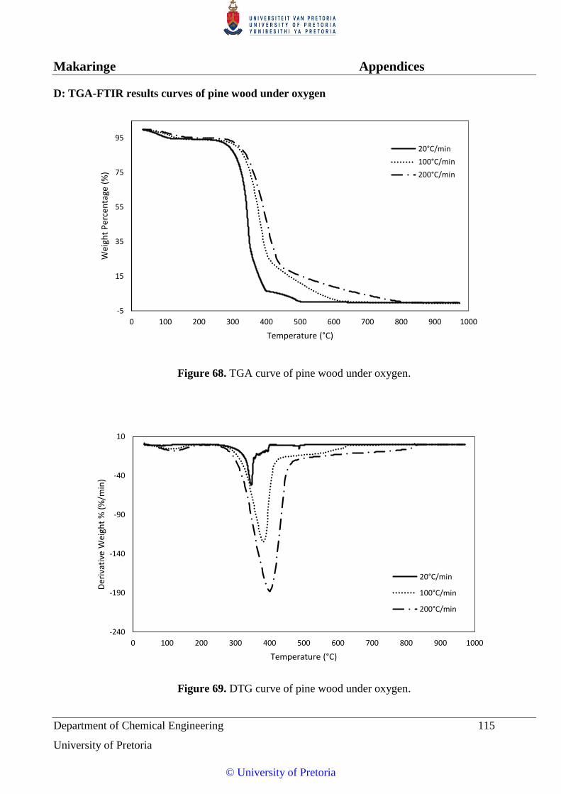
Makaringe Appendices
Department of Chemical Engineering 115
University of Pretoria
D: TGA-FTIR results curves of pine wood under oxygen
Figure 68. TGA curve of pine wood under oxygen.
Figure 69. DTG curve of pine wood under oxygen.
-5
15
35
55
75
95
0 100 200 300 400 500 600 700 800 900 1000
Wei
ght
Per
cen
tage
(%
)
Temperature (°C)
20°C/min
100°C/min
200°C/min
-240
-190
-140
-90
-40
10
0 100 200 300 400 500 600 700 800 900 1000
Der
ivat
ive
Wei
ght
% (
%/m
in)
Temperature (°C)
20°C/min
100°C/min
200°C/min
© University of Pretoria

Makaringe Appendices
Department of Chemical Engineering 116
University of Pretoria
Figure 70. FTIR spectra of pine wood at 20°C/min under oxygen.
0
0.1
0.2
0.3
0.4
0.5
0 1000 2000 3000 4000 5000
Ab
s
Wave number cm-1
80.64 °C
0
0.1
0.2
0.3
0.4
0.5
0.6
0 1000 2000 3000 4000 5000
Ab
s
Wave number cm-1
347.50 °C
0
0.05
0.1
0.15
0.2
0.25
0.3
0 500 1000 1500 2000 2500 3000 3500 4000 4500
Ab
s
Wave number cm-1
486.22 °C
© University of Pretoria

Makaringe Appendices
Department of Chemical Engineering 117
University of Pretoria
Figure 71. FTIR spectra of pine wood at 100°C/min under oxygen.
0
0.005
0.01
0.015
0.02
0.025
0.03
0.035
0.04
0.045
0.05
0 1000 2000 3000 4000 5000
Ab
s
Wave number cm-1
107.84 °C
0
0.1
0.2
0.3
0.4
0.5
0.6
0.7
0.8
0 1000 2000 3000 4000 5000A
bs
Wave number cm-1
381.14 °C
0
0.1
0.2
0.3
0.4
0.5
0.6
0.7
0.8
0 500 1000 1500 2000 2500 3000 3500 4000 4500
Ab
s
Wave number cm-1
566.01 °C
© University of Pretoria
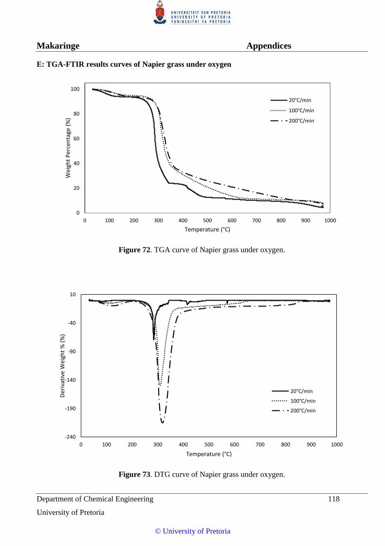
Makaringe Appendices
Department of Chemical Engineering 118
University of Pretoria
E: TGA-FTIR results curves of Napier grass under oxygen
Figure 72. TGA curve of Napier grass under oxygen.
Figure 73. DTG curve of Napier grass under oxygen.
0
20
40
60
80
100
0 100 200 300 400 500 600 700 800 900 1000
Wei
ght
Per
cen
tage
(%
)
Temperature (°C)
20°C/min
100°C/min
200°C/min
-240
-190
-140
-90
-40
10
0 100 200 300 400 500 600 700 800 900 1000
Der
ivat
ive
Wei
ght
% (
%)
Temperature (°C)
20°C/min
100°C/min
200°C/min
© University of Pretoria

Makaringe Appendices
Department of Chemical Engineering 119
University of Pretoria
Figure 74. FTIR spectra of Napier grass at 20°C/min under oxygen.
0
0.02
0.04
0.06
0.08
0.1
0.12
0.14
0.16
0 1000 2000 3000 4000 5000
Ab
s
Wave number cm-1
83.21 °C
0
0.1
0.2
0.3
0.4
0.5
0.6
0.7
0 1000 2000 3000 4000 5000A
bs
Wave number cm-1
284.16 °C
0
0.05
0.1
0.15
0.2
0.25
0.3
0.35
0 1000 2000 3000 4000 5000
Ab
s
Wave number cm-1
571.46 °C
© University of Pretoria

Makaringe Appendices
Department of Chemical Engineering 120
University of Pretoria
Figure 75. FTIR spectra of Napier grass at 100°C/min under oxygen.
-0.005
0
0.005
0.01
0.015
0.02
0 1000 2000 3000 4000 5000
Ab
s
Wave number cm-1
122.69 °C
0
0.1
0.2
0.3
0.4
0.5
0.6
0.7
0.8
0.9
0 500 1000 1500 2000 2500 3000 3500 4000 4500
Ab
s
Wave number cm-1
319.77 °C
© University of Pretoria

Makaringe Appendices
Department of Chemical Engineering 121
University of Pretoria
Figure 76. FTIR spectra of Napier grass at 200°C/min under oxygen.
-0.02
-0.015
-0.01
-0.005
0
0.005
0.01
0.015
0.02
0.025
0 1000 2000 3000 4000 5000
Ab
s
Wave number cm-1
122.69 °C
-0.01
0.09
0.19
0.29
0.39
0.49
0.59
0.69
0.79
0.89
0 1000 2000 3000 4000 5000
Ab
s
Wave number cm-1
319.77 °C
© University of Pretoria
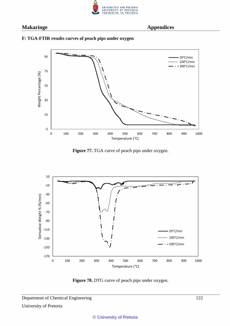
Makaringe Appendices
Department of Chemical Engineering 122
University of Pretoria
F: TGA-FTIR results curves of peach pips under oxygen
Figure 77. TGA curve of peach pips under oxygen.
Figure 78. DTG curve of peach pips under oxygen.
-5
15
35
55
75
95
0 100 200 300 400 500 600 700 800 900 1000
Wei
ght
Per
cen
tage
(%
)
Temperature (°C)
20°C/min
100°C/min
200°C/min
-170
-150
-130
-110
-90
-70
-50
-30
-10
10
0 100 200 300 400 500 600 700 800 900 1000
Der
ivat
ive
Wei
ght
% (
%/m
in)
Temperature (°C)
20°C/min
100°C/min
200°C/min
© University of Pretoria

Makaringe Appendices
Department of Chemical Engineering 123
University of Pretoria
Figure 79. FTIR spectra of peach pips at 20°C/min under oxygen.
-0.01
0.01
0.03
0.05
0.07
0.09
0.11
0.13
0 1000 2000 3000 4000 5000
Ab
s
Wave number cm-1
90.10 °C
0
0.05
0.1
0.15
0.2
0.25
0 1000 2000 3000 4000 5000
Ab
sWave number cm-1
303.80 °C
-0.01
0.04
0.09
0.14
0.19
0.24
0.29
0.34
0.39
0.44
0 1000 2000 3000 4000 5000
Ab
s
Wave number cm-1
324.83 °C
© University of Pretoria

Makaringe Appendices
Department of Chemical Engineering 124
University of Pretoria
Figure 80. FTIR spectra of peach pips at 100°C/min under oxygen.
-0.02
-0.01
0
0.01
0.02
0.03
0.04
0.05
0.06
0 1000 2000 3000 4000 5000
Ab
s
Wave number cm-1
116.81 °C
0
0.05
0.1
0.15
0.2
0.25
0.3
0.35
0.4
0.45
0 1000 2000 3000 4000 5000A
bs
Wave number cm-1
333.74 °C
0
0.1
0.2
0.3
0.4
0.5
0.6
0 1000 2000 3000 4000 5000
Ab
s
Wave number cm-1
373.17 °C
© University of Pretoria

Makaringe Appendices
Department of Chemical Engineering 125
University of Pretoria
Figure 81. FTIR spectra of peach pips at 200°C/min under oxygen.
0
0.005
0.01
0.015
0.02
0.025
0.03
0 1000 2000 3000 4000 5000
Ab
s
Wave number cm-1
136.20 °C
0
0.05
0.1
0.15
0.2
0.25
0 1000 2000 3000 4000 5000
Ab
sWave number cm-1
351.18 °C
0
0.1
0.2
0.3
0.4
0.5
0.6
0.7
0.8
0.9
1
0 1000 2000 3000 4000 5000
Ab
s
Wave number cm-1
388.49 °C
© University of Pretoria


