PLASTIC YIELDING CHARACTERISTICS OF A ROD UNDER SUCCESSIVELY APPLIED TORSION AND TENSION LOADINGS. / i ABU RAYHAN MOHAMMAD ALI, M Sc Eng. This thesis is submitted to Dublin City University as the fulfilment of the requirement for the award of Degiee of Doctor of Philosophy School of Mechanical and Manufacturing Engineering Dublin City University June 1995 i
Transcript
PLASTIC YIELDING CHARACTERISTICS OF A ROD UNDER SUCCESSIVELY APPLIED TORSION AND
TENSION LOADINGS.
/
i
ABU RAYHAN MOHAMMAD ALI, M Sc Eng.
This thesis is submitted to Dublin City University as the fulfilment of the requirementfor the award of Degiee of
Doctor o f Philosophy
School o f Mechanical and Manufacturing Engineering Dublin City University
June 1995
i
Dedicated to my parents
DECLARATION
This is to certify that the material presented in this thesis is entuely my own work, except
where specific references have been made to the works of others, and no part of this work has
been submitted in support of an application for another degree or qualification to this or any
other establishment
Signed ID 91700566
Abu Rayhan Mohammad Ah
June 1995
I
ACKNOW LEDGEM ENTS
I would like to thank to Professor M S J Hashmi for his supervision and guidance dunng
this research work Thanks are also expressed to Dr M El-Baradie for his helpful suggestions
from time to time dunng my studies
I would also like to thank to Piofessor S A Meguid of the University of Toronto for his
constructive suggestions and helpful advice during his short visit to DCU I highly appreciate
the help of Dr L Looney for her comments on the initial draft of the thesis
I would like to expiess my thanks to Mr Liam Doimican and Mr Ian Hopper for their
technical assistance at various stages of this woik
Finally, the patience and encouragement of my wife, Sharmin, and family deserve greater
acknowledgement than words can express
II
ABSTRACT
Plastic yielding characteristics of a rod under successively
applied torsion and tension loadings
By
Abu Rayhan Mohammad All
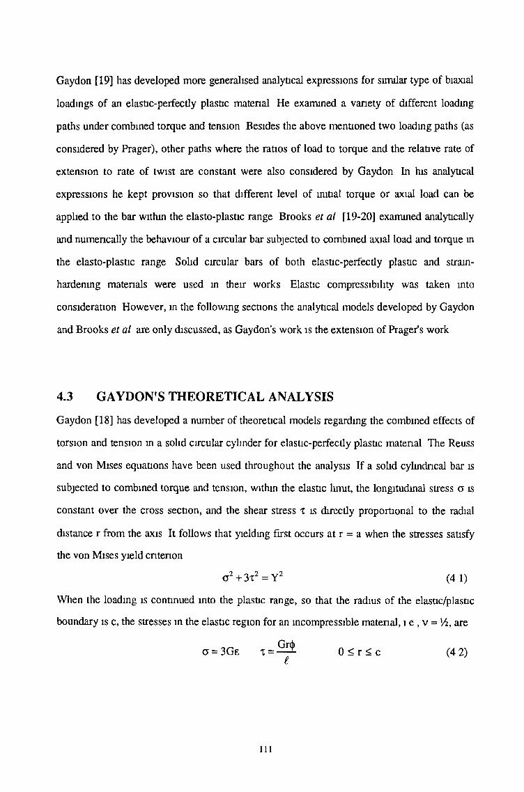
This thesis is concerned with the elasto-plastic behaviour of circular rods under combined torsion-tension loading Three aspects of the work were examined In the first, an instrumented mechanical torque-tension machine was designed, built and commissioned to enable the application of biaxial loading under controlled conditions The main features of the machine are (1) it can apply either simultaneous or individual loadings subject to a specific deformation history and (11) it provides the time variations of the controlling and the controlled deformation parameters using the appropriate load cells and tranducing elements Whilst the machine was controlled by analogue signals, it was designed such that it could allow digital control of the different command signals An analytical model to calculate the stiffness of the machine has been developed
The second was wholly devoted to the experimental investigations where solid, copper and steel, circular rods were subjected to complex non-proportional biaxial loading paths In these paths, elasto-plastic torsion followed by tension, keeping the angle of twist constant, and elasto-plastic tension followed by torsion, holding the corresponding axial displacement constant, were examined Other loading paths, where the initial axial loads and the torques were maintained constant, and where the torque and the axial load were applied successively, were also studied The expenmental programme also considered the biaxial loading of thin- walled steel tubes In the third, the experimental results were compared with two different analytical models from the literature Numerical solutions were also obtained along the lines descnbed in an available literature
Expenmentally, it has been observed that when the rod is initially subjected to a torque and then, keeping the angle of twist constant, to a gradually increasing axial load, the rod behaves as if its torque carrying ability becomes drastically reduced without in any way affecting its load carrying ability Similarly, when the rod is initially subjected to an axial load and then, keeping the axial displacement constant, to a gradually increasing torque, the rod behaves as if its load carrying ability becomes drastically reduced without in any way affecting its torque
III
carrying ability Such reductions in the load or torque capacity appear to be governed by the material plastic yield criterion
During the successively applied loading, it has been observed that when the rod is initially subjected to an initial torque and then to a successively applied axial load and torque, keeping the axial displacement or the angle of twist constant in an alternate manner, the rod soon regains its axial load carrying capability irrespective of the initially applied torque Similarly, during the multiple alterations of successively applied torque or axial load, it has been observed that at any stage for the axial load or torque, whichever was applied subsequently, the rod regains its carrying capability of the parameter involved Experimental test results with fitted strain gauges show that, even when the angle of twist or axial displacement was held constant, the strain readings increase rapidly with the decrease of the initially applied torque or axial load at the confined zone where the plastic deformation begins Elsewhere of the specimen the strain readings decrease
The findings of this work have direct bearing on the relaxation of tightening torques or axial loads as experienced by critical engineering components, such as couplings, bolted joints and rotating shafts, which are subjected to similar type of biaxial loadings
IV
NOMENCLATURE
A cross-sectional areaA0, B0 funtion defined in equation 4 36(a)
E Young's modulusF axial loadF normalised axial load (F/Fy)G modulus of rigidityH' slope of effective stress generalized plastic strain curveI second moment of inertiaJ polar moment of inertiaJj first invariant of strain
L lengthP ratio of shear stress to yield shearQ ratio of axial stress to uniaxial yield stressT torqueT normalised torque (T/Ty)Y yield stress in tensiona radius of solid rodc radius of the elastic-plastic boundaryk yield stress in shearI lengthn strain hardening parametern safety factor in designingu, v, w displacementskf stress concentration factor
R outer radius of solid rodr r/Ra a constant
8 Kronecker delta
v Poisson's ratio0/<j> angle of twistp parameter characterizing state of plastic deformationG axial stress
V
Gy general stress tensor
Gy deviator stress tensor
G effective stressGm dimensionless volumetric stress
a dimensionless effective stress
a r, a 0, a z, Ga, x dimensionless stresses
Gr,G0,a z,x dimensionless deviatone stresses
x shear stresse axial straine nonnalised axial strain ( e /£ y )
7 shear strain
y nonnalised shear strain (7/7y)
£r,e0,£z,ea modified strains
£y general strain tensor
£p generalized plastic strain
£p modified generalized plastic strain
er, eô, ez, y deviator strains
er , e0, ez modified deviatone strain
X propotionahty factor in Lévy - Mises equationr| = c/a
subscriptsa alternating component of the stresse elastic componentm volumetnc componento any arbitrary loading conditionp plastic component
VI
y yield conditionx,y,z,xy,yz,zx refered to cartesian co-oidinatesr,0,r0,0z,zr refered to cartesian co-ordinates
1,2,3 principal componentsme mean components of the stressen endurance limit
#
VII
LIST OF FIGURES
Chapter One Page no,Figure -1.1 - The method of approach adopted in the present study 10
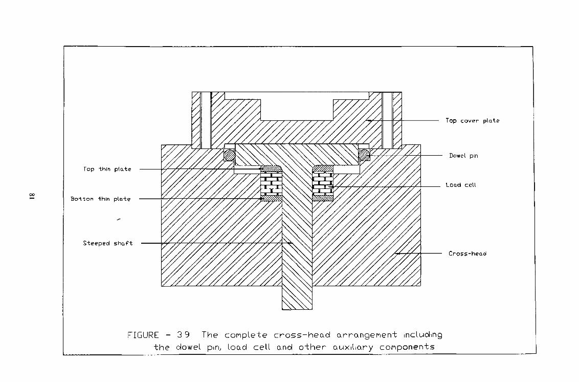
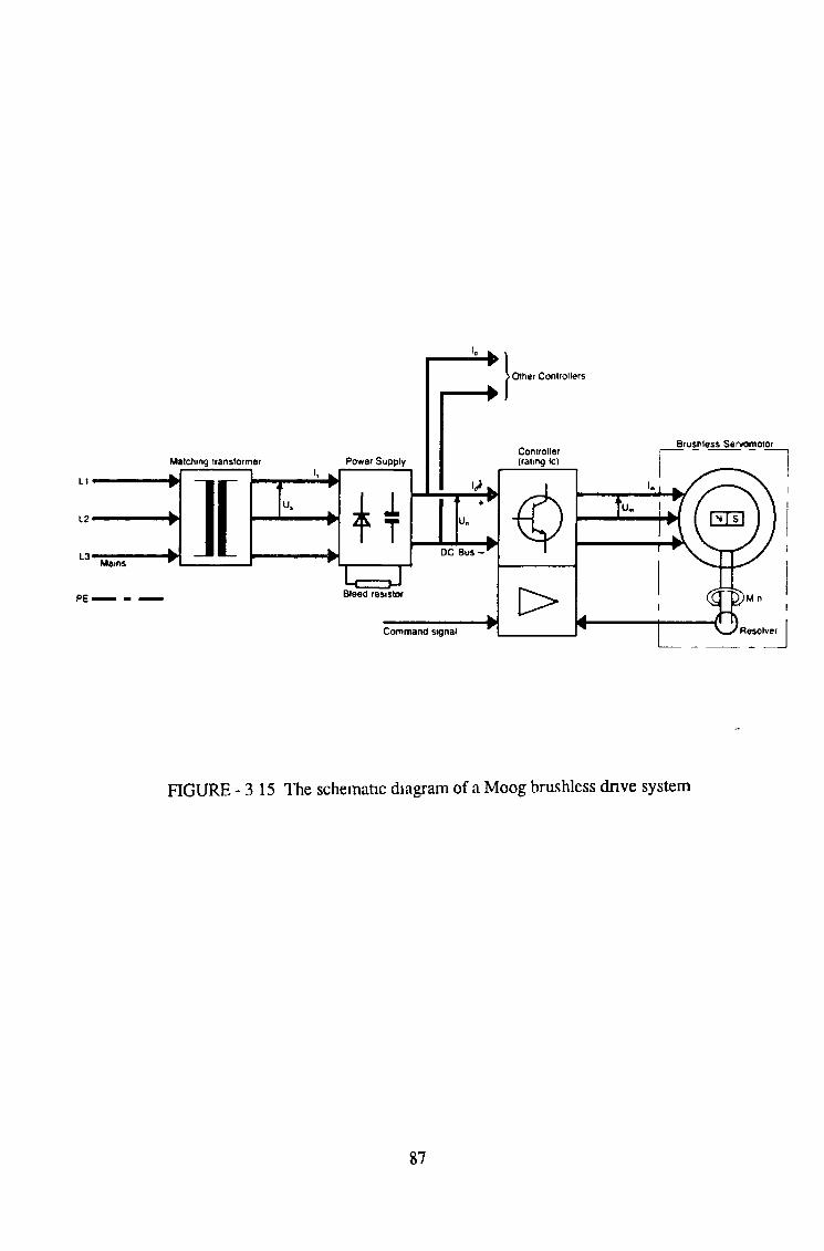
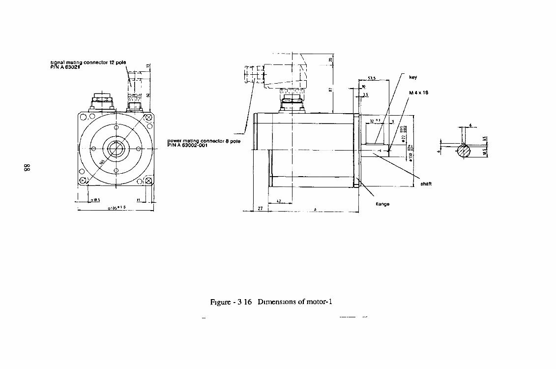
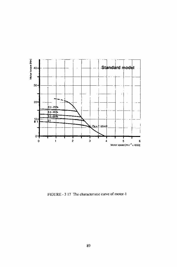
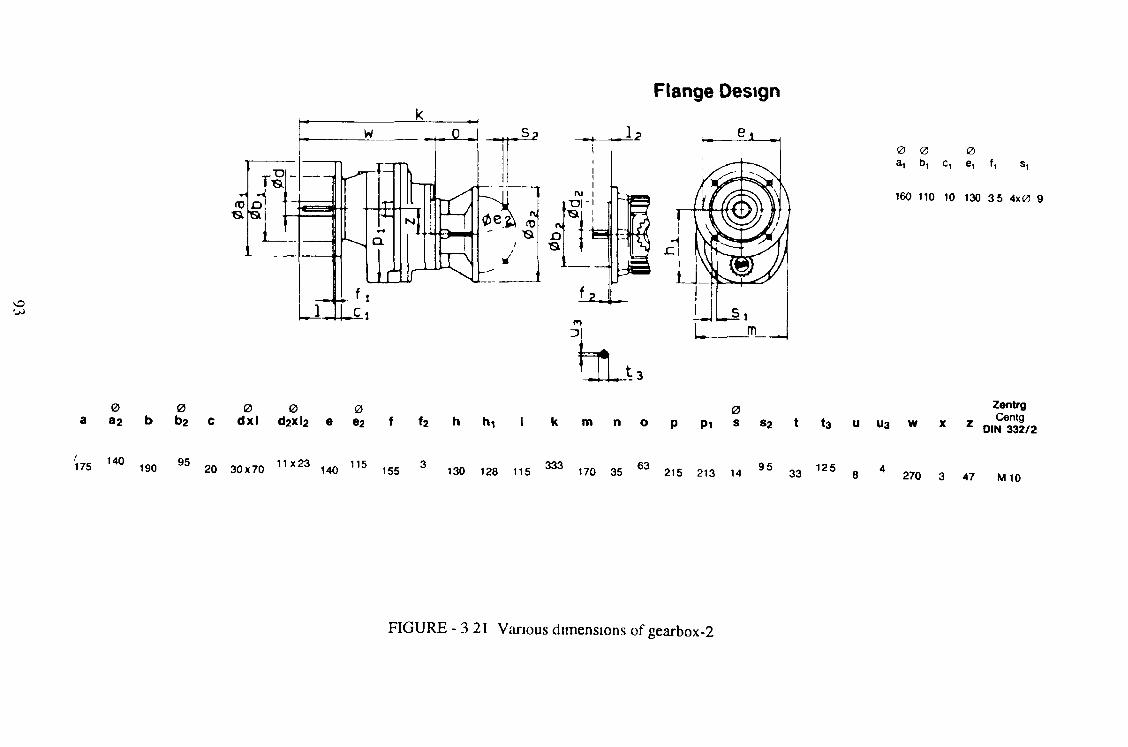
Chapter ThreeFigure - 3.1 - Schematic diagram of the machine (front view) 73Figure - 3.2 - Schematic diagram of the machine (side view) 74Figure - 3.3 - Schematic diagram of the main frame of the machine 75Figure - 3.4 - Details of the bottom plate 76Figure - 3.5 - Details of the drive shaft housing 77Figure - 3.6 - Details of the top plate 78Figure - 3.7 - Details of the ball screw 79Figure - 3.8 - Details of the cross-head 80Figure - 3.9 - The complete cross-head arrangement including the dowel pin
load cell and other auxiliary components81
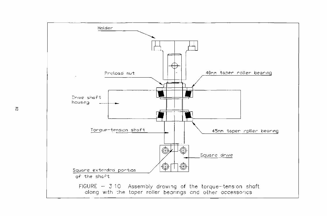
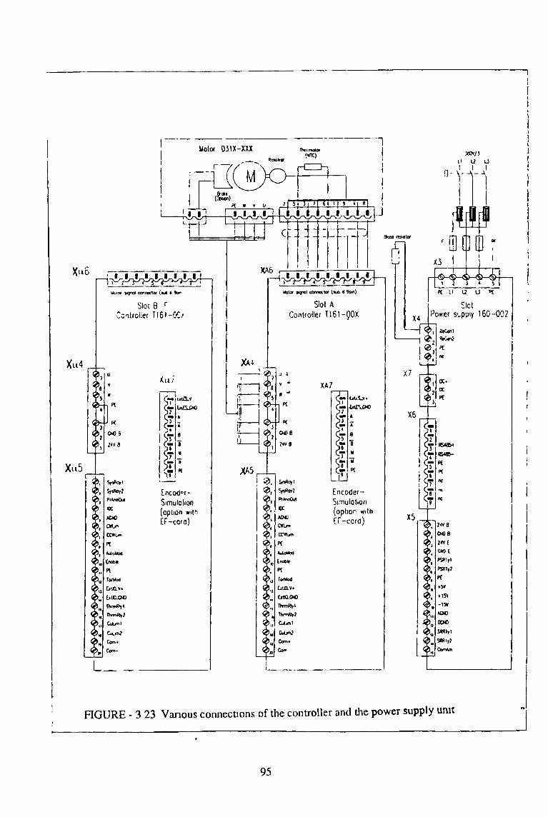
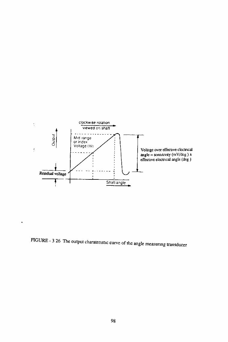
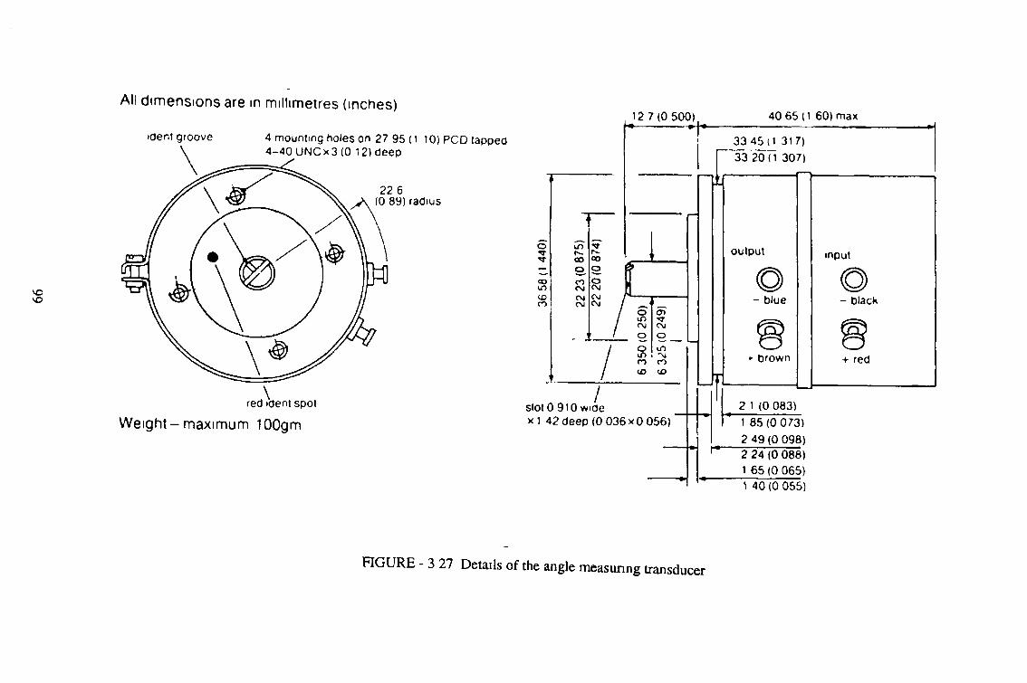
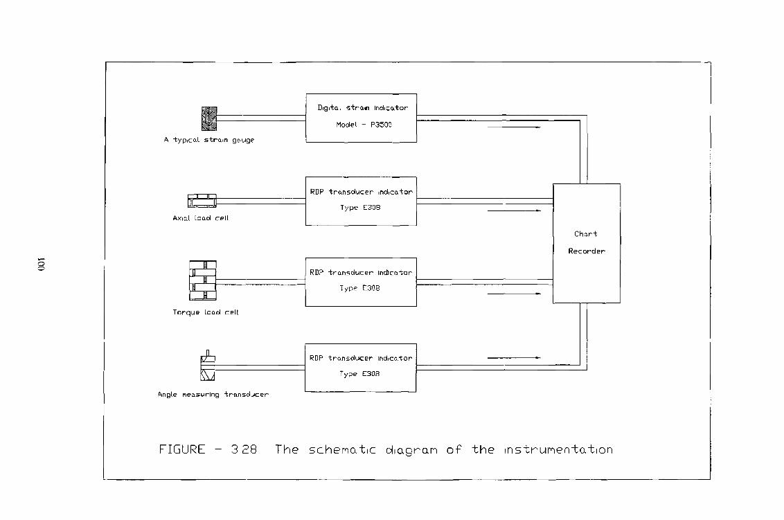
Figure - 3.10 - Assembly drawing of the torque-tension shaft 82Figure - 3.11 - Assembly drawing of the torsion shaft 83Figure - 3.12 - Geometry of the specimen holder 84Figure - 3.13 - Dimension of the gripper in detailed 85Figure - 3.14 - Assembly drawing of the preloading unit 86Figure - 3.15 - Schematic diagram of a Moog brushless drive system 87Figure - 3.16 - Dimensions of motor-1 88Figure - 3.17 - The characteristic curve of motor-1 89Figure - 3.18 - Details of gearbox-1 90Figure - 3.19 - Details of motor-2 91Figure - 3.20 - The characteristic curve of motor-2 92Figure - 3.21 - Various dimension of gearbox-2 93Figure - 3.22 - The flow chart of the operating principle of the controllers 94Figure - 3.23 - Various connections of the controller and the power supply unit 95Figure - 3.24 - Circuit diagram among the controllers and motors 96Figure - 3.25 - The schematic diagram of the control panel 97Figure - 3.26 - The output characteristic curve of the angle measuring transducer 98Figure - 3.27 - Details of the angle measuring transducer 99Figure - 3.28 - The schematic diagram of the instrumentation 100Figure - 3.29 - Force analysis diagram of the torque-tension machine (upper part) 101Figure - 3.30 - Force analysis diagram of the torque-tension machine (lower part) 102
VIII
Chapter Four
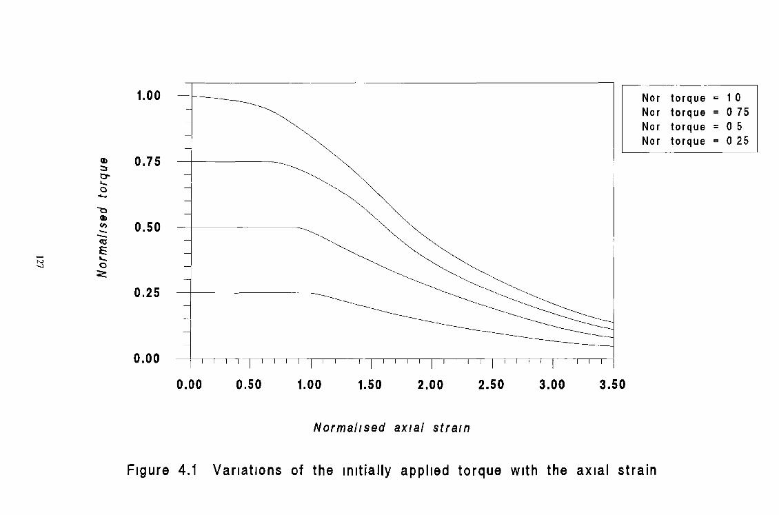
Figure -4 1 - Variations of the initially applied torque with the axial strain 127Figure - 4 2 - Variations of the initially applied axial load with the shear strain 128Figure - 4 3 - Variations of the initially applied torque for different strain 129
hardening parametersFigure - 4 4 - Variations of the initially applied axial load for different strain 130
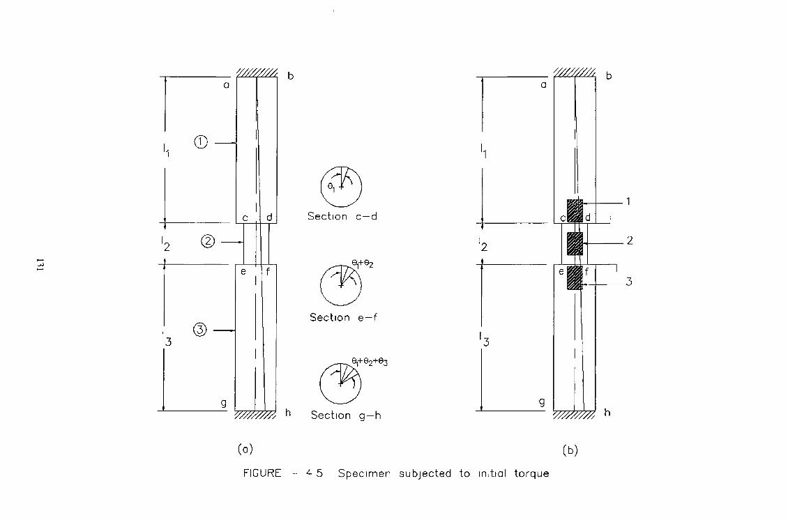
hardening parametersFigure - 4 5 - Specimen subjected to a initial torque 131
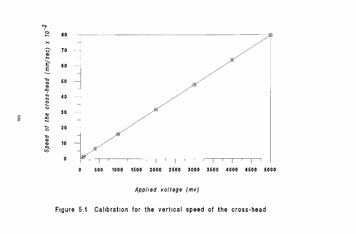
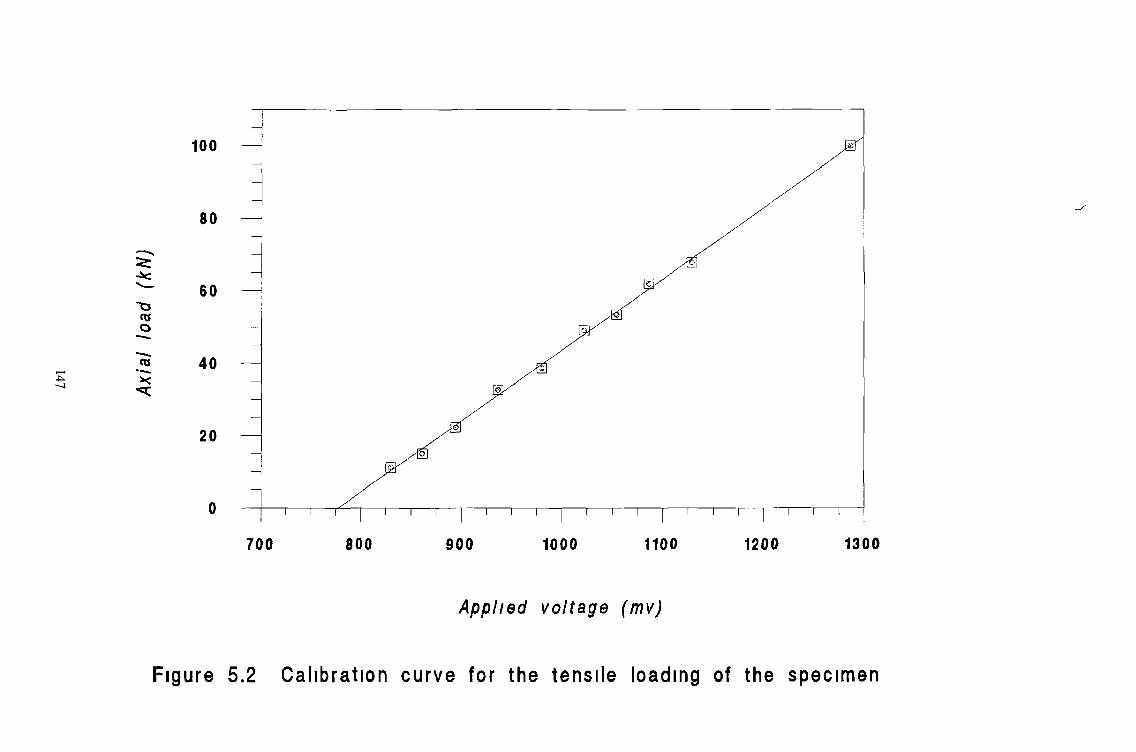
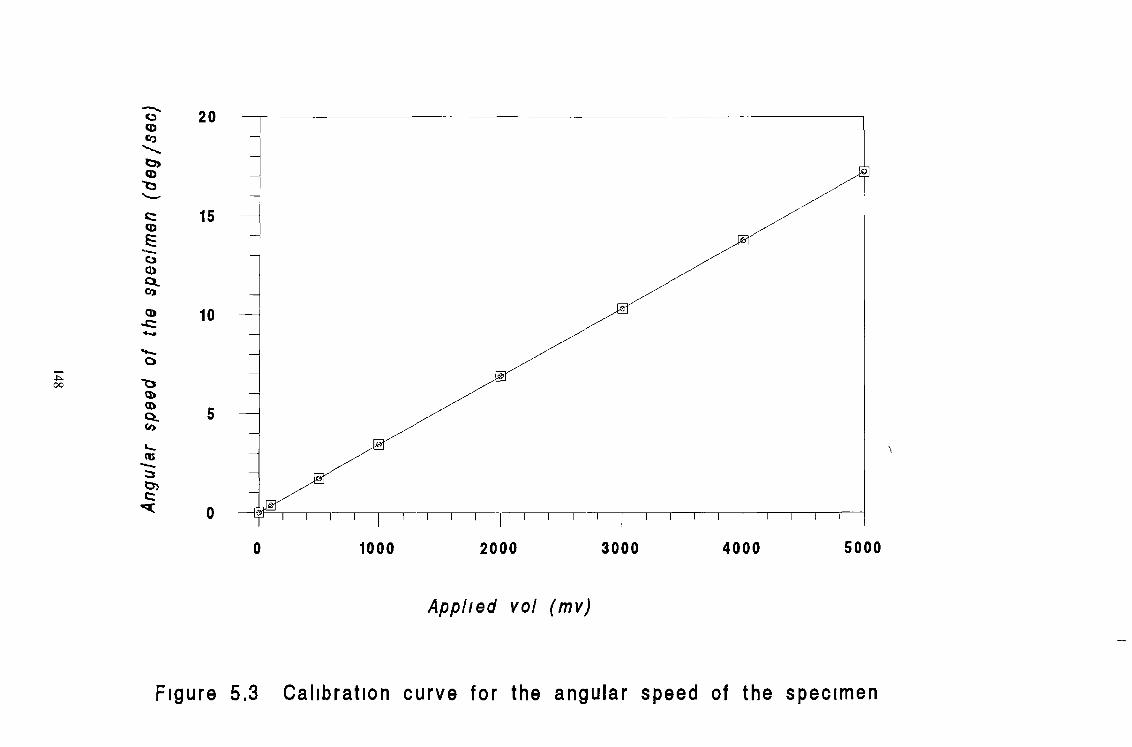
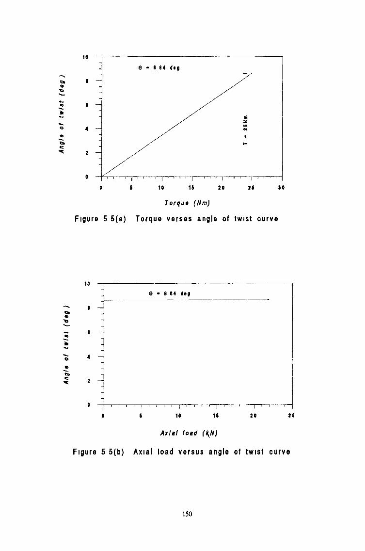
Chapter FiveFigure - 5 1 - Calibration curve for the vertical speed of the cross-head 146Figure - 5 2 - Calibration curve for the tensile loading of the specimen 147Figure - 5 3 - Calibration curve for the angular speed of the specimen 148Figure - 5 4 - Calibration curve for the torque applied to the specimen 149Figure - 5 5(a) - Toique versus angle of twist curve 150Figure - 5 5(b) - Axial load versus angle of twist curve 150Figure - 5 5(c) - Toique versus angle of twist curve when toique maintained 151
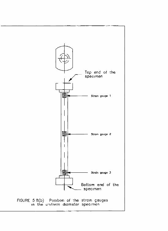
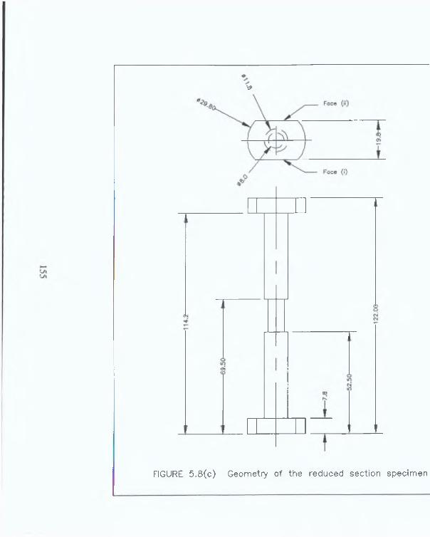
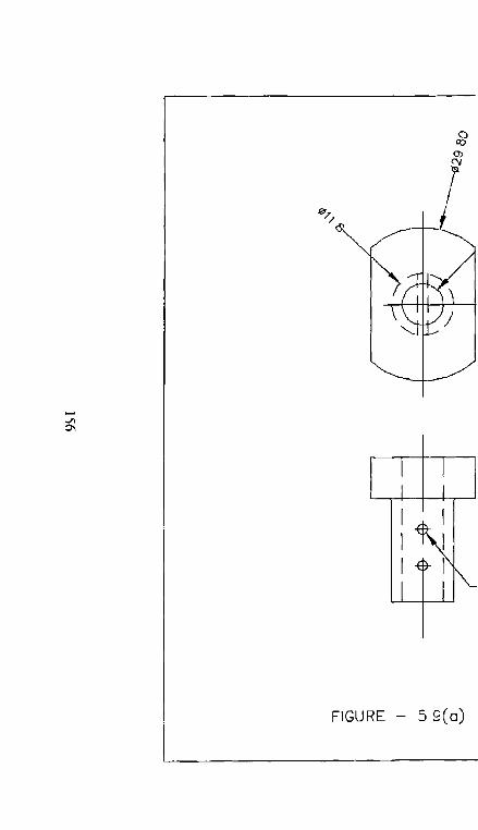
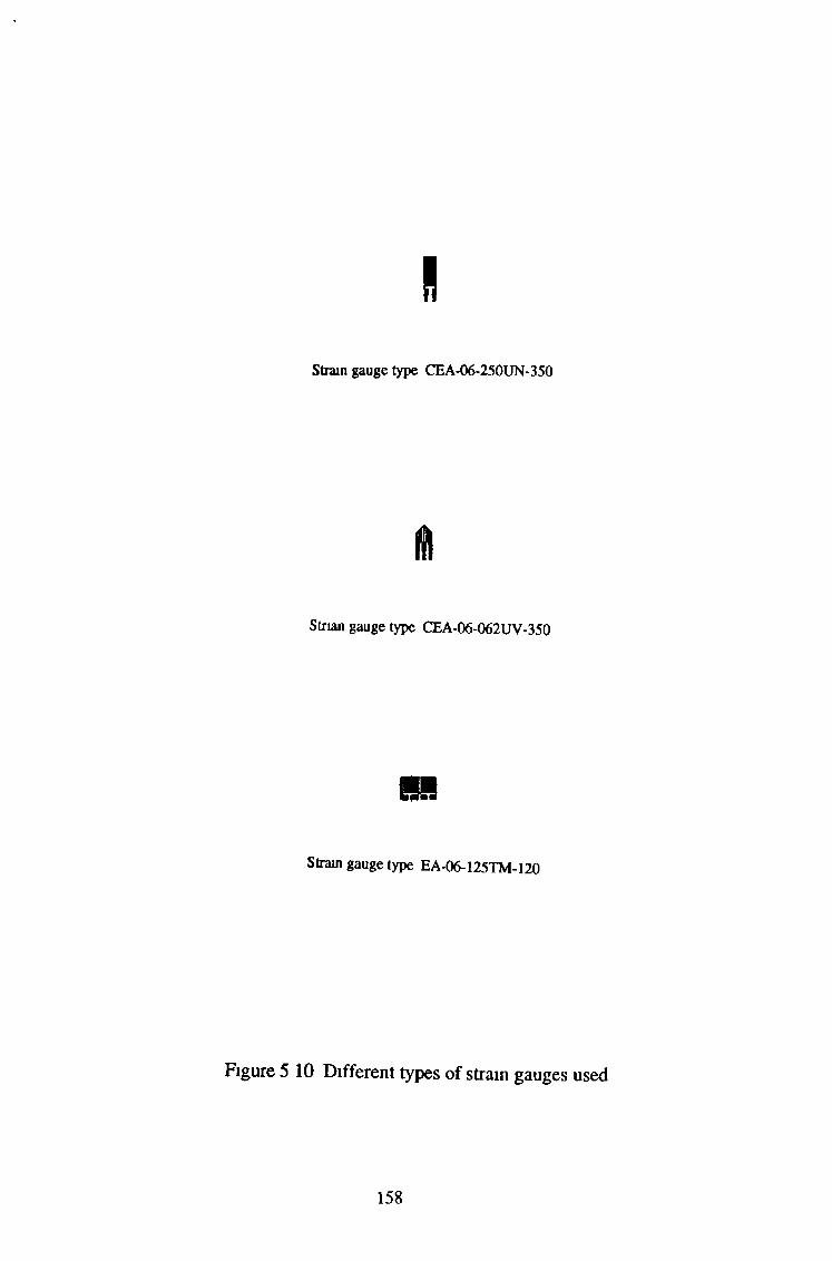
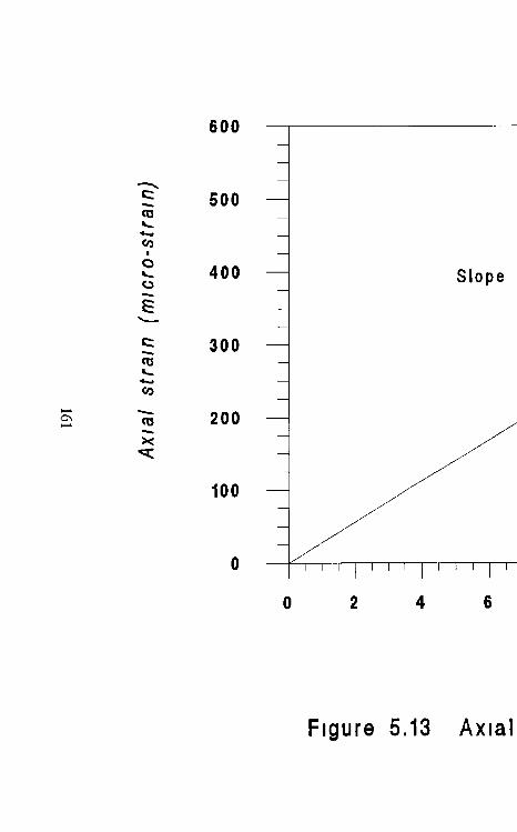
constantFigure - 5 6(a) - Axial load versus axial displacement curve 151Figure - 5 6(b) - Torque versus axial displacement curve 152Figure - 5 6(c) - Torque versus axial load curve when load maintained constant 152Figure - 5 7 - Geometry of the specimen 153Figure - 5 8(a) - Geometry of the uniform diameter specimen 154Figure - 5 8(b) - Position of the strain gauges in the uniform diameter specimen 154Figure - 5 8(c) - Geometry of the reduced section specimen 155Figure - 5 8(d) - Position of the strain gauges in the reduced section specimen 155Figure - 5 9(a) - Specially designed head to fit with the thin-walled tube 156Figure - 5 9(b) - The assembly drawing of the thin- walled tube 157Figure - 5 10 - Different types of strain gauges used 158Figure - 5 11 - Different stages of strain gauges preparation 159Figure - 5 12(a) - A typical full bridge connection between the strain gauges and the 160
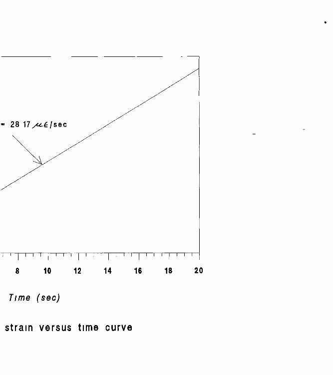
switch and balance unitFigure - 5 12(b) - Circuit diagram between the strain indicator and the balance unit 160Figure - 5 13 - Axial strain versus time curve 161Figure - 5 14 - Shear strain versus time curve 162
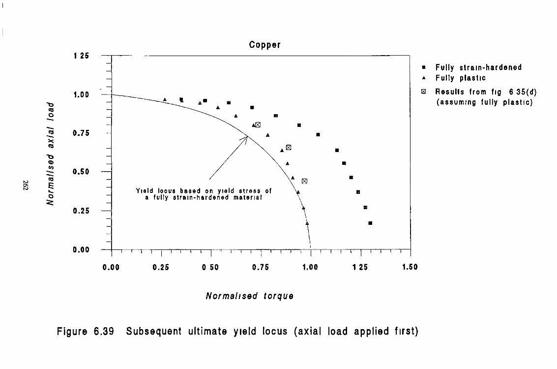
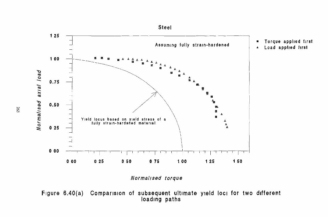
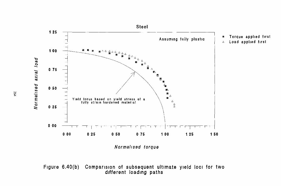
- Subsequent ultimate yield locus for steel (torque applied first)- Subsequent ultimate yield locus for copper (torque applied first)- Subsequent ultimate yield locus for steel (load applied first)- Subsequent ultimate yield locus for copper (load applied first)- Compansion of subsequent ultimate yield loci for two different loading paths (assuming fully strain-hardened)(steel)
- Compansion of subsequent ultimate yield loci for two different loading paths (assuming fully plastic torque)(steel)
- Compansion of subsequent ultimate yield loci for two different loading paths (assuming fully strain-hardened)(copper)
- Compansion of subsequent ultimate yield loci for two different loading paths (assuming fully plastic torque)(copper)
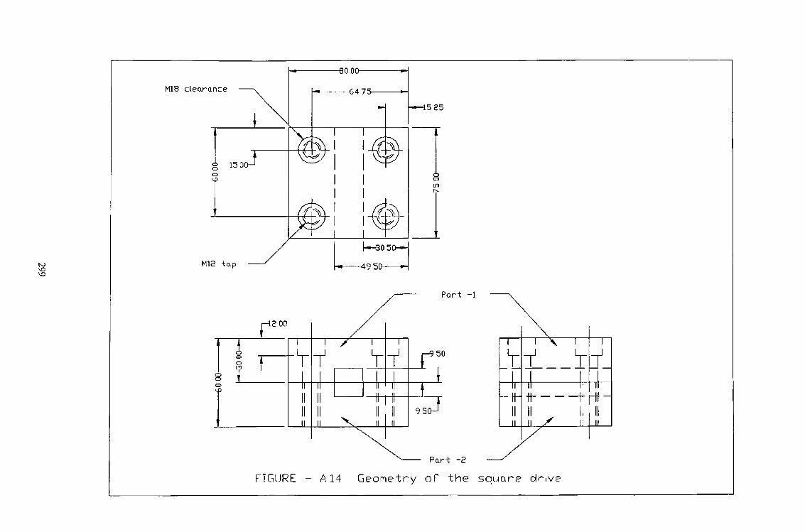
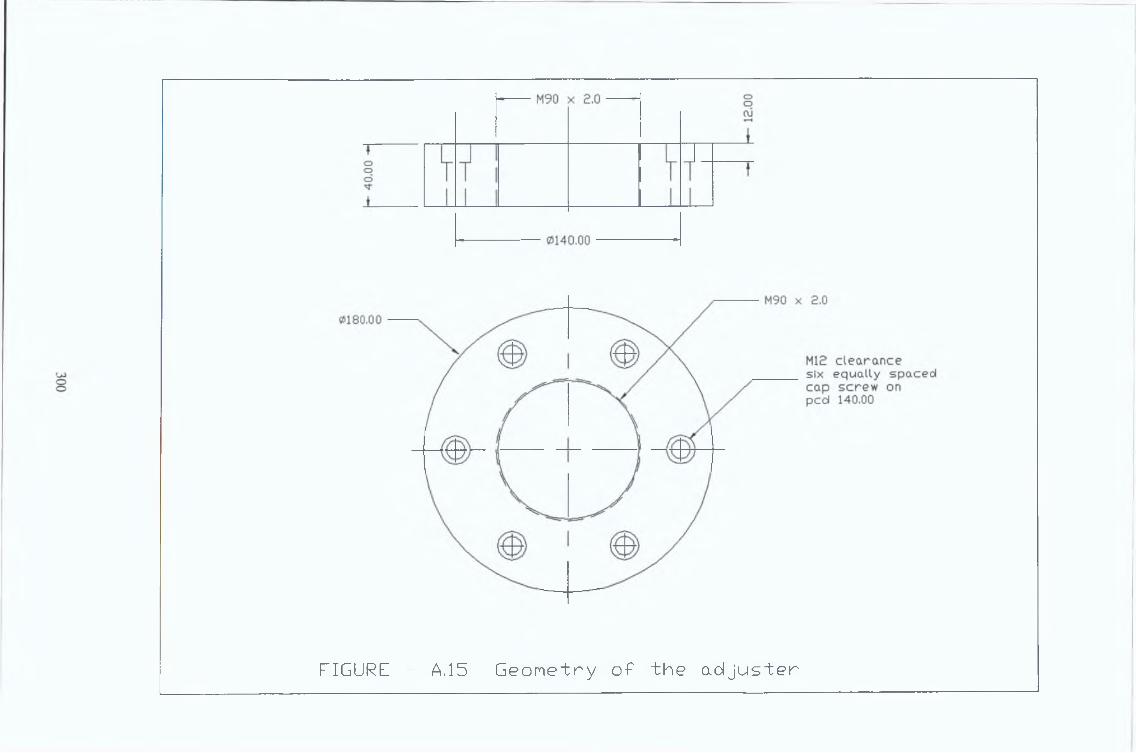
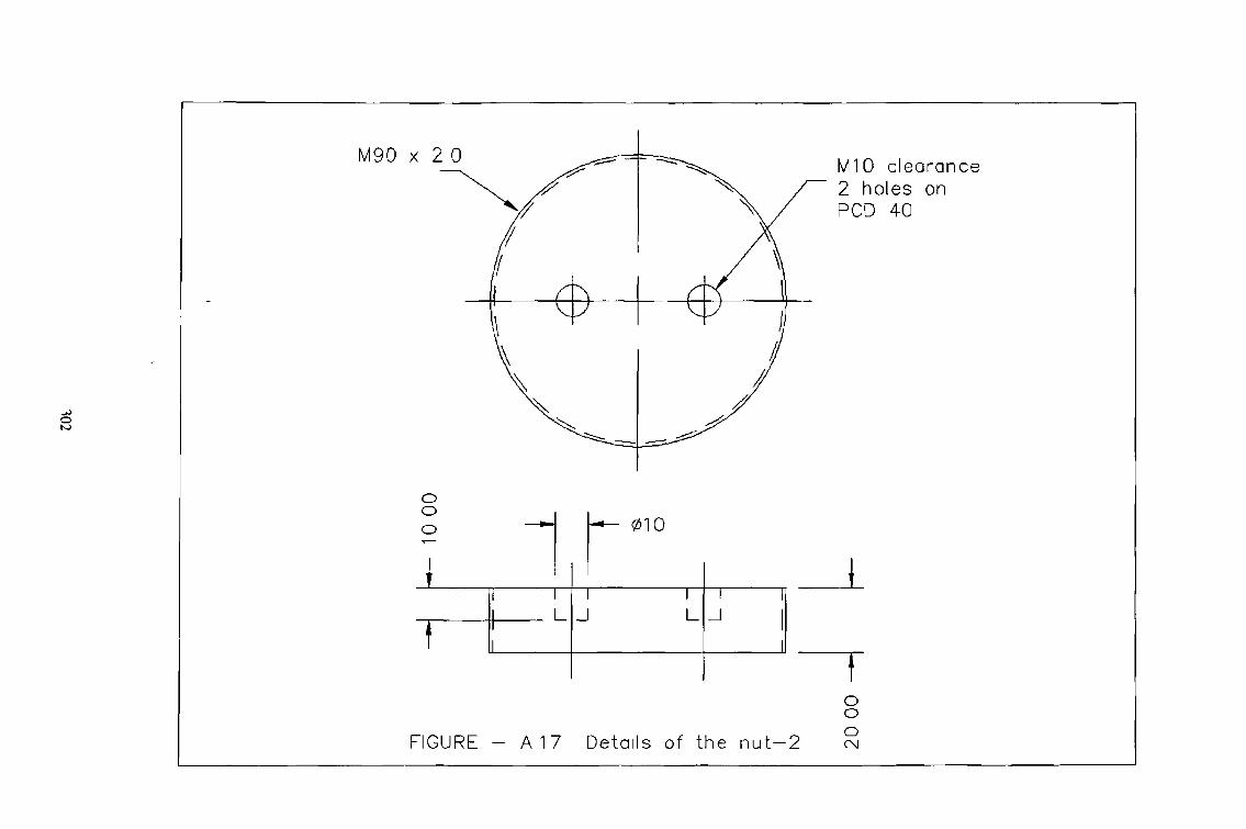
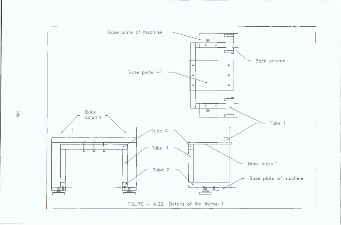
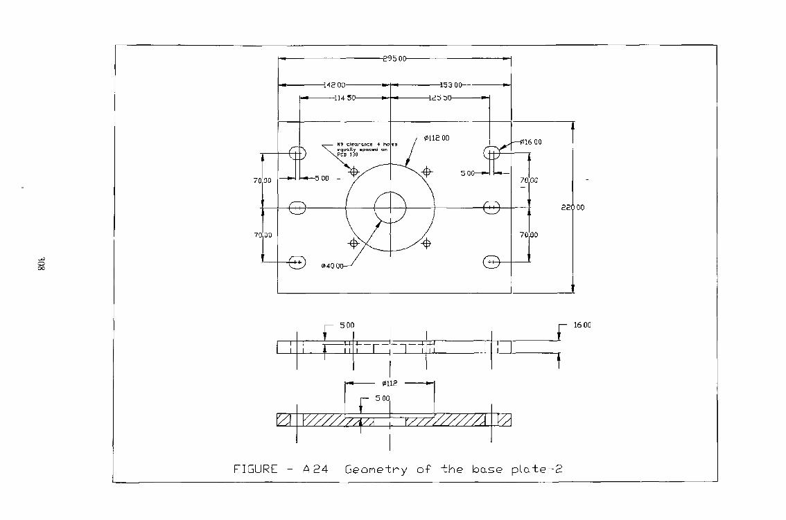
- Dimensions of the left column- Details of the back column- Details of the base plate- Position of the keyway m the left ballscrew- Position of the keyway in the rignt ballscrew- Dimensions of the guide rod- Geometry of the steeped shaft- Details of the thin plates- Geometry of the top cover plate- Details of the linear ball bearing- Details of the torque-tension shaft- Geometry of the torsion shaft- Details of the bottom face of the torsion shaft- Geometry of the square drive- Geometry of the adjuster- Geometry of the nut-1- Details of the nut-2- Schematic diagram of a Moog brushless servomotor- Dimensions of the timing pully- Details of the timing belt- Geometry of the base plate-1- Details of the fiame-1- Details of the spur gears- Geometry of the base plate-2
XIII
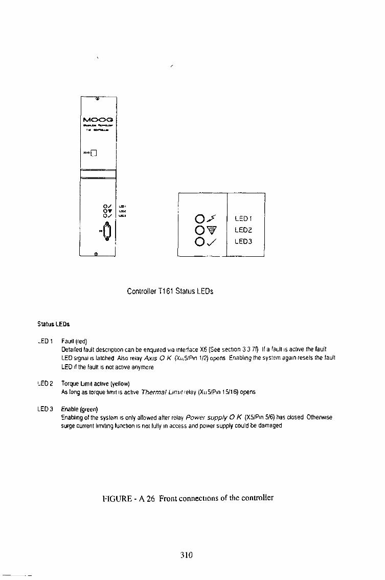
Figure - A 25 - Details of the frame-2 309Figure - A 26 - Front connections of the controller 310Figure - A 27 - Front connection of the power supply unit 311
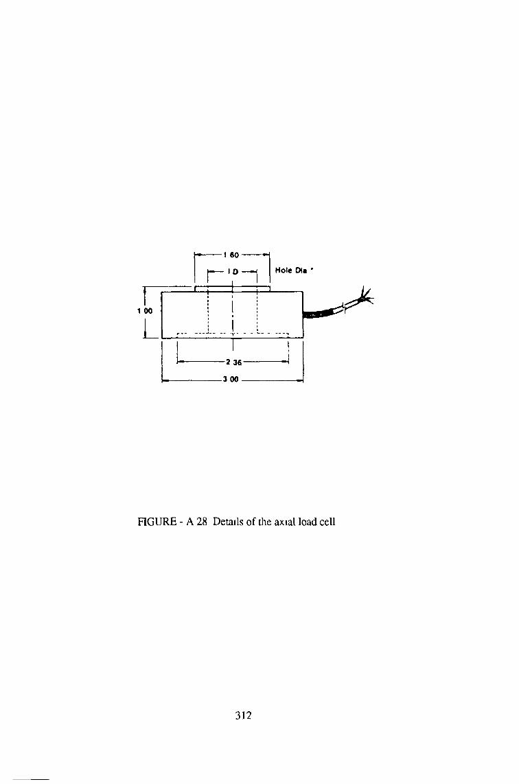
Figure - A 28 - Details of the axial load cell 312
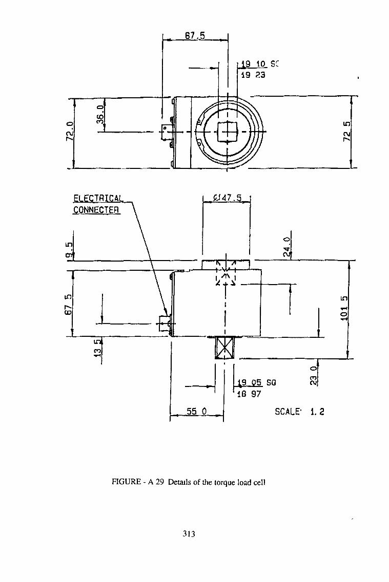
Figure - A 29 - Details of the torque load cell 313
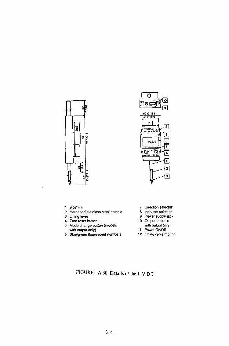
Figure - A 30 - Details of the L V D T 314
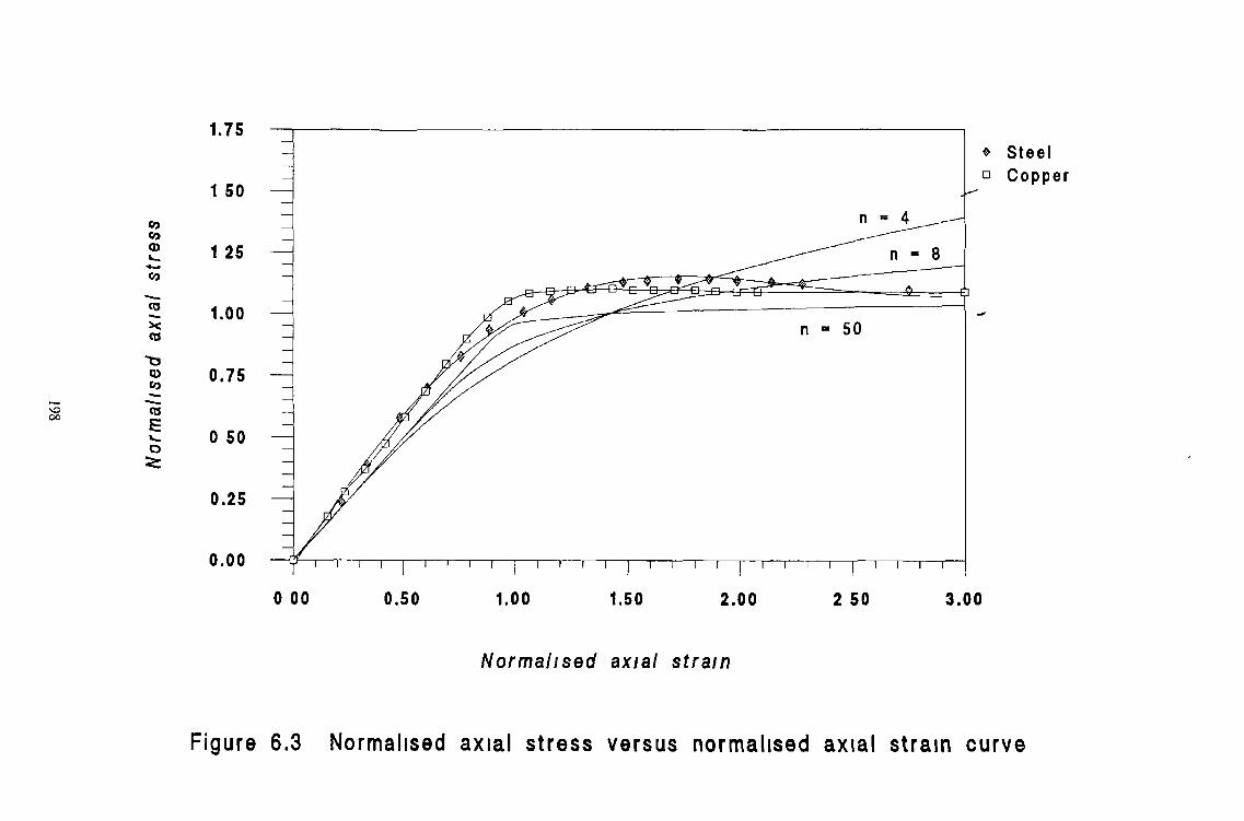
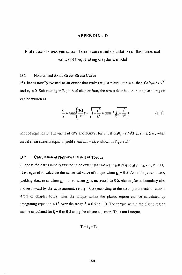
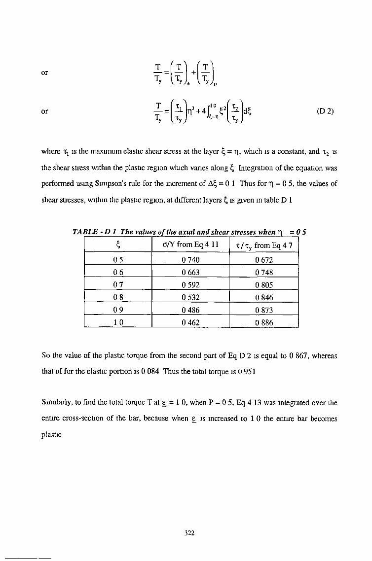
Appendix - DFigure - D 1 - Normalised axial stress versus axial strain curve of Eq - 4-6(a) 323
Appendix - EFigure - E 1 - Stress components at a point in loaded body 334
Figure - E 2 - Effect of loading path on plastic strain 334Figure - E 3 - Idealized stress-strain curves 335Figure - E 4 - Stress distributions for a non-strain-hardening and a strain
hardening material335
Figure - E 5 - Torque versus angle of twist/unit length curve 335
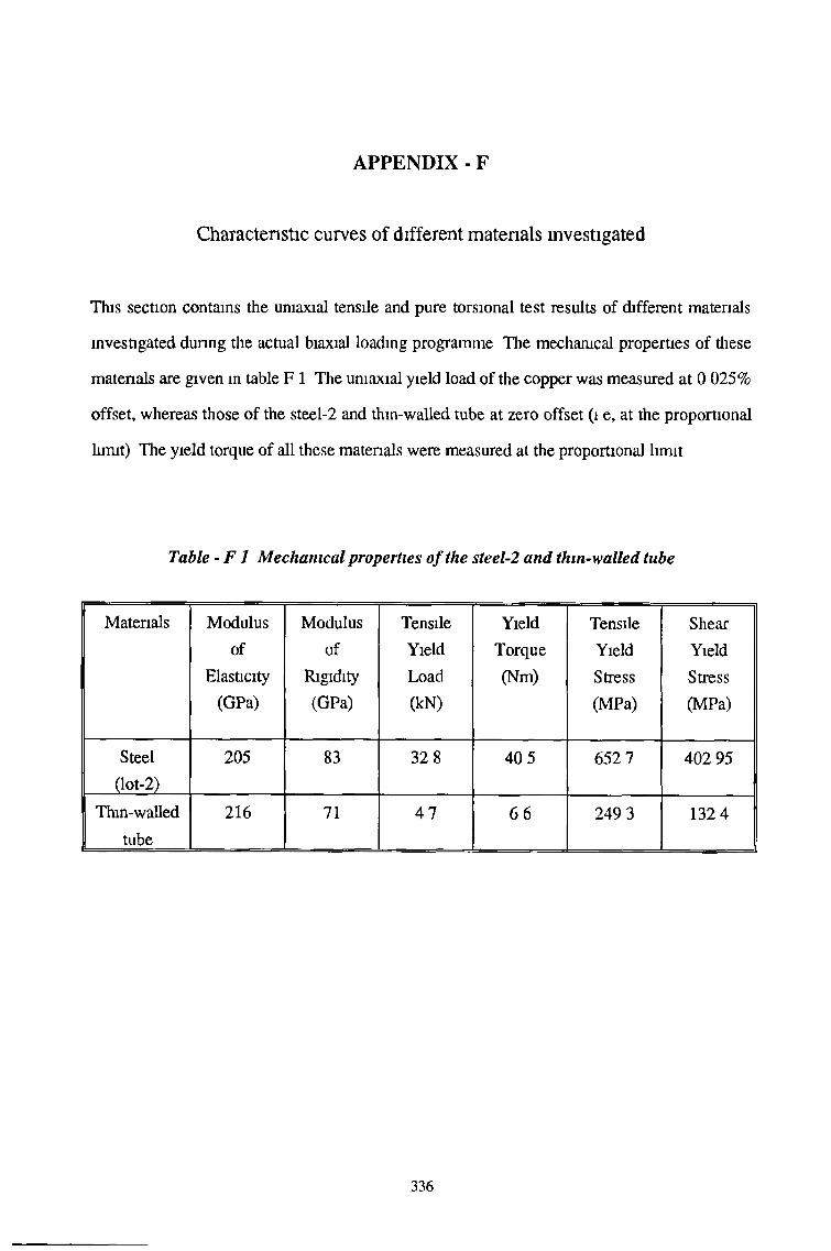
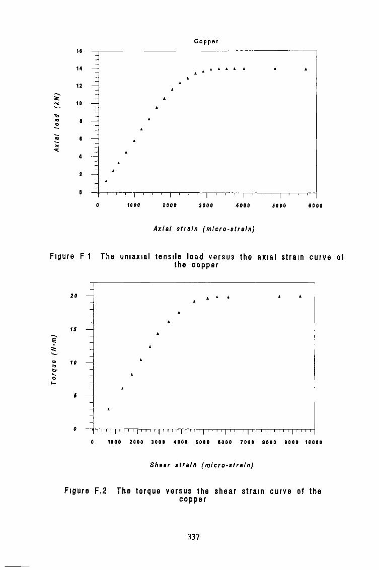
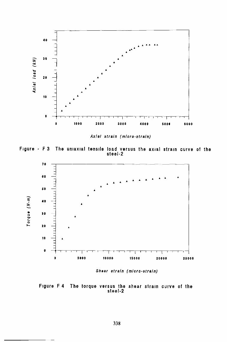
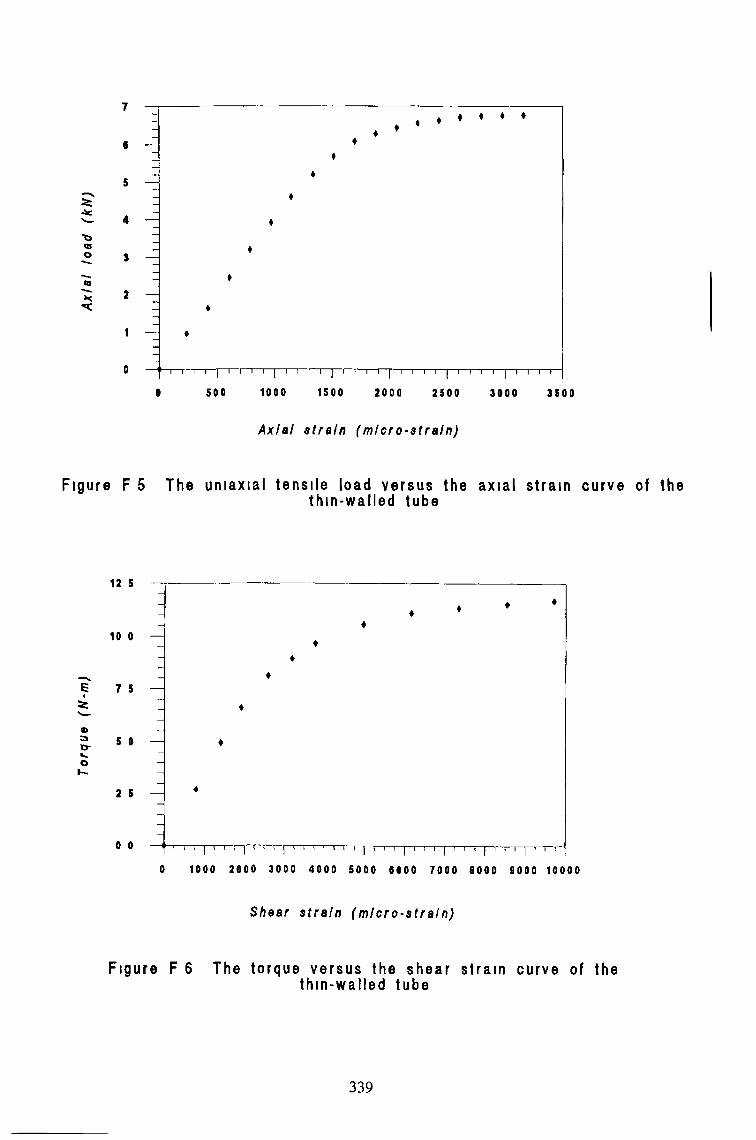
Appendix - FFigure - F I - The uniaxial tensile load versus axial strain curve for copper 337Figure - F 2 - Pure torque versus shear strain curve for coppe 337Figure - F 3 - The uniaxial tensile load versus axial strain curve for steel-2 338Figure - F 4 - Pure torque versus shear strain curve for steel-2 338Figure - F 5 - The uniaxial tensile load versus axial strain curve for
thin-walled tube339
Figure - F 6
Chapter Three
- Pure torque versus shear strain curve for thin-walled tube
LIST OF PLATES
339
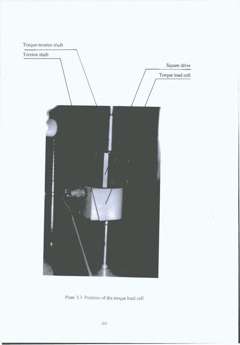
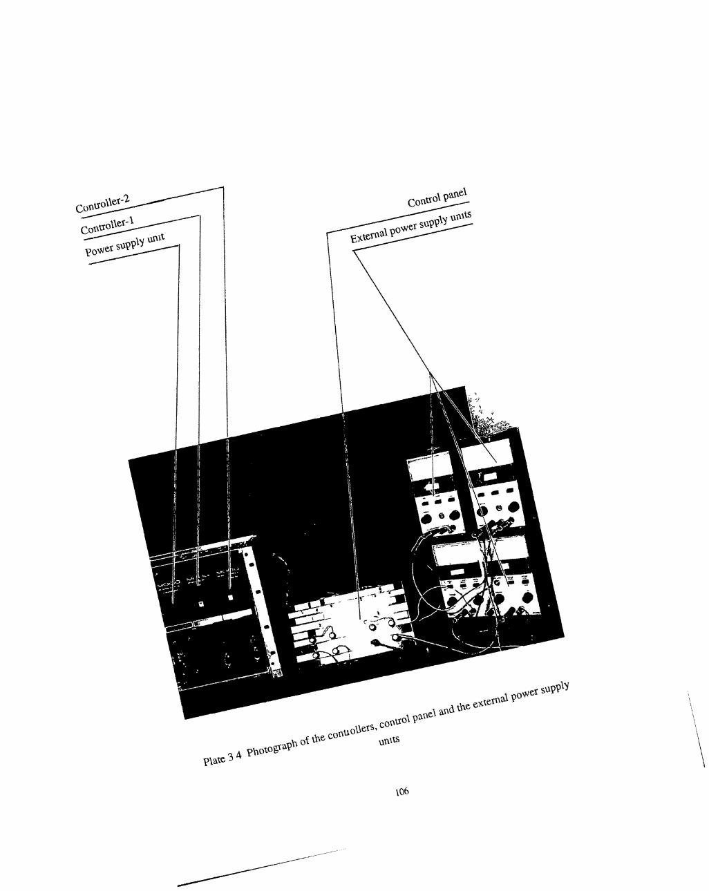
Plate - 3 1 - Details of the torque-tension machine 103Plate - 3 2 - Position of the specimen in the gripper 104Plate - 3 3 - Position of the torque load cell 105Plate - 3 4 - Photograph of the controllers, control panel and the external
power supply units106
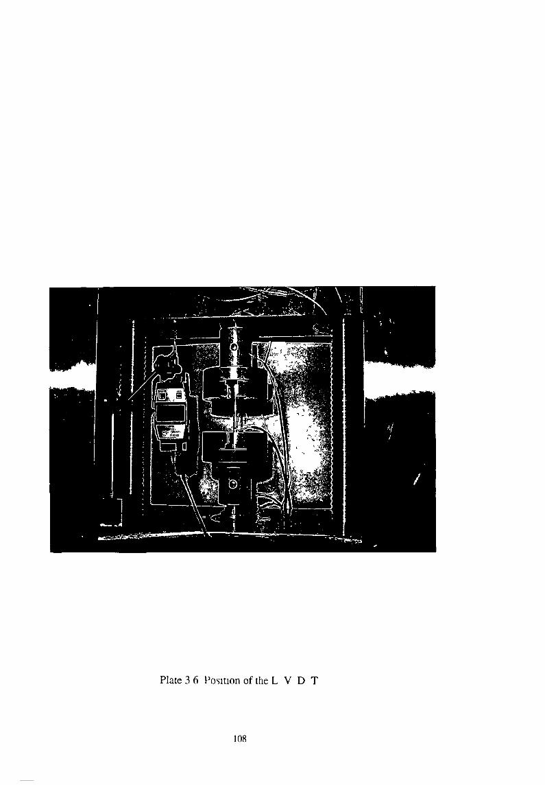
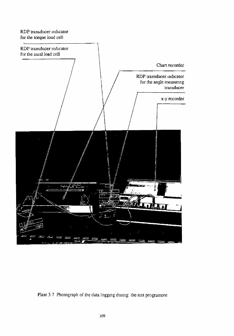
Plate - 3 5 - Position of the angle measuring transducer 107Plate - 3 6 - Position of the L V D T 108Plate - 3 7 - Photograph of the data logging during the test programme 109
XIV
Chapter FivePlate - 5 1 - Photograph of the digital strain indicator and the switch and 163
balance unitLIST OF TABLES
Chapter ThreeTable - 3 1 - The specifications of the torque-tension machine 26Table - 3 2 - Details of the ball screw 29Table - 3 3 - Functions of various pins on the X|i7 connector 49
Table - 3 4 - Set-up limits of torque and speed in motor-1 and motor-2 51Table - 3 5 - Connection of power connector X|i4 53Table - 3 6 - Specification of the taper roller bearings 63Table - 3 7 - Specification of the cylindrical roller beanngs 63
Chapter SixTable - 6 1 - Mechanical properties of the steel (lot-1) and copper 168
Appendix - FTable - F I - Mechanical properties of the steel-2 and thin-walled tube 336
XV
CHAPTER ONE
INTRODUCTION AND JUSTIFICATION
1.1 JUSTIFICATION AND IMPORTANCE OF THE WORK
In metal forming processes, such as forging, extrusion, drawing, rolling etc , where very large
plastic strains and deformations occur, elastic strains aie usually neglected and the materials
can be assumed to be perfecdy plastic On the other hand, where the plastic strains are of the
same order of magnitude as the elastic strain, the problems are elasto-plastic problems These
types of problems are of prime importance to the structural and machine designer With the
great premium placed on the saving of weight in aircraft, missile, and space applications,
designers can no longer use large factors of safety and designing must be done for maximum
load to weight ratio, and this inevitably means designing into the plastic range
In assessing the ultimate load carrying capacity of some structures, it is frequently necessary
to consider the elasto-plastic behaviour of structures These (ultimate loads) can be calculated
from a knowledge of load-defoimation relationships for the individual elements of which the
structure is composed Deformation in the elasto-plastic range is much more difficult to
calculate than elastic deformations because relationships between the stresses and strains are
non-linear and are dependent on the loading history Furthermore, the stress distribution in
most structural members loaded into the elasto-plastic range is also difficult to determine,
because the shape of the elastic-plastic interface is itself related to the stress distribution and is
therefore unknown until the complete solution is found However, for a solid circular rod
subjected to combined torque and tension, tins restriction is removed since the shape of the
interface must be annular to preserve axial symmetry
1
Structural elements and machine components are usually designed so that material does not
yield under the expected loading conditions. The magnitude of the stress, which causes the
material to yield under uniaxial or combined loading, can be well predicted by using various
theoretical "yielding criteria". Once the yielding has started, the material is said to be either in
plastic or elastic - plastic condition depending on the type of material used. If a circular steel
bar is subjected to combined axial load and torsion, yielding does not occur until the
combined stress state reaches the critical value; i.e., the yield locus of that particular material.
Upon reaching the yield locus, if further axial load and/or torque is applied, plastic flow starts
in the material. The linear elastic torsion theory stipulates that the maximum shear stress
occurs at the outer fibre of the material, accordingly for problems concerning the
simultaneous application of axial load and torque, yielding takes place at the outer fibre of the
specimen.
Upto the yield point, the combined loading effects can be well explained by various theoretical
equations and by different yielding criteria. But the response of the material is difficult to
explain, when the axial load or torque is applied beyond the combined yield stresses, holding
one parameter, either torque or axial load, as constant. If the axial load is increased
continuously to beyond the combined yield stress, holding the angle of twist constant for a
certain pre-torque within the elastic range, the manner in which this axial load will effect the
magnitude of the initially applied torque requires careful study. Similarly, when both the axial
load and the torque are successively applied to a pre-torqued or pre-loaded specimen the
response becomes very complex. As it is well known that the behaviour of the material is
strongly dependent on the strain path in the plastic region, so that when a solid rod is
subjected to the above mentioned types of loadings, it is difficult to predict the exact response
of the material both theoretically and experimentally, where the latter needs detailed
experimental facilities. However, most of the existing research works, concerning the elastic-
plastic response of materials, have been conducted using thin-walled tubes for the sake of
simplicity of analysis.
2
In this research programme, the detailed theoretical and experimental investigations regarding
the response of a circular rod in the elastic-plastic range under combined tension and torsion
have been earned out To this end, a torque tension machine has been designed, manufactured
and commissioned which facilitates both simultaneous and independent applications of
torsional and tensile loads to the specimen
1.2 INDUSTRIAL RELEVANCE OF THE WORK
Assembly applications can be segmented into two categories One is the joint in which
clamping force is being supplied by the fastener to prevent any movement to the mating part
where performance and reliability are a function of the load In the other category, the
fastener is used as a pin or nvet This type of joint is designed to allow motion in either of the
two directions one is a scissors type motion and the other is a flexing type application Bolts
and nuts, screws fall into the first category
Fastening bolts are still the most frequently used method in joint technology This is the case
for many components used within the motor, aerospace, and machine tool industnes
Designers are reducing the margin of safety which is built into a machine This change is
accountable specially to an aerospace industry which works to a safety factor of 1 1 as the
maximum expected load [1] This forces fastening systems into more acute performance
ranges Moreover, with fasteners and fastener assembly becoming a very expensive part of the
end product, utilising the maximum capability of the system is a must A company can no
longer afford to use only 50% of the pi oof load of a bolt due to poor torque-tension control
Consequently, factors affecting the design and integnty of bolted joints are of considerable
industnal interest
Considerable investigations are still being carried out into bolted joints, specially into the
quality of the tightening involved and into the bolt itself Bolted joints still pose many
3
problems for engineers, since they involve complex parts working under severe and often
limiting conditions The financial penalties which result from their failure are disproportionate
to their intrinsic cost, and this fact justifies the attention which must be paid to them Recent
investigations carried out into numerous failure cases have shown without doubt that such
problems and/or incidents are largely due to the misappreciation of the proper response of
fastener during tightening and the change it undergoes with additional external load or over
tightening
The design and assembly of bolted joints must assure that the joint remains tightly clamped
and the fastener is capable of withstanding the static and dynamic loads that are applied
Service performance of a joint depends on many factors, such as the properties of the
fastener and the structure being clamped, response of the bolt and joint under additional load,
the tightening process and, not last but least, on the type of lubncation used In establishing
the design capability of a bolted joint, some frequently asked questions are to be answered,
such as
(1) How tight should the bolt be and what assurance is there that the assembly process can
consistently achieve this level of tightening ?
(u) What level of external load will cause the joint to open ?
(m) What load is felt by the bolt when the service stiesses aie applied to the fastened
assembly **
(i v ) What are the properties of the bolted joint under dynamic loads or fatigue conditions ?
With recent improvements in the control of fastener tightening and new knowledge of bolt
and joint properties, these questions merit detailed attention in order to obtain the maximum
performance at minimum cost [2] Now it has been found that by tightening the bolt to the
yield point, not only are higher clamping forces produced but more consistent clamp loads are
obtained [3-5] A bolted joint tightened with yield control to the bolt torque-tension yield
4
point can withstand very substantial external loads without deterioration Typically, a
concentric joint can have an external load equal to the proof load of the fastener applied [2]
The load felt by the bolt when the service stresses are applied depends not only on the
tightening procedure but also on the fnction condition of the fasteners The traditional torque
control method of tightening bolts has been shown to give very inconsistent levels of achieved
clamp loads when a number of fasteners are tightened to the same torque [3] The
requirement of consistency in clamp load, coupled with the desirability of obtaining the
highest clamp loads possible has led to the development of a new tightening system referred
to as "Joint Control Tightening" [6], where the bolts are tightened to yield points for the
reasons mentioned earlier
It has been established that as the fnction condition at the fastener threads and the underhead
bearing surface changes, the proportion of the applied torque available to develop the clamp
load also changes [7] The higher the values of fnction co-efficient at these areas, the lower
the values of resulted clamp loads in the bolts as now more of the applied torque is used to
overcome the thread fnction So bolts are yield tightened to reduce the scatter of the resulted
clamp load in bolts and to attain consistency in preload whereas bolts are lubncated to
increase the clamp load in the joints Higher preloads are necessary not only to maintain a
tight joint, which is the pnmary objective of a joint assembly, but also to increase the fatigue
resistance of the bolts In a hard concentric joint, preload is the predominant factor governing
fatigue Whereas in an eccentncally loaded joint, the preload is the major factor controlling
the additional bolt load More over at higher preload, the additional load felt by the bolt due
to the application of external load, is less than that at lower preload [2]
It has also been found that even after yield tightening the bolts, there is a reserve of strength
between the as tightened tensile stress and its uniaxial yield strength [8] That means, if further
external tensile load is applied to a yield tightened bolt, it does not fail or reach its tensile yield
5
point instantly, but can withstand a certain amount of additional tensile load During this
penod, 1 e , when external loads are applied to the "torque-tension" yield tightened fasteners,
all bolts behave elastically As it is well known that during the tightening process a fastener is
subjected to torsional as well as axial stiess applied simultaneously Subsequently, when the
assembly or the joint is subjected to external load, the fastener is subjected to additional axial
stress or axial and bending stress In this case, wheie the external load in the joint results in
additional axial load in the pre-loaded fastener, it is expected that the plastic yielding would
take place at a total yield load which is less than that if there is no torsional stress present
So it was felt necessary to carry out investigations to know how the external tensile load
affects the magnitudes of the applied torque or how further application of the torque affects
the magnitude of the resulted preload in a bolt in the elastic and plastic range To avoid the
complex relationships among the tightening torque, friction co-efficient and pre-load, which
results in a bolt, as already discussed earlier, a simple cncular rod ( fastener like structure) has
been used as a specimen
This research programme has been undertaken to carry out detailed experimental
investigations regarding the elastic-plastic response of a circular rod subjected to successively
applied torsional and tensile stresses During bolt tightening, as the main stresses developed
are only the tensile and shear stresses, as such the present research investigation is a similar
condition to bolt tightening However, during the tightening process other stress components
do anse due to the effects of the helix angle and the geometry of thread, the effect of these
stresses are not being considered in the present study because of simple design of the
specimen
6
1.3 AIMS OF THE STUDY
The main objectives of the current work can be summarised as follows
(1) To design, build and commission an instrumented mechanical torque-tension machine
which is capable of applying biaxial loads, such as torque and tension, either
simultaneously or independently under different controlled conditions
(n) To carry out a detailed experimental investigation to observe the elastic-plastic response
of a pre-stressed rod (1 e , either torque or tension) when subjected to subsequently
applied parameters (1 e , either axial load or torque) under different controlled and
boundary conditions, and to enhance better understanding of the mechanics of such
response
(m) To verify the experimental results obtained during the biaxial loading with theoretical
models
In order to achieve the above mentioned objectives, the following method of approach has
been adopted
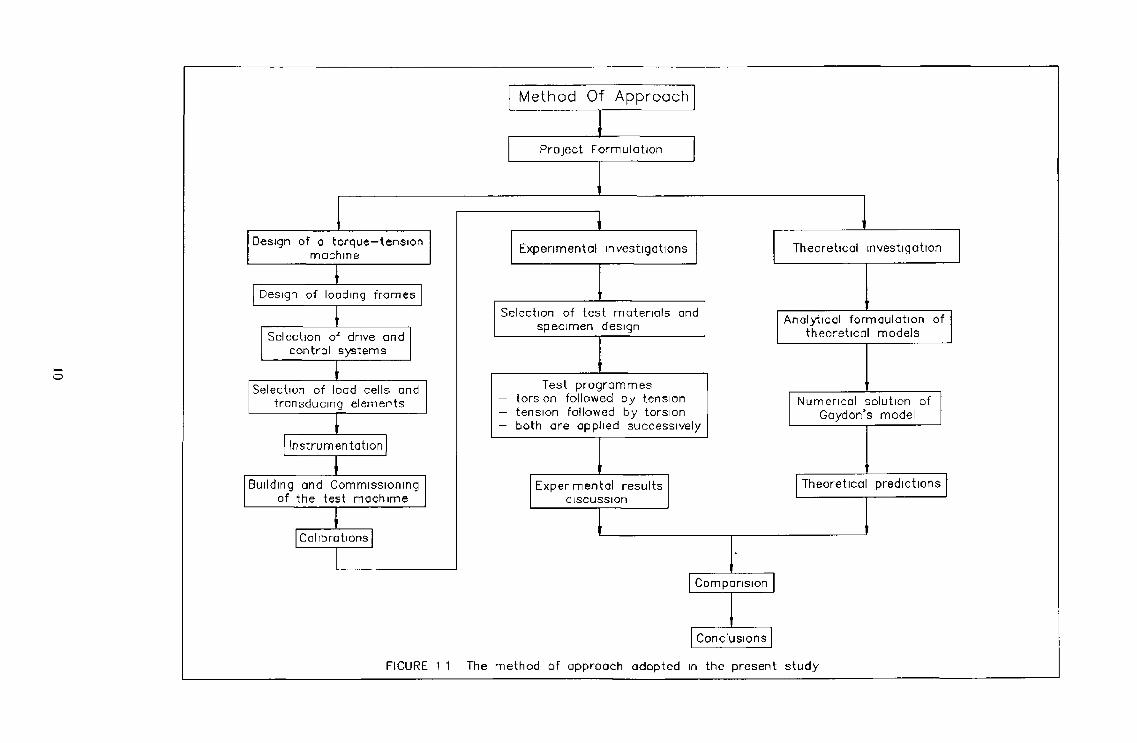
1.4 METHOD OF APPROACH
The method of approach, shown schematically in figuie 1, has been divided into three mam
sections The first one was devoted to design, manufacture and commissioning of an
instrumented mechanical torque-tension testing machine to enable the application of biaxial
loading under controlled conditions The second was wholly concerned with the experimental
investigations where solid rods were subjected to complex non-proportional biaxial loading
paths In these paths, elasto-plastic torsion followed by tension, keeping angle of twist
constant, and elasto-plastic tension followed by torsion, holding corresponding axial
displacement constant, weie examined Other loading paths, where the initial axial loads and
the torques were maintained constant, and where the torque and the axial load were applied
successively, were also studied The expenmental piogramme also considered the biaxial
7
loading of thin-walled steel tubes In the thud, the experimental results were compared with
two different analytical models, developed by Gaydon [18] and Brooks [20], respectively
In building the machine, the main frame along with its necessary auxiliary components were
designed and manufactured, proper drive and conti ol systems were selected, and appropriate
load cells and transducing elements were attached to it The machine was then commissioned
and calibrated In the theoretical investigations, a numerical solution scheme was developed
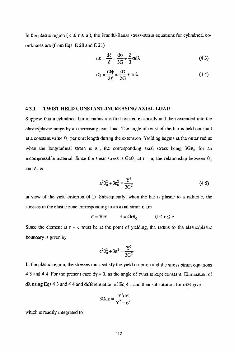
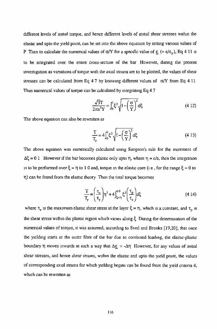
along the lines of Gaydon
The experimental investigations under combined loading were carried out according to the
following steps
(I) Initial torque of known level, withm the elastic range of the material was applied, and
then, axial load was gradually incieased beyond the uniaxial yield load, holding the
corresponding angle of twist constant
(II) Procedure (1) was repeated except the applied initial torque, rather than angle of twist,
was maintained constant
(m) Initial axial load of known level, within the elastic range of the material, was applied and
then, torque was gradually increased beyond the yield torque, keeping the initial axial
displacement constant
(i v ) Procedure (m) was repeated except, in this case the initially applied axial load, rather
than axial displacement, was maintained constant
(v) Initial torque of known level, within the elastic range, was applied and then, holding the
corresponding angle of twist constant, axial load was gradually increased until the specimen
yielded due to the combined loading Subsequently, small increments of torque and axial load
were successively applied beyond the combined yield point, holding the axial displacement or
the angle of twist constant m an alternate manner
(vi) Initial axial load of known level, within the elastic range of the material, was applied and
then, holding the corresponding axial displacement constant, torque was gradually increased
8
until the specimen yielded due to the combined loading Then, axial load and torque were
successively applied beyond the combined yield point, holding the angle of twist or axial
displacement constant in an alternate manner
1.5 LAYOUT OF THESIS
This thesis has been divided into seven chapters Following this introductory chapter, chapter
two gives a critical review of the relevant literature Chapter three is devoted to the design,
manufacture and commissioning of the test ng This chapter also contains the details of
various drive, control and data acquisition systems used in this machine Chapter four gives
the analytical formulation of different theoretical models used to compare with the
experimental results It also contains an analytical model to calculate the stiffness of the
torque-tension machine Chapter five is devoted to the experimental procedures followed
dunng the tests and, for the selection and design of the test specimen This also contains the
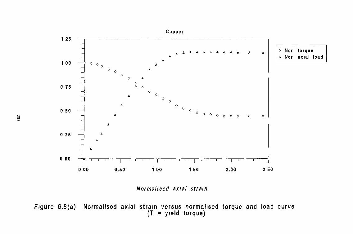
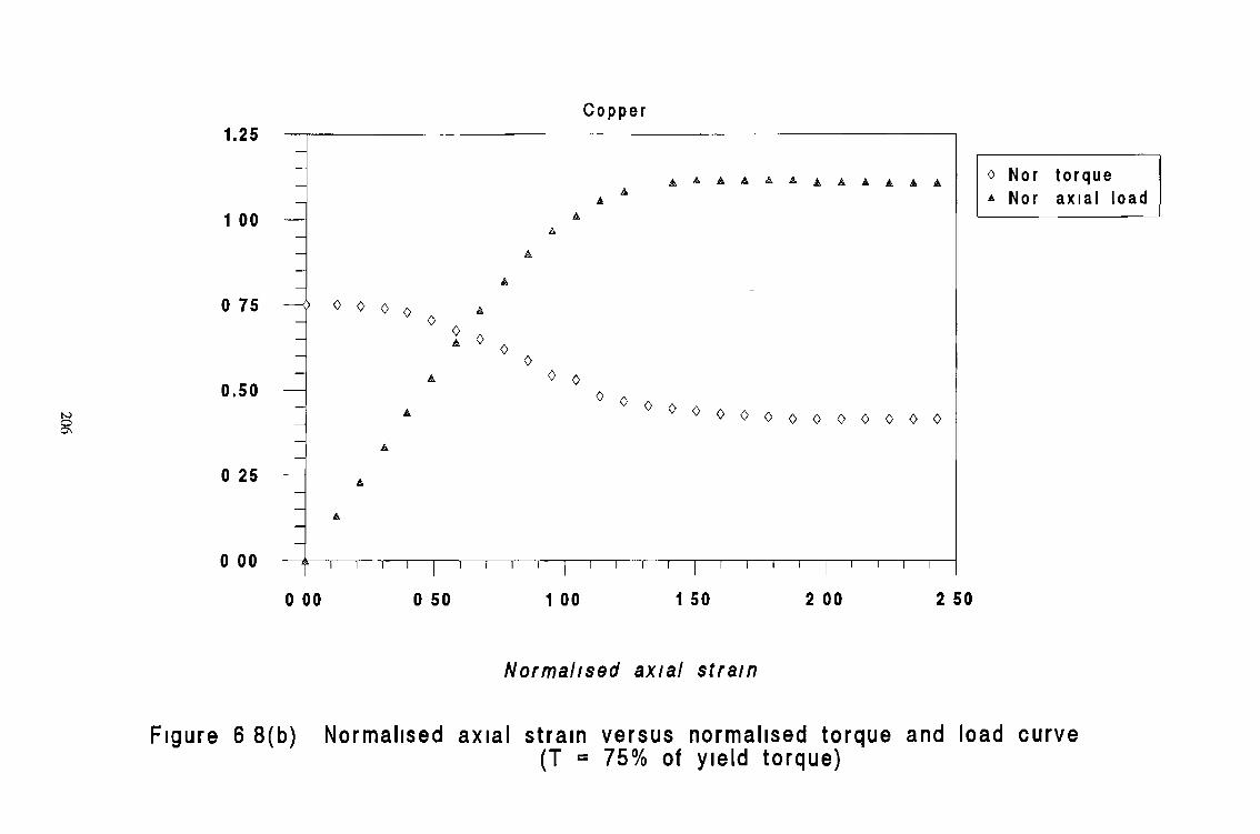
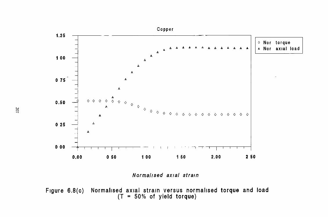
calibration results of the testing machine Chapter six is devoted to the analysis of the results
and discussion and, also for the comparison of the experimental results with the theoretical
predictions Chapter seven mentions the summary of the findings of the research and
recommendation for future works
9
FIGURE 1 1 The method of approach adopted in the present study
CHAPTER TWO
LITERATURE REVIEW
2.1 INTRODUCTION
Most of the early experimental investigations under combined stresses and in the elastic-
plastic or in the fully plastic region have been carried out either to verify different analytical
and numerical solutions of the elastic-plastic or plastic stress-strain relationships, proposed by
various investigators, or to verify different yield criteria In most investigations, a thin walled
tube has been used as the specimen for the sake of simplicity However, as detailed
experimental work under combined torsion and tension involves complex loading histories,
and hence needs a proper testing machine, very few attempts have been made to conduct
similar types of experimental work This chapter provides critical review of the previous
investigations related to the present work for both solid and thin walled specimens
2.2 HISTORICAL PERSPECTIVE OF COMBINED LOADING IN
THE ELASTO- PLASTIC REGION
The conditions under which various materials begin to deform plastically have been the
subject of many experimental investigations during the last hundred years Among these,
investigations on various materials, which might be mentioned are, as outlined by Nadai [9],
the tests with ductile metals, rock materials, marble and sandstone under combined stress,
with zinc and steel, and concrete under combined stress Tests on iron, copper, nickel,
aluminium, lead, cadmium, mild steel, glass, brass and nickel-chrome-molybdenum steel were
also reported in reference [9]
11
The most detailed experimental investigation under combined stresses in the elastic-plastic
range have been carried out by Lode [10] He tested thin-walled metal tubes of steel, copper
and nickel, as outlined by Mendelson [76], under various combinations of longitudinal tension
and internal pressure to verify different yield criteria Lode devised a very sensitive method of
differentiating between the Tresca and von Mises yield critena by determining the effect of the
intermediate principal stress on yielding He introduced a parameter, called "Lode's stress
parameter" to account for the influence of the intermediate stress in the von Mises criterion,
which is the ratio of the difference between the intermediate stress and the average of the
largest and smallest stresses to half the difference between the largest and smallest stresses It
was shown that the experimental results have better agreement with von Mises criterion than
Tresca's
In the following year, Lode also carried out same type of expenments, as outlined by Hill
[11], to investigate the validity of the Levy-Mises strain-stress relations An approximately
constant ratio of axial and circumferential stresses was maintained in each test It was found
that the relation was valid to a first approximation, but despite appreciable scatter in the data
due to anisotropy (l e in many instances Lode's strain parameter was not equal to -1 in simple
tension, as it should be in an isotropic material from symmetry alone) in the drawn tubes, the
results indicated a probable deviation from the Levy-Mises strain-stress relation
K Hohenemser [12] also earned out expenmental investigations to verify the validity of the
Reuss stress-stram equations He used pre-strained mild steel, as outlined in [11], to secure a
sharp yield point and reduce the rate of hardening to a value small compared with the elastic
modulus A cylindncal tube was twisted to obtain an approximately uniform distnbution of
stress at the point of yielding and then holding the angle of twist constant, the tube was
extended longitudinally Though one of the biaxial loading path followed dunng the present
expenmental investigation was similar to the above mentioned path, the idea of performing
the test was completely different In the present case attempt was made to observe elastic-
12
plastic response of a pre-stressed solid rod when subjected to different parameter, such as
torque or tension, whereas Hohenemser's experiment was performed to verify the validity of
the Reuss stress-strain equations However, no conclusion was found regarding the
Hohenemser’s experiment from any published paper Later on, Momson and Shepherd [14]
earned out similar expenments to venfy the validity of Reuss-Prandtl equations
Taylor and Quinney [13] used aluminium, copper, and mild steel tubings, which were very
nearly isotropic and stressed them in combined tension and torsion, primarily to venfy
different yield cntena Thin walled tubes weie first loaded in tension into the plastic range
then partially unloaded and twisted until some further plastic flow occurred The axial load
was held constant while the torque was increased, so that stiess ratios were not constant The
torque-twist or torque-extension diagrams were extrapolated back to zero twist or zero
extension to establish approximately, but fairly accurate, the torque at which plastic flow
recommenced The degree of anisotropy was kept within allowable limits by observations of
the change in internal volume of the tubes dunng pure tension By first straining each
specimen in tension, they were able to pre-strain the matenal by any desired amount and also
to detect anisotropy in the matenal Although Taylor and Quinney ignored the possibility of
an elastic increment of strain dunng plastic flow, they also found the same results regarding
the von-Mises yield cntena and concluded that the deviation from the von-Mises criterion
was real and could not be explained on the basis of expenmental accuracy or isotropy
Momson and Shepherd [14] subjected thin hollow tubes to tension and torsion to follow a
complex path of stress to compare the expenmentally found strain paths with those calculated
by Prandd-Reuss and Hencky stress-strain relations Here plastic and elastic strains were
comparable The matenal used was 5 percent nickel steel and 11 percent sihcon-alumimum
alloy They applied first tension, then holding the tensile stress constant, applied torsion,
followed by further tension and torsion to obtain various strain paths The measured
13
\
variations of length and twist were in substantial agieement with the predictions of the Reuss
equations
Siebel [15] overstrained a thin tube by simultaneous action of bending and twisting couples
He tested the validity of the Reuss stress-strain relations when the stresses and the stains were
not uniformly distributed The test results were found to be predicted very accurately by the
theory To investigate the rapidity of approach to the plastic-ngid yield point values, Hill et
al [16] used alloy steel bars of circular cross section which were strained in combined torsion
and bending In each test, the ratio of bending and twisting moments was held constant In
order to eliminate machining stresses, as far as possible, all the specimens were subjected to a
stress relief anneal after machining They compared their experimental results with the
calculated yield point of the bar and obtained upper and lower bound solutions The results
showed that the plastic-ngid yield points may be used in design calculations
Prager and Hodge [17] and Gaydon [18] developed analytical expressions for the stress
distributions and deformations of solid circular bars subjected to combined tension and torsion
in the elastic-plastic range In both cases the analysis was restricted to a material with a
specific Poisson's ratio (=1A)y i e , they did not take the effect of elastic compressibility The
latter author considered various combinations of twist and extension The Reuss equations
were used throughout and these were integrated, for different cases, to give the shear stress
and tension in the plastic range However, during the present study a numerical solution for
Gaydon's analytical model has been developed, which within the author's knowledge has not
been performed by any other investigator
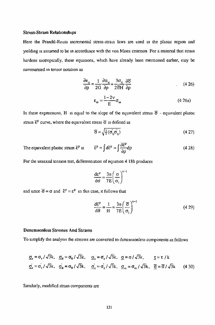
Brooks et al [19-20] examined analytically and numerically the behaviour of a circular bar
subjected to combined axial load and torque in the elasto-plastic range In reference [20],
Ramberg-Osgood curves were used to describe the material behaviour, and the analysis was
based on the Prandd-Reuss incremental stress-strain laws and the von Mises yield criterion
14
Brooks [20] obtained numerical results for both proportional and non-proportional loading
combinations Elastic compressibility was taken into consideration which was shown
negligible for all practical purposes
Naghdi et al [21] conducted experimental investigation with tubular specimen, made of 24 S-
T4 aluminium alloy, which were subjected to combined action of tension and torsion with
variable loading paths The loading was such that tension alone was followed by torsion and
permitted the determination of the initial shear modulus when twist began These tests were
performed to determine the initial anisotropy of the material tested The experimental results
were discussed in the light of incremental-strain theories of plasticity
In problems involving both elastic and plastic deformation, the plastic strain rates may vary
with position and time by several orders of magnitude even for constant total deformation
rates For certain metals and alloys, such large variations in plastic strain rate cause significant
changes of flow stress Meguid et al [22-24] carried out a number of investigations, both
theoretically and experimentally, under combined torque and tension for rate dependent
material Thin walled circular tubes of both elastic-perfectly plastic and work hardening
materials were used in their works In refeience [23], bilinear deformation paths of twist at a
constant rate followed by extension at different lates were examined to evaluate the plastic
flow of the material under abruptly-changing deformation paths and strain-rates Experimental
results were compared with the existing strain-rate dependent theory The experimental
results indicated that there exist appreciable differences between the von-Mises equivalent
stress versus equivalent plastic strain curves for the different bilinear paths investigated These
differences were attributed to the strain-rate sensitivity of the particular material However,
almost in all their experimental works they have considered only one non-proportional biaxial
loading path, l e , torsion followed by tension keeping angle of twist constant They did not
consider any other non-proportion al loadings as has been considered in the present study
Furthermore, they tested thin-walled tube not the solid rod
15
McMeeking [25] discussed the kinematics and stress analysis of the tension-torsion test of a
thin-walled tube at finite strain He formulated the relationships between increments of tension
and torque and increments of extension and twist for an elastic-plastic material at finite plastic
strain for the most common constitutive assumption He evaluated the validity of the Prandtl-
Reuss equations for different ranges of plastic strains (1 e , when plastic strains are very large
and when they are comparable with the elastic strains)
Investigations on the spnngback of plastically deformed material under combined torsion and
tension have been carried out by Narayanawamy et at [26] Rectangular bars of two different
materials have been used as the specimens These specimens were standard ASTM E-8
specimens with 2 inch gauge length Their experiments were of two types In the first set of
experiments, the bars were initially pulled at different level of axial strains in the plastic
region, and then, were twisted for different angles of twist At the end, both load and torque
were removed simultaneously and angular springback of the material was recorded The other
type of experiment was of opposite nature, i e , pre-torqued specimen was loaded by tension
They mainly investigated angular spnngback They concluded that the spnngback was
analytically predictable and expenmentally found that the twist followed by pull produced
smaller angular springback upon release of torque and force than that produced deformation
in the reverse order
Based of the kinematic hardening theory, Wei Jiang [27-28] conducted analytical
investigations regarding the elasüc-plastic response of thin-walled tubes subjected to
combined axial load and torsion Exact closed-form solutions were obtained for linear loading
paths Stress-strain relationships, together with the corresponding movements of the yield
centre, were discussed for both monotonic and vanable loadings The response of the tube
under non-proportional loading was shown to be path-dependent Authors of reference [29]
earned out similar type of investigations as mentioned above, where thin-walled tubes were
subjected to axial load and internal piessure, instead of torsional load
16
Experimental investigations under combined stresses have also been earned out to obtain the
initial and the subsequent yield loci for different matenals under different loading conditions
Though the mam concern of the present research was not on the development of the
subsequent yield loci, a few relevant works regaiding the above mentioned topic have been
presented here to give a much broader idea on the effect of combined stresses m the elasto-
plastic range Typical investigations, on the initial and the subsequent yield loci, conducted by
Naghdi [30], McComb [31], Ivey [32], Mair and Pugh [33], Phillips and his co-workers [34-
38], Tang [39], Bertsch and Fmdley [40], Marjanovic and Szczepinski [41], Shiraton et al
[42-44], Moreton et al [45], Rees [46-49] and Yeh [50-51], might be mentioned
Expenmental work investigating the subsequent yield surface was initiated by Naghdi,
Essengburg and Koff [30] In their expenments, tubular specimens made of 2024-T4
aluminum were initially pre-stressed m shear, and the shapes of subsequent yield surfaces
were determined m the first and fourth quadrant of a two-dimensional stress space All yield
surfaces corresponding to different pre-stress points were convex and elongated m the
direction of the pre-stress Also observed are the Bauschinger effect and a lack of cross effect
The lack of cross effect was also observed by McComb [31] who investigated the subsequent
yield surface for the specimens of 2024-T4 aluminum
Ivey [32] subjected a tubular specimen of 2024-T4 aluminum to combined tension and shear
with pre-straining in shear direction His results show considerable modification m shape of
the subsequent yield surface due to strain hardening A definite shrinkage of the size of the
yield surface was noticed Curvature near the pre-straining point was also found to increase
A general translation of the yield surface in the dnection of pre-straining was evident
Mair and Pugh [33] conducted a number of interesting tension-torsion tests on thin-walled
copper tubes, where the specimens were pre-strained m tension, partially unloaded, and then
strained in torsion Yield was defined by the Lode extrapolation technique The subsequent
17
yield surfaces were consistent with isotropic hardening accompanied by relatively slight
distortion Bertsch and Findley [40] conducted extremely accurate tests on thin-walled tubes
of 6061-T6 aluminum Seven subsequent yield surfaces with the same specimen were
obtained when yielding was defined by small offset stain
Phillips and co-workers in numerous papers [34-38] also reported that the subsequent yield
surfaces were convex and that cross effect was weak They subjected the specimens of
aluminium 1100-0 to pre-stressing in tension, m torsion, and in combined tension and torsion
Translation of the subsequent yield surface in the direction of pre-stressing was observed
Further, the yield surface changes its size in the direction of pre-stressing and becomes smaller
when moved away from the origin, but larger when directed towards the origin
Thin walled tubular specimen of annealed medium carbon steel was tested by Meguid et al
[52] where the specimen was subjected to combined torque and tension to obtain the initial
yield locus of the specimen Heie they obtained almost the entire positive quadrant of the
initial yield locus from a single run without unloading or reloading (neutral loading)
Particular attention was given to the effect of the axial strain-rate on the shape of these initial
yield loci
Rees and others [46-49] have conducted extensive investigations, both experimentally and
theoretically, on the development of the yield locus considering biaxial loading cases
Moreton et at [45] conducted expenmental investigation where tubular specimens were
subjected to combinations of internal pressure, axial load and torsion Their experimental
results were compared theoretically by the author of reference [49]
Han and Yeh [51] have detenmned expenmentally the initial and subsequent yield surfaces of
annealed AISI type 304 stainless steel in the axial-torsional stress space Three loading paths
18
pure axial path, pure torsional path, and proportional axial-torsional path were investigated
Each path included loading, unloading, and reloading state
2.3 REVIEW WORK ON BOLTED JOINTS
It has already been mentioned that during bolt tightening the main stresses developed are
combined tensile and shear stresses and hence some previous works regarding the response of
fasteners and their joints under load are presented in this section
Most theoretical and experimental investigations within this area have been conducted for the
purpose of improving the performance and reliability of the fasteners and their joints
Historically, Archimedes in 250 B C developed and recorded the first spiral screw and used
it for lifting irrigation water However, it was not until the middle of the 15th century that
threaded fasteners were used for assembly [53] It was the advent of the industrial revolution,
however, that nuts and bolts became commonplace as fasteners Many invenuons of the time
relied extensively on threaded fasteners Among them were James Watt's steam engine, James
Hargreave's spinning jenny and Eh Whitney's cotton gin [54-55] Most of the early
investigations regarding the fasteners were devoted to the development of uniform and
standard threads, such as Whiteworth thread, Sellers thread or ISO thread, which are now
extensively being used as standard thread
Over the past two decades, the demands for assurance of quality and reliability in engineering
structures or components have steadily increased To improve these, in mechanically fastened
assemblies, detailed analysis of bolts and bolted joint has been earned out by many
investigators Fasteners' weight as well as the weight of components may be reduced by any
of the following ways by choice of material [56], subjecting the fastener to high design
stresses, i e , minimise fastener size [57], and by reducing the matenal content of the bolt's
19
head as investigated by Landtl [58] Extensive developments have taken place in the design of
the fastener itself with the rolling of threads after heat treatment [59]
Gardiner [1] investigated the various factors that effect the torque-tension relationships of
fasteners during the tightening process He mentioned that the torque-tension relationship was
affected by tangible (physical item) and intangible variables (assembly method) Tangible
factors were, plating conditions of the threads and beanng surfaces, hardness of the
components, resilience of mating material, grade and class of fit, and lubrication Intangible
factors were, operation performance, method of assembly and tool driving speed He
tightened the fasteners using zinc plated and cadmium plated nut and found that the torque
needed to reach a similar load was almost twice as much for the zinc plated hardware than for
the cadmium plated one
A dynamically loaded joint fails in most cases either by fatigue or by rotation loosening of the
fasteners Even the fatigue failure is often initiated by partial loosening Junker [60]
investigated the self-loosening of pre-loaded bolted connections when subjected to vibration
He applied various desired levels of vibration, which closely simulated the actual conditions,
in a pre-loaded joint by means of a vibration machine Whilst Goodiner and Sweeney [61] as
well as Sauer et al [62] tested only axial dynamically loaded connections, Junker generated
transverse forces and displacement as well as combinations of transverse and axial force He
has proposed special locking features to resist vibration It was found that the dynamic
transverse forces were more undesirable than dynamic axial forces Axial forces cause relative
movements through expansion of the nut thread, whereas, transverse forces cause relative
movements through rocking action of the screw in the internal thread or rocking motions of
the nut on the external thread
The primary objective of tightening a fastener is to develop sufficient clamping load to form
and maintain as essentially solid joint even when working loads are applied Since the resulted
20
preload in the bolt not only depends on the friction but also on the methods of tightening
processes, a number of investigations have been carried out to select the proper tightening
process for a desired preload
Boys and Wallace [6] have introduced a new tightening control system, called "joint control
system", where bolts are tightened to yield irrespective of the total torque required and
lubrication conditions The system operates by sensing the gradient of the torque-rotation
characteristics and detects the yield point of the fasteners It does not require pre-set control
of torque or rotation angle as required by other tightening control processes such as "torque
control" or "angle control" process Their results showed that the system has increased bolt
clamping loads and reduced their scatter very significantly Finkelston and Wallace [3] also
investigated detailed analysis of the bolted joint about the working loads imposed on the joint
and the stresses felt by the bolt
Sorel and other [63] have introduced a new method for measuring the value of the resulted
preload more accurately during bolt tightening The tightening tension can be measured by an
ultrasonic impulse method using echographs with a time basic They have shown that
inaccuracy in the tightening measurement was less than ± 5% if the tested bolts have met
some simple geometrical criteria
A test programme was designed and executed by Becker and others [64] to study the
accuracy and precision of a bolt torquing system which tightens the bolts to their torque-
tension yield point The test progiamme compared bolt preload values to both the axial yield
point and to the rotation torque applied to the bolt head The test programme also included
measuring the permanent elongation of the bolt to verify the performance Results showed
that parts of this test programme can be used to verify the accuracy and precision of the bolt
torquing system in the manufacturing environment
21
In reference [65], the authors investigated the plastic region tightening method applied to the
cylinder bolts in developing the new 2 0 litre and 2 2 litre diesel engines The bolts were
tightened by "angle controlled tightening method" to bring the bolts' load into the plastic
region They used bolts with different shank diameters and with different tensile strength The
test results indicated that the plastic region tightening method made it possible to raise the
minimum bolt load by 50% and reduce the bolt load variation to about one half as compared
with the torque controlled method Frictional effect was also largely eliminated They
proposed that, although the bolt's fatigue strength decreased as the plastic lengthening
progressed, thread rolling after heat-treatment and well-finished thread root radius made it
possible to provide satisfactory fadgue strength in the plastic region
Maruyama and Nakagawa [66] carried out experimental studies on the behaviour of the
bolted joints in elastic and plastic region separately Firstly, the direct tension test of the bolt
under uniaxial load was carried out Secondly, the bolted joint was tightened in elastic or
plastic region and then axial load was applied to that tightened joint after screwing the joint to
a material testing machine In another similar test, at first the bolt was tightened to a certain
torque and then the torque in the threaded portion was reduced to zero, by untightening the
bolt by a few degrees Axial load was then applied to that pre-tightened bolted joint The
results showed that threaded part torque has little influence on the axial tension-elongation
curve, and that the curve under external loading rapidly approached the curve of the single
bolt regardless of whether or not the torsional stresses were eliminated by joint springback or
backward rotation before the external load was applied It was also found that the joint can
withstand higher working loads when bolts were tightened into the plastic region
Newnhan et al [8] also drew similar conclusions regarding the influence of torque on the
uniaxial tensile strength of bolt Here bolts were tightened to torque-tension yield point only
and external load was applied by a hydraulic cylinder
22
Chapman and others [2] investigated the static and dynamic strength of bolted joint tightening
the bolts to their yield points by using "joint conti ol tightening system" Firstly, the bolts were
tightened to their torque-tension yield points and then holding the angle of twist constant,
external tensile load was applied gradually until the bolts failed by their uniaxial tensile load
They made similar conclusions regarding the static loading of the bolts, as found by the
investigators in reference [66] Moreover, they also found that all bolts behaved elastically
when external loads were applied to the joints even when the fasteners were tightened to their
yield points Results about dynamic tests showed that fatigue strength increased with the
preload and high fatigue bolts gave an improvement over standard fasteners at all preloads
Hagiwara et al [67] and other investigators [68,69] conducted almost the same type of
investigations regarding the behaviour of the bolted connection tightened into the plastic
region with various types of clamp joint Investigators referenced in [68] and [69] also
investigated experimentally the influence of clamping force on the fatigue strength of bolts
Nakagome et al [68] also studied the influence of the thickness of the clamped parts taking
force ratio (axial force developed in the bolt body/external load) into account It was found
that when bolt was clamped in the plastic region, the fatigue limit of the bolted connection
was improved and the variations of the clamping force, axial load and force ratio were hardly
recognised They also concluded that force ratio decreased as the thickness of the clamped
part increased
Monaghan and Duff [7] and Monaghan [70] investigated the effects of external loading and
lubrication on a yield tightened joint It was found experimentally that lubncation conditions
dramatically affected the magnitude of the maximum clamp load achieved on the joint and the
torque distribution of the fasteners
23
Harm [71] earned out experimental investigations on bolted joints where bolts were initially
pre-torqued in the elastic range by means of an electronic hand torque wrench and then
external tensile loads were applied holding angle of twist constant Tensile load was applied
with the help of a hand hydraulic pump He noticed that the torque started decreasing when
the combined stresses in the bolt bodies reached the yield stress in tension However, because
of limited testing facilities in his set-up, and as he used shear strain gauge to monitor the
decrease of torque dunng the plastic deformation, it was not possible to explain the physical
mechanism by which the torsional stress disappeared and its associated energy dissipated It
was also not possible to maintain a specific torque or axial load or axial displacement constant
for different biaxial loadings of the bolted joints
Tsuji and Maruyama [72-74] have investigated the behaviour of the bolted joints tightened
into the plastic region In reference [72], they have proposed a new estimation method for the
interaction curve of the threaded portion based on the flow theory, instead of the traditional
one based on the local yield condition Experimental results [73] revealed that the new
method is superior to the traditional one
24
CHAPTER THREE
DESIGN, MANUFACTURE AND COMMISSIONING OF THE TEST RIG
3.1 INTRODUCTION
As part of this research work an instrumented torque-tension machine was designed,
manufactured and commissioned This machine enables the application of biaxial loads under
controlled conditions It can apply both torque and tension either simultaneously or
independently to specimens of various cross-section Suitable drive and control systems were
selected for the machine Appropriate load cells and transducing elements were attached to it
to allow the necessary data acquisition, by which parameters such as axial load, torque, axial
displacement and angle of twist, were monitored during tests The machine was designed in
such as way that it can be used for multiple purposes, as is explained later Except for the lead
screw and guide rods all the machined parts were manufactured in DCU
Most existing torque-tension ngs, designed by various authors or industries [23,53,70,72,75],
have mainly been used to apply necessary torque to fasteners and then to measure the
resulting pre-load The authors referenced in [53,70] have used a torque-tension ng where,
after applying necessary torque to the fastener, it was possible to measure the resulting under
head arid thread torque Investigators in references [8,66,71] used similar types of combined
testing ngs with which it was possible to apply a tensile load to a previously tightened
fastener In these cases they have used either a universal testing machine or a hydraulic hand
pump to apply the axial load, whereas an electronic hand wrench was used to apply the
required torque However, none of these ngs were able to maintain simultaneously
torque/angle of twist and tensile load/axial displacement constant
25
The present torque tension machine was designed to carry a maximum tensile load of lOOkN
and a torque of 200Nm Its oveiall length, width and height are 84cm, 100cm and 196cm
respectively Total weight is slightly more than one tonne It stands vertically on four steel
columns and is operated by two servo controllers Figures 3 1 and 3 2 show the schematic
diagrams of the ng and table 3 1 gives the specifications of the machine in detail, (see also
plate 3 1) Stiffness of the machine is approximately 417 kN/mm
Table - 3 1 The specifications o f the torque-tension machine
Axis l(for tension) Axis 2 (for torsion)
Capacity lOOkN 200Nm
Force rating lOOkN upto 48mm/min 200Nm upto 30°/sec
Load range (using analogue command)
3kN to lOOkN 2Nm to 200Nm
Cross-head speed range 0 56mm to 48mm/min
Dnve shaft's rotational speed range
0 15° to 30o/sec
Crosshead alignment 0 5mm throughout full travel (no load condition)
Crosshead travel 460cm
Testing space 420cm
This versatile machine has the following significant features
1) Within its maximum limits, the machine is able to apply any desired level of axial load
and torque
2) It can apply different levels of axial load and torque both simultaneously and
independently
3) It can maintain various parameters constant, such as torque or angle of twist, axial
load or displacement
26
4) It is capable of maintaining different strain rates for both types of loadings
5) Both fastener and fastener like structures may be used as specimens
6) Specimen of various cross-section, and length upto 420cm can be used
7) Continuous data acquisition from load cells and transducers is possible
8) The machine is controllable with either analogue or digital (from a P C ) signals
9) With a slight modification in its set-up, it could be used as a torque-compression
machine
10) All parts and components can be easily dismantled to make any changes if necessary
11) As the entire machine rests on six level pads, it can be moved easily from one place
to another
3.2 DESIGN OF THE TEST RIG
3.2.1 MAIN STRUCTURE AND ITS AUXILIARY COMPONENTS
The main frame of the machine consists of four vertical columns and three horizontal plates,
namely, the top plate, middle plate (drive shaft housing) and bottom plate These parts are
made of machinable 0 5% carbon steel of 540 N/mm2 tensile strength The horizontal plates
were inserted into slotted grooves machined in the columns, and screwed using by M l6x2 0
socket head cap screws These components were assembled together using screws rather than
by welding to attain more accurate alignment of various horizontals and vertical components,
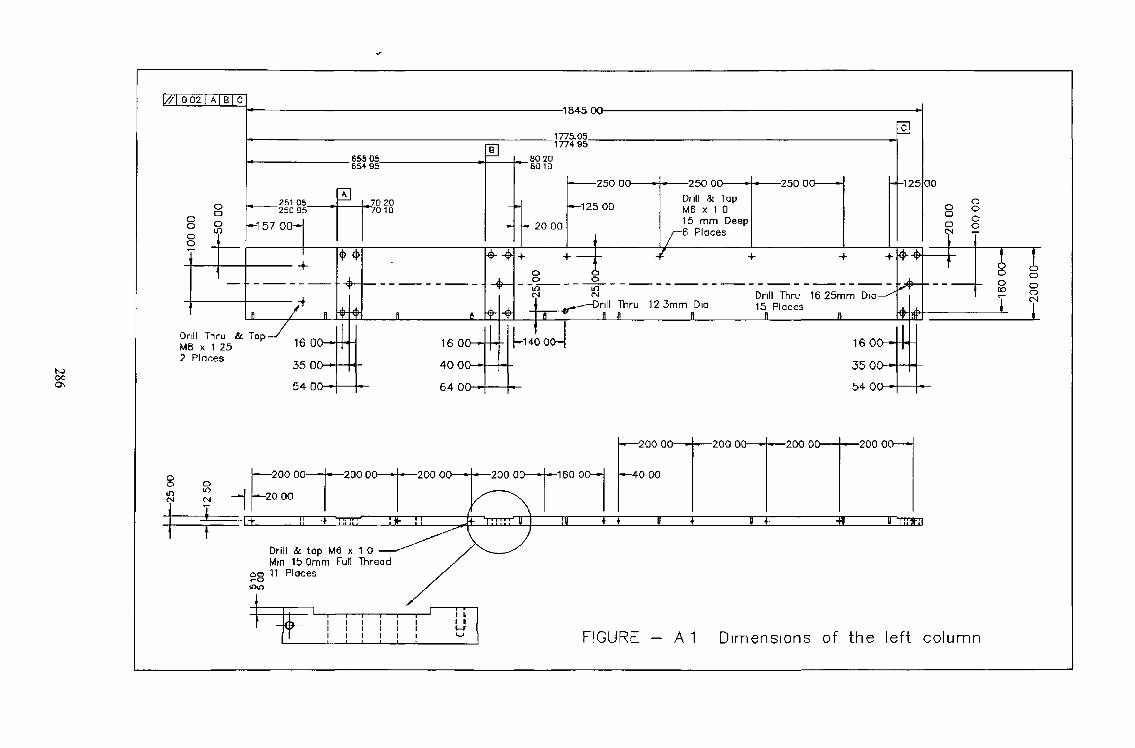
and also for easy dismantling Figure 3 3 shows the main frame, and figures A 1 and A 2 of
appendix A show detailed drawings of the columns There are no differences between the
back and front columns except that more holes were drilled in the back columns to fix the
motor's frame to the main structure of the machine
The bottom plate holds the torsion shaft with the help of a pair of cylindrical roller bearings
The lower end of each ball screw rests in this plate by a pair of taper roller bearing Details of
the bottom plate are shown in figuie 3 4
27
The drive shaft housing holds the torque-tension shaft and the lower end of each guide rod A
pair of taper roller hearings was used to fix tins shaft in the housing Details of the housing are
shown in figure 3 5 The top plate holds the other ends of the ball screws and guide rods This
plate contains a specially designed feature (details of which is given under the heading
"preloading unit") for applying the necessary pre-load to the bearings which are fitted with the
ball screws It has also provisions for fixing necessary auxiliary components (1 e , gnpper
and/or holder) so that simple compression tests could be earned out by placing specimens in
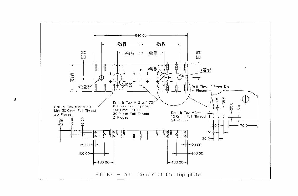
between this plate and the movable cross head Figure 3 6 shows the dimensions of the top
plate in detail
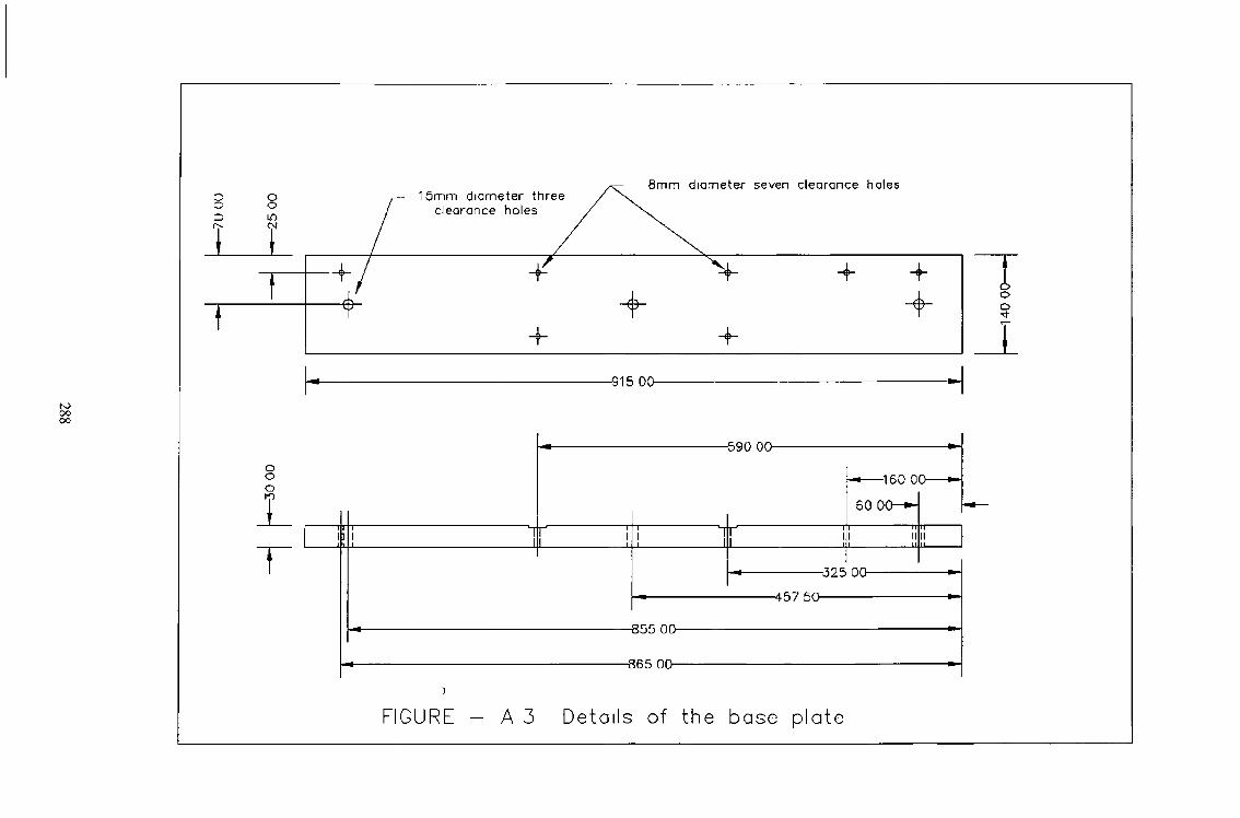
The entire machine, along with its drive systems, rests on two base plates which sit on six
levelling pads The base plates were screwed to the four columns using a set of M5xl 5
socket head cap screws Details of the base plate are shown in figure A 3 of appendix A
3.2.2 MOVING PARTS AND RELATED COMPONENTS
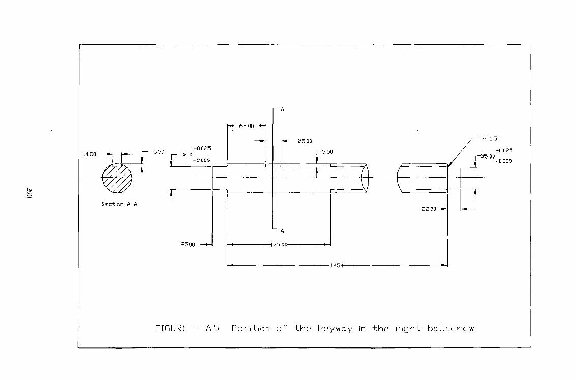
(0 BALL SCREW
Two induction hardened ball screws, 1454mm long, 50mm m diameter and 10mm pitch thread
were used to dnve the cross head and apply the necessary axial load to the specimen The
matenal of the ball screws is caibon steel, with an average carbon content of 0 45% and
average manganese content of 0 60% This steel confirms to Swedish and German standards
SS 1672 and DIN Ck 45 It is equivalent to steel type 3 in the ISO/R 638/1-1968 and ISO/R
683/XII-1971 international recommendations Both screws were purchased from "PGM
Ireland Ltd ", model number PG-050-10 Details specification regarding the screws are given
in table 3 2
The 140mm long nut of each ball screw was screwed into the cross-head so that it (cross
head) attains a linear vertical motion whenever the ball screws rotate These screws
28
experience only compressive forces The top and bottom ends of each ball screw were
attached to the top and bottom horizontal plates respectively, by a set of taper roller bearings
A specially designed feature was made at the top ends of each ball screw, fitted into the top
plate, to apply necessary pre-load to the above mentioned taper roller bearings Over the
unthreaded portion of each screw one steel timing pulley of 10mm pitch and 127 32 PCD has
been keyed to drive (them ball screws) using timing belts Details of the ball screw are shown\
in figure 3 7 Figures A 4 and A 5 (in appendix A) show the positions of the key way in the
unthreaded portion of the ball screws
Table -3 2 Details o f the ball screw
Pitch circle diameter 52 17 mm
Lead 10Ball diameter 6 35 mm
Dynamic rating 4331 daN
Static rating 10041 daNNut spring rating 1954 N/jim
Hardness 180-225 (HB)
Yield point 370 N/mm2
Tensile strength 620-760 N/mm2Hardness after induction hardening 57-63 (HRC)
Diameter tolerance h8
Straightness 0 2 (mm/m)
(u) GUIDE ROD
Two steel shafts, 1040mm long and 50mm in diameter, were chosen as guide rods When
torque is applied to the test specimen through the torque-tension shaft, the cross head, and
hence the ball screws, also expenence the same torque from the resulting twisting moment
Thus the guide rods were used to prevent the ball screws from experiencing the bending
forces which develop due to tins twisting moment The guide rods were designed in such a
29
way that they can withstand the resulting bending moments and thus the ball screws
experience only axial load during the simultaneous application of torque and tension
The top and bottom ends of each guide rod were fitted into the slots provided in the top and
bottom plate of the machine respectively The end faces of the rods were screwed into these
plates to assure rigidity of the machine Details of the guide rods are shown in figure A 6
The average chemical composition of these induction hardened steel shafts is as follows C
square drive, thin plates, and all components of the pie-loading units
HEAT-TREATMENT
All the components manufactuied from the "Orvar Supreme" steel were heat-treated
according to the following procedure to obtain haidness of between 52-54 HRC
Preheating
1st preheat to 650 deg C
2nd preheat to 850 deg C
Soaking
Soaked (Austemzed) at 1040 deg C for approx 40mins
Quenched to 50 deg C under 3 bar pressure of mtiogen
Tempering
Tempered twice at 200 deg C for two hours, cooling to room temperature each time
64
3.8 DESIGN EQUATIONS
STRESSES UNDER STATIC AND DYNAMIC CONDITION
Following equations, where appropriate, were used in designing various parts of the torque-
tension machine For a biaxial stress state induced by a normal stress a and a shear stress x on
a particular plane, the design equation based on octahedral shear stress theory and for static
loading, can be written as
where Y and t y are the yield stress in tension and in shear respectively, n is the design factor
based on yield strength For octahedral shear stress theory, Ty = Y / V3 For combined
bending and uniform axial stresses, the normal stress a can be expressed as
and due to the torque T, the resulting shear stress t = Tc / J, where J is the polar second
moment of an area
For varying normal and shear stresses on a plane at a point, the design equation, based on
octahedral shear stress theory, is
where Gme and CTa are the mean and the alternating component of the stress 0 en is the
endurance limit at critical location of machine element and k f the stress concentration factor
RIGIDITY
Rigidity is high stiffness and low deflection, in either or both the lateral and torsional
directions High rigidity is desirable because it produces a high natural frequency, maintains
65
gear contact, maintains uniform oil film in gears and beanngs, and improves the performance
accuracy of the machine
A torque produces an angular deflection Geneially angular rigidity is expressed as angular
deflection per unit length of the shaft, 1 e , degree/unit length Angular rigidity in terms of
torque, shear modulus of rigidity and polar moment of area is
6 180T ^— = ------- (deg /unit length)L kGJ
where T is m inch-lbf
Lateral loads produce lateral deflections which vary along the shaft depending on the type of
loading and the geometric properties of the shaft Lateral deflection can be calculated using
either integration or area moment method as used m case of beams
TORQUE REQUIRED TO TURN THE BALL SCREW
Motion in a direction opposite to the direction of the applied load involves a torque T and a
axial load F which are related by the equation
FD FDT = ■ tan(p + *-)■+
where JLXC = collar fnction, D p and Dc are the screw pitch and collar mean diameter
respectively The parameter p is a thread-fnction paiameter and X is the lead angle
BUCKLING FORMULA
Euler's design equation for slender column can be written as
F = k2E A _ n ( ^ / K )2
where C, is the end condition factor in buckling and ¿7 k is the slenderness ratio The Euler
equation is applicable only when the £ / k ratio is large, that is, when
66
For smaller £ / k ratios, the J B Johnson or parabolic formula should be used, which can be
wntten as
In order to calculate the stiffness of the toique-tension machine an analytical model has been
developed and presented in this section For simplification of calculations the complex
structure of the machine has been resolved into elements and represented as two dimensional
beams as shown in figure 3 29(a) The mathematical model of the machine was studied using
simple bending theory based on total strain eneigy principle However, dunng modelling only
the axial load and the resulting bending moments have been considered The effect of twisting
moment due to the applied torque has been excluded from tins model To simplify the model,
various auxiliary parts, such as steeped shaft, holders, gnppers etc, which are not involved in
building the mam structure of the machine, have also been excluded
In developing the model, it was necessary to make the following assumptions
(1) The beams are in 2D and aie initially straight and unstressed
(n) The material of the beams is perfectly homogeneous
(in) The elastic limit is nowhere exceeded
( i v ) Neutral axis passes through the centroid of the cross-sections
(v) The weight of the machine and friction forces are negligible
(vi) The applied load is symmetrically static and shared equally by the front and the back
columns of the machine
3.9 STIFFNESS OF THE MACHINE
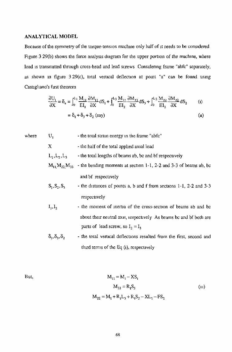
ANALYTICAL MODEL
Because of the symmetry of the torque-tension machine only half of it needs to be considered
Figure 3 29(b) shows the force analysis diagram for the upper portion of the machine, where
load is transmitted through cross-head and lead screws Considering frame "abfc" separately,
as shown in figure 3 29(c), total vertical deflection at point "a" can be found using
Castigliano's first theorem
rL3 M ^ 9M330 e i2 T x "
dS3 + J= + 83 + 82 (say) (u)
where U - the total strain energy in the frame "abfc"
XX - the half of the total applied axial load
Lj ,L2 ,L3 - the total lengths of beams ab, be and bf respectively
Mn M22M33 - the bending moments at section 1-1, 2-2 and 3-3 of beams ab, be
andbf respectively
S1,S2, S3 - the distances of points a, b and f from sections 1-1, 2-2 and 3-3
respectively
- the moment of inertia of the cross-section of beams ab and be
about their neutral axis, lespectively As beams be and bf both are
parts of lead screw, so I2 = I3
8i,53,82 - the total vertical deflections resulted from the first, second and'1* 3 »u2
third terms of the Eq (1), respectively
But, Mn = Mj -XS;
M33 - R-1S3 (m)
M22 — Mj + RjL3 + — XLj — FS2
68
where, - the unknown redundancy bending moment at point a
F - the unknown force at point a
Rj - the unknown reaction force at point f
Differentiating equations (111) with respect to X and substituting the corresponding values in
equation (1), becomes
5 L' [XL! M, 1 “ Eli L 3 2
8,=0
S2 = {¿XL, + FL2 - 2M, - Rj(2L3 + L2)}2 EL
(iv)
(V )
(V I)
The unknown values of R,, M] and F can be found from the relations
dU,9Rj
- 0 andau,aivi,
But _ fLl M , , ^ M , , c| r + |*L3 m 31 3 m 3,
0R, El, 3R, 1 Jo EI2 9R, dS3+ J0l2 M „ 3M
dS (vu)EI2 dR{
= 8 + 5 + 5 (say)
Differentiating equations (111) with respect to Rj and substituting the corresponding values in
Eq (vu), gives
5 =0
8 =_ R,U3EL
5” = -X L,L2fL 3 + M,L2Î l 3 +%- ] + R,L.
But as 8 + 8 +8 = 0 ,so from the above equations,
T2 ^L3 + L2L3 +
v / 21 2 3
where
R _ XL,L2Q M,L2Q | FL22(L3 /2 + L2 / 3) 1 Z Z Z
Q = (L3 + L2/2 )
(vrn)
(ix)
69
and Z = L33 / 3 + L 2L23 + L22L 3 + L32 / 3 (x)
Taking moment at point c, as ^ Mc = 0,
so Rj(L2 + L3) + M !-X L ,-F L 2 = 0 (xi)
3UAgain, according to the Castigliano's second theorem, = 0 (xn)
oMj
which can be written as
= fLl M li.M lijs + f' 3 ,M„ 9M „ dS ft-2 M22 3M22 dS9m, jo EIX 3M, 1 Jo EI2 3Mj 3 Jo EI2 3M,
Using equations (111) and (xn), and after simplification, Eq (xm) provides
+ I2L2) - X + r , i 2 L 2L 3 + Y - n 2 Y = 0 (XIV)
where, for simplification, 1/I j and 1/ I 2 have been replaced by Ij and I2 respectively
Now substituting Eq (vm) into (xi), after simplification, becomes
F = M1D -X W (xv)
where D = B/C and W = A/C, in which,
- L i
g _ + L 3) i
z
and c = La2( 3L , ->2 L ,)(L ; + L j) _6Z 2
Now, substituting the values of Rj, from Eq (vm), and F, from (xv), into Eq (xiv) gives
JM1= X - (xvi)
where
and K = ^Lj + 12 ^2DU L22 ^
L 2L 3 + h i (3 l , + 2 u - q h
Thus knowing the values of M1? F and Rp from equations (xvi), (xv) and (vrn) respectively,
the values of 5t and 52 of equations ( i v ) and (vi) can be found
Figure 3 30(a) shows the free body diagram of the beam "de" Total vertical deflection at
point c, due to transmitted axial load through lead screw, can be obtained as follows
t)U2 _ s _ fL5 M „ 3M55 rL4 M44 3M44ax EIS 9X
dS + r5 Jo FT.ei4 ax
dS, (xvn)
where U2 - the total strain energy in the beam "de"
L4, L5 - the distances between the points c-e and c-d respectively
M44,M 55 - the bending moments at section 4-4 and 5-5, respectively
The unknown redundancy moment M3 can be obtained by taking moment at point d Thus
M3 = XL5 As
m 44 = m 3 = x l 5
and
so equation (xvii) becomes
M55=M 3-X S 5
5 =_ X U 5
ELL l + L3 Lr
(xviu)
However, deflection of beam "dk" can be found considering it as a short compression block
Thus
EA<(xix)
where L6 and A6 are the length and cross-section of the beam ndk"
71
Figure 3 30(b) shows the force analysis diagram for the lower portion of the machine, where
the load is transmitted through drive shaft housing and vertical columns The vertical
displacement at point b can be found as follows
3U3 _ fL7 M77 3M77 rLs M „ dU,- g - f 77 q iV 177. d S 88 W 1 88 ¿ o / x
°b - Jo F T . S X db7+Jo FT. di>8 (XX)ax D J° e i 7 ax Jo e i8 ax
=57+sg (say)
As M2 = XL7 (taking moment at point m), M77 = -M 2 +XS7, and M88 = XL7 - M 2 + F2S8,
so "
57 = - ^ - (xxO7 6EI, 1
2
(xxu)2EIo
The value of unknown redundancy force F2 can be obtained from the relation
So, F2 = X ^-h VL8
Thus after knowing the values of 8j, 82, 8C, 5d and 8b, from equations ( i v ) , (vi), (xviu), (xix)
and (xx) respectively, the stiffness of the machine can be obtained for the design load
72
FIGURE — 3.1 Schem atic diagram of the m achine (Front view) (M otors and fram es are not shown in the figure)
FIGURE - 3 2 S ch em a tic d iag ram o f t h e nachm e (Side view) (Guide r o d s and ba ll s c r e w s a r e n o t shown in t h e f i g u r e )
FIGURE - 3 3 The schematic diagram of the main frame of the torque-tension machine
( The bolts and the drilled holes are not shown in the figure)
75
32
00
Drill * Top M6 x 1 0 ~ 1100 PCD
Drill & Tap M16 x 2 0 Min 3 0 0m m Full Thread 2 0 Places
O CD ooro tO r<£>
Drill & Tap Ml 2 x 1 75 6 Holes Equi Spaced 1 4 0 0m m P C D 3 0 0 Mm Full Thread 3 P laces
♦ L IIHi> i1
f 11 !1 '1 1
«i♦4-4- i
20 00 -
100 00-
-180 00—
-20 00
-100 00
—180 00—
FIGURE — 3 6 Details of the top p late
1
(200) 1476 STANDARD LENGTH FULL TRACK
140
St). 025| A
u r_ j — '— ■—h -1— =>uf ! r r rb r r r r r tr^ r r t= r= 3r rk r 3=rri3 [
74. 990 74.971 (q6)
IQItO. 025[Äl flEG ISIEB
<874. 5
OIL POINTJLJdQULDBILLJLIAE 1ZS^B^L^_X _12_DEEE ÛBILU P 4 TBELCL
45,0ROOT DIA
i!ÏLOfLBRUSH_WIPEB EACH _ENQ
ÊJdQ L£S_O B IU LJLll_ IH 0 (L.CZBQHEJ>JL8_X_10J_D£EE£BUI=SEACEtUWLAJiL£JLJDIA
FIGURE - 3 7 Details of the ballscrew
II
b i n
■m—|--------r
“T"- L
T nr
n— r - v i
5 1 0 -
ri'n
MISm i n 3 0 F u L L -fc to t— e - a o< *4- place
nji iLr|i ^Llin
fi
FIG URE - 3 .8 D e t a i l s o f t h e c r o s s - h e a d
Top thin p la te
B o t t o n -thin p la t e
Steeped s h a f t
FIGURE - 3 9 The c o m p le te c r o s s - h e ad a r r a n g e m e n t inc lud ing t h e dowel pin, load c e l l and o t h e r a u x i l i a r y co m p o n e n ts
Holder
FIGURE — 3 10 Assembly drawing of the to rque—tension shaft along with the taper roller bearings and other accessories
FIGURE — 3.12 Geometry of the specimen holder
N u t l Nu t2
A d j u s t e r
T op p la te
Ball s c re w
FIGURE - 314 Assembly drawing o f t h e p re load ing un i t
•Other Controllers
LI
L2 1
L3 «
PE
Matching transformer
♦Power Supply
Controller (rating Ic)
Brushtess Servomotor
Mams
Command signal
FIGURE - 3 15 The schematic diagram of a Moog brushless drive system
H T = Yield torque□ T = 75% of Y torque0 T = 50% of Y torqueA T = 25% of Y torque
N o r m a l i s e d ax ia l l oad
F i g u r e 6 . 5 N o r m a l i s e d t o r q u e v e r s u s n o r m a l i s e d a x i a l l o a d c u r v e ( a n g l e o f t w i s t c o n s t a n t )
Steel1 25
1 00
0 75
0 50
0 25
0 00
a Torque o Axial load
! i i i i i i i i i i i i i i i i i i i i i i i i i i \ i i i \ i i r
0 00 0 50 1 00 1 50 2 00 2 50 3.00 3.50
N o r m a l i s e d ax ia l s t r a i n
Figure 6 6(a) Normalised axial strain versus normalised torque and load curves(T ■ yield torque)
Steel
N o r m a l i s e d ax ia l s t r a in
¿ Axial load o Torque
F i g u r e 6 . 6 ( b ) N o r m a l i s e d a x i a l s t r a i n v e r s u s n o r m a l i s e d t o r q u e a n d l o a d( T = 7 5 % o f y i e l d t o r q u e )
Steel
N o r m a l i s e d a x i a l s t r a i n
* Axial load o Torque
Figure 6.6(c) Normalised axial strain versus normlised torque and load(T = 50% of yield torque)
Copper
1 00
0 75
0 50
0 25
0 0 0 i i i i | i i i i | i i i i | i i i i | i i i i
0 00 0 25 0 50 0 75 1 00 1 25
N o r m a l i s e d a x i a l l oad
D O D D
0 0 0 0 0 0
A & A A
0
A A A
■ T - Yield torque□ T - 75% of Y torque0 T - 50% of Y torqueA T = 25% of Y torque
F i g u r e 6 7 N o r m a l i s e d t o r q u e v e r s u s n o r m a l i s e d a x i a l l o a d c u r v e ( a n g l e o f t w i s t c o n s t a n t )
Copper
N o r m a l i s e d a x i a l s t r a i n
o Nor torque * Nor axial load
Figure 6.8(a) Normalised axial strain versus normalised torque and load curve(T = yield torque)
Copper
N o r m a l i s e d ax i a l s t r a i n
o Nor torque ¿ Nor axial load
Figure 6 8(b) Normalised axial strain versus normalised torque and load curve(T - 75% of yield torque)
Copper
N o r m a l i s e d a x i a l s t r a i n
Figure 6.8(c) Normalised axial strain versus normalised torque and load(T = 50% of yield torque)
Nor
mal
ised
sh
ear
stra
in
Steel4.50
4 00
3 50
3.00
2 50
2 00
1 50
1 00
0.50
0 0 0 i i i i | i i i i | i i i i | i i i i | i i i i | i i i i | i i i i | i i i i | i i i i
0 00 0.50 1 00 1 50 2 00 2 50 3 00 3 50 4.00 4 50
N o r m a l i s e d ax ia l s t r a i n
yield torque 75% of Y. torque 50% of Y. torque 25% of Y torque
0 F = Yield load□ F = 75% Of Y loado F = 50 % of Y loada F = 25% of Y load
N o r m a l i s e d t o rq u e
F i g u r e 6 . 1 0 N o r m a l i s e d a x i a l l o a d v e r s u s n o r m a l i s e d t o r q u e c u r v e ( a x i a l d i s p l a c e m e n t c o n s t a n t )
Steel
N o r m a l i s e d shear s t r a i n
Figure 6.11(a) Normalised shear strain versus normalised axial load and torque curves(F = yield load)
Steel
N o r m a l i s e d shear s t r a i n
Figure 6.11(b) Normalised shear strain versus normalised axial load and torque curves(F - 75% of yield load)
Steel
N o r m a l i s e d shear s t r a i n
Figure 6.11(c) Normalised shear strain versus normalised axial load and torque curves(F = 50% of yield load)
Steel
N o r m a l i s e d shear s t r a i n
*■ Torque o Axial load
Figure 6 11(d) Normalised shear strain versus normalised axial load and torque curves(F = 25% of yield load)
Copper
1 00
0 75
0 50
0 25
0.00
B F = Yield load□ F = 75% of Y load0 F = 50% of Y load& F = 25% of Y load
N o r m a l i s e d t o r q u e
Figure 6.12 N o r m a l i s e d a x i a l l o a d v e r s u s n o r m a l i s e d t o r q u e c u r v e ( a x i a l d i s p l a c e m e n t c o n s t a n t )
Copper
N o r m a l i s e d shear s t r a i n
Figure 6 13(a) Normalised shear strain versus normalised axial load and torque curve(F = Yield load)
Copper
N o r m a l i s e d shear s t r a i n
a Nor torque o Nor axial load
Figure 6.13(b) Normalised shear strain versus normalised axial load and torque curve(F = 75% of yield load)
1.50Copper
1 25 —
1 00
0 75
0 50
0 25
0 00
A A A A
0 0 0o 0 0 0 0
A A A a Nor torque o Nor axial load
1 i i I | I I ! I I I i i I I I I 1 I I I I I I I I I I I I I I ! r
0.00 0 50 1 00 1 50 2 00 2 50 3 00 3 50
N o r m a l i s e d shear s t r a i n
Figure 6.13(c) Normalised shear strain versus normalised axial load and torque curve(F ■ 50% of yield load)
1 500
1 250
1 000
0 750
0 500
0 250
0 000
0 00 0 50 1 00 1 50 2 00 2 50 3 00 3 50
N o r m a l i s e d shear s t r a i n
Copper
* Nor torque o Nor axial load
ure 6.13(d) Normalised shear strain versus normalised axial load and torque curve(F = 25% of yield load)
Nor
mal
ised
ax
ial
stra
in4.50
4.00 —
3 50 - 5
3.00
2.50 - 3
2 00
1 50
1.00
0.50
0.00
Steel
- ? D—n À3> o
i
0 00
B
□ □▲ ▲0 0 i—i—i—i—r
0 50
▲
0i—i—r i— i—r
0
i—i—r i—i—i—i—i—i—r
■ F - Yield load□ F n en sP 0s of Y loadA F » 50% of Y load0 F - 25% of Y load
1.00 1 50 2.00
N o r m a l i s e d shear s t r a in
2 50 3 00 3.50
F i g u r e 6 . 1 4 N o r m a l i s e d a x i a l s t r a i n v e r s u s n o r m a l i s e d s h e a r s t r a i n c u r v e ( f o r c e m a i n t a i n e d c o n s t a n t )
Shea
r st
ress
(N
/mm
2
)
* T - Yield torque a T - 75% of Y torque & T » 50% of Y torque
A x ia l s t r e s s ( N / m m 2 J
Figure 6.15 Determination of yield points due to combined loading(angle of tw ist constant)
Copper
A x ia l s t r e s s ( N / m m 2)
Figure 6 16 Determination of yield points due to combined loading(angle of twist constant)
Axi
al
stre
ss
(N/m
m2
)Steel
♦ F - Yield load□ F - 75% of Y load<r"F - 50% of Y loadA F - 25% of Y load
Shear s t r e s s ( N / m m 2 )
Figure 6.17 Determination of yield points due to combined loading(axial displacement constant)
Copper300
250
200
150
100
50
Yield locus based on proof stress
B Axi al st ress ( F0 Axi al st ress ( FD Axi al st ress ( FA Axi al st ress ( F
Y load ) 75% of Y L) 50% of Y L 25% of Y L
Yield loci based on post-yteld flow stress
Shear s t r e s s ( N / m m 2 )
Figure 6.18 Determination of yield points due to combined loading(axial displacement constant)
Nor
mal
ised
sh
ear
stre
ss
Steel
N o r m a l i s e d ax i a l s t r e s s
F i g u r e 6 1 9 ( a ) C o m p a r i s o n o f e x p e r i m e n t a l l y o b t a i n e d y i e l d s t r e s s e s w i t h t h o s e o fM i s e s ' a n d T r e s c a ' s
Nor
mal
ised
sh
ear
stre
ssCopper
N o r m a l i s e d a x i a l s t r e s s
F i g u r e 6 . 1 9 ( b ) C o m p a r i s i o n o f e x p e r i m e n t a l l y o b t a i n e d y i e l d s t r e s s e s w i t h t h o s e o fM i s e s ' a n d T r e s c a ' s
Specimen - 1
CVJIo
X a>CJ-o
■ S G - 1o S G - 2a S G ■ 3□ Torque transducer
A x ia l s t r a i n ( m i c r o - s t r a i n )
Figure 6 20(a) Varit ions of the torque and shear strain gauges' readings with axialstrain (uniform diameter specimen)
Shea
r st
rain
(m
icro
-str
ain
)
Specimen - 211000
10000
9000
8000
7000
6000
5000
4000
3000
2000
1000
0
■ S G - Io S G - 2* S G - 3a Torque transducer
A x ia l s t r a i n ( m i c r o - s t r a i n )
Figure 6.20(b) Variations of torque and shear strain gauges' readings with axial strain(uniform diameter specimen)
Specimen - 3
toto00
c5
Co1"s O
1 o
c\î~1o c:
XTOv«.■*—.
q>=3
co
O' (0CD
o -cK. Co
■ S G - 1o S G - 2a S G - 3s Torque transducer
t i— i i | i i i i ¡ i— i— i— i— |— i— i i i | m — i— i— |— i i i i |— i i— i— i— |— i i i— r |
0 500 1000 1500 2000 2500 3000 3500 4000
A x ia l s t r a i n ( m i c r o - s t r a i n )
Figure 6.20(c) Variations of torque and shear strain gauges' readings with axial strain(uniform diameter specimen)
Specimen - 4
totoVO
CMtO
XQ)=3t ro y—
c<5>*-*CO
■oo
c5
CO
»>-COQ>■c:CO
■ S G - 1o S G - 2a S G - 3a Torque transducer
A x ia l s t r a i n ( m i c r o - s t r a i n )
Figure 6.20(d) Variations of torque and shear strain gauges' readings with axial strain(uniform diameter specimen)
She
ar
stra
in
(mic
ro-s
tra
in)
8000
6000
4000
2000
0 i i i i | i i i i | i i i
0 500 1000 1500 2000 2500 3000 3500 4000
A x ia l s t r a i n ( m i c r o - s t r a i n )
A A
-o □ □ □
A A A
□ □ □ □ □ Q □□ □ □
® S G -1 A S G -2 O S G -3□ Torque transducer
Figure 6.21(a) Variations of torque and strain gauges' readings with the axial strain(reduced section specimen)
c:
^ £
CO
><
CO
><
CoIoo
c(5
■+-*CO
TOa>-c:CO
12000
10000
8000
6000
4000
2000
® S G -1 ■ S G -2 o S G -3 - Axial load cell
i — i— i |— i— i— i— i— i— i— i— |— i i— i— i— i— i— i— |— i— i— i i— i— i— i— |— i— i— i— i— i— i— r
2000 4000 6000 8000 10000
Shear s t r a i n ( m i c r o - s t r a i n )
Figure 6.21(b) Variations of axial load and strain gauges' readings with the shear strain(reduced section specimen)
Nor
mal
ised
ax
ial
loa
d
Steel1 50
1 25
1 00
0 75
0 50
0 25
0 00
m
P
dOO . 0
0 Oe
— 0 75
a 0 0
o Nor axial load * Nor torque
1 00
— 0.50
0 25
0. 00
Time (sec )
Figure 6.22(a) Variations of normalised torque and axial load with time(init ia l T - 98% of yield torque)
Nor
mal
ised
to
rqu
e
Steel
Time (sec )
Figure 6.22(b) Variations of normalised torque and axial load with time(initial T = 75% of yield torque)
Steel1 25
1 00 -
0 75 —
O 50
O 25
o °>o
o °o o 0o o
A A A A A A
OA A A
aA A A *A * A A /
Oo
o Ñor axial load ± Ñor torque
0 00 —i T I I I 1 I I I 1 I I I I I I I I I I
20 40 60 80 100 120 140
Time (sec )
Figure 6.22(c) Variations of normalised torque and axial load with time(init ia l T - 50% of yield torque)
Nor
mal
ised
to
rqu
e
Copper1 25 1 50
1 00
0.75
0 50 —
0
0 00
1 25
1.00
0 75
0 25 0.50
0 00 —
-0 25 i i i
10
0
T20
i—i—r i i l i
¿ Nor torque o Nor axial load
i—i—r
0 25
0 00
30 40 50 60 70
Time (sec )
Figure 6.23(a) Variations of normalised torque and axial load with time(init ial T = yield torque)
Nor
mal
ised
ax
ial
loa
d
Nor
mal
ised
to
rqu
e
C opper1 50 1 25
1.25
A Nor torque o Nor axial load
0
0 0 0
1 00
1 00° o „ 0
0 — 0 75
0 75 — s, A A A A — 0.50
0 50 0 25
0 25 0. 00
Time (sec )
Figure 6.23(b) Variations of normalised torque and axial load with time(init ia l T = 75% of yield torque)
Nor
mal
ised
ax
ial
loa
d
Copper1 25
1 oo
0 75
0 50
0 25
O 00
Figure 6.23(c) Variations of normalised torque and axial load with time(init ia l T = 50% of yield torque)
* Nor torque o Nor axial load
0
0
y i i~r i | i i n | i i r i | i i i i | i i i i | i i i i | i i i i | i i i i | i i i i | i i i i | i i i" i [ ~n
0 10 20 30 40 50 60 70 80 90 100 110
Time (sec )
Nor
mal
ised
ax
ial
loa
d
Steel1 75 1 50
1 50
1 25
0
0
0
1 25
1 00
1 00m
A A — 0 75
0 75 0 50
0 50
0 25
* Nor axial load o Nor torque
— 0 25
0 00
Time (sec )
Figure 6.24(a) Variations of normalised axial load and torque with time(init ia l F = yield load)
Nor
mal
ised
to
rqu
e
Steel1 75
1 50
1 25
1 00
0 75
0 50
0 25
0 00
0 20 40 60 80 100 120
Time (sec )
Figure 6 24(b) Variations of normalised axial load and torque with time(init ial F = 75% of yield load)
o Nor torque ¿ Nor axial load
0
A A0
A a
y — i— i— i— i— i— i— i— i— i i— i i i i— i i i r i— i— í— i— i— i— i— i— r
Steel1 75
1 50
1 25
1 00
0 75
0 50
0 25
0 00
Figure 6 24(c) Variat ions of normal ised axial load and torque wi th t ime( in i t i a l F = 50% of y ie ld load)
o Nor torque ¿ Nor axial load
0
0a A A A
0
Time (sec )
Steel1 75
1 50
1 25
1 00
0 75
0 50
0 25
0 00
Figure 6 24(d) Variations of normalised axial load and torque with time(intial F = 25% of yield load)
o Nor torque ¿ Nor axial load . 0 o 0 0 0 0 < > < >
„ 0 0 » 0 0 V o
£ A A A A á a a A A A A ^ A A A A A A A a
Time (sec )
Nor
mal
ised
to
rqu
e
Copper1 50 1 25
1 25
1 00
0 75
A A
0 0
1 00
0 75
0 50
0 50 - 0 25
0 25
0 00 — y i—i—i—i—|—i—i—i—i—|—i—i—i—r
0 10 20 30
o Nor torque a Nor. axial load
t—i—|—i—i—i—i—|—i—i—i—i—|—i—i—i—r—|—r
40 50 60 70
0 00
-0.25
Time (sec)
Figure 6 25(a) Variations of normalised axial load and torque with time(init ia l F ■ yield load)
Nor
mal
ised
ax
ial
loa
d
Copper1 DU
1 25
0 0 00 o
o oo
1 00
O 75O
A A
0.50
A
O 25
O 00
o Ñor torque a Ñor axial load
~ n
10
t—i—i—i—r
20 30 40 50
t—i—r t—i—:—r
60 70
Time (sec)
Figure 6 25(b) Variations of normalised axial load and torque with time(init ial F ■ 75% of yield load)
Copper
0 10 20 30 40 SO 60 70
Time (sec )
Figure 6.25(c) Variations of normalised axial load and torque with time(init ia l F - 50% of yield load)
1 50
1.25
1.00
0 75
0.50
0 25
0 00
Figure 6.25(d) Variations of normalised axial load and torque with time(init ia l F - 25% of yield load)
Copper
o Nor torque a Nor axial load
O 0 0
0
A A
•y— i— i— i— i— |— i— i— i— i— j— i— i— i— i— I— i i— i— i I— i i i— i |~ n i i i I i i i i I r
0 10 20 i 30 40 50 60 70
Time (sec)
Nor
mal
ised
to
rqu
eSteel
» T - Yield torquea T - 75% of Y torquea T - 50% of Y torque♦ T - 25% of Y torque
N o r m a l i s e d ax i a l s t r a i n
Figure 6.26 Comparison of experimental results with Gaydon's theoretical model(twist constant)
Nor
mal
ised
to
rqu
eSteel
■ T - Yield torqueo T - 75% of Y torquea T ■ 50% of Y torque« T - 25% of Y torque
N o r m a l i s e d ax ia l s t r a i n
Figure 6 27(a) Comparision of experimental results with Gaydon's theoretica l model(twist constant)
Nor
mal
ised
to
rqu
eSteel
N o r m a l i s e d ax ia l s t r a i n
Figure 6.27(b) Comparison of experimental results with Gaydon's theoretical model(twist constant)
N o r m a l i s e d a x i a l s t r a i nFigure 6.28 Comparison of experimental result with Brooks' model
(angle of twist constant)
Copper
to
o
<D
&•
Q>y>15£
a T - Yield torque□ T - 75% of Y torque$ T - 50% of Y torque£ T - 25% of Y torque
N o r m a l i s e d ax ia l s t r a i n
Figure 6.29(a) Comparision of experimental results with Gaydon's theoret ica l model(twist constant)
Nor
mal
ised
to
rqu
eCopper
N o r m a l i s e d ax ia l s t r a i n
■ T - Yield torque° T - 75% of Y torque* T - 50% of Y torque- T - 25% of Y torque
Figure 6.29(b) Comparison of experimental results with Gaydon's theoret ica l model(twist constant)
Nor
mal
ised
ax
ial
loa
dSteel
» F □ Fo F a F
Yield load 75% Of Y 50 % of Y 25% of Y
N o r m a l i s e d shear s t r a i n
Figure 6.30 Comparison of experimental results with Gaydon's theoretical model(axial displacement constant)
loadload
load
Nor
mal
ised
ax
ial
loa
d
1.00
o 75
O 50
O 25
0 .00
F i g u r e 6 . 3 1
■ F - Yield toadQ F - 75% of Yo F - 50% of Ya F - 25% of Y
0.00 0.50 1.00 1 50 2 00 2 50 3 00 3.50
Copper
N o r m a l i s e d shear s t r a in
Comparison of experimental results with Gaydon's theoretical model(axial displacement constant)
loadloadload
Nor
mal
ised
ax
ial
loa
d
N o r m a l i s e d shear s t r a i n
Figure 6.32 Comparision of experimental results with Brooks' theoretica l model(axial displacement constant)
Nor
mal
ised
to
rqu
e1 oo
0 75
0 50
0 25
0 00
0 00 0 50 1.00 1 50 2 00 2 50 3 00
N o r m a l i s e d ax ia l s t r a i n
a Thin-walied tube o Solid steel a Solid copper
Figure 6.33 Comparision of thin-walled tube's results with those of solid steel and copper(angle of tw ist constant)
Figure 6 35(c) Variation of the applied axial load with the torque(load applied first)
Torque (N-m)
Figure 6 35(d) Variation of the applied axial load with the torque(load applied first)
258
Nor
mal
ised
to
rqu
eSteel
N o r m a l i s e d a x i a l l o a d
Figure 6.36 Subsequent ultimate yield locus (torque applied f irst)
No
rma
lise
d
torq
ue
Copper
B) Results from fig 6 35(b) (assuming fully plastic)
■ Ful ly s t ra in -h a rd e ne d* Ful ly p la s t ic
N o r m a l i s e d ax i a l l o ad
Figure 6.37 Subsequent ultimate yield locus (torque applied f irst)
Nor
mal
ised
ax
ial
loa
d
Steel
E Results from fig 6 35(c) (assuming fully plastic)
■ Ful ly s t ra in -h a rd e n e da Fu l ly p la s t ic
N o r m a l i s e d t o r q u e
Figure 6.38 Subsequent ult imate yield locus (axial load applied f irst)
Nor
mal
ised
ax
ial
loa
dCopper
B Results from fig 6 35(d) (assuming fully plastic)
■ Ful ly s t ra in -h a rd e ne da Ful ly p las t ic
N o r m a l i s e d t o r q u e
Figure 6.39 Subsequent ult imate yield locus (axial load applied f irs t)
Nor
mal
ised
ax
ial
loa
d
Steel
" Torque app l ied f i r s t* Load app l ied f i r s t
N o r m a l i s e d t o r q u e
F i g u r e 6 . 4 0 ( a ) C o m p a r i s o n o f s u b s e q u e n t u l t i m a t e y i e l d l o c i f o r t w o d i f f e r e n tl o a d i n g p a t h s
Nor
mal
ised
ax
ial
loa
d
Steel
N o r m a l i s e d t o rq u e
F i g u r e 6 . 4 0 ( b ) C o m p a r i s o n o f s u b s e q u e n t u l t i m a t e y i e l d l o c i f o r t w od i f f e r e n t l o a d i n g p a t h s
Torque appl ied f i r s tLoad app l ied f i r s t
Nor
mal
ised
ax
ial
loa
d
Copper
■ Torque app l ied f i r s t* Load app l ied f i r s t
N o r m a l i s e d t o r q u e
F i g u r e 6 . 4 1 ( a ) C o m p a r i s o n o f s u b s e q u e n t u l t i m a t e y i e l d l o c i f o r t w o d i f f e r e n tl o a d i n g p a t h s
Nor
mal
ised
ax
ial
loa
d
Copper
» Torque app l ied f i rs ta Load appl ied f i r s t
N o r m a l i s e d t o rq u e
F i g u r e 6 . 4 1 ( b ) C o m p a r i s o n o f s u b s e q u e n t u l t i m a t e y i e l d l o c i f o r t w o d i f f e r e n tl o a d i n g p a t h s
CHAPTER SEVEN
CONCLUSIONS
7.1 INTRODUCTION
This chapter provides a brief summary of the conclusions of the present thesis It is divided
into three main sections the first gives the summary of the general conclusions obtained
dunng the experimental investigation, the second provides the gist of this thesis contribution
and the third recommends suggestions for the future work
7.2 GENERAL CONCLUSIONS
The conclusions resulting from the current experimental investigation are summarised below
under the appropriate headings
Torsion Followed By Tension - Angle of Twist Constant
(i) In the first case, where the rod was initially subjected to a torque and then, keeping the
angle of twist constant, to a gradually increasing axial load, the increase in the axial load
resulted in decrease in the initially applied torque according to the yield criteria
(n) The initially applied torque started to decrease with the axial load only when the
combined stress of the material reached approximately the uniaxial yield stress of the material
(111) The increase in the axial load and hence the increase in the corresponding normal
stress developed faster than the decrease in the torque and the corresponding shear stress
( i v ) With a gradually increasing axial load, the rod behaved as if its torque carrying ability
was drastically reduced without in any way affecting its axial load carrying ability
267
(v) Dunng this biaxial loading, though the material yielded due to the combined loading
well before the applied axial load caused yielding on its own, all the axial load curves followed
elastic path
(vi) The higher the magnitude of the initially applied torque, the greater is the rate of
decrease of the torque with the increasing axial load
Torsion Followed By Tension - Torque Maintained Constant
(1) When the rod was initially subjected to a torque and then, maintaining the torque
constant, to a gradually increasing load ( and hence to a gradually increasing axial strain), the
shear strain started to increase rapidly only when the rod yielded due to the combined loading
(n) The higher the values of the initially applied torque, the higher is the rate of increase of
the shear strain with the increasing axial strain
Tension Followed By Torsion - Axial Displacement Constant
(1) In the third case, where the axial load was applied first, increase in the torque resulted
in decrease in the initially applied load according to the yield criteria
(n) The initially applied load started to decrease with the torque only when the combined
stress of the material reached approximately the uniaxial yield stress
(m) The increase in the torque and hence the increase in the corresponding shear stress
developed faster than the decrease in the axial load and the corresponding normal stress
( i v ) With a gradually increasing torque, the rod behaved as if its axial load carrying ability
was drastically reduced without in any way affecting its torque carrying ability
(v) Dunng this particular loading, though the material yielded due to the combined
loading well before the applied torque caused yielding on its own, all the torque curves
followed elastic path
(vi) The higher the magnitudes of the initially applied load, the greater is the rate of
decrease of these loads with the torque
268
(vu) The percentage reduction in the initially applied load due to the applied torque was
much lower than the percentage of reduction in the initially applied torque due to applied load
(as was observed in the first case) under similar biaxial loading conditions
Tension Followed By Torsion - Axial Load Maintained Constant
(I) In the forth case, where the rod was subjected to an initial load and then, maintaining
the load constant, to a gradually increasing torque (hence to a gradually increasing shear
strain), the axial strain started to increase rapidly only when the rod yielded due to the
combined loading
(II) The higher the values of the initially applied load, the greater is the rate of increase of
the axial strain with the shear strain
Combined Loading With The Reduced Section Specimen
(1) Test results with the reduced section specimen showed that, even though the angle of
twist of the specimen was held constant after applying an initial torque, the shear strain
increases very rapidly (with the axial strain) at the confined zone where the localised yielding,
and hence the plastic deformation begins The shear strain decreases at any other locations
(unloading) thus suggesting that plastic deformation in a uniform cross-section specimen takes
place at a certain preferred location with unloading taking place elsewhere
(u) In the second test it has been observed that even though the axial displacement of the
specimen was kept constant after applying an initial load, the axial strain increases very rapidly
(with the shear strain) at the confined zone where the localised yielding and hence the plastic
deformation begins The axial strain decreases at any other locations, hence, confirming that
plastic deformation takes place in a uniform cross-section specimen within a localised region
with unloading taking place elsewhere
269
Successively Applied Torque And Tension - Torque Applied First
(I) When the rod was initially subjected to an initial torque and then to successively
applied load and torque, keeping the axial displacement or the angle of twist constant
respectively in an alternate manner, the rod soon regains its axial load carrying capability
irrespective of the level of the initially applied torque
(II) With the successive application of the axial load and the torque, and when the material
yielded due to the combined loading, the increment in the axial load results reduction in the
torque and the increment in the torque results reduction in the axial load, 1 e , the effect of the
axial load or the torque whichever was applied subsequendy, was dominant on the specimen
investigated
(m) For the same type of loading as mentioned in (1), the influence of the axial load was
much stronger on the specimen investigated than that of the initially applied torque; as in this
case the subsequently applied torque resulted only in small reduction in the axial load
compared to the total amount of load applied
( i v ) The more the axial load was subsequently increased towards the yield and hence,
towards the ultimate load of the material, the less the percentage of reduction in the axial load
for the same amount of torque increment and also, the less amount of axial load was required
to cause the same drop in the torque
Successively Applied Torque And Tension - Load Applied First
(I) When the rod was initially subjected to an initial load and then to successively applied
torque and load, keeping the angle of twist or axial displacement constant in an alternate
manner, the rod soon regains its torque carrying capability irrespective of the initially applied
load
(II) The influence of the torque (which was applied as a second parameter) was much
stronger on the specimen investigated than that of the initially applied load, as the
subsequently applied axial load resulted only small reduction in the torque compared to the
total torque applied
270
Comparison Between The Experimental And The Theoretical Results
(1) For the biaxial loading, where the rod was initially subjected to a torque and then,
keeping the angle of twist constant, to a gradually increasing axial strain, Gaydon's theoretical
predictions agree well with the experimental torque variation curves of the material which
behaves more closely like an elastic-perfecdy plastic material In the present case, the theory
has better agreement with the test results of the as received copper specimens than those of
the steel
(u) For the case, where the rod was initially subjected to an axial load and then, holding
the axial displacement constant, to a gradually increasing shear strain, Gaydon's theoretical
results provide poor agreement with the experimental load variation curves of the material
which behaves closely like an elastic-perfectly plastic material
(ui) There exists some disagreement between the experimental and the theoretical curves,
based on Brooks' model and for both the above mentioned types of loadings, which may be
attributed to the discrepancy in the material behaviour due to non-isentropic hardening of the
material, as Brooks' model was developed considering lsentropic hardening of the material, or
inappropnateness of the model
Thin-Walled Tube tests
(i) When the thin-walled tube was subjected to an initial torque and then to an increasing
axial load, keeping the angle of twist constant, the rate of decrease in the initially applied
torque was much faster than those of the solid rods
(u) Similarly, when the tube was subjected to an initial load and then to a gradually
increasing torque, holding the axial displacement constant, the rate of decrease in the initially
applied load was much faster than those of the solid rods
Study of Subsequent Yield locus
(1) During the successive application of the torque and the axial load, keeping the
corresponding angle of twist or axial displacement constant in an alternate manner, the
271
torque-load trajectories always moved in a zig-zag way until the material reached its ultimate
subsequent yield locus
(n) Almost the entire positive quadrant of the ultimate subsequent yield loci were obtained
from the single run of a solid steel and a copper specimens
7.3 CONTRIBUTION OF THIS THESIS
The contribution of the current thesis is evident in three main areas as follows
DESIGN OF A NOVEL BIAXIAL TORQUE-TENSION MACHINE
(1) An instrumented mechanical torque-tension machine was designed, built and
commissioned to enable the application of biaxial loading under controlled conditions
(n) An analytical model was developed to determine the stiffness of the machine
THEORETICAL INVESTIGATION
(1) Numerical solutions were developed along the lines of Gaydon [18] to compare the
elasto-plastic response of solid rods when they were subjected to torsion followed by tension,
keeping the angle of twist constant, and tension followed by torsion, keeping the axial
displacement constant For similar biaxial loading paths, the experimental results were also
compared with Brook' [20] analytical model
EXPERIMENTAL INVESTIGATION
(i) When the rod is initially subjected to a torque and then, keeping the angle of twist
constant, to a gradually increasing axial load, the rod behaves as if its torque carrying ability
becomes drastically reduced without in any way affecting its load carrying ability Similarly,
when the rod is initially subjected to an axial load and then, keeping the axial displacement
constant, to a gradually increasing torque, the rod behaves as if its load carrying ability
becomes drastically reduced without in any way affecting its torque carrying ability Such
272
reductions in the load or torque capacity appear to be governed by the material plastic yield
criterion
(u) The torsional or the tensile stress of a pre-torqued or a pre-loaded specimen starts to
unload (with the increasing load or torque) when the plastic deformation begins due to plastic
yielding of the material Thus these stresses are unloaded due to the relaxation of the material
stresses in plastic form
(111) When the rod is subjected to an initial torque or axial load and then, to a gradually
increasing load or torque, keeping the corresponding angle of twist or axial displacement
constant, measurement of the reduction in the initially applied torque or axial load using strain
gauges will be entirely erroneous if they are attached to the zones where the plastic
deformation begins first
( i v ) During the biaxial loading, where both the torque and the axial load are applied
successively, the effect of the axial load or the torque whichever is applied subsequently, is
dominant on the specimen investigated
(v) When the rod is initially subjected to an initial torque and then to a successively
applied load and torque, keeping the axial displacement or the angle of twist constant in an
alternate manner, the rod soon regains its axial load carrying capability irrespective of the
level of the initially applied torque Similarly, when the rod is initially subjected to an initial
load and then to a successively applied torque and load, keeping the angle of twist or axial
displacement constant in an alternate manner, the rod soon regains its torque carrying
capability irrespective of the level of the initially applied load
(vi) Gaydon's theoretical model for the first type of loading, where the rod is subjected to
an initial torque and then, keeping the angle of twist constant, to a gradually increasing axial
strain, provides fair agreement with the experimental results, whereas his theoretical
prediction for the third type of loading, where the rod is subjected to an initial load, gives
poor agreement with the experimental results
273
(vii) During the successive application of the torque and the axial load, the state stress of
the material reaches a yield locus after which it can no longer absorb any excess energy, and
this yield locus may by called as the ultimate yield locus of the material
7.4 RECOMMENDATION FOR FUTURE WORK
(1) To control the torque-tension machine by means of a digital link from a computer and
hence to monitor various data using an appropriate data acquisition card or a computer
program
(n) To develop numerical solutions of Brooks' [20] analytical model for both proportional
and non-proportional loading using finite difference algonthms
(111) To provide a more precise theoretical model by which the torsional and the tensile
stresses are unloaded
( i v ) The same non-proportional loading tests, as has been earned out in the present study,
can be conducted after annealing the matenal and at various strain rates
(v) The proportional loading tests, which prevails in case of actual bolt tightening, under
different controlled conditions can be carried out and can be compared with Brooks' analytical
model
(vi) To observe the micro-structure of the fractured specimens, particularly which are
subjected to successively applied torsion and tension loadings
274
References
1 Gardiner, W A , 11 Torque-tension relationships- what they are, why they are important”, SME technical paper, No - AD75-771,1975
2 Chapman, I , Newnhan, J , and Wallace, "The tightening of bolts to yield and their performance under load", J Vibration, Acoustics, Stress, and Reliability in Design, Vol - 108,1986
3 Finkelston, R J and Wallace, P W , "Advances in high-performance mechanical fastening", SAE technical paper, No - 800451, 1980
4 Junker, G H and Wallace, P W , "The bolted joints Economy of design throughimproved analysis and assemble methods", Proc Inst Mech Engrs, Vol -198B, No - 14,1984
5 Duff, B and Monaghan J , "Behaviour of fasteners tightened to yield", Proc IMC-1, Trinity College Dublin, 1984
6 Boys, J T and Wallace, P W , "Design and performance of an automatic controlsystem for fastener tightening", Proc Instn Mech Engrs, Vol - 191, No - 38/77,1 Mech E 1977
7 Monaghan, J M and Duff, B , "The influence of faction on the stress distributionwithin yield tightened fasteners", Proc IMC-2, University of Ulster, 1985
8 Newnham, J , Curley, L , and Boos, H P , " The response to external loads of bolted joint tightened to yield", VDI BERICHTE NR 766,1989
9 Nadai, A , "Theory of flow and fracture of solids", Book, McGraw-Hill BookCompany, Inc , Vol -1 , Second edition, 1950
10 Lode, W , "Versuche uneber den Einfluss der mittleren Hauptspannung auf das Fhessen der Metalle Eisen Kupfer und Nickel", Z Physik , 36,1926, pp 913-939
11 Hill, R , "The mathematical theory of plasticity", Book, Oxford University Press, London, 1950
275
12
13
14
15
16
17
18
19
20
21
22
23
Hohenemser, K , Proc 3rd Int Cong App Mech , Stockholm, 2,1930
Taylor, G I and Quinney, H , "The Plastic Deformation of Metals", Phil Trans Roy Soc , London, A 230,1931, pp 323-362
Momson, J L M and Shepherd, W M , "An experimental investigation of plastic stress-strain relations", Proc Instn Mech Engrs , 163,1950
Siebel, M P L , "The combined bending and twisting of thin cylinders in the plastic range", J of Mechanics and physics of solids, Vol 1,1953, pp 189-206
Hill, R and Siebel, M P L , "On the plastic distortion of solid bars by combinedbending and twisting", J of Mechanics and physics of solids, Vol 1,1953, pp 207-214
Prager, W and Hodge, P G , "Theory of perfectly plastic solids", Book, Wiley, New York, 1951
Gaydon, F A , "On the combined torsion and tension of a partly plastic circularcylinder", Quart J Mech and Applied Math , Vol 5, 1952, pp 29-41
Sved, G and Brooks D S , "Elasto-plastic behaviour of a round bar subjected to axial force and torque", Acta Techn Hung, Vol 50,1965
Brooks, D S , "The elasto-plastic behaviour of a circular bar loaded by axial force and torque in the strain hardening range", Int J Mech S c i , Pergamon Press, Vol 11, 1969, pp 75-85
Naghdi, P M andRoeley, J C , "An experimental study of biaxial stress-strain relations in plasticity", J of the Mechanics and Physics of Solids, Vol 3,1954, pp 63-80
Meguid, S A and Campbell, J D , "Elastic-plastic tension-torsion in a circular bar of rate-sensitive material", J of applied math (Trans of the ASME , Ser E), Vol 46(2), 1977, pp 311
Meguid, S A , "Plastic flow of mild steel (En8) at different strain rates under abrupdy changing deformation paths", J Mech Phys Solids, Vol 29, No 5/6, 1981, pp 375- 395
276
24 Meguid, S A , Klair, M S and Malvern, L E , "Theoretical and experimental results of the plastic and strain-hardening behaviour of En8 at a controlled rate", Int J Mech S c i , Vol 26, No 11/12,1984, pp 607-616
25 McMeekmg, R M , "The finite strain tension-torsion test of a thin-walled tube of elastic-plastic material", Int J Solids structures, Vol 18, No 3,1982, pp 199-204
26 Narayanawamy, O S , Samanta, S K and Ghosh, A K , "Plastic deformation and spnngback of rectangular bars subjected to combined torsion and tension", J Mech Phys Solids, Vol 30, No 6,1982, pp 427-445
27 Jiang, W , "The elastic-plastic response of thin-walled tubes under combined axial and torsional loads part I-monotonic loading", Journal of Pressure Vessel Technology (Transactions of the ASME), Vol 115, August 1993, pp-283-290
28 Jiang, W , "The elastic-plastic response of thin-walled tubes under combined axial and torsional loads part II-vanable loading", J Pressure Vessel Techn (Transactions of the ASME), Vol 115, August 1993, pp-291-296
29 Jiang, W and Wu, K , "Thin-walled tubes subjected to combined internal presure and axial load", AIAA Journal, Vol 31, No 2, February 1993, pp 377-387
30 Naghdi, P M , Essenburg, F and Koff, W , "Experimental study of initial and subsequent yield surface in plasticity", J Appl Mech , Vol 201, No 25, 1958, pp 201- 209
31 McComb, H G J r , "Some experiments concerning subsequent yield surface in plasticity", NASA TN D-396, 1960
32 Ivey, H J , "Plastic stress-strain relations and yield surfaces for aluminum alloys", J Mech Eng S c i , Vol 3, No 1, 1961, pp 15-31
33 Mair, W M and Pugh, H L D , "Effect of prestrain on yield surfaces in copper", J Mech Engng S c i , 6,1964
34 Phillips, A , Tang, J L and Riccuiti, M , "Some new observations on yield surfaces", Acta Mech , 20,1974, pp 23-29
277
35 Phillips, A and Weng, G J , "An analytical study of an experimentally venfied hardening law", Trans ASME, J Appl Mech , Vol 42,1975, pp 375-378
36 Phillips, A , Liu, C S and Justusson, J W , "An experimental investigation of yieldsurface at elevated temperature", Acta Mech , 14,1972, pp 119-146
37 Phillips, A and Tang, J L , "The effect of loading path on the yield surface at elevated temparature", Intemation Journal of Solids and Structures", 8,1972, pp 463-474
38 Phillips, A and Kasper, R , "On the foundation of thermo-plasticity - an experimental investigation", J Appl Mech , Vol 40,1973, pp 891-896
39 Tang, J L , "The effect of loading path on the yield surface at elevated temperatures", Ph D Thesis, Yale University, 1970
40 Bertsch, P K and Findley, W N , "An experimental study of subsequent yield surfaces-corners, normality, Bauschmger effect and allied effects", Proc 4th U S Nat CongAppl Mech, 1962,pp 893-907
41 Maijanovic, R and Szczepinski, W , "On the effect of biaxial cylic loading on the yield surface of M-63 brass", Acta Mech , 23,1975, pp 65-74
42 Shiraton, E , Ecegami, K and Kaneko, K , "Subsequent yield surface determined inconsideration of Bauschmger effect", Foundation of plasticity, Ed Sawozuk, A ,Noordnoff, 1973, pp 477-490
43 Shiraton, E , Ikegami, K and Kaneko, K , "Subsequent yield surface after proportional preloading of the Tresca-type matenal", Bulletin of the JSME, Vol 29, 1976,'pp 1122- 1128
44 Shiraton, E , Ikegami, K , Yoshida, F , Kaneko, K and Koike, S , "The subsequentyield surface after preloading under combined axial load and torsion", Bulletin of theJSME, Vol 19,1976, pp 877-883
45 Moreton, D N , Moffat, D G and Parkinson, D B , "The yield surface behaviour of pressure vessel steels", Journal of Strain Analysis, Vol 16, No 2,1981, pp 127-136
278
46 Rees, D W A and Mathur, S B , "Biaxial plastic flow and creep in anisotropicaluminium and steel", Non linear problems in stress analysis, Book, Edited by Stanley, E , Applied science publisher Ltd , ISBN-0-85334-780-8,1978
47 Rees, D W A , "Yield surface motion and anisotropic hardening", Applied solidmechanics-1, Book, Edited by Tooth, A S and Spence, J , Elesvier applied science publishers, ISBN-0-85334-415-9,1986
48 Rees, D W A , "Anisotropic hardening theory and the Bauschinger effect", J Strain Analysis, Vol 16, No 2,1981, pp 85-95
49 Rees, D W A , "A theory of non-linear amstropic hardening", Proc Instn MechEngrs ", Vol 197(C), 1983, pp 31-41
50 Yeh, W C , "Investigation of deformation induced anisotropic strain hardening of matels", Ph D Thesis, University of Iowa, 1988
51 Han, C W and Yeh W C , "On the experimental determination of yield surfaces and some results of annealed 304 stainless steel", International Journal of Plasticity, Vol 7, 1991, pp 803-826
52 Meguid, S A , Malvern, L E and Campbell, J D , "Plastic flow of mild steel under proportional and non-proportional straining at a controlled rate", Journal of Engineering Materials and Technology, Vol 101, July 1979, pp 248-253
53 Duff, B P , "Tightening fasteners to yield and their performance under load", M Sc Thesis, Trinity College Dublin, 1985
54 Graves, F E , "Nuts and Bollts", Scientific America, June 1984, pp 108-115
55 Mackenzie, R , "Screw Threads Design, Selection and Specification", The IndustrialPress, New York, 1961, pp 1-8
56 Ross, R B , "Metallic metenals specification hand book", 3rd edition, 1980, pp 339
57 Alxender, E M , "Design and strength of screw threads", Trans of technical conferenceon metric mechanical fasteners, March 1975
279
58 Landt R C , "Criterion for evaluating bolt head design", Journal of engineering for industry, Nov 1976, pp 1179-1182
59 Bickford, J H , MAn introduction to the design and behaviour of bolted joints", Marcel Dekker Inc , New York and Basel, 1981, pp 20-134
60 Junker, G H , "New catena for self-loosening of fasteners under vibration", SAE paper no 690055, 1969, pp 314-335
61 Goodier, J N and Sweeney, R J , "Loosening by vibration of threaded fastenings", Mechanical Engineenng, Dec 1945, pp 798-802
62 Sauer, J A , Lemmon, D C and Lynn, E K , "Bolts how to prevent their loosening", Machine Design, August 1950, pp 133-139
63 Sorel, M , Aubert, J and Brand, A , "Ultrasonic measurement of the tension due to tightening of bolted joints", 6th International Conference on NDE in the Nuclear Industry, Zurich Switzerland ASM metals park OH, USA, 1983
64 Becker, B R et aly "Measunng the accuracy and precision of a torque system that tightens bolts to yield", ASME paper 92-WA/DE-2, Published by ASME, New York, USA, 1992
65 Yamashita, H , Makimae, T , Yoshizu, K and Nakatani, S , "Development of plastic region tightening cylinder head bolts for new diesel engine", SAE technical paper, No 851641,1985
66 Maruyama, K and Nakagawa, M , "Proposal of new torque control method and new design system in bolted joint", Bull Res Lab Precis Mach Electron , Tokyo Instron, Tokyo Inst Technol, Vol 55, March 1985, pp 25-29
67 Hagiwara, M , Ohashi, N and Yoshimoto, I , "Charactenstics of bolted joints in plastic region tightening", Bull Japan Soc ofPrec Engg , Vol 20, No 4, Dec 1986, pp 287- 290
68 Nakagome, M , Kobayashi, N , Onodera, O and Mizuno, M , "Influence of clamping force and clamped parts on fatigue strength of bolts", Bull Japan Soc of Prec Engg, Vol 20, No 3, Sept 1986, pp 153-158
280
69 Nakagome, M , Isahaya, K and Mizuno, M , “Influence of clamping force and preclamping force on fatigue strength of rolled-bolt", Bull Japan Soc ofPrec Engg , Vol 21, No 1, Mar 1987, pp 16-20
70 Monaghan, J M , "The influence of lubncation on the design of yield tightened joints", Journal of Strain Analysis, Vol 26, No 2,1991, pp 123-132
71 Harm, B T , "Establishment of design criteria for tightening bolted joints", M Eng Thesis, Dublin City University, Dec 1990
72 Tsuji, H and Maruyama, K , "Behaviour of bolted joints tightened in plastic region -Estimation of yield point load at threaded portion", Journal of the Japan Soc i of PrecisEng, Vol 57(9), 1991,pp 1627-1632
73 Tsuji, H and Maruyama, K , "Behaviour of bolted joints tightened in plastic region -Equivalent diameter of threaded portion to estimate yield clamping force", Jnl of the Japan Soc of Precis Eng, Vol 58(7), 1992, pp 1227-1231
74 Tsuji, H and Maruyama, K , "Behaviour of bolted joints tightened in plastic region -Analysis based on ngid-plastic model", Journal of the Japan Soc of Precis Eng , Vol 59(4), 1993, pp 589-594
75 Wilhelm, J , "Torque-tension testing", Compressed Dir , Vol 75, No 8, 1070, pp 20
76 Mendelson, A , "Plasticity Theory and Application", Book, The Macmillan Company, New York, 1968, Library of Congress catatog card no 68-12718
77 Hearn, E J , "Mechanics of materials", Book, Pergamon Press Ltd , UK, 1985, ISBN- 0-08-030529-6
78 Ford, H , "Advanced mechanics of materials", Book, Longmans Green and Co l td , UK, 1963
79 Tegart, W J M , "Elements of mechanical metallurgy", Macmillan, New York, 1967
80 Chakrabarty, J , "Theory of plasticity", Book, McGraw-Hill Book Company, 1987, ISBN- 0-07-010392-5
281
81
82
83
84
85
86
87
88
89
90
91
91
Lublxner, J , "Plasticity theory", Book, Macmillan Publishing Company, New York, 1990, ISBN- 0-02-372161-8
Johnson, W and Mellor, P B , "Engineering plasticity", Ellis Horwood Limited, 1983, ISBN- 0-85312-346-2
Lubahn, J D and Felgar, R P , "Plasticity and creep of metals", John Wiley & Sons, New York, 1961
Hoffman, O and Sachs, G , "Introduction to the theory of plasticity for engineers", McGraw-Hill Book Company, 1953
Kahszky, S and Elsevier, "Plasticity Theory and engineering applications", Sept 1989, ISBN-0-444-98891-2
Kachanov, L M , "Foundations of the theory of plasticity", North Holland Publishing Company, 1971
Malvern, L E , "Introduction to the mechanics of continuous medium”, Englewood Cliff, N J Prentice-Hall, 1969
Benham, P P and Wamock, F V , "Mechanics of solids and structures", Book, Pitman Publishing L td , 1979, ISBN 0-273-36191-0
Polakowski, N H and Riplmg, E J , "Strength and structure of engineering materials", Book, Prentice-Hall Inc , 1966
Timoshenko, S and Young, D H , "Elements of strengths of materials", Book, D Van Nostrand Company, New York, 1968
Davis, H E , Troxell, G E and Wiskocil, C T , "The testing and inspection of engineering materials", Book, McGraw-Hill Book Company, I n c , Second edition, 1955
Alexander, J M , "Strength of materials", Book, Ellis Horwood L td , Vol - 1, 1981, ISBN -0-85312-290-3
282
92 Fanes, V M , "Design of machine elements", Book, The Macmillan Company, New York, 1965
93 Rothbart, H A , "Mechanical Engmeenng Essential Reference Guide", McGraw-Hill Book Company, 1988, ISBN - 0-07-054024-1
94 Shigley, J E and Mischke, C R , "Standard Handbook of Machine Design", McGraw- Hill Book Company, 1986, ISBN - 0-07-056892-8
95 ASM Handbook, Mechanical testing, Voi 8, 1992, ISBN - 0-87170-007-7 (v 1)
96 Rothbart, H A , "Mechanical Design and Systems Handbook", McGraw-Hill Book Company, 1985, ISBN- 0-07-054020-9
283
APPENDIX
284
APPENDIX - A
Detailed drawings of various components of the torque-tension machine
This section contains a number of drawings of different components of the torque-tension
machine The detailed descnption of these figures are given in chapter three Figures have
started from the next page
285
I
-915 oo-
FIGURE — A 3 Details of the base plate
059
FIGURE — A 4 Position of the keyway in the left ballscrew
r a
14 00
S e c t io n A -A
FIGURE - A 5 P o s i t io n o f t h e ke yw a y in t h e r i g h t b a l l s c r e w
too
Drill & Tap M16 x 2 0 Mm 50 full thread2 places 50 00
«40 00_ g ^
050
50 00
F I G U R E - D im e n s io n s o f t h e gu ide rod
FIGURE -
6 4 5 0
A 7 G e o m e t r y o f -the s t e e p e d s h a f t
6 60
Top th in p ia te
R5 5 0
B o t to m thin plate
6 oo
FIGURE — A 8 Details of the thin plates
0 15100
8 00 0 76 20
30^4060,00
5 0 ( f0 15100
F a c e -2
FIGURE - A 9
G e o m e try o f t h e t o p c o v e r p la t e
0 3 =o -----------
E T 3
W
L - d
TT
J
i - > LubricationT>
All dimensions are in mm
Dj =75 H =50 H, = 10 M = 6 6 A = 132 L = 113E, =108±0 20 H3 = 12 5 E2 = 50± 0 20 Lj = 22
S = 13 5 S, = M16 S2 = 10 N, = 49 N2 =34
E3 = 108 E4 =42
V = 12 SW = 8
Static load capacity = 7 lkN
Dynamic load capacity = 8 6kN
FIGURE - A 10 Details of the linear ball bearing
295
FIGURE — A 11 Details of the to rq u e —tension shaft
FIGURE — A 12 Geometry o f the torsion shaft
FIGURE — A 13 Details of the b o t tom face o f the torsion shaft
FIGURE - A,15 G e o n e t r y o f “th e a d j u s t e r
0 7 9
MIO clearance 2 holes on PCD 40
M90 x 2 0
FIGURE — A 16 Geometry of the nut—1
oo
FIGURE - A 17 Details of the n u t - 2 ¡n
Figure - A 18 Schematic diagram of a Moog brushless servomotor
303
FIGURE - A 19 Dimensions of the timing pully
100
Polyurethane backing
Polyurethane teeth
Aramid tension member
FIGURE - A 20 Details of the timing belt
304
r - 5 , 0 0 r - 2 0 , 0 0
1 i . M -1 1 T 1 r r i i
-t—« i i!1
f-------------- 01!
j - 5.0(
82 ------------ -
)
t i : — V 7 7 7 7 Z ///////
FIGURE - A,21 G e o m e t ry o f t h e b a s e p la t e - 1
f—03
CM
G e a r - 2 G e a r - 1
FIGURE - A.23 D e ta i ls o f t h e s p u r g e a r s
r— 5 OC1
f11 ! _ I ît ! i “ T " î
-l-l 1 1 I 1
11T t
FIGURE - A 24 G e o m e t ry o f t h e base p l a t e - 2
Base plate— 2
A 25 Details of the frame —2
_ F r o n t c o f u m n
Tube 3
L E 0 1
o ? LED2
o y LED3
Controller T 161 Status LEDs
Status LEDs
LED 1 Fault (red)Detailed fault description can be enquired via interface X6 (See section 3 3 7f) if a fault is active the fault LED signal is latched Also relay Axis O K (Xu5/Pm 1/2) opens Enabling the system again resets the fault
LED if the fault is not active anymore
LED 2 Torque Limit active (yellow)As long as torque limit is active Thermal Limit relay (Xu5/Pm 15/16) opens
LED 3 Enable (green)Enabling of the system is only allowed after relay Power supply O K (X5/Ptn 5/6) has closed Otherwise surge current limiting function is not fully in access and power supply could be damaged
FIGURE - A 26 Front connections of the controller
310
uotiw(0110(0)ID*(01
LEDI O ALE 02 O 15V
LED3 0 ‘ 5V
LED4 O l lLED5 O >400VLED6 O ÛLED7 0 3 -
Power supply 160 status LEDs
Status LEDs
LED 1 DC Bus voltage O K (green)LED 2 + / 1 5 V D C 0 K (green)LED 3 + 5VDC O K (green)LED 4 O vertem perature Power supply (red) LED 5 DC Bus voltage >400VDC (red)LED 6 Bleed resistor active (yellow)LED 7 Loss of phase (red)
FIGURE - A 27 Front connections of the power supply unit
311
FIGURE - A 28 Details of the axial load cell
312
67 5
_ i
13.5
.
. L
72.0
FIGURE - A 29 Details of the torque load cell
313
60 (2 362
1 9 52mm 72 Hardened stainless steel spindle 83 Lifting lever 94 Zero reset button 105 Mode change button (models
with output only) 116 Blue/green flourescent numbers 12
Direction selector Inch/mm selector Power supply jack Output (models with output only) Power On/Off Lifting cable mount
FIGURE - A 30 Details of the L V D T
APPENDIX - B
The additional features and the list of the backpanel connections of the
controllers
The additional features of both the controllers are summarised below
1) Current controller optimises the motor dynamic performance by forcing the motor
current to follow the 3-phase current demand signal from the electronic commutation
n) DC/DC converter provides all power requirements for the control electronics directly
from the high voltage DC-Bus No external power supply connection required
111) Protection logic monitors the system’s critical functions and safely shuts down the
system in case of error All fault conditions are signalled on the front panel
iv) Pulse Width Modulation modulates the power transistor conduction times to achieve
variable phase voltage at the motor from a fixed voltage DC-Bus with maximum efficiency
v) Resolver Signal Converter converts the analogue resolver signals to digital position
infonnation and also provides a high quality analogue velocity signal
vi) Encoder Simulation processes the digital absolute rotor position information to
provide an incremental encoder type signal
vu) Thermal Protection directly monitors the motor winding temperature and the
controller heat-sink temperature and limits the peak torque available so as to prevent thermal
overload The direct temperature momtonng and method of processing used ensures optimal
torque availability from the system for all ambient temperatures and dynamic loading
conditions
vrn) Torque Limit limits the available system peak torque according to the user's
specification or in response to the thermal protection system
ix ) Velocity Controller compares the desired speed (command signal) with the actual
speed of the motor and gives accurate speed tracking over a wide bandwidth
315
The backplane connections of the power supply and the controller units are given below
160 Power Supply Connections
Power Supply Connector X .Type Pnoenix GSMKDS3 (angled screw terminal)Wire cross sectional area nax 3mmJ
Pm 1 PE Pfo'ective Earth Input/Output Reference
Pm 2 Li Mams Input. Phase 1 230Vrmj AC S0/60Hz InputRef PE (X3/1)
Pm 3 12 Mams Input. Phase 2 230Vrms AC 50Æ0H2 Input Ref PE (X3/1)
Pin 4 13 Mains Input. Phase 3 230Vrms AC 50Æ0HI Input Ref PE (X3/1)
Pm 3 PE Protective Earth Input'Output ReferencePm 4 NC Not Connected
Low Voltage Power and S a us Conneco XSType,. rnoerux SMKDS 1 5 (analed screw terminal)Wire cross sectional area •»■ax 1 5^vn*
Pin 1 24 V B* _-V Brake Supply Plus input Ref 24V B- (XS/2)Pm 2 24 V B 2£V Brake Suppfy Ground Input ReferencePm 3 24V £•* .¿V External Supply Plus (Optional) Input Ref 24V E (X5'4)Pin 4 24 V E ¿4V External Supply Ground (Optional) Input ReferencePm 5 PSRfyl Power Suppfy OK Relay Pm i Output Ref PSRIy2 (XS/6)Pin 6 PSRV2 Power Suspiy OK Relay Pm 2 Output ReferencePm 7 PE = o ective Earth Input/Output ReferencePm 8 ♦ 5V 5V Power Supply Output Output Ref DGND (XS,121Pm 9 ♦ 15V 5V Power Supply Output Outoutfìef AGNO (X5/11)Pin 10 15V 15V Power Supply Output Output Ref AGNO (X5/11)Din 11 AGND A*iak>g Ground Input/Output ReferencePin 12 DGND D gttal Ground Input'Output ReferencePm 13 SRRlyl Syste m Ready P ¿lay Pm 1 (Cpcional) Output Ref SRRIy2 (X5/14)Pm 14 SRRly2 Cystem Ready Relay Pm 2 (Optional) Cutput ReferencePm 15 ComAm Common Automatic Mode Input (Optional) InputRef 24V External Supply
Ground
Type Phoenix GSMKDS3 (angled screw terminal)Wire cross sectional area max 3mm'
Pin 1 DC ♦ High Power DC Bus Plus Output Ref DC (X7/2)Pin 2 DC High Power DC Bus Minus Output ReferencePm 3 PE Protective Earth InputOutput Reference
b) T161 Controller ConnectionsC on tro lle r u ( n - A F)
: l) Power Connector Xu 4Type Phoenix GSMKDS3 (angled screw terminal)Wire cross sectional area nax 3 mm
Pm 1 Brake ♦ Motor Brake Connection Plus (Optional) input Ref Brake (X|i4/2)Pm 2 Brake Motor Brake Connection Minus (Optional) Input ReferencePm 3 P£ Protective Earth inpuiOi/put ReferencePm 4 PE Protective Earth Input/Output ReferencePm 5 Motor _W Motor Power Lead Phase W Output Ref PE (X| 14/4)Pm 6 Motor_V Motor Power Lead Phase V Output Ref PE (X|i4/4)
Pin 7 Motor _U Motor Power Lead Phase U OtfputRel PE (Xp4/4)
Mot of connector pinoutMotor pinout (brake* B* and brake B )02)2 Pm SB* P in6B Pm 1 W Pin 4 V ° in * U0313 (wi'houf brake} Pin 1 W Pm 3 V 5 in 2 U0313 (with brake) Pm S B* Pin 6 B Pm 1 W Din 4 V =>m2UD314 Pm 5 B* Pm 6B Pm 1 W Pm 3 V c m 2 UD31SL10 D315L20 Pin 5 Bt Pm 6 3 Pin 1 W Pm 3 V 3 n 2 'JD315L30 D315L50 Pm SB* Pm 6B Pm 1 W Pm 4 V Pin 2 U
t>2) <0 Connector Xu5
Type Phoenix SMKDSl 5 (angled screw terminal)Wire cross sectional area max 1 5mm2
^m l SysRdyl System Ready Relay Axis i Pm 1 Output 3ef SysRdy2 (XpS/1)°m 2 SysRdy2 System Ready Relay Axis t Pm 2 Output ReferencePm 3 PrAnaOut Programmable Analog Output (* / 10V)
Oefauft Actual Velocity Monitor Output R ef A G N D (Xm5/5)r •. .DC Equivalent DC Motor Current Monitor (♦ 0V> Output Ref AGND fXw5»5)
~IP D AGND Analog Ground fnput'Ou'puf Reference6 CW Um Clockwise Limit Switch Input Input Ref ExtlO_GND (Xu5/14)
Pm 7 CCW Um Counter CIockwise Limit Switch Input Input Ref- E xtlO jjN D (XpS,14)Pm 6 PE Protective Earth InpuiOjtpu*Pm 9 AutoMod Automatic Mode input Input Ref ExtlO_GND (Xtt5/14)Pm 10 Enable Axis Enable Input Input Ref ExilO GND (Xu5/14)Pm 11 PE Protective Earth Input OutputPm 12 TorMod Torque Mode Input Input Ref ExtlO_GND (Xm5'14)Pm 13 ExtIO_V* External 1/0 Supply Voltage Input InputPm u E xiIO 'g ND External 1/0 Supply Voltage Ground I
Input Reference fur X^5 Pm 6 7 9 10 12 input=>m 15 ThrmRiyl Thermal Limit Relay Output Pm 1 Output Ref TnrmRiv2 iXn5/16)Pin 16 ThrmRfy2 Thermal Limit Relay Output Pin 2 Output ReferencePm 17 Culi ml Analog Current Limit Input Plus {0 10V) (npm Ref Culim2 iX n . 151Pin 16 CuLim2 Analog Curent Limit Input Minus Input ReferencePm 15 Com* Command Input Pius {*/ 10V) input Ref Com {Xh5 20Pin 20 Com Command Input Minus Input Reference
b3) Resolver Connector X|i6Type 9 pm Sub D Connector female Motor connector pinout
Pin l S3 Resolver Feedback S IN Input R efe re n c e Pm 2Pm 2 Thrm ! M otor Thermistor Pm 1 Input R e f D G N D (X ft6/5) Pin SP in 3 S2 R esolver Feedback C O S Input R e fe ren ce Pm 3Pin 4 R l f le solver Supply Output Ref R (XM/6) Hin 7Pin 5 D G N D Motor Thermistor Reference Input Reference Pm 6P>n 6 S1 Resolver Feedback S IN + Input Ref S (X|t6/1 ) Pm 1Pin 7 PE Protective Earth (Shield) Input/O utput Reference
4 P*n 8 S4 R esolver Feedback C O S * Input R ef S (X p 6 /3 ) Pin 4Pin 9 R2 R esolver Supply R eference Input Reference Pin ä
317
0*1 Encoder Simulation Connecior Xh 7~ype 5 Sub-D Connector male
Pm 1 Pin 2
GNDExtESM
Ex ernal Encoder Simulation buppi^
legated Marker Pulse
3 m 3 'B Negated Channel 8
Pm 4 /A Negated Channel A
Ptn 5
Pm 6
♦VExtES
M
Ex*ernal Encoder Simulation Supply
MaxVer Pulse
Pm 7 B ChannelB
Pm 8 A Channel A
Pm 9 PH Protective Earth
Input Ou’putOu put Reference for M (XiJ'S)
Differential outputOutput Reference for B (X(i7/7)Oiffe rent^ai outputOutput Reference for A (Xu 7/8)
Summary o f the commands available in the built-in software o f the terminal
The handheld terminal, type 64-PTR-25, which has a built in software (EPROMS) package,
was used for the initial set-up of the controllers It was supplied by "DTL" The summary of
the commands available in this software are given below
S 'l Set/list aJt parameters PARAMETER INPUT/OUTPUTL - To list system configurationS I N Set/list Motor Maxium Speed m (RPM) at 10V mpur com-nand
5 1 c Set/list Proportional Gam in (Nm'(rad/s)]S'L 1 Set/list Integral Gain m (sj5 1 4 Set/list Observer Inertia in (Kg m*)S I W Set/list Compensator Filter corner frequency m (Hz]5 1 z Set/list Filter Damping (no dimension]S I A Sel/ltst Acceleration Limit tn (rad/s1}w M List motor parameters i
D List Multidrop Axis Number3 1 TA Set^ist Peak Torque m [Nmj m Automatic Mode
S I t m Set/list Peak Torque in (Nm] in Manual Mode3 i Set/list Speed Limit in (RPM| in Automatic ModeS I l V SeC/list Speed Limit in (RPM) in Manual ModeS l E Limit Switch Braking Deceleration (
LI - Set Controller in Proportional Gam Tuning Mode GAIN ADJUST MODESI U increase P gam 5%
j 0 decrease P gain 5%l shows P gam
ii S sets P gam1i Z set P gain to zeroIi E exit Tuning Mode
1 Set Controller to Intearal Gam Tuning Mooe
i U increase I Gain 5“* (decrease 1 Time Corstant 5 *>)
1 D decrease 1 Gam 5% (increase 1 Time Constant b \ )
1 L shows 1 gam
t S <ets 1 gamZ set 1 gam to zero (set 1 Time Constant to in'mite 4s)
E exit Tuning Mode
■j Set Controller to Observer Gam Tumng ModeU increase Observer InertiaD decrease Observer InertiaL shows JS sets J2 set Observer Inertia to zeroE exit Observer Inertia
D Drive Initialization SPECIAL COMMANDSC For permanently savtng the parameters in the EEPROMControl T Up/Oown Load of the system parametersControl X Allows a Warm Start of the SystemAUS Select Multidrop Axis ( only in RS 485 Mode present)
H Help HELPf increases Help Level
Decreases Help Level
319
! Motonemperaiure m ( C|
Power Bridge Temcwfliur«» m ( C]« Motor shaft position m ^eorees 0A- Average speed
Limit settings?F Fajlts
Present Controller Status
ENQUIRE ABOUT CONDITIONS
OC SetFAer type OPTIONAL COMMANDS1 Torque Mode2 Velocity Mode
OE Only when using Encoder Simulation card (EF Card)L Number of LinesA Zero Pulse Angle0 Turn off Encoder Simulation
OG "unction Genera]or Set up\ Set Function Generator Speed Ampitude and Offset in (rpmjT Set Function Generator Torque Amplitude and Offset in (NmJ3 Set Function Generator Period in (sj and Duty Cyde m [%]
OF -roara'nmamoie Analog Output (Front Panel Options)dP/dt (Actual velocity)
> Filtered dP'dt3 IDC (Current monitor equal to a DC motor)4 Observer Estimated Velocity5 Observer Position Error
OM Enabie/Dt sable Manual ModeOD Enable/Disable Thermal Protection SoftwareCT IT Limit setting (Only used with motors MOOG INC 30X XXXCO Observer Velocity on/off
Ml rttUeMoto. MOTOR MODE COMMANDSMO Disable MotorMT ~orque Mode
I V V Velocity Modej ___________________Brake relay Option______________________________________________________________________________
320
A P PE N D IX - D
Plot o f axial stress versus axial strain curve and calculation o f the numerical
values o f torque using Gaydon's m odel
D 1 Normalised Axial Stress-Stram Curve
and e0 = 0 Substituting in Eq 4 6 of chapter four, the stress distribution in the plastic region
can be written as
initial shear stress is equal to yield shear at r = a), is shown in figure D 1
D 2 Calculation of Numerical Value of Torque
Suppose the bar is initially twisted to an extent that makes it just plastic at r = a, i e , P = 1 0
It is required to calculate the numerical value of torque when £ = 0 5 As in the present case,
yielding stars even when e = 0, so when e is increased to 0 5, elastic-plastic boundary also
moves inward by the same amount, i e , T| = 0 5 (according to the assumption made in section
4 3 3 of chapter four) Thus the torque within the plastic region can be calculated by
integrating equation 4 13 over the range £ = 0 5 to 1 0 The torque within the elastic region
can be calculated for ^ = 0 to 0 5 using the elastic equation Thus total torque,
If a bar is initially twisted to an extent that makes it just plastic at r = a, then Ga0o=Y/V3
(D 1)
Plot of equation D 1 in terms of o/Y and 3Ge/Y, for initial Ga0o=Y / V3 at r = a (1 e , when
321
or
or
T I Ty v y y
r \ T
X,
\ xy j v xy j( D 2 )
where %{ is the maximum elastic shear stress at the layer £ = t j , which is a constant, and \ 2 is
the shear stress within the plastic region which vanes along £ Integration of the equation was
performed using Simpson’s rule for the increment of AS, = 0 1 Thus for T| = 0 5, the values of
shear stresses, within the plastic region, at different layers i; is given m table D 1
TABLE - D 1 The values o f the axial and shear stresses when T| = 0 5
So the value of the plastic torque from the second part of Eq D 2 is equal to 0 867, whereas
that of for the elastic portion is 0 084 Thus the total torque is 0 951
Similarly, to find the total torque T at e = 1 0, when P = 0 5, Eq 4 13 was integrated over the
entire cross-section of the bar, because when e is increased to 1 0 the entire bar becomes
plastic
322
Nor
mal
ised
ax
ial
stre
ss
N o r m a l i s e d ax ia l s t r a in
F i g u r e D . 1 P l o t o f n o r m a l i s e d a x i a l s t r e s s v e r s u s n o r m a l i s e d a x i a l s t r a i n c u r v e f r o me q u a t i o n 4 - 6 ( a ) o f c h a p t e r f o u r .
APPENDIX - E
ELASTIC-PLASTIC STRESS-STRAIN RELATIONS
E .l THE ELASTIC STRESS-STRAIN RELATIONS
The complete stress-strain relations describe the elastic and plastic deformation of a material
In the following section the basic stress-strain relations in the elastic range are described
where the effects of time and temperature are not considered It is assumed that the material is
xy> 'Yyz* ^zx ^ shear components of the strain tensor and therefore have values equal to
half the corresponding values of engineering shear strain If an element of material is subjected
to a three-dimensional stress field, as shown in figure E 1, then for an isotropic material, the
elastic stress-strain relations are usually written in the form (temperature effect are not
considered)
where E is the Young’s modulus, v Poisson's ratio and G the modulus of rigidity If a m is the
hydrostatic stress and em the corresponding volumetric strain, then the above mentioned
equations may be written in terms of hydrostatic and deviatonc components
isotropic and the Bauschmger effect is negligible It should be noted that the shearing strains,
Eex = a x - v ( a y + a z)
Eey = a y - v ( a z + c x)
Eez = a z - v ( a x + c y) (E 1)
2G rxy = xxy
y z ~ V
2GYra= 't2X
m
m
(E2)
324
where 3 a m=Gx + Gy + Gz The terms (crx- a m), (cry -c rm) and (Gz -G m) are reduced or
deviatone components and are generally wntten in the form gx The complete elastic stress-
strain relations may therefore be wntten, when using an obvious double suffix notation, as
a ( l - 2 v ) s
£,J ~ 2 G + E ,J° m
a » = | CT» (E 3 >
The delta symbol, 8ir is equal to unity when 1 = j and to zero when i
E.2 THEORIES OF YIELDING
A number of theoretical cntena for yielding [77], have been proposed over the years each
seeking to obtain adequate correlation between estimated component life and that actually
achieved under service load conditions for both brittle and ductile matenal applications The
five main theones are
1) Maximum principal stress theory This theory is accredited to Rankine It gives good
predictions for bnttle matenals
u) Maximum shear stress theory This theory is most frequently accredited to Guest and
Tresca This theory is suitable for ductile matenals
in) Maximum pnncipal strain theory This theory is accredited to Saint-Venant It fits
expenmental data on bnttle matenals better than those on ductile matenals.
iv ) Total strain energy theory This theory was proposed by Beltrami and also attributed
to Haigh It gives fairly good results for ductile materials but is seldom used in preference to
the theory below
v) Shear or distortion strain energy theory This theory has received considerable
verification in practice and is widely regarded as the most reliable basis for design, particularly
when dealing with ductile materials It is often referred to as the von Mises or Maxwell or
Hencky criteria as this theory was independently established by them It is also sometimes
referred to as the "distortion energy" or "octahedral shear stress theory"
The strain energy of a stressed component can be divided into volumetric strain energy and
shear strain energy components, the former being associated with volume change and no
distortion, the latter producing distortion of the stressed elements This theory states that
failure occurs when the maximum shear strain energy components in the complex stress
system is equal to that at the yield point in the tensile test,