1 Plate velocities in the hotspot reference frame W. Jason Morgan Department of Earth and Planetary Sciences, Harvard University, Cambridge, Massachusetts 02138, USA Jason Phipps Morgan Department of Earth and Atmospheric Sciences, Cornell University, Ithaca, New York 14853, USA ABSTRACT We present a table of 57 hotspots distributed on all major plates with a short discussion of the 'present-day' (average over most recent ~5 Ma) direction and velocity for each hotspot track, with estimated errors. An electronic supplement has a discussion of each track and references to the data sources. Using the entries in Table 1, we found Pacific plate motion is a rotation about a pole at 59.33°N, 85.10°W with a rate that gives a velocity at the pole's 'equator' of 89.20 mm/yr (= -0.8029 °/Ma). The errors in this pole/rate are of the order ±2°N, ±4°W, ±3 mm/yr. The motions of other plates are then determined by NUVEL-1A. The large number of close, many very short, tracks in the Pacific superswell region precludes all hotspots being rooted near the core-mantle boundary. In general, we think asthenosphere is hotter than mantle just below it (in a potential temperature sense). Asthenosphere is very hot – brought up from the core-mantle boundary by plumes. Mantle is cooled by downgoing slabs, and a convective stability is established whereby mantle rises only at plumes and sinks only at trenches. We propose that this normal mantle geotherm is overwhelmed by much-larger-than- average mantle upwelling in superswell areas, making many short-lived instabilities in the upper mantle. Because soft asthenosphere so decouples plates from mantle below, instabilities in the
Transcript
1
Plate velocities in the hotspot reference frame
W. Jason Morgan
Department of Earth and Planetary Sciences, Harvard University, Cambridge, Massachusetts
02138, USA
Jason Phipps Morgan
Department of Earth and Atmospheric Sciences, Cornell University, Ithaca, New York 14853,
USA
ABSTRACT
We present a table of 57 hotspots distributed on all major plates with a short discussion of the
'present-day' (average over most recent ~5 Ma) direction and velocity for each hotspot track,
with estimated errors. An electronic supplement has a discussion of each track and references to
the data sources. Using the entries in Table 1, we found Pacific plate motion is a rotation about a
pole at 59.33°N, 85.10°W with a rate that gives a velocity at the pole's 'equator' of 89.20 mm/yr
(= -0.8029 °/Ma). The errors in this pole/rate are of the order ±2°N, ±4°W, ±3 mm/yr. The
motions of other plates are then determined by NUVEL-1A.
The large number of close, many very short, tracks in the Pacific superswell region precludes
all hotspots being rooted near the core-mantle boundary. In general, we think asthenosphere is
hotter than mantle just below it (in a potential temperature sense). Asthenosphere is very hot –
brought up from the core-mantle boundary by plumes. Mantle is cooled by downgoing slabs, and
a convective stability is established whereby mantle rises only at plumes and sinks only at
trenches. We propose that this normal mantle geotherm is overwhelmed by much-larger-than-
average mantle upwelling in superswell areas, making many short-lived instabilities in the upper
mantle. Because soft asthenosphere so decouples plates from mantle below, instabilities in the
2
upper mantle (perhaps even above the 660-km discontinuity) are relatively 'fixed' in comparison
to plate motions. With the mantle velocity contribution being minor, tracks are parallel to and
have rates set by plate velocities.
INTRODUCTION
The bulk of this paper is an electronic supplement which gives the supporting data for each
entry in Table 1 (this paper). This table is the main difference between this work and previous
papers solving for present-day plate motions in a hotspot reference frame. In a future paper, we
shall describe in detail the algorithm we applied to the data to solve for the best velocity model,
here we briefly describe the algorithm and go directly to our main findings. One of the novel
features of our method is the use of 'azimuth only' data when solving for the optimum plate
velocity solution – the relative velocities between the plates supplies the velocity information
needed and the greater errors in track rates do not contaminate the more accurately determined
track-azimuth data. An azimuth-only technique was recently incorporated in the latest paper by
Gripp and Gordon (2002) – what distinguishes our work from theirs is our much larger, more
globally distributed data set. Note, in their final ('best') solution, Gripp and Gordon (2002)
include with their azimuth-only data the rate data from two tracks: Hawaii and Society. We think
both of these tracks have rates biased 'high' – these rates were determined with (early, some of
the very first) K-Ar measurements, not the more accurate 40Ar/39Ar measurements. Their 'final'
numbers thus give a velocity of the Pacific plate that is too high, and consequently their fit of
tracks in European, African, and Indian regions is worse than their earlier models. (Keep their
pole the same and slow down the Pacific, and their fit to tracks in these far away regions would
become very good.)
Table 1 summarizes all the discussion that follows in this paper. It gives the latitude and
longitude of each hotspot and the plate it is on, a 'weight' (which will be defined in the next
paragraph), the observed azumuth of its (present-day) track and an estimated error of this
3
azimuth, where possible the measured velocity (with estimated error), and in the final columns
the azimuth and rate predicted by our model. We tried to determine the azimuth over as short an
interval as possible, usually over a 5 Ma interval on fast-moving plates (Pacific, Nazca) and over
10 Ma on slower plates. If the interval is longer, it is noted in the discussion of the track in the
electronic supplement. We give a model azimuth and rate even for places where we cannot
measure an azimuth (for example, at the questionable Kilimanjaro) – these places are 'interesting'
and knowing a direction predicted by consistency on the same plate could aid in recognizing a
pattern (e.g., if Etna had a track, where would you most likely find it?). We have not considered
how 'deep' the source of a hotspot is located (we think there are too many in the list and several
that are too close to one another for all of them to have deep origins). A finite-motion
reconstruction of long-lived tracks would be needed to test the permanence of a source – this list
was only used to test the 'instantaneous' present-day motions. However the results we obtain with
our model show the hotspots in this list provide a very useful reference frame for present-day
motions of plates over something 'fixed' to the mantle. We think the asthenosphere almost
completely decouples the plates from a much more fixed mantle below the asthenosphere, and
even minor hotspots that may not originate at the core-mantle boundary appear to have negligible
motion with respect to this general frame in our 'instantaneous' inversion.
The weight ‘w’ is a number between 1 and 0.2; it is our estimate of the accuracy of the
azimuth of the track of a hotspot. The weight is based on the estimated error of the azimuth of
the track (σazim), with downward adjustment of the weight at some tracks based on qualitative
criteria as discussed in the electronic supplement. The general rule for assigning weights is:
⇒ w=0.3, and (15°<σazim) ⇒ w=0.2. If no direction of a track can be determined, the weight is
zero and instead a 'quality letter' is given in the table. ‘A’ means almost certainly a hotspot but no
track (e.g., Etna or Tristan da Cunha), ‘B’ means perhaps a hotspot but not too certain (e.g.,
Massif Central), and ‘C’ means most likely not a hotspot even though some characteristics may
suggest one (e.g., Jan Mayen). Those with 'C' are not listed in Table 1. The weight w has no
4
meaning in regards to the rate, only rate error bars indicate that.
SUPERSWELL REGION
The determination of azimuths and rates as described in the electronic supplement was
generally quite straight forward, except in the central Pacific with its very large number of
tracks, many very close together, and many of apparently short (~5-10 Ma) duration. In this
section we summarize our findings in the Pacific superswell region, roughly defined as the
region enclosed by the Easter, Marquesas, Samoa, and Foundation features. This region is
marked by shallower-than-normal seafloor (by ~500 m), numerous volcanic chains, and a
warmer-than-typical mantle (e.g. McNutt and Fischer, 1987; Sichoix et al., 1998). The
anomalous nature of this area has lent much support to non-plume models of mantle convection
(the website <httm://www.mantleplumes.org/> describes many of these models with discussions
about them). We think the essence of these non-plume models is most clearly presented by
Anderson (2005, page 44): "The plate hypothesis assumes that the upper mantle is near the
melting point and is variable in fertility, temperature, and solidus temperature. A small change in
temperature, volatile content, and composition can have a large effect on melt volumes for a
near-solidus mantle. Plate and plate tectonic-induced perturbations can generate 'melting
anomalies'." (The 'plate tectonic-induced perturbations' in this region being overall plate tension,
with the volcanoes regarded as stress indicators.)
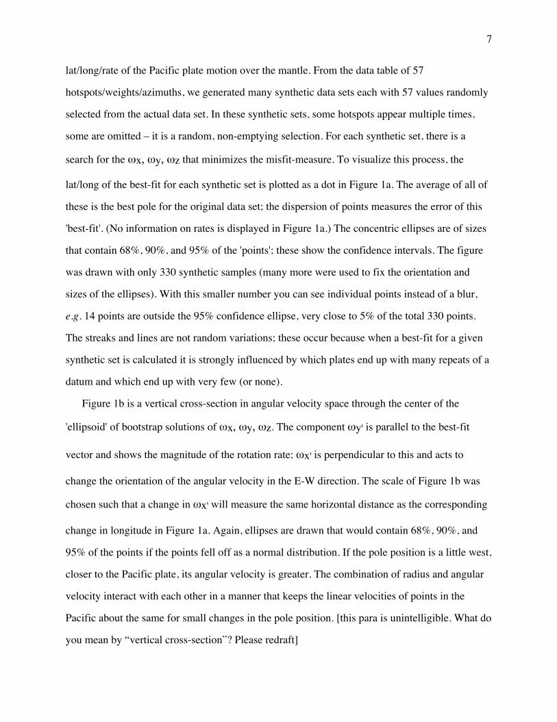
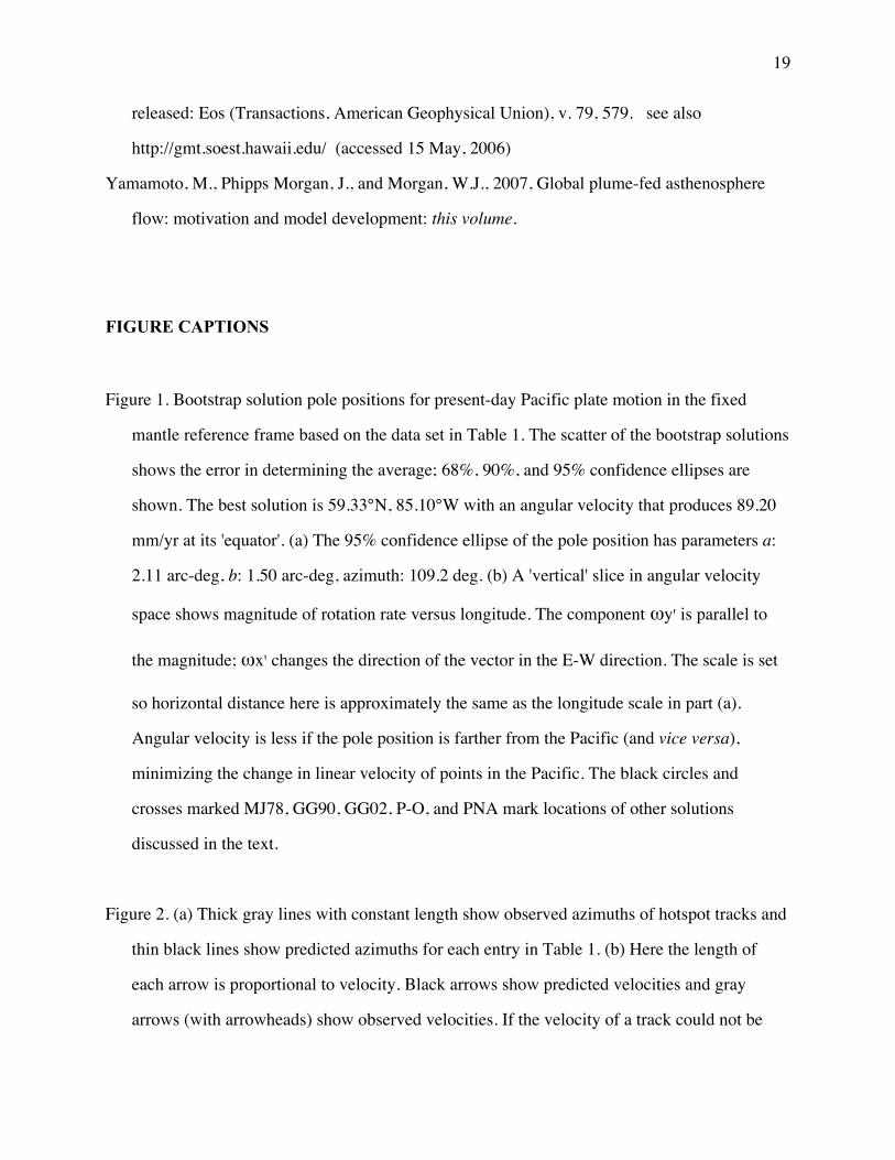
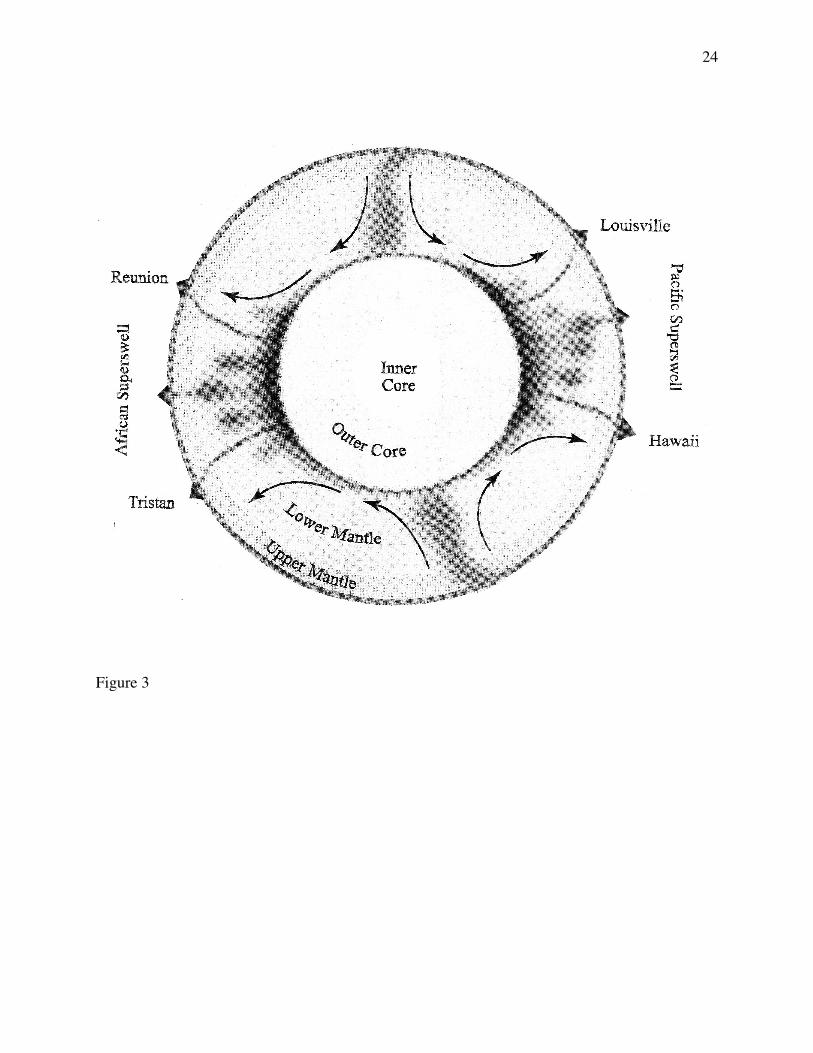
We think the geodynamic nature of this region is perhaps best interpreted as shown in Figure
4 of Courtillot et al. (2003) or Figure 14 of Davaille et al. (2003). An important variation of this
is shown in Figure 2 of Jellinek et al. (2003) or Figure 4 of Gonnermann et al. (2004). In these
figures, we see from shadowgraphs of narrow plumes rising from a hot bottom boundary layer
that the bases and rising columns of plumes get swept toward the regions with the most uprising
– there are thus many, many more plumes in a 'superswell' region. This general pattern is
portrayed even more clearly, but even more schematically, in Figure 17 of Jellinek and Manga
5
(2004; reproduced here as our Figure 3.) Our interpretation of the superswell region is that a very
large amount of upward transport from the core/mantle boundary region overwhelms the normal
geothermal profile of the Earth and leads to consequences not present above narrow rising
plumes. We think for almost all the mantle, asthenosphere (being brought up by plumes from the
core/mantle boundary region) is warmer than the mantle below the asthenosphere; this excess of
(potential) temperature makes the asthenosphere stable against convection from just below. (That
is, a mid-ocean rise has no 2-D style mantle 'roll' rising from deep beneath it, rather the needed
material flows in horizontally from asthenosphere supplied at the nearest plume.) But perhaps an
extreme excess of a broad rising plume in the superswell region creates a mantle with the same
(potential) temperature as asthenosphere, and instabilities that do not exist elsewhere can exist
here. In any case, this is a very anomalous, very interesting region; understanding this will likely
lead to a big advance in geodynamics.
DISCUSSION
What can we conclude from the information presented above and in the electronic
supplement? First, we show two figures from our analysis which uses the observed directions of
hotspot tracks in Table 1 to solve for motions of plates over a fixed mantle reference frame.
From these we show how well a 'fixed reference frame' fits the tracks on all plates. After that, we
will return to the 'superswell' problem.
The plate motion in a fixed reference frame was found in the following manner. The motions
of the major plates are tied together using NUVEL-1A rotations (DeMets et al., 1994). Solving
for the three parameters of one plate, the motions of all plates are determined. We took a starting
trial 3-parameters (ωx, ωy, ωz) for the Pacific, used NUVEL-1A to compute the angular
velocities of other plates and thus predict the azimuths of tracks at each hotspot in our data set,
and then searched for the three parameters that minimized a misfit-measure. Our measure was
6
the sum of the weight of a given track times the absolute value of the difference between the
observed azimuth and the computed azimuth (i.e., minimized ∑ wi x | AZiobs – AZipred | ).
(Almost any minimizing function would give essentially the same result. This scheme downplays
outliers as extreme differences are not squared in the sum.) Azimuth-only data are all that are
needed because the velocities get determined by the NUVEL-1A model – if the choice of pole
position (of the Pacific) is correct but the angular velocity is wrong, tying to other plates would
seriously mismatch the azimuths of motion there. (An azimuths-only scheme was used by Gripp
and Gordon (2002) in one version of their solution, but then they included rate-data for their final
HS3 model.) The advantage of azimuth-only data is azimuths are more accurately observed and
there are no systematic errors as may be present in rate measurements. Many of the tracks are
poorly dated, and K-Ar measurements may have unknown systematic errors. Also, how do you
devise a weighting function to include a track with an accurate azimuth but poorly determined
rate in with the other tracks? We have used azimuths only, and shall test the solution by
comparing it with the measured rates. (A systematic comparison of the measured rates, and their
error estimates, with model-predicted-rates is a major component of our paper-in-progress. Here
we have only a visual comparison as shown in Figure 2b.)
An important concern is azimuths on the Pacific and Nazca plates are determined from
'recent' (0 to ~5 Ma) parts of the tracks whereas on the slower plates the azimuth is generally
defined over a longer period of time (0 to ~10 Ma), and on some of the poorest defined tracks
(Hoggar, Tibesti, Afar, Cape Verde, Kerguelen) over up to ~30 Ma. (The fast-moving Australian
tracks are averaged over a longer period for a different reasons: (1) there are no seamounts in the
Tasmantid chain younger than 5 Ma, and (2) the very straight-line alignment of the inland
volcanics used to find the azimuth of the East Ausralian track range in age from 8 to 17 Ma.)
However, several of the 'slow' tracks are quite narrowly defined in azimuth (Eifel, Canary, St.
Helena, Martin Vaz, Fernando do Noronha, Yellowstone, Raton) and there is no obvious 'kink' in
their tracks to suggest a significant long-term/short-term difference.
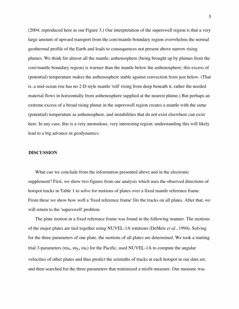
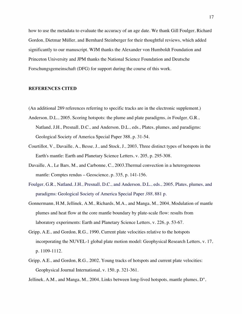
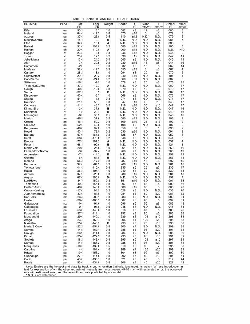
Figure 1 shows how the bootstrap method was used to estimate the uncertainty in the
7
lat/long/rate of the Pacific plate motion over the mantle. From the data table of 57
hotspots/weights/azimuths, we generated many synthetic data sets each with 57 values randomly
selected from the actual data set. In these synthetic sets, some hotspots appear multiple times,
some are omitted – it is a random, non-emptying selection. For each synthetic set, there is a
search for the ωx, ωy, ωz that minimizes the misfit-measure. To visualize this process, the
lat/long of the best-fit for each synthetic set is plotted as a dot in Figure 1a. The average of all of
these is the best pole for the original data set; the dispersion of points measures the error of this
'best-fit'. (No information on rates is displayed in Figure 1a.) The concentric ellipses are of sizes
that contain 68%, 90%, and 95% of the 'points'; these show the confidence intervals. The figure
was drawn with only 330 synthetic samples (many more were used to fix the orientation and
sizes of the ellipses). With this smaller number you can see individual points instead of a blur,
e.g. 14 points are outside the 95% confidence ellipse, very close to 5% of the total 330 points.
The streaks and lines are not random variations; these occur because when a best-fit for a given
synthetic set is calculated it is strongly influenced by which plates end up with many repeats of a
datum and which end up with very few (or none).
Figure 1b is a vertical cross-section in angular velocity space through the center of the
'ellipsoid' of bootstrap solutions of ωx, ωy, ωz. The component ωy' is parallel to the best-fit
vector and shows the magnitude of the rotation rate; ωx' is perpendicular to this and acts to
change the orientation of the angular velocity in the E-W direction. The scale of Figure 1b was
chosen such that a change in ωx' will measure the same horizontal distance as the corresponding
change in longitude in Figure 1a. Again, ellipses are drawn that would contain 68%, 90%, and
95% of the points if the points fell off as a normal distribution. If the pole position is a little west,
closer to the Pacific plate, its angular velocity is greater. The combination of radius and angular
velocity interact with each other in a manner that keeps the linear velocities of points in the
Pacific about the same for small changes in the pole position. [this para is unintelligible. What do
you mean by “vertical cross-section”? Please redraft]
8
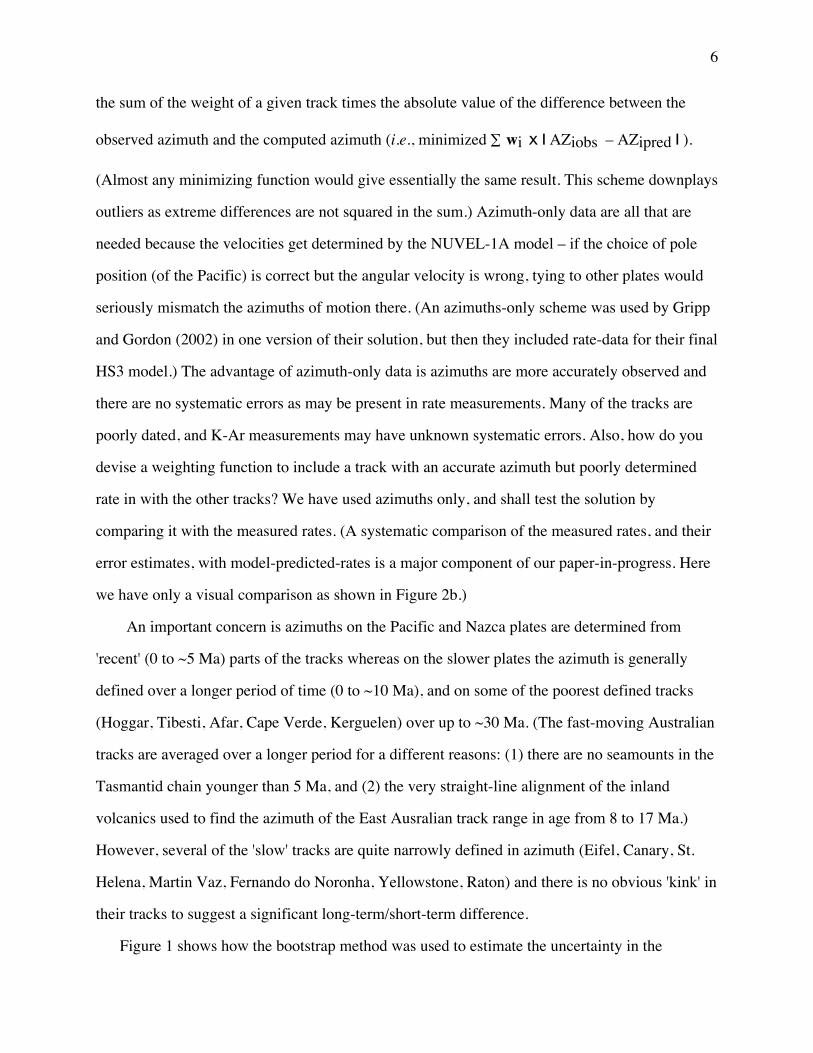
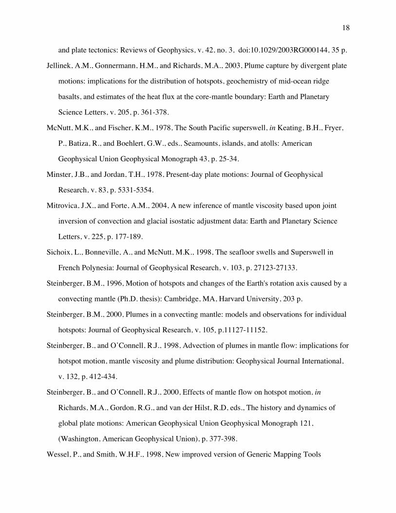
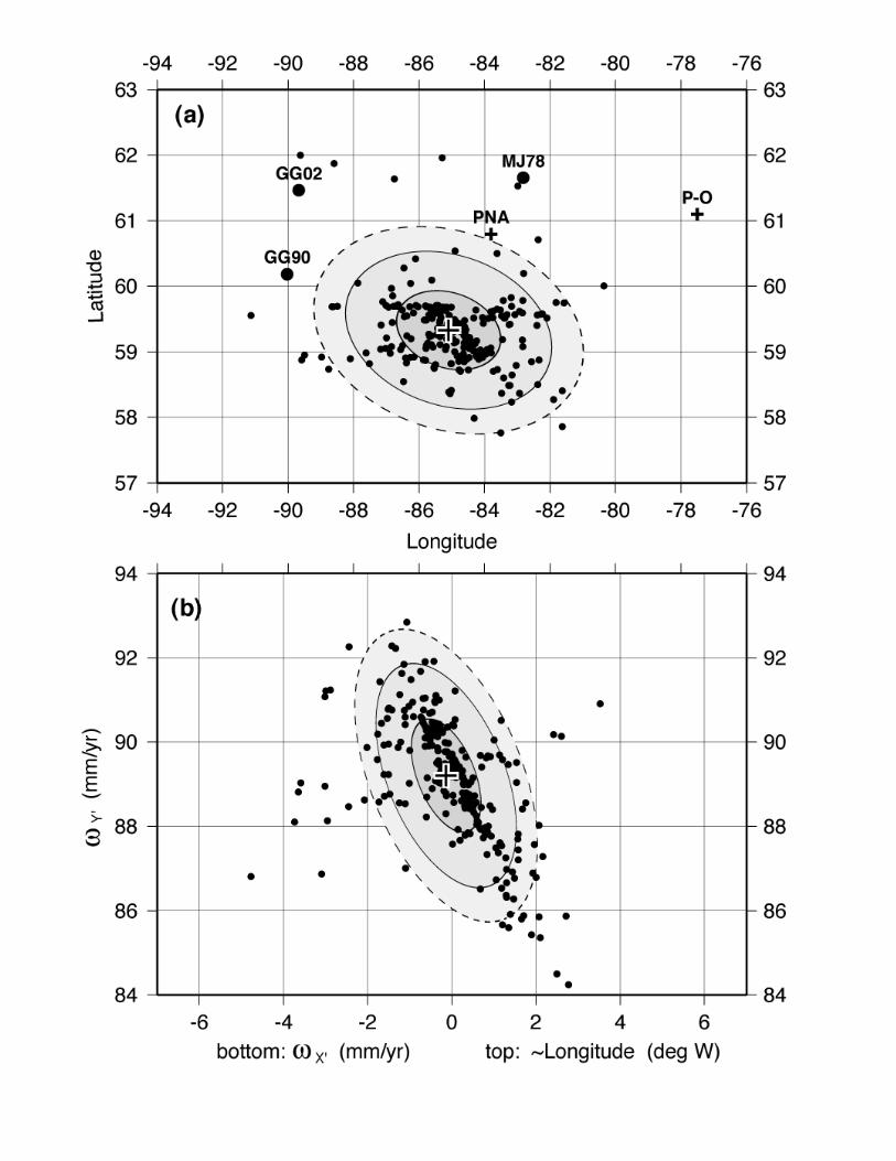
Figure 2 compares our model with the observations listed in Table 1. The top panel shows
the predicted azimuths (black lines) of our model and observed azimuths (gray lines). The
agreement with the azimuth data is quite remarkable. Only three locations have notable
differences between the observed and model directions: Comores, Marquesas, and Louisville.
[This is going to puzzle readers. Many others fit badly, e.g., Balleny, Scott and Canary] We have
no real guess why the Comores track is as it is, for Marquesas we have guessed interaction with a
nearby major fracture zone deflected the track, and for Louisville we have chosen the azimuth of
the recent trend of the Hollister Ridge and not the northern position/track used by others (and
which generates the long-term trend of the entire Louisville chain). The bottom part of the figure
shows arrows whose lengths are proportional to velocity. It shows the model velocities (black
arrows) and the observed velocities (gray arrows). If a velocity has not been observed, a gray line
without an arrowhead is drawn with the direction of the observed azimuth. All high velocities are
in the Pacific or Australian regions, all other plates have very slow velocities over the mantle.
The fit to the velocity data is not as good as above. On a number of tracks (Caroline, Guadalupe,
Macdonald, Arago, Society, Easter, Canary, Reunion, and Crozet) the observed rate is
significantly higher than the model rate. (Note of these, only Canary and Easter have rates based
on 40Ar/39Ar dating, rates for the other seven are based on K-Ar.) We have come to the
conclusion that the azimuth data set is a much cleaner set and the velocity set less reliable.
Velocities are harder to determine – late stage volcanism, delayed volcanism getting through the
lithosphere, and argon-loss in samples due to small degrees of weathering all systematically shift
the age 'too young' (and the rate 'too high'). The most striking feature of Figure 2b is the contrast
between the very high velocities in the Pacific area and very small, even near-zero, velocities on
the other plates. Our model not only duplicates the very slow velocities on these plates but even
correctly predicts the azimuths of tracks on these plates.
Our pole position at 59.33°N, 85.10°W is very similar to that of earlier papers (e.g., Minster
and Jordan, 1978; Gripp and Gordon, 1990; Gripp and Gordon, 2002). Our confidence ellipse is
smaller, but that is a minor difference resulting from the use of a larger data set. What is really
9
different is the rate of angular velocity – ours (89.20 mm/yr or -0.8028 °/yr) is significantly less
than, say, that of Gripp and Gordon (2002). With this slower rotation about essentially the same
pole, the predicted directions of motion of all other plates fits the observed azimuths of their
hotspots tracks. If the angular velocity of the Pacific is 'too high', it adds a westward component
to the motion of all plates which can result in up to ~180° difference between predicted and
observed tracks on very slow moving plates. We tried several variations based on the data in
Table 1. In one case, we used only the 19 very best determined azimuths (those with weight '1'),
in another case we used the 34 'very good' azimuths (those with weights 1 or 0.8), and in a third
case we used all 57 azimuths but gave them all a weight of '1' irrespective of the w listed in the
table. These cases gave solutions 59.38°N, 83.20°W, 87.40 mm/yr; 59.01°N, 83.45°W, 87.96
mm/yr; and 59.66°N, 87.47°W, 89.77 mm/yr respectively. All of these cases fell within the 90%
confidence ellipse shown in Figure 1a. (The error ellipses of these other cases were all larger
than our 'best' solution shown in Figure 1a, generally by a factor between 1.5 and 2.)
Then we chose a data set consisting of the 37 tracks that were 'non-Pacific', i.e., omitting
those tracks on the Pacific, Nazca, or Cocos plates. This data set gave a solution of 59.32°N,
85.00°W, 89.18 mm/yr – almost identical to our solution using all the data. Thus we find no
difference from the pole of non-Pacific hotspots and the pole using all the tracks. Next we chose
a data set where only the 20 tracks on the Pacific, Cocos, or Nazca plates were used. These gave
a solution of 61.1°N, 77.5°W, 83.2 mm/yr but with very large uncertainties: the 95% ellipse had
a semi-major axis of 24 arc-deg, semi-minor 8 arc-deg, with the long-axis along an azimuth of
069°. (This 'Pacific only' pole is marked with a cross labeled 'P-O' in Figure 1a.) This large
uncertainty was expected from the azimuth-only technique; with the data essentially all on the
same plate, the lines perpendicular to the tracks are all near parallel – no cross-cutting constraints
to refine the position in the 'long-direction'. We would need velocity vs. distance data to pin
down the best pole on this long 'smear', just as both fracture zone trends and spreading rates are
needed to accurately fix a pole for the relative motion between two plates. We then chose a
slightly larger data set, the 20 'Pacific' tracks above plus Yellowstone and Raton on the North
10
American plate and the East Australian, Tasmantid, and Lord Howe tracks on the Australian
plate (reasoning these are nearby and might be part of a 'Pacific set'). This gave a solution of
60.8°N, 83.8°W, 89.2 mm/yr with smaller but still large uncertainties, for 95%, a= 12 arc-deg,
b= 7 arc-deg, azimuth= 040°. (This 'Pacific' plus North America plus Australia pole is marked
with a cross labeled 'PNA' in Figure 1a.) However, there was no need to find the pole for 'Pacific
only' motion ourselves. The papers by Minster and Jordan (1978) and Gripp and Gordon (1990;
2002) have already done this. The Minster and Jordan (1978) and Gripp and Gordon (1990)
papers use only data from the Pacific-Cocos-Nazca plates plus only one other bit of data – the
azimuth of the Yellowstone track in North America. The Gripp and Gordon (2002) paper uses
data from the Pacific area and Yellowstone plus only one other bit of data – the azimuth of the
Martin Vaz/Trindade trend on the South American plate. These three poles are shown in Figure
1a, marked MJ78, GG90, and GG02. They are all within ~3 arc-deg of our pole that best-fits the
'non-Pacific' set: the 37 tracks not on the Pacific or Cocos or Nazca plates. (Recall the 'non-
Pacific' pole is practically on top of our pole that best-fits all 57 tracks.)
We conclude, for present-day motion, that a single reference frame fits the entire world – the
hotspots as a group in the 'Pacific' do not drift relative to a group centered on 'Africa'. The
various poles for 'Pacific' are ~3° from our pole for 'non-Pacific', just outside our error ellipse but
our pole is well within the larger error ellipses of these three earlier studies. The rates about these
poles are different; our rate is ~89 mm/yr, theirs average about 20% higher (~110 mm/yr). If the
hotspots on opposite sides were to drift relative each other, we find it very strange they would
both move about the same pole but have different rates about this pole – why not a totally
different pole if one side moves relative to the other? Note also our slower rate is close to the
average rate of Pacific motion for the past 47 Ma – the higher rate of other models needs to have
been much slower earlier or the Pacific tracks would get to the 'Emperor bend' too soon. Our
conclusion is earlier studies have chosen a 'too high' velocity, biased by systematics in the rate
measurements of the hotspot tracks.
Could the rates of track migration on the Pacific plate be high because the mantle and hotspot
11
pipes themselves are being pushed away from the Japan/Marianas centers of subduction? That is,
the high velocity measurements in the Pacific are correct but there is this added component as
explained in several papers by Berhard Steinberger (e.g., Steinberger, 2000; Steinberger and
O'Connell, 1998; 2000). We think this pipe-drift effect is real, but that the rates of hotspot drift
are not ~20 mm/yr as needed to explain the difference between our model and the earlier models.
In a simple mass balance, a 200-km-thick slab descending into the lower mantle at 100 mm/yr
creates a volume flux that can be matched by a 2000-km-thick slab of lower mantle moving
horizontally at 10 mm/yr, or, with half the flow going in each direction, at ~5 mm/yr. This effect
might have strong influence at some sites (say, Caroline), but could not cause all the tracks in the
Pacific to drift west-to-east at the ~20 mm/yr needed to reconcile the earlier models to ours.
Further, the ~5 mm/yr is probably on the high side – even 5 mm/yr drift of hotspots would play
havoc with the strikingly good model-to-data fit of azimuths on the slower plates.
SOME INFERENCES
Given this background, that we find strong support for a model of rigid plates over a fixed
mantle reference frame, we wish to discuss two issues that came up during our compilation of
the data for each track. The first is the closeness of pairs of hotspots, the second is the
'superswell problem'.
There are a number of hotspots that are very near other hotspots – so close it suggests they
cannot be independently anchored deep in the mantle at the core-mantle boundary. In particular,
the pairs Tristan/Gough, Madeira/Canary, Eifel/Massif Central, Kerguelen/Heard, Eastern
Australia/Tasmantid, Easter/Crough, and Cobb/Pratt-Welker (Bowie). A possible explanation for
this without changing the fixity of hotspots is as follows. Suppose in the initial, flood-basalt
stage of a plume, a large 'pipe' 300 km across develops to rapidly carry the large volume to the
surface. The excess temperature of the ascending plume causes 'zone refinement' in the mantle
surrounding the pipe. The higher temperature and increased diffusion rate 'sucks out' volatiles
12
from the surrounding mantle, leaving a wall a few tens of kilometers thick. Without the volatiles,
this wall is 'tougher' than normal mantle. Then, as the large plume flux fades away, the 300 km
diameter tube is too large for the flux it carries. The tube starts to collapse, flattening into an
elongate elliptical cross-section. As the upward flux continued to decrease, opposite sides of the
tube might touch each other sealing off the center. But the two distal portions would remain open
because the 10+ km thick tough rind flexes with a minimum radius, not deforming into a tight
crease that would seal the tips. If something like this were so, what might be tests? Three
observations might be: (1) the pairing would occur long after a flood basalt stage, (2) at the very
end of a plume's life, the flux might become too low to supply two conduits and one might
disappear by starvation, and (3) the plane between the two 'tips' would be oriented perpendicular
to the maximum horizontal compressive stress in the lower mantle.
How can the superswell region, with its (1) shallower-than-normal seafloor, (2) numerous
short volcanic chains that appear to turn on/turn off with time scales of ~10 Ma rather than the
~100 Ma typical of many hotspots, and (3) a warmer-than-typical mantle (see the section
'Superswell Region' located in the main text just after the discussion on the Marquesas Islands
for details), be reconciled with our model of a global, mantle-fixed reference frame? We assume
a very, very weak asthenosphere that almost completely decouples the plates from the mantle
below. (This decoupling is less complete beneath old parts of continents, consequently plates
with large areas of shield/platform move slower over the mantle than do largely 'oceanic' plates.)
In a recent paper on mantle viscosity, Mitrovica and Forte (2004, Fig. 1c,d) find a low-viscosity
channel below the lithosphere, a higher viscosity just beneath the asthenosphere, and then a
much higher viscosity in the lower mantle (until very near the core-mantle boundary). In
averages we made when we re-chose the depth of boundaries between regions, we get from their
Figures 1c and 1d the following: η = 5 x 10¹⁹ Pa-s between 100 km and 300 km, η = 5 x 10²⁰ Pa-s
between 300 km and 660 km, and η ≈ 2 x 10²² Pa-s in the lower mantle. This general pattern,
with a low-viscosity asthenosphere channel and higher-viscosity lower mantle and with
approximately the same ratios between high and low viscosities, was also found by Panasyuk
13
and Hager (2000, Fig. 5a,b). In our analysis of horizontal flow in an asthenospheric channel, we
found an average viscosity of the asthenosphere of 7 x 10¹⁸ Pa-s (Yamamoto et al., 2007, caption
to Fig. 16). (In this analysis, we assumed the base of the asthenosphere was at 300 km – the
thickness of the asthenosphere was ~200 km, varying slightly as the lithosphere thickened with
age. If the asthenosphere viscosity were greater than 7 x 10¹⁸ Pa-s, there would be too much 'pile
up' and corresponding lift of the seafloor because of the pressure gradient created by plate drag
as the Pacific moves westward toward the Mariana and Japan trenches.)
Using these viscosities and thicknesses (~1 x 10¹⁹ Pa-s in a 200 km thick asthenosphere, ~5 x
1020 Pa-s between ~400 km to 660 km, and ~2 x 10²² Pa-s in a ~2000 km thick lower mantle),
we get roughly the following. If a hotspot source is well anchored near 660 km at the base of the
transition zone, its 'drift' relative to the 'fixed' frame would be only ~1/20 of the horizontal
motion of the plate above (assuming uniform shear stress in the layers). If it is anchored at the
base of the mantle, its drift would be even less – determined by horizontal flow in the lower
mantle forced by 'mass balance' of what is being injected in at subduction zones. (However,
much of the horizontal transport in the lower mantle could be very high velocities in the low-
viscosity D" layer and not slow horizontal velocities distributed throughout the lower mantle.)
The fixity of hotspots has been one of the main arguments favoring their sources being near the
core-mantle boundary. We have shown in the bulk of this paper that this fixity is even stronger
than previously thought, but if this fixity is due to a near-inviscid asthenosphere decoupling the
plates from all mantle below, this is no longer a reason to place the sources at the base of the
mantle. However we think there are other arguments favoring the deep origin of plumes.
In our model, all asthenosphere is created by plumes bringing material up from D". This is a
very large flux: the total upward flow in all plume pipes is ~300 km3/yr – the same as the
downward flux of all slabs. The asthenosphere is very hot – it is the temperature of D" minus
only the adiabatic effect as the plume rises to asthenosphere depth. The subducting slabs carry
'coldness' into the mantle. These are gradually warmed up by conduction inward from the
14
surrounding mantle (extracting heat from a larger volume), by internal radioactivity over their
trip-time of order billion years, plus the added input for the short time material is in D" before
coming back to the asthenosphere. This pattern of convection would produce an asthenosphere
hotter than the mantle below it. Downward conduction of heat from the asthenosphere would
make an isothermal temperature gradient in the transition-zone region between the base of the
asthenosphere and the 660-km discontinuity (and somewhat below the 660-km discontinuity, or
at least reduce the temperature increase with depth to below the adiabatic gradient. Thus the
mode of convection we are suggesting would act as an on/off switch – if the plumes bring up
enough hot material from D" depths to make a hot asthenosphere, then this turns off all other
convection from the mid-mantle/660-km discontinuity into the upper mantle. That is, adiabatic
cooling of material starting from mid-mantle or 660-km depths would be cooler than the
shallower levels it would be trying to reach and so such modes of convection (such as rising
from below the EPR to supply the spreading ridge with material) would be turned off. This
model requires 'enough' material be brought up by plumes and that the material spread out easily
from where there are 'sources' of asthenosphere (above plumes) to where there are 'sinks' of
asthenosphere (mid-ocean ridges). We do not know how much is 'enough', but once this limit is
reached, it becomes the only mode of convection.
We think the plate-tectonic cycle adjusts its rate to equal what is brought up by plumes. If
plume rates were to decrease, the asthenosphere would thin, plate drag would increase, and
subduction rates slow down. Contrariwise, if plumes were more vigorous, plate drag would
decrease and movement toward subduction zones would be faster. There may be cycles of
fluctuations tens of millions of years long in this. For example, at the time of a flood basalt the
asthenosphere may temporarily increase in volume, the asthenosphere then thinning as this
excess is used up (the Cretaceous super-cycle may be such a case) – but the long-term rate is set
by the plumes. (Many consequences of this pattern of flow are explored in Yamamoto et al., this
volume.)
This pattern of flow can efficiently extract heat from the Earth's interior and set the rate for
15
plate tectonics, but how can it be applied to the superswell region? Why would a small area of
the Pacific (only 5% of the Earth's surface) have a quarter of the world's hotspot tracks? A
slightly larger region (~10% of the Earth) on the African side has another quarter of all hotspots.
If the long-term convection scheme remains more or less the same for some long period of time,
this could 'sweep' the rising plumes into a central region – the pattern shown schematically in
Figure 3 (adapted from Figure 17 in Jellinek and Manga, 2003), is a highly schematicized
interpretation of the plume/tank experiments shown in Figure 4 of Gonnermann et al., 2004.)
This same idea is nicely illustrated in Figure 11 of Steinberger and O'Connell (1998) and is
clearly stated on page 76 of Steinberger's thesis (Steinberger, 1996): "This raises another
possibility - plumes might be stationary where they are, not because flow in the mantle is so
slow, but because they already have been advected into large-scale stationary upwellings in the
lower mantle, ...".
Convective overturn is what removes interior heat by bringing mantle close to the top surface
where its heat is lost through the surface by conduction. We think the asthenosphere is hotter
than mantle beneath it, cutting off any upwelling from the transition zone into the asthenosphere
except for where there are rising plumes and possibly the superswell region as discussed below.
This does not mean there are no up and down motions in the mantle except sinking slabs and
rising plumes. Rather any secondary interior flow induced by denser slabs and buoyant plumes
will not lead to heatloss through the surface – in this sense slow interior flow is only of
secondary importance to Earth’s convective heat transport.
For most of the Earth, a 'hotspot' at the surface is an indication of a plume rising from deep.
The exception is in the superswell region. If a plume, or group of plumes, remains in one place in
the mantle for 100's of millions of years, the outward conduction of heat from the rising pipe
would spread out into the surrounding mantle. If it conducts outward ~100 km in 100 Ma; it
would conduct outward ~300 km in 1 b.y. If rheology depends on temperature and volatile
content, the high temperature alone would make the mantle surrounding a pipe less viscous than
'average' mantle, but a 'zone-refining' effect as discussed above would increase the viscosity of
16
the region around a pipe. The net result may be the mantle around a pipe is 'hotter' but not
significantly less viscous than other parts. Thus in the superswell region, the usual 'stable'
geotherm pattern (where asthenosphere is hotter than mantle below) is overwhelmed. Here
relatively shallow convective instabilities could occur as temperatures at the 660-km-
discontinuity and mantle above this might be hotter than asthenosphere (because of the long-term
outward conduction of heat into the mantle from the stable pipes). Short-term instabilities could
then rise into the asthenosphere, creating short-lived tracks. In our model of viscosity structure of
the upper mantle (from Mitrovica and Forte, 2004; Panasyuk and Hager, 2000; Yamamoto et al.,
2007) the mantle between ~400-660 km is considerably more viscous than asthenosphere and
would have small velocities compared to fast plate motion. Thus observed tracks at the surface
would be all near-parallel to plate motion and all have migration rates very close to the velocity
of the plate – rooted in the lower transition zone would be nearly as 'fixed' as rooted at the core-
mantle-boundary, just not have the long lifetime. A scheme like this (the main features of which
could be validated with numerical modeling) reconciles the model of plumes rising from the
core-mantle boundary as the primary pattern of mantle convection with the conundrum of so
many hotspots, many short-lived, and many close together, as was forcefully argued in the book
'Plates, Plumes, and Paradigms' (Foulger et al., 2005).
ACKNOWLEDGEMENTS
[Appropriate in electronic supplement] WJM thanks the Department of Earth and Planetary
Sciences at Harvard for welcoming him as a visiting researcher. For the tracks on land, the map
collection at the Princeton University library was invaluable – for tracks in the oceans, the
synthetic-bathymetry of W. H. F. Smith and D. T. Sandwell (version 7.2) was our primary
source. Blowup plots of the bathymetry defining the ocean tracks were easy to make because of
the GMT software of P. Wessel and W. H. F. Smith (1998), and we especially thank W.H.F.S.
for showing us a work-around to a plotting difficulty we encountered. Ajoy Baksi showed us
17
how to use the metadata to evaluate the accuracy of an age date. We thank Gill Foulger, Richard
Gordon, Dietmar Müller, and Bernhard Steinberger for their thoughtful reviews, which added
significantly to our manuscript. WJM thanks the Alexander von Humboldt Foundation and
Princeton University and JPM thanks the National Science Foundation and Deutsche
Forschungsgemeinschaft (DFG) for support during the course of this work.
REFERENCES CITED
(An additional 289 references referring to specific tracks are in the electronic supplement.)
Anderson, D.L., 2005, Scoring hotspots: the plume and plate paradigms, in Foulger, G.R.,
Natland, J.H., Presnall, D.C., and Anderson, D.L., eds., Plates, plumes, and paradigms:
Geological Society of America Special Paper 388, p. 31-54.
Courtillot, V., Davaille, A., Besse, J., and Stock, J., 2003, Three distinct types of hotspots in the
Earth's mantle: Earth and Planetary Science Letters, v. 205, p. 295-308.
Davaille, A., Le Bars, M., and Carbonne, C., 2003,Thermal convection in a heterogeneous
mantle: Comptes rendus – Geoscience, p. 335, p. 141-156.
Foulger, G.R., Natland, J.H., Presnall, D.C., and Anderson, D.L., eds., 2005, Plates, plumes, and
paradigms: Geological Society of America Special Paper 388, 881 p.
Gonnermann, H.M, Jellinek, A.M., Richards, M.A., and Manga, M., 2004, Modulation of mantle
plumes and heat flow at the core mantle boundary by plate-scale flow: results from
laboratory experiments: Earth and Planetary Science Letters, v. 226, p. 53-67.
Gripp, A.E., and Gordon, R.G., 1990, Current plate velocities relative to the hotspots
incorporating the NUVEL-1 global plate motion model: Geophysical Research Letters, v. 17,
p. 1109-1112.
Gripp, A.E., and Gordon, R.G., 2002, Young tracks of hotspots and current plate velocities:
Geophysical Journal International, v. 150, p. 321-361.
Jellinek, A.M., and Manga, M., 2004, Links between long-lived hotspots, mantle plumes, D",
18
and plate tectonics: Reviews of Geophysics, v. 42, no. 3, doi:10.1029/2003RG000144, 35 p.
Jellinek, A.M., Gonnermann, H.M., and Richards, M.A., 2003, Plume capture by divergent plate
motions: implications for the distribution of hotspots, geochemistry of mid-ocean ridge
basalts, and estimates of the heat flux at the core-mantle boundary: Earth and Planetary
Science Letters, v. 205, p. 361-378.
McNutt, M.K., and Fischer, K.M., 1978, The South Pacific superswell, in Keating, B.H., Fryer,
P., Batiza, R., and Boehlert, G.W., eds., Seamounts, islands, and atolls: American
Geophysical Union Geophysical Monograph 43, p. 25-34.
Minster, J.B., and Jordan, T.H., 1978, Present-day plate motions: Journal of Geophysical
Research, v. 83, p. 5331-5354.
Mitrovica, J.X., and Forte, A.M., 2004, A new inference of mantle viscosity based upon joint
inversion of convection and glacial isostatic adjustment data: Earth and Planetary Science
Letters, v. 225, p. 177-189.
Sichoix, L., Bonneville, A., and McNutt, M.K., 1998, The seafloor swells and Superswell in
French Polynesia: Journal of Geophysical Research, v. 103, p. 27123-27133.
Steinberger, B.M., 1996, Motion of hotspots and changes of the Earth's rotation axis caused by a
convecting mantle (Ph.D. thesis): Cambridge, MA, Harvard University, 203 p.
Steinberger, B.M., 2000, Plumes in a convecting mantle: models and observations for individual
hotspots: Journal of Geophysical Research, v. 105, p.11127-11152.
Steinberger, B., and O’Connell, R.J., 1998, Advection of plumes in mantle flow: implications for
hotspot motion, mantle viscosity and plume distribution: Geophysical Journal International,
v. 132, p. 412-434.
Steinberger, B., and O’Connell, R.J., 2000, Effects of mantle flow on hotspot motion, in
Richards, M.A., Gordon, R.G., and van der Hilst, R.D, eds., The history and dynamics of
global plate motions: American Geophysical Union Geophysical Monograph 121,
(Washington, American Geophysical Union), p. 377-398.
Wessel, P., and Smith, W.H.F., 1998, New improved version of Generic Mapping Tools
19
released: Eos (Transactions, American Geophysical Union), v. 79, 579. see also
http://gmt.soest.hawaii.edu/ (accessed 15 May, 2006)
Yamamoto, M., Phipps Morgan, J., and Morgan, W.J., 2007, Global plume-fed asthenosphere
flow: motivation and model development: this volume.
FIGURE CAPTIONS
Figure 1. Bootstrap solution pole positions for present-day Pacific plate motion in the fixed
mantle reference frame based on the data set in Table 1. The scatter of the bootstrap solutions
shows the error in determining the average; 68%, 90%, and 95% confidence ellipses are
shown. The best solution is 59.33°N, 85.10°W with an angular velocity that produces 89.20
mm/yr at its 'equator'. (a) The 95% confidence ellipse of the pole position has parameters a:
2.11 arc-deg, b: 1.50 arc-deg, azimuth: 109.2 deg. (b) A 'vertical' slice in angular velocity
space shows magnitude of rotation rate versus longitude. The component ωy' is parallel to
the magnitude; ωx' changes the direction of the vector in the E-W direction. The scale is set
so horizontal distance here is approximately the same as the longitude scale in part (a).
Angular velocity is less if the pole position is farther from the Pacific (and vice versa),
minimizing the change in linear velocity of points in the Pacific. The black circles and
crosses marked MJ78, GG90, GG02, P-O, and PNA mark locations of other solutions
discussed in the text.
Figure 2. (a) Thick gray lines with constant length show observed azimuths of hotspot tracks and
thin black lines show predicted azimuths for each entry in Table 1. (b) Here the length of
each arrow is proportional to velocity. Black arrows show predicted velocities and gray
arrows (with arrowheads) show observed velocities. If the velocity of a track could not be
20
determined, a gray line with no arrowhead is drawn in the direction of the observed azimuth
(with a length the same as the model velocity).
Figure 3. Schematic diagram (from Jellinek and Manga, 2004) illustrating how long-term
subduction in fixed places (here the Andes and Western Pacific) could push/concentrate the
plumes into the superswell regions.
TABLE 1. AZIMUTH AND RATE OF EACH TRACK
HOTSPOT PLATE Lat(°N)
Long(°E)
Weight Azobs(*)
±(°)
Vobs(mm/yr)
±mm/yr
Azmdl(°)
Vmdl(mm/yr)
Eifel eu 50.2 6.7 1.0 082 ±8 12 ±2 080 5Iceland eu 64.4 -17.3 0.8 075 ±10 5 ±3 072 3Azores eu 37.9 -26.0 0.5 110 ±12 N.D.* N.D. 079 6MassifCentral eu 45.1 2.7 B N.D. N.D. N.D. N.D. 081 5Etna eu 37.8 15.0 A N.D. N.D. N.D. N.D. 083 6Baikal eu 51.0 101.0 0.2 080 ±15 N.D. N.D. 100 5Hainan ch 20.0 110.0 A 000 ±15 N.D. N.D. N.D. N.D.Hoggar af 23.3 5.6 0.3 046 ±12 N.D. N.D. 045 9Tibesti af 20.8 17.5 0.2 030 ±15 N.D. N.D. 042 11JebelMarra af 13.0 24.2 0.5 045 ±8 N.D. N.D. 045 13Afar af 7.0 39.5 0.2 030 ±15 16 ±8 044 16Cameroon af -2.0 5.1 0.3 032 ±3 15 ±5 062 14Madeira af 32.6 -17.3 0.3 055 ±15 8 ±3 061 4Canary af 28.2 -18.0 1.0 094 ±8 20 ±4 070 5GreatMeteor af 29.4 -29.2 0.8 040 ±10 N.D. N.D. 101 4CapeVerde af 16.0 -24.0 0.2 060 ±30 N.D. N.D. 087 8StHelena af -16.5 -9.5 1.0 078 ±5 20 ±3 075 15TristanDaCunha af -37.2 -12.3 A N.D. N.D. N.D. N.D. 080 17Gough af -40.3 -10.0 0.8 079 ±5 18 ±3 079 17Vema af -32.1 6.3 B N.D. N.D. N.D. N.D. 067 17Discovery af -43.0 -2.7 1.0 068 ±3 N.D. N.D. 073 17Shona af -51.4 1.0 0.3 074 ±6 N.D. N.D. 071 17Reunion af -21.2 55.7 0.8 047 ±10 40 ±10 043 17Comores af -11.5 43.3 0.5 118 ±10 35 ±10 047 17Kilimanjiro af -3.0 37.5 B N.D. N.D. N.D. N.D. 047 16Karisimbi af -1.5 29.4 B N.D. N.D. N.D. N.D. 049 16MtRungwe af -8.3 33.9 B+ N.D. N.D. N.D. N.D. 049 16Marion an -46.9 37.6 0.5 080 ±12 N.D. N.D. 106 9Crozet an -46.1 50.2 0.8 109 ±10 25 ±13 102 9Ob-Lena an -52.2 40.0 1.0 108 ±6 N.D. N.D. 107 9Kerguelen an -49.6 69.0 0.2 050 ±30 3 ±1 096 9Heard an -53.1 73.5 0.2 030 ±20 N.D. N.D. 094 9Balleny an -67.6 164.8 0.2 325 ±7 N.D. N.D. 052 6Scott an -68.8 -178.8 0.2 346 ±5 N.D. N.D. 044 5Erebus an -77.5 167.2 A N.D. N.D. N.D. N.D. 037 4Peter_I an -68.8 -90.6 B N.D. N.D. N.D. N.D. 124 1MartinVaz sa -20.5 -28.8 1.0 264 ±5 N.D. N.D. 259 19FernandoDoNoron sa -3.8 -32.4 1.0 266 ±7 N.D. N.D. 260 19Ascension sa -7.9 -14.3 B N.D. N.D. N.D. N.D. 257 19Guyana sa 5.0 -61.0 B N.D. N.D. N.D. N.D. 266 18Iceland na 64.4 -17.3 0.8 287 ±10 15 ±5 292 16Bermuda na 32.6 -64.3 0.3 260 ±15 N.D. N.D. 261 18Yellowstone na 44.5 -110.4 0.8 235 ±5 26 ±5 235 17Raton na 36.8 -104.1 1.0 240 ±4 30 ±20 239 18Azores na 37.9 -26.0 0.3 280 ±15 N.D. N.D. 284 18Anyuy na 67.0 166.0 B- N.D. N.D. N.D. N.D. 157 7LordHowe au -34.7 159.8 0.8 351 ±10 N.D. N.D. 001 63Tasmantid au -40.4 155.5 0.8 007 ±5 63 ±5 000 66EasternAustr au -40.8 146.0 0.3 000 ±15 65 ±3 006 70Cocos-Keeling au -17.0 94.5 0.2 028 ±6 N.D. N.D. 033 70JuanFernandez nz -33.9 -81.8 1.0 084 ±3 80 ±20 081 62SanFelix nz -26.4 -80.1 0.3 083 ±8 N.D. N.D. 080 61Easter nz -26.4 -106.5 1.0 087 ±3 95 ±5 097 61Galapagos nz -0.4 -91.6 1.0 096 ±5 55 ±8 086 48Galapagos co -0.4 -91.6 0.5 045 ±6 N.D. N.D. 045 81Louisville pa -53.6 -140.6 1.0 316 ±5 67 ±5 300 76Foundation pa -37.7 -111.1 1.0 292 ±3 80 ±6 283 88Macdonald pa -29.0 -140.3 1.0 289 ±6 105 ±10 295 88Arago pa -23.4 -150.7 1.0 296 ±4 120 ±20 298 88N.Austral pa -25.6 -143.3 B 293 ±3 75 ±15 296 88Maria/S.Cook pa -22.2 -154.0 0.8 300 ±4 N.D. N.D. 299 88Samoa pa -14.5 -169.1 0.8 285 ±5 95 ±20 301 88Crough pa -26.9 -114.6 0.8 284 ±2 N.D. N.D. 285 89Pitcairn pa -25.4 -129.3 1.0 293 ±3 90 ±15 291 89Society pa -18.2 -148.4 0.8 295 ±5 109 ±10 297 89Samoa pa -14.5 -168.2 0.8 285 ±5 95 ±20 301 88Marquesas pa -10.5 -139.0 0.5 319 ±8 93 ±7 295 88Caroline pa 4.8 164.4 1.0 289 ±4 135 ±20 299 89Hawaii pa 19.0 -155.2 1.0 304 ±3 92 ±3 302 80Guadalupe pa 27.7 -114.5 0.8 292 ±5 80 ±10 294 54Cobb pa 46.0 -130.1 1.0 321 ±5 43 ±3 317 44Bowie pa 53.0 -134.8 0.8 306 ±4 40 ±20 327 42
Note: Entries are the hotspot and plate its track is on, its location (latitude, longitude), its weight ‘w’ (see Introduction intext for explanation of w), the observed azimuth (usually from most recent ~5-10 m.y.) with estimated error, the observedrate with estimated error, and the azimuth and rate predicted by our model. * N.D. = not determined