40
Platform Competition Bryan Hong Dylan Minor
| Date post: | 22-Dec-2015 |
| Category: |
Documents |
| View: | 218 times |
| Download: | 0 times |
Platform Competition
Bryan Hong
Dylan Minor
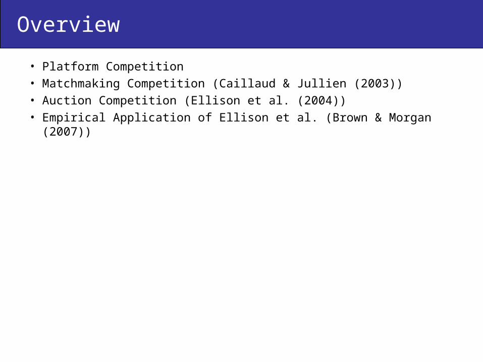
Overview
• Platform Competition• Matchmaking Competition (Caillaud & Jullien (2003))• Auction Competition (Ellison et al. (2004))• Empirical Application of Ellison et al. (Brown & Morgan (2007))

The Game
I E
i
j
?
?
0%
%%

The Tools for Rent Extraction
• Registration Charge• Transaction Charge
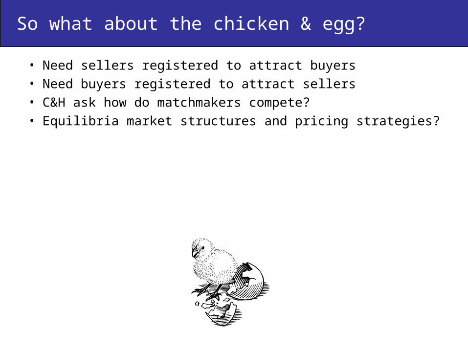
So what about the chicken & egg?
• Need sellers registered to attract buyers
• Need buyers registered to attract sellers
• C&H ask how do matchmakers compete?
• Equilibria market structures and pricing strategies?
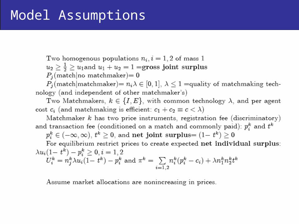
Model Assumptions
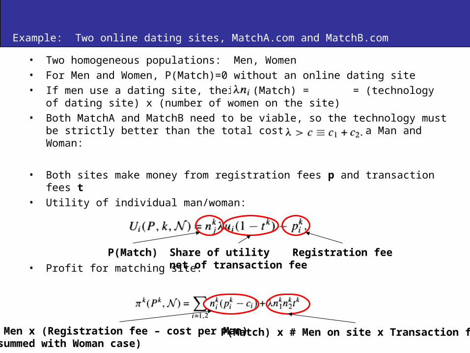
Example: Two online dating sites, MatchA.com and MatchB.com
• Two homogeneous populations: Men, Women• For Men and Women, P(Match)=0 without an online dating site• If men use a dating site, their P(Match) = = (technology of dating site) x (number of
women on the site)• Both MatchA and MatchB need to be viable, so the technology must be strictly better
than the total cost of matching a Man and Woman:
• Both sites make money from registration fees p and transaction fees t• Utility of individual man/woman:
• Profit for matching site:
P(Match) Share of utilitynet of transaction fee
Registration fee
# Men x (Registration fee – cost per Man)(summed with Woman case)
P(Match) x # Men on site x Transaction fee
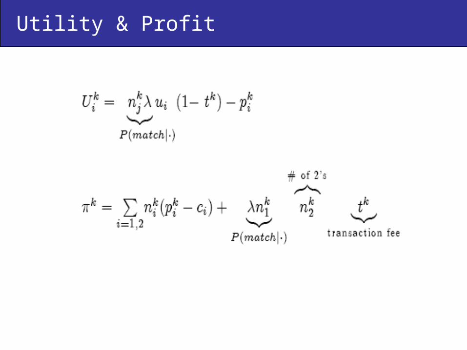
Utility & Profit
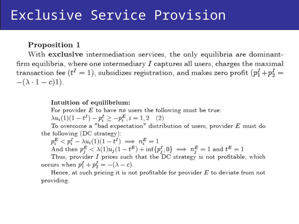
Exclusive Service Provision
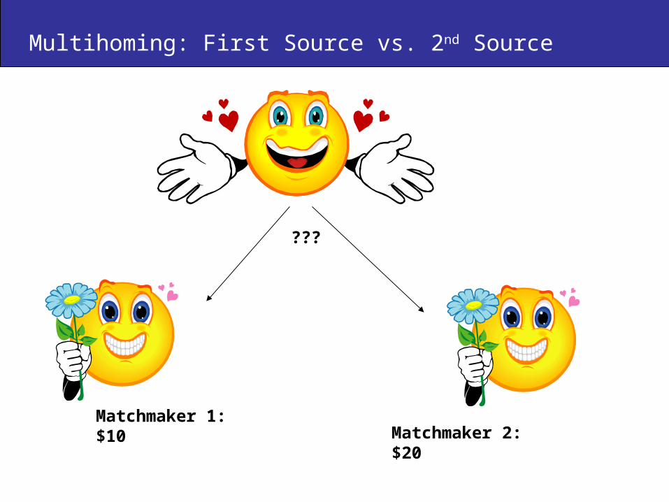
Multihoming: First Source vs. 2nd Source
Matchmaker 1: $10Matchmaker 2: $20
???
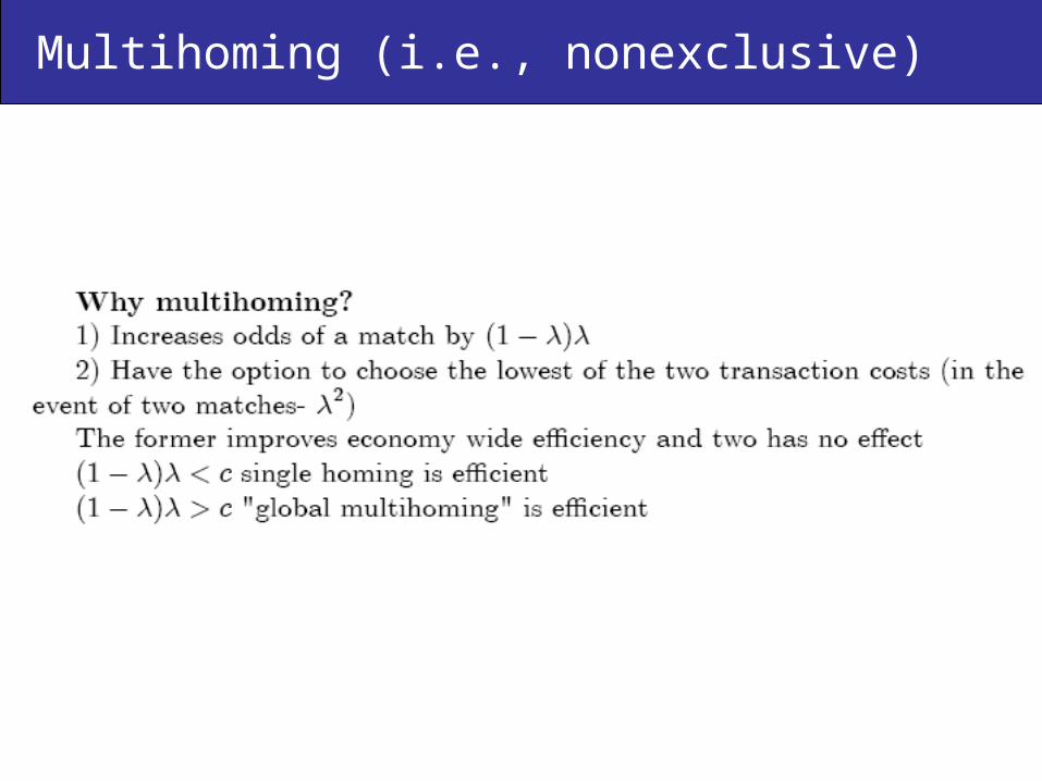
Multihoming (i.e., nonexclusive)
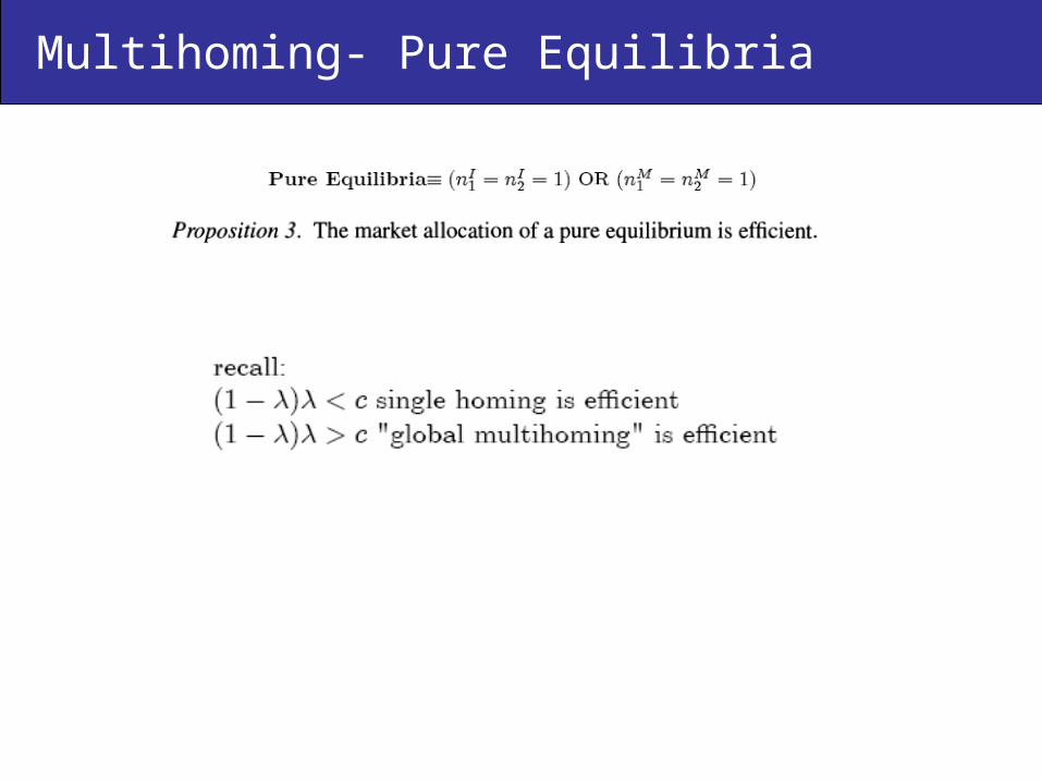
Multihoming- Pure Equilibria

Multihoming- Pure Equilibria
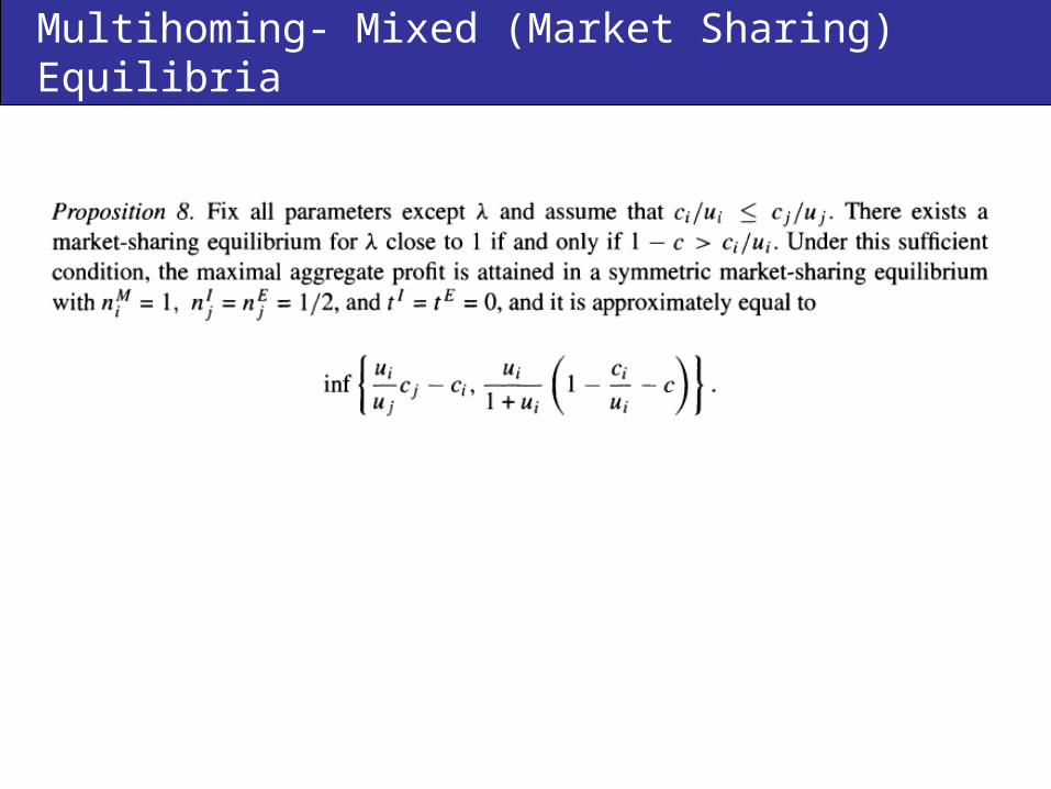
Multihoming- Mixed (Market Sharing) Equilibria
Summary
• Consumer Welfare: highest under exclusivity • Intermediation Profits: with exclusivity the firm makes vanishing
profits; without exclusivity firms earn strictly positive profit• Endogenous Exclusivity: first mover chooses exclusive service if
technology is really great, otherwise generally invites entry• Transaction Fees: exclusivity means transaction fees used for
additional rent extraction; non-exclusivity means can still be used, but can be lower or higher to be first or second source (or zero if dominant-firm or market sharing)
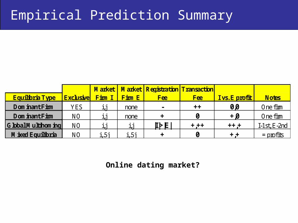
Empirical Prediction Summary
Market Market Registration TransactionEquilibria Type Exclusive Firm I Firm E Fee Fee I vs. E profit Notes
Dominant Firm YES i,j none - ++ 0,0 One firm
Dominant Firm NO i,j none + 0 +,0 One firm
Global Multihoming NO i,j i,j |I|>|E| +,++ ++,+ I-1st, E-2nd
Mixed Equilibria NO i,.5j i,.5j + 0 +,+ = profits
Online dating market?
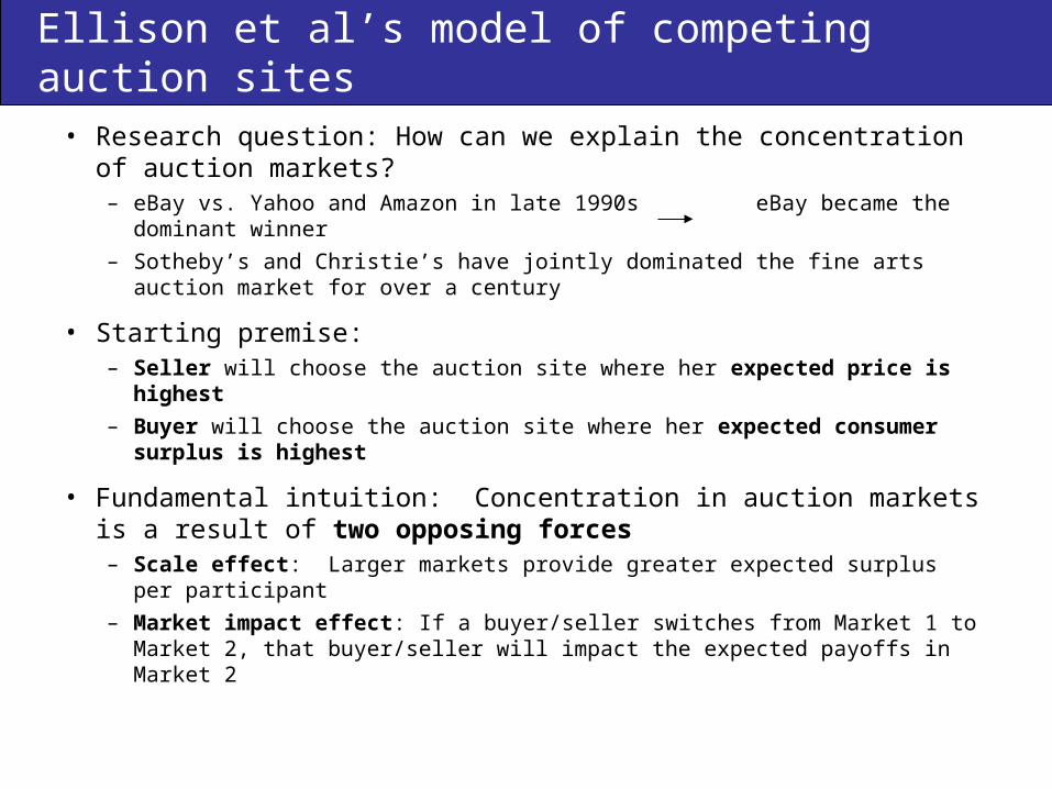
Ellison et al’s model of competing auction sites
• Research question: How can we explain the concentration of auction markets?– eBay vs. Yahoo and Amazon in late 1990s eBay became the dominant
winner
– Sotheby’s and Christie’s have jointly dominated the fine arts auction market for over a century
• Starting premise:– Seller will choose the auction site where her expected price is highest
– Buyer will choose the auction site where her expected consumer surplus is highest
• Fundamental intuition: Concentration in auction markets is a result of two opposing forces– Scale effect: Larger markets provide greater expected surplus per
participant
– Market impact effect: If a buyer/seller switches from Market 1 to Market 2, that buyer/seller will impact the expected payoffs in Market 2
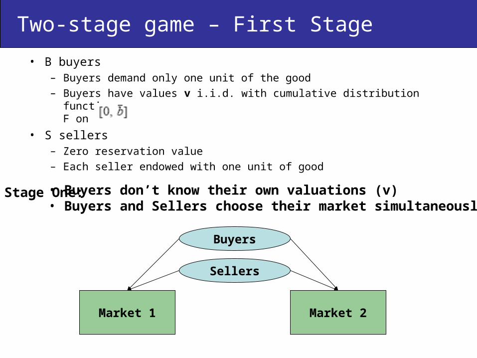
Two-stage game – First Stage
Market 1 Market 2
Stage One:
Buyers
Sellers
• Buyers don’t know their own valuations (v)• Buyers and Sellers choose their market simultaneously
• B buyers– Buyers demand only one unit of the good
– Buyers have values v i.i.d. with cumulative distribution functionF on
• S sellers– Zero reservation value
– Each seller endowed with one unit of good
Sellers Buyer Valuations(decreasing)
Seller 1 Buyer 1
Seller 2 Buyer 2
Seller 3 Buyer 3
Buyer 4
Buyer 5
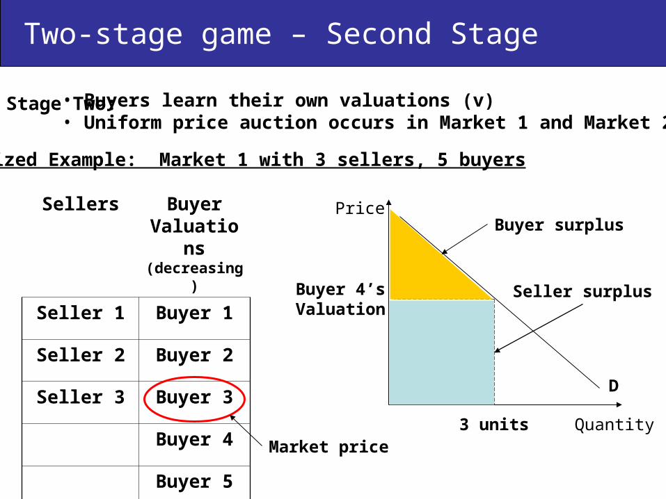
Two-stage game – Second Stage
Stage Two: • Buyers learn their own valuations (v)• Uniform price auction occurs in Market 1 and Market 2
Stylized Example: Market 1 with 3 sellers, 5 buyers
Market price
Buyer 4’sValuation
Price
Quantity3 units
Buyer surplus
Seller surplus
D
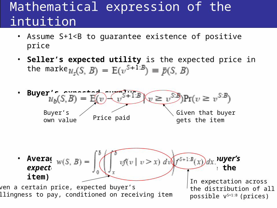
• Assume S+1<B to guarantee existence of positive price
• Seller’s expected utility is the expected price in the market she chooses
• Buyer’s expected surplus
• Average total surplus per unit sold (or, buyer’s expected willingness to pay, given they receive the item)
Mathematical expression of the intuition
Buyer’s own value Price paid
Given that buyer gets the item
Given a certain price, expected buyer’s willingness to pay, conditioned on receiving item
In expectation acrossthe distribution of all possible vS+1:B (prices)

Equilibrium constraint conditions• Two market setup
– Market 1 has B1 number of buyers, S1 number of sellers– Market 2 has B2 buyers, S2 sellers
• Equilibrium exists if and only if the following are true
• Relax condition (I) to allow S1, S2, B1, B2 to be non-integers– Allows for quasi-equilibria
• Identical to “true” equilibria except it ignores the integer constraint
– Purpose of quasi-equilibria is to simplify the analysis– In large markets, ignoring integer constraints doesn’t meaningfully change the results
Utility from staying in Market 1
Utility from switching to Market 2
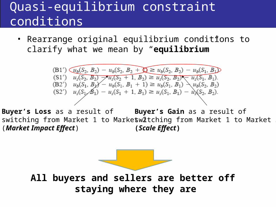
Quasi-equilibrium constraint conditions
• Rearrange original equilibrium conditions to clarify what we mean by “equilibrium”
Buyer’s Loss as a result of switching from Market 1 to Market 2(Market Impact Effect)
Buyer’s Gain as a result of switching from Market 1 to Market 2(Scale Effect)
All buyers and sellers are better off staying where they are
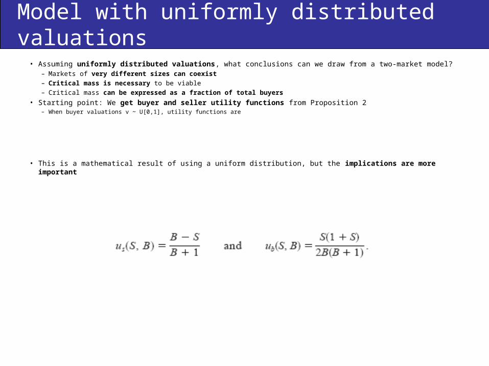
Model with uniformly distributed valuations
• Assuming uniformly distributed valuations, what conclusions can we draw from a two-market model?– Markets of very different sizes can coexist– Critical mass is necessary to be viable– Critical mass can be expressed as a fraction of total buyers
• Starting point: We get buyer and seller utility functions from Proposition 2– When buyer valuations v ~ U[0,1], utility functions are
• This is a mathematical result of using a uniform distribution, but the implications are more important

Implications of larger scale markets
• Per capita surplus scale advantage of the larger market:– Assume Market 2 is the larger market
• Larger market yields higher surplus per capita
• Gain/loss of switching to a larger market for buyers and sellers:
• Buyers are better off in the smaller market because expected price is lower (and vice versa for sellers)
Gamma is used here to denote a constant ratio of sellers to buyers
Main idea is that this isgreater than zero
> 0
> 0
< 0
Seller
Buyer
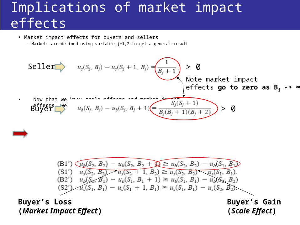
Implications of market impact effects
• Market impact effects for buyers and sellers – Markets are defined using variable j=1,2 to get a general result
• Now that we know scale effects and market impact effects, we can now solve for our quasi-equilibria
Seller
Buyer
Buyer’s Loss(Market Impact Effect)
Buyer’s Gain(Scale Effect)
> 0
> 0
Note market impact effects go to zero as Bj -> ∞
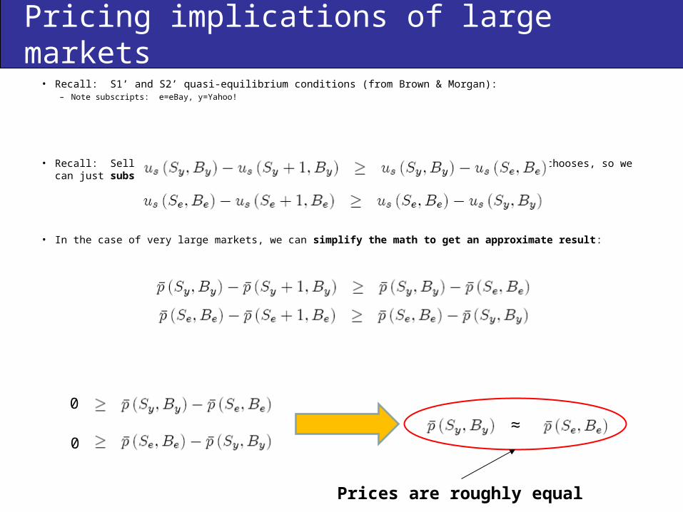
Pricing implications of large markets
• Recall: S1’ and S2’ quasi-equilibrium conditions (from Brown & Morgan):– Note subscripts: e=eBay, y=Yahoo!
• Recall: Seller’s expected utility is just the expected price in the market she chooses, so we can just substitute:
• In the case of very large markets, we can simplify the math to get an approximate result:
0
0≈
Prices are roughly equal
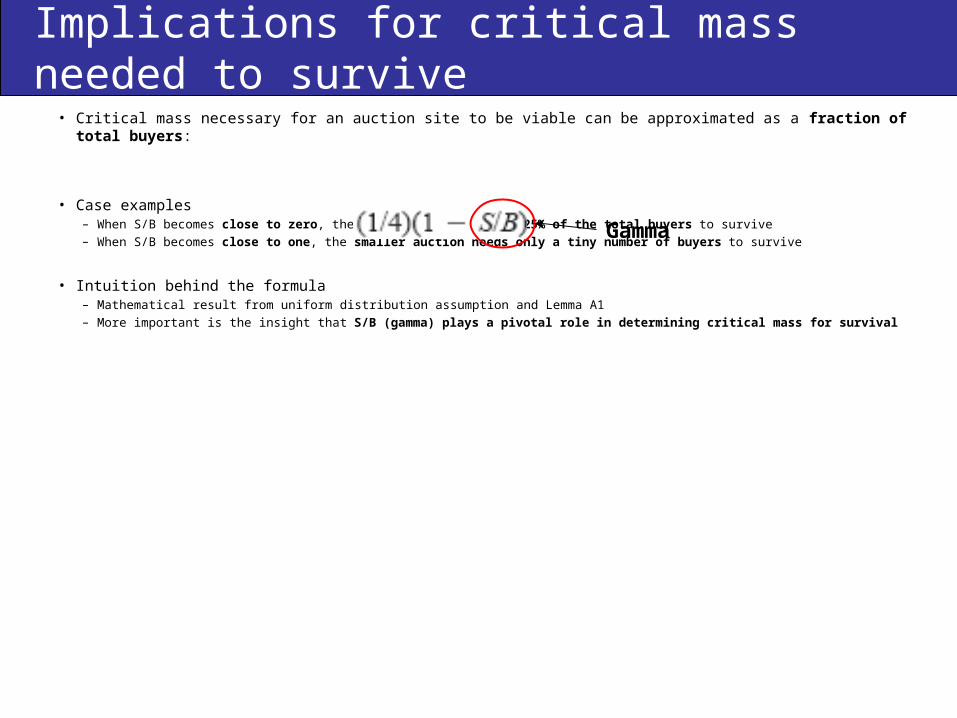
Implications for critical mass needed to survive
• Critical mass necessary for an auction site to be viable can be approximated as a fraction of total buyers:
• Case examples– When S/B becomes close to zero, the smaller auction needs 25% of the total buyers to survive– When S/B becomes close to one, the smaller auction needs only a tiny number of buyers to survive
• Intuition behind the formula– Mathematical result from uniform distribution assumption and Lemma A1– More important is the insight that S/B (gamma) plays a pivotal role in determining critical mass for survival
Gamma
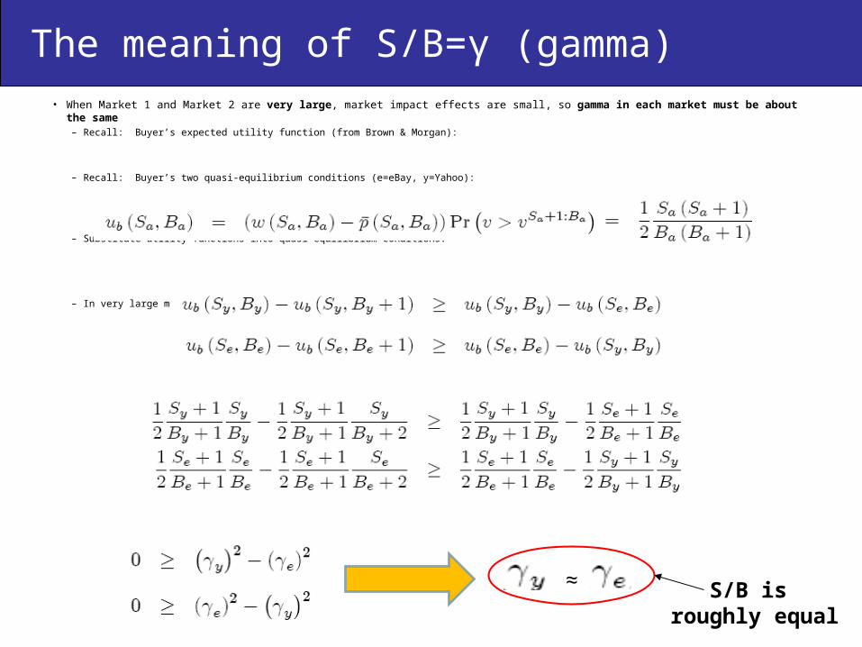
• When Market 1 and Market 2 are very large, market impact effects are small, so gamma in each market must be about the same– Recall: Buyer’s expected utility function (from Brown & Morgan):
– Recall: Buyer’s two quasi-equilibrium conditions (e=eBay, y=Yahoo):
– Substitute utility functions into quasi-equilibrium conditions:
– In very large markets we can reduce the inequalities to:
The meaning of S/B=γ (gamma)
≈ S/B is roughly equal
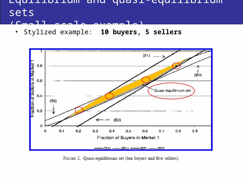
Equilibrium and quasi-equilibrium sets (Small scale example)
• Stylized example: 10 buyers, 5 sellers
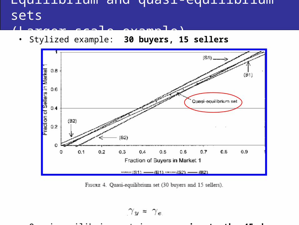
Equilibrium and quasi-equilibrium sets (Larger scale example)
• Stylized example: 30 buyers, 15 sellers
• Quasi-equilibrium set is converging to the 45 degree line because as markets get very large,
≈
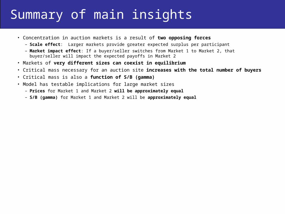
Summary of main insights
• Concentration in auction markets is a result of two opposing forces– Scale effect: Larger markets provide greater expected surplus per participant
– Market impact effect: If a buyer/seller switches from Market 1 to Market 2, that buyer/seller will impact the expected payoffs in Market 2
• Markets of very different sizes can coexist in equilibrium
• Critical mass necessary for an auction site increases with the total number of buyers
• Critical mass is also a function of S/B (gamma)
• Model has testable implications for large market sizes– Prices for Market 1 and Market 2 will be approximately equal
– S/B (gamma) for Market 1 and Market 2 will be approximately equal

Brown & Morgan (2007)
• Field Experiment Results: both rejected with price being 20-70% greater on Ebay and an average of 2 more buyers per seller vs. equivalent Yahoo auction
• Market tipping or equilibrium?...or wrong model?

The End
Appendix for C&H

Multihoming
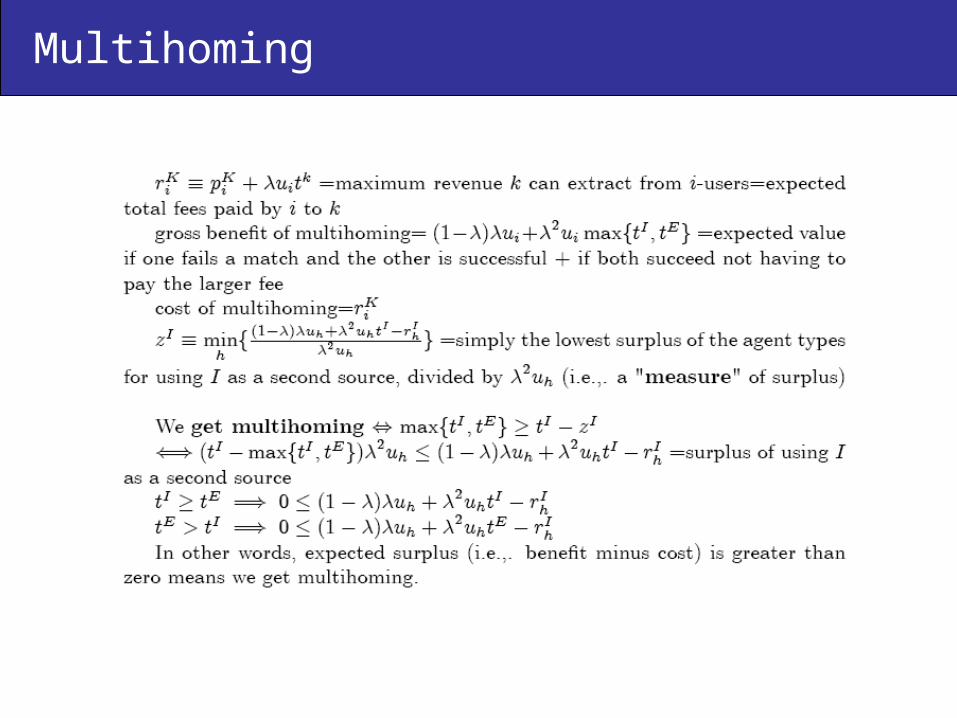
Multihoming
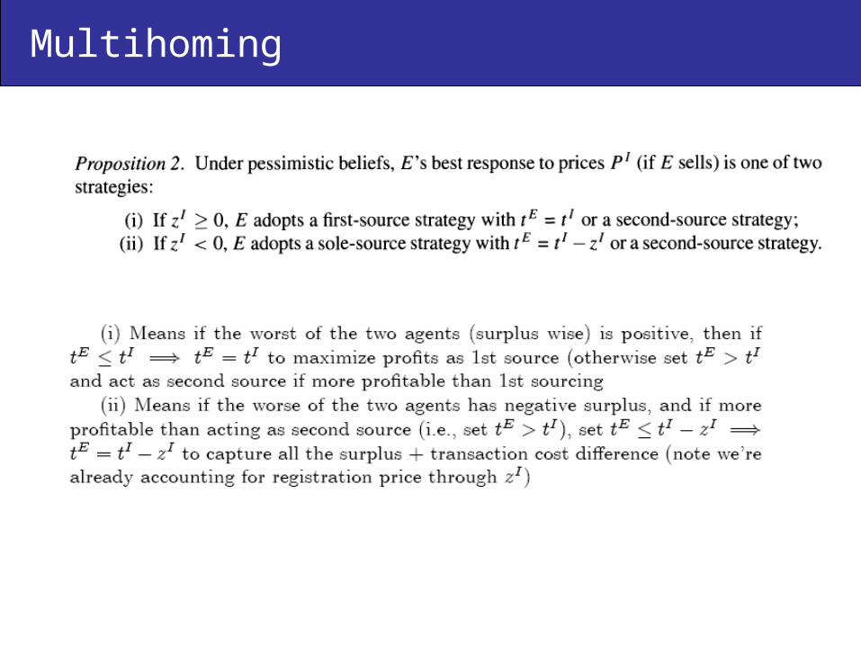
Multihoming

Appendix
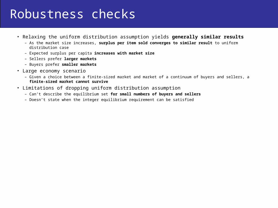
Robustness checks
• Relaxing the uniform distribution assumption yields generally similar results– As the market size increases, surplus per item sold converges to similar result to uniform distribution case
– Expected surplus per capita increases with market size
– Sellers prefer larger markets
– Buyers prefer smaller markets
• Large economy scenario– Given a choice between a finite-sized market and market of a continuum of buyers and sellers, a finite-sized market
cannot survive
• Limitations of dropping uniform distribution assumption– Can’t describe the equilibrium set for small numbers of buyers and sellers
– Doesn’t state when the integer equilibrium requirement can be satisfied
Model extensions
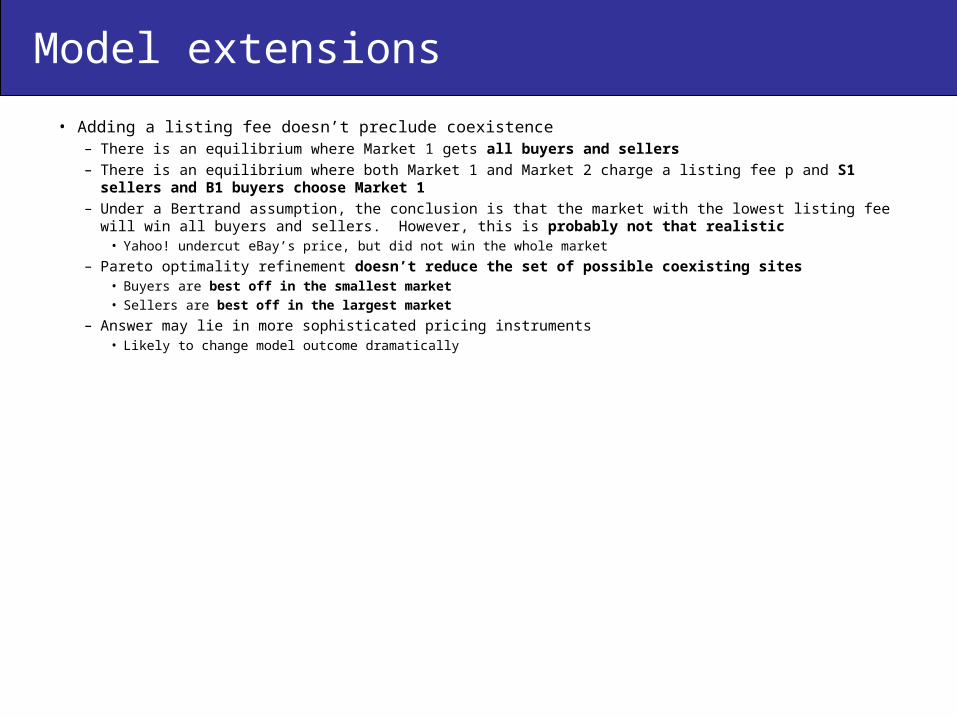
• Adding a listing fee doesn’t preclude coexistence– There is an equilibrium where Market 1 gets all buyers and sellers– There is an equilibrium where both Market 1 and Market 2 charge a listing fee p and S1 sellers and B1 buyers choose
Market 1– Under a Bertrand assumption, the conclusion is that the market with the lowest listing fee will win all buyers and sellers.
However, this is probably not that realistic • Yahoo! undercut eBay’s price, but did not win the whole market
– Pareto optimality refinement doesn’t reduce the set of possible coexisting sites• Buyers are best off in the smallest market
• Sellers are best off in the largest market
– Answer may lie in more sophisticated pricing instruments• Likely to change model outcome dramatically


