Platform Enterprises:

Financing, Investment, and Network Growth

Joanne Juan Chen

London School of Economics ∗

This version: November 2019

Abstract

This paper develops a tractable micro-founded dynamic platform model

featuring cross-group network effects. Networks are analogous to capital-assets,

and the platform enterprise invests in the networks by making subsidies to

users. The paper solves for the entrepreneur’s optimal financing and investment

strategies, with limited enforcement as the major financial friction. The main

results are: 1) making highly aggressive subsidies by using up available funds

is constrained-optimal; 2) per-transaction subsidies decrease over time and

are followed by increasing fees; 3) the platform with stronger network effects

has a propensity to make more subsidies at initial stages and enjoys a higher

valuation; 4) staged financing mitigates the limited enforcement problem, and

ceteris paribus, the number of funding rounds decreases with profitability of

the platform and increases with required profits by financiers; 5) the value of

funds raised each round increases and the financing frequency decreases over

time.

Key words: sharing economy, network effects, platform valuation, dynamic

pricing strategy, subsidy, staged financing

∗I’m grateful to Daniel Ferreira, Martin Oehmke, Mike Burkart, Vicente Cunat, Hongda Zhong,Amil Dasgupta, and seminar participants at LSE for their helpful comments. All errors are theauthor’s responsibility. Contact information: Joanne Juan Chen, Department of Finance, LondonWC2A 2AE, UK. Email: J.Chen64@lse.ac.uk.

1

1 Introduction

Enterprises that leverage the power of platform business models have grown

dramatically in size and scale over the past few years. Prominent examples are Uber,

Airbnb, Upwork, etc., through which services are traded; and Amazon, eBay, Taobao,

etc., where commodities are traded. A platform enterprise doesn’t produce goods by

itself. Instead, it creates networks of users who interact and transact through the

platform and establishes a platform market. Compared with traditional markets, the

platform market is ultimately driven by network effects, which enable the users to

benefit more from trading through the platform when the network size of the other

group is larger. Usually, the platform enterprise charges spreads between the selling

and purchasing prices, and it makes profits from these fees.1

The business model of platforms has attracted attention from both industry and

academia. While there is copious academic work focusing on competition and fee

structure of platforms, studies on the financing and investment of platform enterprises

are sparse. Some interesting questions remain unanswered: is it rational for platforms

to make highly aggressive subsidies to users at early stages, especially when the

platform enterprise is a monopoly with no entry threat? Why does the number of

financing rounds vary greatly for different platform enterprises?2 How would the

capital market conditions affect a platform enterprise’s financing and investment

decisions and its valuation? This paper develops a dynamic theory of platform

financing and investment to study these questions.

The platform financing and investment questions are unique in the following

aspects. First, a platform is an enterprise but it builds up a market. Therefore,

it possesses properties of both a firm and a market. Besides, a platform tends to

allocate a large portion of funds for making subsidies to users, even there is no

competitor or entry threat. So, subsidies cannot be simply regarded as predatory

pricing strategy of the platform enterprise. Instead, subsidies are investment into

the networks, and the networks are analogous to capital-assets, which the platform

enterprise first invests in and later generates income from. The model in this paper

1Fees charged by the platforms can be in different forms. Some platforms directly charge aper-transaction commission from sellers and buyers, e.g. Upwork and Amazon; some set sellingand pricing prices for the users and make profits from the price differences, e.g. Uber. Here,the spread includes both of these forms. Some platforms charge membership fees in addition toper-transaction fees. In the model of this paper, the fixed membership fee is set to zero. Thissimplification assumption does not affect qualitative results.

2For example, Amazon raised two rounds of funding in total, while Uber has raised twenty-threerounds till the end of October 2019, according to data from Crunchbase.

2

captures these distinctive features of a platform and solves for optimal financing

and investment decisions of a monopolistic platform enterprise under various capital

market conditions.

In the model, there is a massive fully-competitive traditional market and a

newly-launched platform market where the same type of good is traded. Network

effects in the platform market generate additional surpluses, which can be shared

by the platform enterprise and the agents. This is the ultimate reason why the

platform enterprise can charge fees on transactions. Once a new agent gets to know

the platform market, he will try it out and decide whether to switch to it from the

traditional market, with an option to switch back. The traditional market is assumed

to be immense and unresponsive to the platform market. The entrepreneurial

platform enterprise has the incentive to make subsidies to users to boost network

growth and maximize its value. With no internal funds, the entrepreneur has to raise

external capital to invest in the networks. Therefore, he needs to decide jointly on

the amount and timing of financing and investment in a world with financial frictions

and financing costs.

The first key finding of the model is that in face of financial constraints, it is

constrained-optimal for the platform to make highly aggressive subsidies by using

up available funds early on. This result highlights the importance of networks as

intangible assets of the platform enterprise. Timely and sufficient investment in

the networks is crucial for the success of a platform.3 Financial constraints are

endogenized in this paper: the entrepreneur may rationally choose not to invest up

to the unconstrained-optimal level because of financing costs. When the financial

constraint is binding, it’s suboptimal to use the funds gradually and smoothly. On

the contrary, it is rational to make heavy subsidies early on and charge zero spread4

subsequently for a certain period.

The model explicitly solves for the (constrained) optimal dynamic pricing strate-

gies of the platform enterprise and the corresponding network growth paths. It finds

that the spread charged by the platform is non-decreasing over time. That is, the

3A prominent example of failure due to inadequate subsidies and slow network growth isSideCar, a ride-sharing company similar to Uber. According to an article on Havard BusinessReview: it deliberately pursued innovation and a conservative slow-growth strategy in order to befinancially responsible. The fatal flaw was not recognizing the importance of attracting both sides ofthe platform. Sidecar also raised much less venture capital than Uber and Lyft, and was unable toattract enough drivers and riders to survive much beyond the startup phase. (Yoffie, Gawer andCusumano, 2019).

4The model assumes a zero maintenance cost for simplicity. Intuitively, the platform may retainsome funds and charge a maintenance-level commission if the maintenance costs are positive.

3

per-transaction subsidies decrease over time and are followed by weakly increasing

fees. The model also predicts that ceteris paribus, stronger network effects, defined

as more user benefits from the same network size, lead to more aggressive subsidies

early on and hence a higher platform valuation and faster network growth.

In terms of financing patterns, this paper argues that staged financing can be a

natural choice to mitigate incentive problems. Intuitively, staging allows the financiers

to abandon the project in case of misconduct, and fewer available funds in hand

reduce the entrepreneur’s incentives of misconduct. The type of potential misconduct

this paper considers is limited enforcement – the entrepreneur could abscond with

funds in hand. This is an extreme case of fund embezzlement, where the entrepreneur

could embezzle all the funds he had just raised. In practice, fund embezzlement is

indeed a severe problem for startups, especially for platform enterprises which need

enormous investment before earning profits.5 This paper finds that, with potential

embezzlement, each round the entrepreneur cannot raise more funds than his expected

profits from successfully managing the platform enterprise. This leads to an increased

value of funds raised each round over time and decreased financing frequency. The

model simultaneously endogenizes the number of rounds, the financing frequency,

and the value of funds raised.

The paper also analyzes how the number of financing rounds is affected by the

profitability of the platform as well as the capital market conditions. All things

equal, higher profitability leads to fewer rounds of financing; a more competitive

capital market leads to fewer rounds of financing. When the capital market is

not fully competitive, the more profits the financiers require, the less investment

the entrepreneur tends to make, and the more rounds of financing he has to raise.

However, an excessively high cost of financing would lead to no financing and

no investment in the networks. This paper characterizes the interaction between

discrete financing choices and continuous investing decisions under different scenarios.

Relation to Literature

Rochet and Tirole (2003, 2006) and Armstrong (2006) provide pioneering work

on platform markets. Their work involves the type of platforms where price non-

5Many failed platform enterprises have been accused of entrepreneur fund embezzlement. Forexample, Kongkonghu, a platform trading second-hand goods in China, was reported the CEOembezzlement of funds for private usage. In this paper, I assume that fund embezzlement can bedetected before the next round of financing, because of investors’ monitoring efforts or due diligenceundertaken before each new round of financing.

4

neutrality of the two sides is a key feature. They define the platform markets with this

non-neutral price structure as two-sided markets. Rochet and Tirole (2006) summarize

that factors making a market two-sided are: absence or limits on the bilateral pricing

setting, platform-imposed constraints on pricing and membership fixed costs or fixed

fees. Examples of those markets are credit card markets, newspapers, Videogame

platforms, etc. Rochet and Tirole (2003, 2006) and Armstrong (2006) develop

static models on the two-sided markets to discuss competition and price structure of

platforms in various cases. This paper, in contrast, involves platforms which either

allow bilateral pricing by end-users (e.g. Amazon, Deliveroo, Upwork, etc.) or charge

no membership fees and optimally set prices satisfying the market clearing condition

to maximize profits (e.g. Uber). Thus, in this paper, equilibrium transaction amounts

and prices are endogenously determined by market clearing, and only the level of fees

charged by the platform matters in equilibrium. This simple price structure allows

me to explore the dynamics of the platform and find closed-form expressions. To my

knowledge, this paper provides the first attempt to describe the optimal dynamic

pricing strategy and network growth path of the platform market based on a fully

micro-founded model.

Another strand of literature studies competition with same-side network effects,

following the work by Katz and Shapiro (1985), and Farrell and Saloner (1985, 1986).

Some more recent work of this literature addresses the issue of dynamic competition

and growth. Mitchell and Skrzypacz (2006) derive the Markov perfect equilibrium of

an infinite-period game with network effects. They assume the consumer’s utility to

be an increasing function of the network size at the time of trade. I make similar

assumptions in this paper. That is, the agents are assumed to be myopic and not

forward looking. Cabral (2011) considers dynamic pricing competition between two

proprietary networks with forward-looking agents. My work is distinguished from

this strand of literature in the following aspects. First, I model the cross-group

network effects of the platform market. Second, I focus on the effect of network

itself on the dynamic pricing decisions without competition or entry threat. Third, I

introduce financial frictions in the model and study the joint decisions of dynamic

financing and pricing. The topic on dynamic platform competition and its interaction

with financing issues is a good direction for future research.

For the financing part, this paper is related to the literature on venture capital

(VC) staging. Admati and Pfleiderer (1994) model the staging as a way to mitigate

agency problems such as asymmetric information and overinvestment. Wang and

5

Zhou (2004) investigate the cases with moral hazard and uncertainty and find that

staged financing can control risk and mitigate moral hazard. Most work on VC

staging has assumed either fixed investment levels or a fixed number of stages. This

paper endogenizes the financing and investment levels, the number of stages, and

frequency of financing simultaneously, without resort to uncertainty.

This paper is also related to work on continuous-time models of the firm’s financing

and investment decisions and the impact of external financing costs on investment.

Decamps et al. (2011) explore a model where a firm has a fixed-size investment

project and generate random cash flows, and they study the impact of external

financing costs on equity issuance and stock prices. Bolton, Chen, and Wang (2011)

study the case of flexible firm size and the dynamic patterns of corporate investment.

Demarzo et al. (2012) study the dynamic investment theory with dynamic optimal

incentive contracting, and endogenize financial constraints. Section 3 of this paper

also endogenizes financial constraints, but this paper involves no uncertainty. Limited

enforcement along with financing costs leads to endogenous financing level, staging,

and pricing decisions in this paper. Besides, the literature consider either fixed-size

investment or AK production technology, while this paper endogenizes the cash flows

by modelling the unique business patterns of the platform enterprise.

The remainder of this paper proceeds as follows. Section 2 sets up and solves

for the framework of the dynamics of the platform market, and compares it with

the traditional markets and firms. Section 3 discusses the financing and investment

issues with financial frictions, and characterizes the constrained-optimal financing

and investment patterns. Section 4 concludes. Proofs appear in the Appendix.

2 Framework of the Platform Market

To understand the strategies of the platform enterprise, we first need to know

how the platform market works. In this section, I build a framework to analyze the

dynamics of the platform market, and the corresponding pricing strategies of the

platform enterprise.

The investment strategy of the entrepreneur who runs the platform enterprise

is highlighted in this section, assuming no financial frictions or financing costs, or

equivalently, the entrepreneur has sufficient internal funds to make the investment.

6

Discussion for financial frictions and the interaction between financing and investment

decisions are deferred until next section.

2.1 The Model

Time is continuous and the discount rate in this economy is r > 0.

In this economy, there is a massive fully-competitive traditional market trading

one good, with no network effects. All agents originally trade in this traditional

market. At time t = 0, a monopolistic platform is launched by an entrepreneur to

trade the same good. The platform enterprise creates networks of users, which in

turn generate network effects. The initial network size is normalized to be one on

each side of the platform market. An agent can switch frictionlessly between the

traditional market and the platform market once he gets to know both. Hence, a

user of the platform always compares the utility gained from trading in the platform

market with his reservation utility when trading in the traditional market, and

decides whether to stay in or exit the platform market. There is a fixed cost F0 to

launch the platform, which can be ignored in this section, since it is a sunk cost and

does not affect the entrepreneur’s investment decisions thereafter.

The information of the platform market is disseminated in the economy by “word

of mouth”: current users of the platform will constantly tell his or her friends of it.

An agent who has just heard of the platform market will transact one unit of the

good and compare the utility with his corresponding reservation utility to decide

whether to switch to the platform market. To simplify the analysis, I assume there

is no cost to commence, keep, or terminate the platform membership. The platform

generates profits by charging spreads between the purchasing and selling prices. The

platform’s objective is to maximize all discounted future profits.

The remainder of Subsection 2.1 set up the model in details. Part A describes

the instantaneous utilities of platform users; Part B then solves for the instantaneous

supply and demand functions of the platform market and the market-clearing equi-

librium; Part C introduces the law of motion of the platform market; Part D defines

the problem of the platform.

7

A. Instantaneous Utilities of Platform Users

The good is indivisible. On each side of the market, agents are homogeneous.

Their utilities are assumed to be quasilinear. A buyer has the standard decreasing

marginal utility and a seller experiences an increasing marginal cost. A key setup

factor in this model is the cross-group network effects in agents’ utilities when trading

through the platform. That is, the net utility of an agent not only depends on the

amount of goods/services he consumes or sells, but is also related to the network

size of the group on the other side of the market.

The utility UD of a buyer on the demand side and the utility US of a seller on

the supply side are, respectively,

UD(xD) =

∫ xD

0

(b1 + εi −N−ηS x)dx− pDxD, (1)

US(xS) = pSxS −∫ xS

0

(b2 + εi +N−ηD x)dx. (2)

For a buyer, the term (b1 + εi −N−ηS x) is the utility he gains from consuming an

infinitesimal unit of the good at consumption level x. b1 denotes the average product

quality. The zero-mean random variable εi is an identical and mutually independent

shock component in the quality of each infinitesimal unit of the good, where i is

an index for the ordinal value of the units. −N−ηS x exhibits a decreasing marginal

utility. The component N−ηS represents the cross-group network effect, where η is a

non-negative parameter representing the strength of the network effect.6 pD is the

per-unit purchasing price of the good, and xD is the level of consumption.

The above setting assumes that the cross-group network size directly affects the

pace of decline in the marginal utility, but not the quality of the good. This is

a novel way of specifying network effects. It is a reasonable assumption because

the benefits of cross-group network effects usually hail from product variety, lower

searching costs or better matching results, which slow down the decrease in the

agent’s marginal utility rather than affecting the quality of the good. For example, a

buyer on Amazon enjoys slower utility decrease if there are more sellers and thus

product differentiation; the utility of a Uber-rider also decreases more slowly if there

are more drivers and hence higher matching frequency. More broadly, network effects

6When η = 0, there is no network effect. As will be shown later, the platform can never chargea positive commission in this case, so the optimal choice is not to launch the platform if there is nonetwork effect.

8

can be understood as benefits of convenience generated by the platform market,

which do not exist in the traditional market – to purchase more differentiated goods,

the potential buyer has to go to different stores in the traditional market; to take

more rides, the traveller has to book taxis several more times and wait longer in the

traditional market; while with platforms like Amazon and Uber, they don’t have

to. Thus, users of the platform tend to experience a slower decrease in the marginal

utility and potentially consume more.

A seller’s utility is the profits he gets from selling xS units of the good, since his

utility is also quasilinear. pS is the selling price of the good. pS may be different

from pD because the platform can charge a spread between these two prices. This

spread can be either positive or negative. The term (b2 + εi +N−ηD x) is the cost of

providing an infinitesimal unit of the good at level x. Similar to the demand side, εi

is a shock in the cost of each infinitesimal unit of good produced, N−ηD x demonstrates

the increasing marginal cost, and N−ηD measures the cross-group network effect.

The larger the network size of the demand side, the more slowly the marginal cost

increases. This setting is most suitable for the suppliers in the “sharing economy” or

“gig economy”, where the economies of scales generally do not apply to an individual

supplier, and they encounter increasing marginal costs. For example, a freelancer of

Upwork or a room-provider of Airbnb usually experience increasing marginal costs

from more work or longer waiting time in between, but the larger network size of

the demand side can mitigate the increase.

In this model, I assume εi ∼ U [− b2, b

2], i.i.d., where b = b1−b2. More explanations

of this assumption will be given in Section 2.1.C.

Integrate (1) and (2), and by the law of large numbers, the agents’ utilities are in

the quadratic quasilinear form:

UD(xD) = (b1xD −1

2N−ηS x2

D)− pDxD, (3)

US(xS) = pSxS − (b2xS +1

2N−ηD x2

S). (4)

B. Demand, Supply, and Platform Market Equilibrium

Knowing agents’ utilities, we can solve for the demand and supply functions as

well as the market equilibrium, taken the spread charged by the platform as given.7

7In the model, I assume the platform will impose the market-clearing equilibrium instead ofrationing equilibrium, because the former maximizes the platform’s profits and also generates the

9

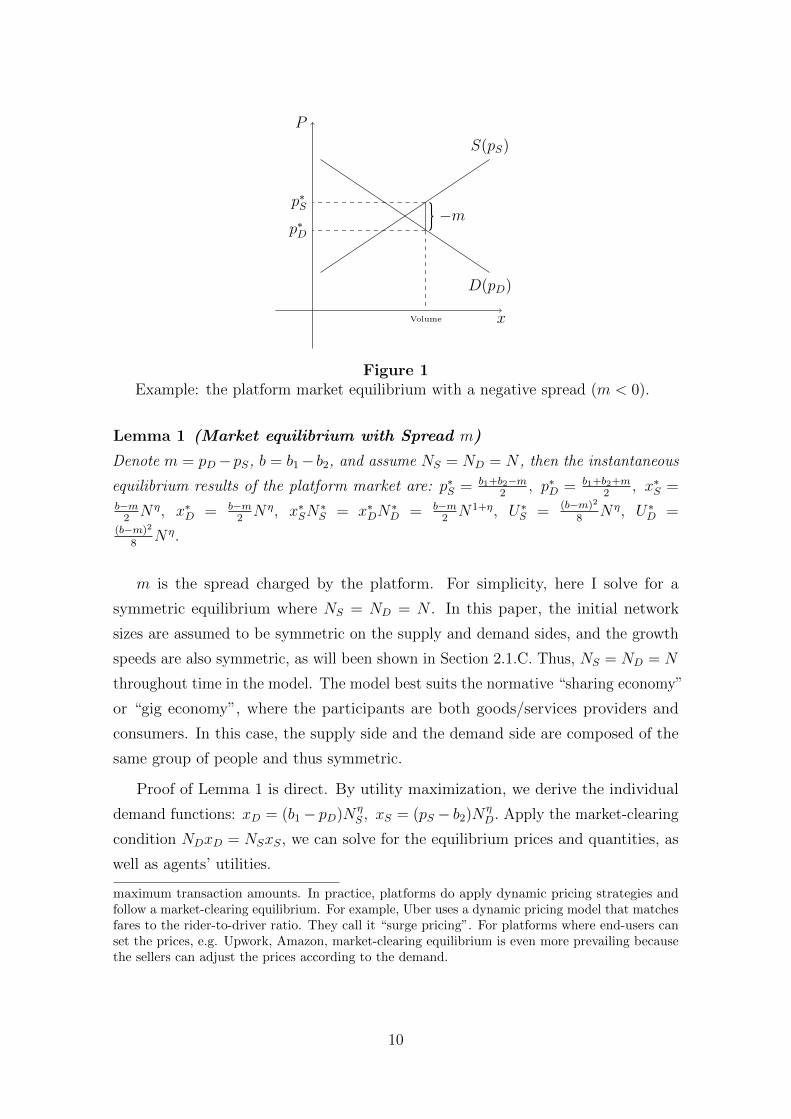
x

P

D(pD)

S(pS)

−m

Volume

p∗S

p∗D

Figure 1Example: the platform market equilibrium with a negative spread (m < 0).

Lemma 1 (Market equilibrium with Spread m)

Denote m = pD−pS, b = b1− b2, and assume NS = ND = N , then the instantaneous

equilibrium results of the platform market are: p∗S = b1+b2−m2

, p∗D = b1+b2+m2

, x∗S =b−m

2Nη, x∗D = b−m

2Nη, x∗SN

∗S = x∗DN

∗D = b−m

2N1+η, U∗S = (b−m)2

8Nη, U∗D =

(b−m)2

8Nη.

m is the spread charged by the platform. For simplicity, here I solve for a

symmetric equilibrium where NS = ND = N . In this paper, the initial network

sizes are assumed to be symmetric on the supply and demand sides, and the growth

speeds are also symmetric, as will been shown in Section 2.1.C. Thus, NS = ND = N

throughout time in the model. The model best suits the normative “sharing economy”

or “gig economy”, where the participants are both goods/services providers and

consumers. In this case, the supply side and the demand side are composed of the

same group of people and thus symmetric.

Proof of Lemma 1 is direct. By utility maximization, we derive the individual

demand functions: xD = (b1− pD)NηS , xS = (pS − b2)Nη

D. Apply the market-clearing

condition NDxD = NSxS, we can solve for the equilibrium prices and quantities, as

well as agents’ utilities.

maximum transaction amounts. In practice, platforms do apply dynamic pricing strategies andfollow a market-clearing equilibrium. For example, Uber uses a dynamic pricing model that matchesfares to the rider-to-driver ratio. They call it “surge pricing”. For platforms where end-users canset the prices, e.g. Upwork, Amazon, market-clearing equilibrium is even more prevailing becausethe sellers can adjust the prices according to the demand.

10

Figure 1 depicts the market demand function, D(pD) = (b1 − pD)NηSND, the

market supply function, S(pS) = (pS − b2)NηDNS, and the equilibrium prices and

trading volumes under a negative spread m. With a negative m, the trading volume

is stimulated and agents trade more because of the subsidies. If instead m is positive,

the platform makes profits and the equilibrium trading volume is lower than the

zero-spread volume.

C. Law of Motion of the Platform Market

The law of motion guarantees how this platform market dynamically evolves. It

consists of three parts - dissemination of news, the joining decision of a newcomer,

and exit decision of an existing user.

To understand the joining and exit decisions of the agents, we need to know their

outside opportunities. In this economy, there is a traditional competitive market

trading the same good with the same quality, but with no network effects. Agents

can always trade in this traditional market. The selling and purchasing prices are

equal in the traditional market. Thus, utility parameters b1 and b2 remain the same

in the traditional market; with no network effects, η = 0; with no price difference,

pS = pD = p. Namely, agents’ instantaneous utilities in the traditional market are:

UD(xD) = (b1xD −1

2x2D)− p · xD, US(xS) = p · xS − (b2xS +

1

2x2S). (5)

Therefore, the equilibrium price of the traditional market is p∗ = b1+b22

, and the

equilibrium utility of a buyer or seller is U∗R = b2

8.

For the dissemination of news on the platform market, assume a member of the

platform tells λ fraction of his friends about the platform each unit of time. That

means, the arrival rate of newcomers on each side is λN .

A newly arrived agent will choose to “have a taste” of the network to gather

information. To be specific, his decision rule is as follows: trade an infinitesimal

unit of the good through this platform and compare the utility gained with the

corresponding reservation utility in the traditional market. The latter is b/2. 8

8It is actually the marginal utility at x = 0 in the traditional market, which can be derived from(5). There is no shock to the quality in the traditional market, because the buyers and sellers usuallymeet and examine the goods before the transaction is made. In the platform market, however,transactions are usually made before or even without personal contact between a buyer and a seller,which leads to shocks in the realization of the costs and the good quality.

11

If he gains a higher utility than the corresponding reservation utility, he will join

the network and switch from the traditional market to the platform market. With

some abuse of notation, I denote the utility from trading an infinitesimal unit in the

platform market by the marginal utility, MU :

MUD|x=0 = (b1 + εi)− pD =b−m

2+ εi, (6)

MUS|x=0 = pS − (b2 − εi) =b−m

2+ εi. (7)

Therefore, the probability of a newcomer to join the network is

Pr(b−m

2+ εi >

b

2) = Pr(εi >

m

2) =

b−m2b

, (8)

because we have assumed that εi ∼ U [− b2, b

2], i.i.d. in Section 2.1.A.

Once joining the platform market, the user will optimally choose to trade the

equilibrium amount as shown in Lemma 1. If the utility he gets is lower than the

equilibrium reservation utility in the traditional market, U∗R = b2

8, he will immediately

exit the platform. Because agents are homogeneous, the platform would collapse in

this case. So, the platform will always guarantee U∗S = U∗D > U∗R, i.e. (b−m)2Nη > b2.

I name this constraint “no-exit condition”.

Combining all the three parts above, and assuming the potential size of the

platform market is N , the law of motion for each side of the platform market is 9

N =

λ

2b(b−m)N, if N < N,

0, if N = N,

(9)

where m and N must always satisfy the no-exit condition: (b−m)2Nη > b2.

D. Problem of the Entrepreneur

In Section 2, I assume the entrepreneur who runs the platform enterprise is

financially unconstrained. Therefore, his objective is to maximize the discounted

9For the law of motion in (9) to hold, m ∈ [−b, b], because the probability b−m2b ∈ [−1, 1]. The

upper bound never binds since the static monopolistic price is b2 ; the lower bound may bind. In this

paper, I only consider the set of parameters {η, λ, r, N} where the lower bound of m does not bind,which is realistic, since platforms in general will not make extreme subsidies. Even if this lowerbound binds, it won’t affect the qualitative results of this paper, but only generates a segment of(−b) level of m at initial stages of a platform’s dynamic pricing strategy.

12

cash flows generated by the platform enterprise, subject to the law of motion and

the no-exit condition:

maxm(t)

∫ ∞0

e−rtm(t)[b−m(t)]

2N(t)(1+η) dt

s.t. N(t) =

λ

2b[b−m(t)]N(t), if N(t) < N,

0, if N(t) = N,

& [b−m(t)]2N(t)η > b2, ∀t.

(P1)

2.2 Model Solutions and Analysis

In this subsection, I present the closed-form solutions for the entrepreneur’s

problem (P1). Problem (P1) is a standard dynamic optimization problem, with m(t)

as the choice variable and N(t) as the state variable. Denote the optimal policy

function by m∗(t) and the corresponding optimal state function by N∗(t). Denote

value function by Πm∗(t). 10 Then the optimized objective function in Problem (P1)

is Πm∗(0).

We know that the static monopolistic price is b2. Here, I first show that if the

platform can indeed charge this monopolistic price when the network reaches the

maximum size N , and the optimal strategy is indeed to make subsidies at the very

beginning (m∗(0) < 0), then the no-exit constraint will never bind all along the

optimal path. Put differently, if the no-exit constraint does not bind on the initial

point and the endpoint, then it does not bind on the whole path.

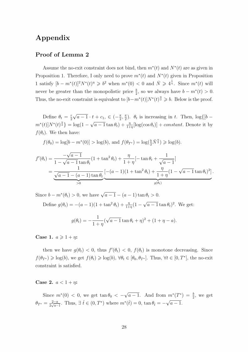
Lemma 2 If m∗(0) < 0 and N > 41η , the no-exit constraint [b−m(t)]2N(t)η > b2

will not bind on the optimal path.

Proof of Lemma 2 is in Appendix. In this paper, I will only consider the cases

where m∗(0) < 0, because this paper focuses on the discussion of the optimal

investment strategy and its interaction with financing decisions. Besides, as will be

shown later, the cases where the platform optimally makes no investment at the very

beginning (m∗(0) > 0) are less profitable cases. With a high launch cost F0, these

cases are naturally ruled out because the profits of the platform enterprise are not

enough to cover the launch costs.

10The value function can also be expressed as a function of the state variable, i.e. Πm∗(t) =

Π(N∗(t)).

13

The closed-form solutions of the entrepreneur’s problem (P1) is presented in

Proposition 1. Please see Appendix for detailed derivation and proof.

Proposition 1 (Solutions to P1)

Let λ(1+η)2r

= a > 1, and N > 41η . The optimal policy function m∗(t), network growth

N∗(t), and discounted future profits Πm∗(t), are as follows:

m∗(t) =

b

a

√a− 1 tan(

r

2

√a− 1 · t+ c1) +

b

a(a− 1) , if t < T ∗

b/2 , if t > T ∗

N∗(t) =

er

1+ηt+c2 · [cos(

r

2

√a− 1 · t+ c1)]

21+η , if t < T ∗

N , if t > T ∗

Πm∗(t) =

1

2rN∗(t)(1+η)[b−m∗(t)]2,

if c1 < arctan(−√a− 1). The exogenous parameters are (b, r, η, λ, N). Constants c1

and c2, and the market growth termination time T ∗ are determined by the end points:

N∗(0) = 1, N∗(T ∗) = N , m∗(T ∗) = b2.

The exogenous parameters b and r are properties of the economy, and η, λ, and

N are specific for the platform enterprise. Here, the inequality c1 < arctan(−√a− 1)

guarantees that the optimal strategy of the platform is indeed to make investment

(subsidies) at initial stages; Restriction on the potential market size, N > 41η ,

guarantees the platform can charge the monopolistic price b2, when the market

reaches its maximum size. For the range of a, I will show in Appendix that if a 6 1,

m∗(0) > 0. Therefore, this paper focuses on a > 1. A visual example of Proposition

1 is given in Figure 2.

Remark 1.1 The optimal pricing strategy m∗(t) is monotonically increasing.

Remark 1.1 emphasizes that it is efficient for the platform to make subsidies

early on and charge a commission later. It is never optimal to undulate this spread,

switching between subsidies and commission. As will be shown in Section 3, this

monotone-increasing property of the pricing strategy holds in more general cases

with financial frictions.

Remark 1.2 Let the economy has constant r and b. Then for the platform enterprise,

a stronger network effect η, a faster information dissemination speed λ, or a large

14

maximum potential network size N , will result in more subsidies at initial stages,

and meanwhile, a higher valuation of the platform.

Remark 1.2 predicts that with constant r and b, if we observe that a platform

makes heavier subsidies at initial stages, then it tends to enjoy a higher valuation.

This result can be got directly from Proposition 1 by plugging t = 0 into Πm∗(t):

Πm∗(0) = [b−m∗(0)]2

2r. That is, a more negative m∗(0) leads to a higher Πm∗

(0). Besides,

since a higher η, λ, or N leads to a higher valuation of the platform, 11 each of them

must lead to more subsidies at the beginning.

Figure 2 depicts how m∗(t), N∗(t) and Πm∗(t) evolve over time, and also flows of

investment (subsidies) in the time-zero value.12 This example demonstrates that a

stronger network effect leads to a steeper optimal pricing path, faster network growth,

and a higher platform value. Here, Πm∗(0) = 15.68 if η = 1, and Πm∗

(0) = 8.35

if η = 0.9. Figure 2(D) shows that the time-zero value of investment flows keep

decreasing over time in this example.

A. Comparison with the Traditional Market

The main distinction between the platform market and the traditional market is

the existence of cross-group network effects in the former.

Take Deliveroo as an example. It is a British online food ordering and delivering

platform linking the restaurants and the consumers. Consumers can order online

from a wide range of restaurants which may not be within walking distance, and

wait at home for the food to be delivered. The traditional market counterpart is the

decentralized local restaurant market. Through Deliveroo, consumers have access

to a large group of restaurants. Hence, they tend to consume more because of the

richer product variety brought by the platform, compared to limited choices of local

restaurants near home. Deliveroo charges a commission from the restaurant which

in turn affects the prices of food listed on the platform by the restaurants. The story

is similar for Amazon. Uber is also similar if we regard the traditional market as the

taxi-booking market. 13

11A heuristic proof is as follows. With higher λ, keep the path for N(t) the same as before.Then the new path m(t) > m∗(t) ∀t, which results a higher Π(0). With higher η, keep the path forN(t)(1+η) as before, and this leads to a higher m(t) and higher instantaneous profits for all t, thusa higher Π(0). With a higher N , keeping the original path can lead to a higher Π(0).

12The expression is e−rt m(t)[m(t)−b]2 N(t)(1+η).

13In many cities’ taxi market, customers must book in advance for a taxi, which exhibits nonetwork effect.

15

Figure 2Parameters: b = 1, r = 0.1, λ = 0.12, N = e5, η = 0.9 or 1.

The network effects are indispensable for a platform enterprise to exist and make

profits. If on the contrary, the platform contains no network effects, i.e. η = 0, then

the platform is exactly the same as the traditional market and it can never charge

a commission. Once the platform charges a positive spread, the no-exit condition

[b−m(t)]2N(t)η > b2 immediately breaks and all agents exit. Intuitively, when the

platform brings no additional surplus to agents compared with the traditional market,

there is no room for it to charge a commission. Thus, ex ante the entrepreneur has

no incentive to launch the platform if there are no network effects in this market. If

the network effects are weak, the commission that can be charged by the platform

is low and it leads to low profitability of the platform enterprise. With some fixed

launch costs or flow maintenance costs, the platform enterprise cannot survive either.

B. Comparison with the Traditional Production Firms

Perhaps surprisingly, the optimal behavior of a platform enterprise exhibits

similarities to a traditional production firm. They both invest first and profit later.

The networks of the platform are analogous to the capital assets of a production

firm. The platform first invests in the networks and then extract profits from the

16

networks. Therefore, the platform generates negative cash flows early on and positive

cash flows later, which has a similar pattern to a traditional production firm.

Some characters of the platform enterprise’s investment this paper would like

to emphasize and which may be different from a traditional production firm are

as follows. 1) The optimal investment-stage and production-stage of the platform

enterprise are clearly separated. The entrepreneur running the platform enterprise

has the choice to switch between investment (subsidy) and production (commission)

as frequently as he wishes, but he will never do so because it’s suboptimal. 2) The

investment for a platform enterprise takes place dynamically and gradually and a

perfect timing is extremely important. Once the platform cannot follow the optimal

timing, it will suffer from slower growth and a lower valuation. 3) There is no

depreciation in the network, unlike most capital assets in production firms. Once

the network is built, it lasts forever unless the agents exit.

If the entrepreneur does not have adequate internal funds to make investment,

he has to raise external funds. Section 3 discusses the entrepreneur’s financing issues

in detail.

3 Financing Under Limited Enforcement

Section 2 builds up a dynamic model for the platform business. The optimal

investment and pricing strategies of the entrepreneur are studied, assuming he is

financially unconstrained. What if the entrepreneur needs to raise external financing

and there exist financial frictions and financing costs, as are common to start-up

firms? In this section, I analyze the financing and investment strategies of the

entrepreneur when there exist financial frictions and financing costs. Moreover,

to analyze the influences of financial market conditions, I relax the assumption

of a fully-competitive capital market. Financiers may require positive profits for

their investment. I examine how the required profits affect the incentives of the

entrepreneur and thus his financing level, staging, and timing choices.

17

3.1 The Model

The type of financial friction I consider in this paper is limited enforcement,

which constrains the entrepreneur’s ability to make credible promises.14 I assume

the enforcement of contracts is limited as follows: the entrepreneur can abscond

with funds in hand, instead of investing the funds in the networks. The entrepreneur

has the incentive to abscond with funds once he has more funds in hand than what

he expects to get from successfully managing the platform enterprise. The profits

generated by the platform are assumed to be verifiable and paid out as dividends

straight away. Thus, the entrepreneur can potentially embezzle the funds but not

the operational cash inflows.

Specifically, the setting of the model is as follows: The platform enterprise is

launched by an entrepreneur, who has skills but no money. There is a fixed cost F0 to

launch the platform enterprise, and any other costs for operating the platform are set

to zero. The fixed cost has already been covered through the “angel investment” (or

initial rounds of financing), and the entrepreneur is obliged to pay back F (time-zero

value) to the angel investors. To invest in the networks, the entrepreneur has to raise

additional financing. Assume that there exists a fixed financing cost C (time-zero

value) for each round of financing. This fixed financing cost is a deadweight loss for

raising a new round of capital, which can be understood as fees paid to the third

parties for project valuation, endorsement, etc. So, each round the entrepreneur raises

(Ij + C) from financier j, where Ij (time-zero value) is invested into the networks.

Financier j requires Wj (time-zero value) as investment profits. That is, he requires

a time-zero value (Ij + C +Wj) back for this investment, where Wj > 0.15

Denote the total number of financing rounds by n. Let W =∑n

j=1Wj, rep-

resenting the aggregate time-zero value of profits required by all financiers, and

I =∑n

j=1 Ij, representing the aggregate time-zero value of funds invested in the

networks. Besides, the model allows the entrepreneur to choose the timing of each

new round of financing. Therefore, he is able to allocate the funds optimally through

time into the networks. That is to say, only the aggregate fund level I, but not any

individual level Ij, affects the optimal investment strategy and the valuation of the

platform.

14Some previous papers consider limited enforcement as a type of financial frictions are Chienand Lustig (2009), Rampini and Viswanathan (2010).

15For simplicity of the problem, all the values in this section are denoted using the time-zerovalue.

18

Let Π0(I) denote the optimized time-zero value of all discounted profits as a

function of I. Π0(I) can be regarded as the solution to a lump-sum constrained opti-

mization problem when the lump-sum investment level is I. Each Π0(I) corresponds

to a unique pricing strategy and network growth trajectory, as will be demonstrated

in Proposition 2 below. Intuitively, Π0(I) increases in I when I 6 I∗, where I∗ is the

optimal time-zero value of investment derived in Section 2,16 and Π0(I∗) = Πm∗(0).

In this model, the aggregate investment level I is endogenously chosen by the

entrepreneur. To be exact, the amount of funds raised each round Ij, and the

number of rounds n, are all endogenously determined by the entrepreneur’s profit-

maximization objective, subject to the incentive compatibility constraint for him not

to embezzle funds and abscond, as well as the individual rationality constraint for

him to launch the platform enterprise and raise external financing to invest in the

networks.

The problem of the entrepreneur is summarized as follows:

maxn,I1,I2,...,In

Π0(I)− F − nC −W

s.t. Π0(I)− F − nC −W > I1 (IC1)

...

Π0(I)− F − nC −W > In (ICn)

Π0(I)− F − nC −W > max{Π0(0)− F, 0} (IR)

where I =n∑j=1

Ij, W =n∑j=1

Wj,

(P2)

and Π0(I) is the solution to the following problem:

maxm(t)

∫ ∞0

e−rtm(t)[b−m(t)]

2N(t)(1+η) dt

s.t. N(t) =

λ

2b[b−m(t)]N(t), if N(t) < N,

0, if N(t) = N,

& [b−m(t)]2N(t)η > b2, ∀t,

&

∫ t

0

e−rxm(x)[m(x)− b]

2N(x)(1+η) dx 6 I, ∀t.

16I∗ =∫ τ∗

0e−rt m

∗(t)[m∗(t)−b]2 N∗(t)(1+η)dt, where τ∗ is the time point when the platform charges

zero spread, or m∗(τ∗) = 0. The entrepreneur will rationally raise I 6 I∗.

19

The entrepreneur maximizes the time-zero value of his expected profits from

optimally and successfully managing the platform enterprise, subject to the incentive

compatibility (IC) constraints and the individual rationality (IR) constraint. The

incentive compatibility constraints say that the funds the entrepreneur receives each

round should be no more than what he expects to gain from managing the platform

enterprise. Otherwise, he would abscond with funds. The individual rationality

constraint says that if the entrepreneur expects to get too little from raising funds

and optimally investing in the networks, he would instead choose not to make the

investment or not to launch the platform enterprise, ex ante.

3.2 Model Solutions and Analysis

To solve Problem (P2), we need to solve for Π0(I) first. As is defined, Π0(I) is

the optimized time-zero value of all discounted future profits of the platform, with

the constraint that the investment level is I. We can solve for the constraint-optimal

pricing strategy m(t) and the network growth function N(t) to get Π0(I). A detailed

derivation of Π0(I) is given in Proof of Proposition 2 in Appendix.

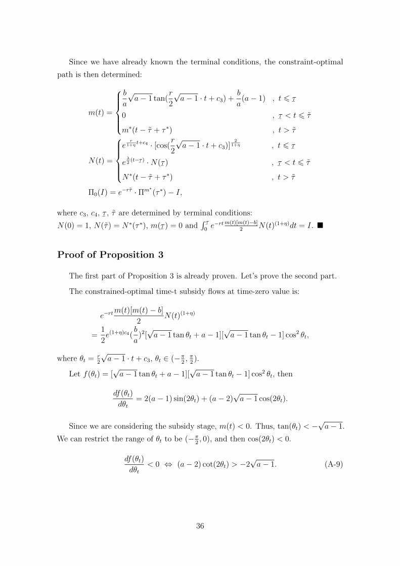
Lemma 3 The constraint-optimal pricing strategy m(t) is non-decreasing.

Lemma 3 shows that the platform’s subsidy stages and commission stages are

clearly divided. It is inefficient to charge a commission for a period and use the

profits as internal funds to make subsidies. Therefore, the platform will never swing

between subsidies and commission. The proof of Lemma 3 may be found in Appendix.

Equipped with Lemma 3, we can solve for m(t), N(t), and Π0(I). The results are

provided in Proposition 2.

Proposition 2 Let a > 1 and N > 41η . Define τ ∗ as the time point when the un-

constrained optimal spread is zero, or m∗(τ ∗) = 0; define I∗ as the optimal aggregate

subsidy amount, or I∗ =∫ τ∗

0e−rt m

∗(t)[m∗(t)−b]2

N∗(t)(1+η)dt. When the available aggre-

gate subsidy amount I 6 I∗, the constraint-optimal policy function m(t), network

20

growth N(t), and the time-zero value of discounted future profits Π0(I), are as follows:

m(t) =

b

a

√a− 1 tan(

r

2

√a− 1 · t+ c3) +

b

a(a− 1) , t 6

¯τ

0 ,¯τ < t 6 τ

m∗(t− τ + τ ∗) , t > τ

N(t) =

e

r1+η

t+c4 · [cos(r

2

√a− 1 · t+ c3)]

21+η , t 6

¯τ

eλ2

(t−¯τ) ·N(

¯τ) ,

¯τ < t 6 τ

N∗(t− τ + τ ∗) , t > τ

Π0(I) = e−rτ · Πm∗(τ ∗)− I,

where c3, c4,¯τ , τ are determined by terminal conditions:

N(0) = 1, N(τ) = N∗(τ ∗), m(¯τ) = 0 and

∫¯τ

0e−rt m(t)[m(t)−b]

2N(t)(1+η)dt = I.

Remark 2.1 When the aggregate amount of available funds is less than the optimal

amount, it is constraint-optimal for the platform to make highly aggressive subsidies

early on and use up the available funds, and then wait with zero spread until it’s

optimal to start to charge a commission.

The results highlight the importance of building up the networks at early stages.

Timely and sufficient investment in the networks is crucial for the success and high

valuation of a platform enterprise. If the entrepreneur misses the best timing to

make investment, the platform enterprise will suffer from a lower valuation or even

failure to survive. A prominent example is the failure of SideCar, as mentioned in

the introduction of this paper. Therefore, it is rational for the entrepreneur running

the platform to use up available funds to make heavy subsidies early on.

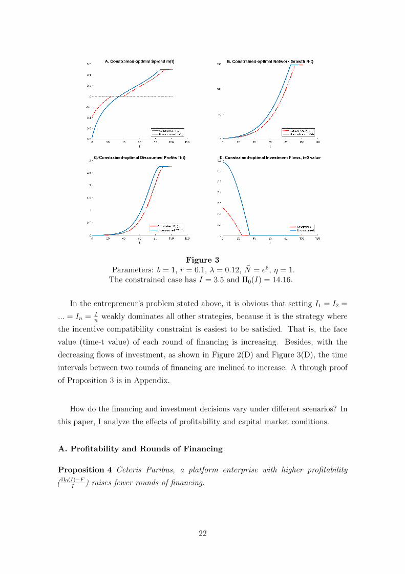
Figure 3 plots an example of constrained-optimal pricing strategy, network growth

pattern, the value of discounted profits, and investment flows, compared with the

unconstrained benchmarks the same as in Figure 2.

Having got Π0(I), I now set out to characterize the solutions for the entrepreneur’s

problem (P2). First, the entrepreneur’s optimal financing patterns are summarized

in Proposition 3.

Proposition 3 Each round of financing has the same time-zero value. Thus, the face

value (time-t value) of the funds raised each round keeps increasing. The frequency

of new rounds keeps decreasing in most of the economically meaningful cases, where

a sufficient condition is a > 54, and N < N∗ such that m(0) > −b.

21

Figure 3Parameters: b = 1, r = 0.1, λ = 0.12, N = e5, η = 1.

The constrained case has I = 3.5 and Π0(I) = 14.16.

In the entrepreneur’s problem stated above, it is obvious that setting I1 = I2 =

... = In = In

weakly dominates all other strategies, because it is the strategy where

the incentive compatibility constraint is easiest to be satisfied. That is, the face

value (time-t value) of each round of financing is increasing. Besides, with the

decreasing flows of investment, as shown in Figure 2(D) and Figure 3(D), the time

intervals between two rounds of financing are inclined to increase. A through proof

of Proposition 3 is in Appendix.

How do the financing and investment decisions vary under different scenarios? In

this paper, I analyze the effects of profitability and capital market conditions.

A. Profitability and Rounds of Financing

Proposition 4 Ceteris Paribus, a platform enterprise with higher profitability

(Π0(I)−FI

) raises fewer rounds of financing.

22

This proposition seems counter-intuitive, but it is actually a general result when

the major financial friction is limited enforcement. All things equal, the more

profitable the enterprise, the more profits left to the entrepreneur. Hence, he can

credibly raise more funds within each round, which leads to fewer rounds of financing.

Proof of Proposition 4 is simple and direct. Using results in Proposition 3, we can

rewrite the incentive compatibility constraints as: Π0(I)−FI

> nCI

+ 1n

+ WI

. Higher

profitability makes the (IC) constraints easier to be satisfied, and thus leads to a

smaller n required, so as to maximize the entrepreneur’s profits.

B. Influences of Capital Market Conditions

In practice, the capital market is usually not fully competitive, and financiers may

require positive profits to their investments (i.e. W > 0). If the capital market is

abundant with money, financiers tend to require lower profits. On the other hand, if a

lot of good projects are waiting to be financed in the capital market, the opportunity

costs are higher and the required profits by financiers increase. The level of required

profits by the financiers affects the entrepreneur’s financing and investment decisions.

Proposition 5 Ceteris Paribus, the financing and investment levels ( I) weakly

decrease with the required profits by the financiers ( W ), while the number of financing

rounds ( n) weakly increases with the required profits by the financiers ( W ) as long

as the deadweight-loss financing cost ( C) is not too high, where a sufficient condition

is CI/n

< 1n

.

The underlying logic of Proposition 5 is similar to that of Proposition 4. The more

profits required by the financiers, the fewer profits left to the entrepreneur, and thus

the less funding the entrepreneur can credibly raise within one round. This results in

a trade-off between raising lower aggregate level of funds to make less investment, and

raising more rounds of financing to make adequate investment, depending on the cost

of financing and relative profitability of the investment. Or mathematically, because

I is a continuous choice variable while n is a discrete variable, the entrepreneur will

optimally choose to decrease I and increase n by turns when W continues increasing.

When W becomes excessively large, the participation constraint will bind and the

entrepreneur will choose not to finance. Proof of Proposition 5 may be found in

Appendix. Below is an example demonstrating the relationship between the required

profits of financiers and the entrepreneur’s financing decisions.

23

Example. The parameters for the platform are the same as in Figure 2 and 3:

b = 1, r = 0.1, λ = 0.12, η = 1, N = e5. F = 10, C = 0.1. The relationship between

the required profits of financiers and the entrepreneur’s financing decisions are shown

in the table:

Required Profits: W Financing Rounds: n Aggregate Financing Level: I

0− 0.43 3 rounds I = I∗

0.43− 1.48 3 rounds I < I∗, and decreases with W

1.48− 1.57 4 rounds I = I∗

1.57− 2.34 4 rounds I < I∗, and decreases with W

2.34− 2.84 5 rounds I < I∗, and decreases with W

2.84− 3.15 6 rounds I < I∗, and decreases with W

3.15− 3.32 7 rounds I < I∗, and decreases with W

3.32− 3.43 8 rounds I < I∗, and decreases with W

3.43− 3.47 9 rounds I < I∗, and decreases with W

> 3.47 Not to finance I = 0

Table 1: The Example

4 Conclusion

This paper develops a tractable micro-founded dynamic platform model. The

defining property of a platform market is the existence of cross-group network effects.

Networks are analogous to capital-assets of the platform enterprise. The platform

enterprise invests in the networks first and generates income from the networks later

on. With inadequate internal funds, the enterprise has to raise external capital. The

paper solves for the optimal financing and investment strategies of the entrepreneur

in a world with financial frictions and financing costs. Meanwhile, the paper depicts

the platform market growth patterns.

The key findings of this paper are that: 1) in face of financial constraints, a

monopolistic platform should make aggressive subsidies by using up available funds

to boost network growth early on; 2) the optimal spread charged by the platform

is non-decreasing over time, i.e. per-transaction subsidies decrease over time and

are followed by increasing fees; 3) with stronger network effects, the platform has

a propensity to make more subsidies early one and enjoys a higher valuation and

24

faster network growth; 4) staging is a natural choice to mitigate financial frictions

and ceteris paribus, the number of financing rounds decrease with profitability of the

platform and increases with required profits by financiers; 5) the value of funds raised

each round increases and the financing frequency decrease for a platform enterprise.

There are some other interesting questions this paper has not discussed, which

might be directions for future research. First, what if there exists platform compe-

tition or potential entry of new platforms? How will financial frictions and costs

interact with competition and entry threat? Whether it will be a winner-takes-all

equilibrium and whether the deep pocket matters most are still not that clear. Sec-

ond, what if there exists uncertainty in this market, say, uncertainty on the network

growth path (the law of motion)? How will the uncertainty affect optimal financing

and investment decisions? It may also be interesting to study other forms of incentive

problems, such as asymmetric information between the platform and financiers. I

leave studies on these questions to future research.

25

References

Anat R Admati and Paul Pfleiderer. Robust financial contracting and the role of

venture capitalists. Journal of Finance, 49(2):371–402, 1994.

Mark Armstrong. Competition in two-sided markets. RAND Journal of Economics,

37(3):668–691, 2006.

Patrick Bolton, Hui Chen, and Neng Wang. A unified theory of tobin’s q, corporate

investment, financing, and risk management. Journal of Finance, 66(5):1545–1578,

2011.

Luis Cabral. Dynamic price competition with network effects. Review of Economic

Studies, 78(1):83–111, 2011.

YiLi Chien and Hanno Lustig. The market price of aggregate risk and the wealth

distribution. Review of Financial Studies, 23(4):1596–1650, 2009.

Jean-Paul Decamps, Thomas Mariotti, Jean-Charles Rochet, and Stephane Villeneuve.

Free cash flow, issuance costs, and stock prices. Journal of Finance, 66(5):1501–

1544, 2011.

Peter M DeMarzo, Michael J Fishman, Zhiguo He, and Neng Wang. Dynamic agency

and the q theory of investment. Journal of Finance, 67(6):2295–2340, 2012.

Joseph Farrell and Garth Saloner. Installed base and compatibility: Innovation,

product preannouncements, and predation. American Economic Review, pages

940–955, 1986.

Joseph Farrell, Garth Saloner, et al. Standardization, compatibility, and innovation.

RAND Journal of Economics, 16(1):70–83, 1985.

Drew Fudenberg, Jean Tirole, et al. Pricing under the threat of entry by a sole

supplier of a network good. Harvard Institute of Economic Research, 1999.

Paul A Gompers. Optimal investment, monitoring, and the staging of venture capital.

Journal of Finance, 50(5):1461–1489, 1995.

Michael L Katz, Carl Shapiro, et al. Network externalities, competition, and

compatibility. American Economic Review, 75(3):424–440, 1985.

26

Matthew F Mitchell and Andrzej Skrzypacz. Network externalities and long-run

market shares. Economic Theory, 29(3):621–648, 2006.

Darwin V Neher. Staged financing: an agency perspective. Review of Economic

Studies, 66(2):255–274, 1999.

Adriano A Rampini and S Viswanathan. Collateral, risk management, and the

distribution of debt capacity. Journal of Finance, 65(6):2293–2322, 2010.

Jean-Charles Rochet and Jean Tirole. Platform competition in two-sided markets.

Journal of The European Economic Association, 1(4):990–1029, 2003.

Jean-Charles Rochet and Jean Tirole. Two-sided markets: a progress report. RAND

Journal of Economics, 37(3):645–667, 2006.

Xuan Tian. The causes and consequences of venture capital stage financing. Journal

of Financial Economics, 101(1):132–159, 2011.

Susheng Wang and Hailan Zhou. Staged financing in venture capital: moral hazard

and risks. Journal of Corporate Finance, 10(1):131–155, 2004.

David B Yoffie, Annabelle Gawer, and Michael A Cusumano. A study of more than

250 platforms a reveal why most fail. Harvard Business Review, 2019.

27

Appendix

Proof of Lemma 2

Assume the no-exit constraint does not bind, then m∗(t) and N∗(t) are as given in

Proposition 1. Therefore, I only need to prove m∗(t) and N∗(t) given in Proposition

1 satisfy [b − m∗(t)]2N∗(t)η > b2 when m∗(0) < 0 and N > 41η . Since m∗(t) will

never be greater than the monopolistic price b2, so we always have b −m∗(t) > 0.

Thus, the no-exit constraint is equivalent to [b−m∗(t)]N∗(t) η2 > b. Below is the proof.

Define θt = r2

√a− 1 · t + c1, ∈ (−π

2, π

2). θt is increasing in t. Then, log{[b −

m∗(t)]N∗(t)η2 } = log(1 −

√a− 1 tan θt) + η

1+η[log(cos θt)] + constant. Denote it by

f(θt). We then have:

f(θ0) = log[b−m∗(0)] > log(b), and f(θT ∗) = log( b2N

η2 ) > log(b).

f ′(θt) =−√a− 1

1−√a− 1 tan θt

(1 + tan2 θt) +η

1 + η[− tan θt +

1√a− 1

]

=1√

a− 1− (a− 1) tan θt︸ ︷︷ ︸>0

[−(a− 1)(1 + tan2 θt) +η

1 + η(1−

√a− 1 tan θt)

2]︸ ︷︷ ︸g(θt)

.

Since b−m∗(θt) > 0, we have√a− 1− (a− 1) tan θt > 0.

Define g(θt) = −(a− 1)(1 + tan2 θt) + η1+η

(1−√a− 1 tan θt)

2. We get:

g(θt) = − 1

1 + η(√a− 1 tan θt + η)2 + (1 + η − a).

Case 1. a > 1 + η:

then we have g(θt) < 0, thus f ′(θt) < 0, f(θt) is monotone decreasing. Since

f(θT ∗) > log(b), we get f(θt) > log(b), ∀θt ∈ [θ0, θT ∗ ]. Thus, ∀t ∈ [0, T ∗], the no-exit

constraint is satisfied.

Case 2. a < 1 + η:

Since m∗(0) < 0, we get tan θ0 < −√a− 1. And from m∗(T ∗) = b

2, we get

θT ∗ = 2−a2√a−1

. Thus, ∃ t ∈ (0, T ∗) where m∗(t) = 0, tan θt = −√a− 1.

28

For t ∈ [0, t ], m∗(t) 6 0, the no-exist constraint is satisfied. We now want to

prove that the no-exist constraint is always satisfied when t ∈ (t, T ∗], i.e., when

tan θt ∈ (−√a− 1, 2−a

2√a−1

].

We take derivative of g(θt):

g′(θt) = −2√a− 1

1 + η(η +

√a− 1 tan θt).

g′(θt) decreases in tan θt. So g′(θt) < g′(θt) = −2√a−1

1+η(η + 1− a) < 0, since we are in

Case 2. That is, g(θt) is monotone decreasing for θt ∈ (θt, θT ∗ ].

g(θt) = − 11+η

(1 + η − a)2 + (1 + η − a) = a1+η

(1 + η − a) > 0.

g(θT ∗) = − 11+η

(1 + η − a2)2 + (1 + η − a) = − a2

4(1+η)< 0.

So, f(θt) first increases and then decreases. That is, f(θt) is quasi-concave on

(θt, θT ∗ ]. Since f(θt) > log(b), f(θT ∗) > log(b), f(θt) > log(b) is always satisfied on

(θt, θT ∗ ].

To summarize Case 1 and Case 2, the no-exit constraint does not bind for on the

optimal path if m∗(0) < 0 and N > 41η . �

Proof of Proposition 1

Let T ∗ denote the time when the platform reaches its maximum size, i.e., N(T ∗) =

N . When t > T ∗, the network size of each side is constant N . So the optimal pricing

strategy is the monopoly pricing: m∗(t) = b2. Thus, Πm∗

(t) = b2

8rN (1+η) , ∀t > T ∗.

When t 6 T ∗, it’s a optimal control problem with fixed end points. We can apply

techniques in calculus of variations to solve it.

First, define h(t) = logN(t), so h(t) = N(t)N(t)

= λ2b

[b−m(t)]. We can rewrite the

problem as:

maxh(t)

∫ T ∗

0

(b

λ)2 e−rt+(1+η)h(t) h(t)[λ− 2h(t)] dt

s.t. h(0) = 0, h(T ∗) = log N, Π(T ∗) =b2

8rN (1+η).

Apply the Euler-Lagrange Equation, ∂g∂h

= ddt

( ∂g∂h

), where

g( h(t), h(t), t) = (b

λ)2 e−rt+(1+η)h(t) h(t)[λ− 2h(t)],

29

and we get

(1 + η)h2(t)− 2rh(t) + 2h(t) +rλ

2= 0. (A-1)

Since h(t) = λ2b

[b−m(t)], h(t) = − λ2bm(t). Plug them into (A-1):

m(t) =(1 + η)λ

4bm2(t) + [r − (1 + η)λ

2]m(t) +

(1 + η)λb

4− br

2, (A-2)

⇒ (1 + η)λ

4bdt =

dm(t)

m2(t) + 2b[ 2r(1+η)λ

− 1]m(t) + b2 − 2rb2

(1+η)λ

. (A-3)

The denominator on the right-hand side of (A-3) is a quadratic form, whose discrim-

inant is ∆ = 4b2[ 2r(1+η)λ

− 1]2 − 4[b2 − 2rb2

(1+η)λ] = 4b2

a2 (1− a), where a ≡ λ(1+η)2r

. So we

can divide the situation into three cases according to the range of ∆.

Case 1. a > 1, that is ∆ < 0.

Rewrite (A-3) as

ar

2bdt =

dm(t)

[m(t)− ba(a− 1)]2 + b2

a2 (a− 1),

and integrate each side of the equation. 1 Then we get when t < T ∗,

m∗(t) =b

a

√a− 1 tan(

r

2

√a− 1 · t+ c1) +

b

a(a− 1), (A-4)

where c1 is the constant of integration to be determined by terminal conditions.

To find h∗(t) when t < T ∗:

h∗(t) =

∫ t

0

h∗(t) dt

=

∫ t

0

λ

2b[b−m∗(t)] dt

=

∫ t

0

λ

2a[1−√a− 1 tan(

r

2

√a− 1 · t+ c1)] dt

=λ

2at− λ

arlog[cos(

r

2

√a− 1 · t+ c1)] + c2

=r

1 + ηt+

2

1 + ηlog[cos(

r

2

√a− 1 · t+ c1)] + c2

1Formula:∫

1x2+v2 dx = 1

v tan−1 (xv ).

30

where c2 is also a constant to be determined by terminal conditions. 2

Thus when t < T ∗,

N∗(t) = er

1+ηt+c2 · [cos(

r

2

√a− 1 · t+ c1)]

21+η . (A-5)

A quick way to derive the value function is to use the HJB equation:

rΠm∗(h(t)) = max

m(t){m(t)[b−m(t)]

2e(1+η)h(t) +

dΠ

dhh(t)} . (A-6)

Take F.O.C. with respect to m(t):

dΠ

dh(t) =

2b

λ[b

2−m∗(t)] e(1+η)h∗(t) .

Plug it into (A-6), and we get the value function:

Πm∗(t) =

1

2rN∗(t)(1+η)[b−m∗(t)]2 . (A-7)

Since the value function is continuous at T ∗, and Πm∗(T ∗) = b2

8rN (1+η), by

applying (A-7), we get m∗(T ∗) = b2. Now we have three end points, h(0) = 0,

h(T ∗) = log N and m∗(T ∗) = b2

to determine c1, c2 and T ∗:

2

1 + ηlog[cos(c1) + 1] + c2 = 0

r

1 + ηT ∗ +

2

1 + ηlog[cos(

r

2

√a− 1 · T ∗ + c1)] + c2 = log N

1

a

√a− 1 tan(

r

2

√a− 1 · T ∗ + c1) +

1

a(a− 1) =

1

2

(A-8)

The existence is demonstrated in Figure 2.

2Through out this paper, I define the domain of the trigonometric functions to be (−π2 ,π2 ),

without loss of generality. Thus, cos( r2√a− 1 · t+ c1) is always positive.

31

Case 2. a = 1, that is ∆ = 0.

Rewrite (A-3) as

ar

2bdt =

dm(t)

m2(t)= − dm−1(t) ,

⇒ m(t) = − 1ar2bt− c3

.

The constant c3 must be positive, so that we can get a positive m(t) when t > 0,

as required by the problem. This leads to m(0) = 1c3> 0. Since m(t) = ar

2bm2(t) > 0,

we always have m(t) > 0. That is there is no investment in network in this case, or

the platform always charges a positive commission on both sides.

Case 3. 0 < a < 1, that is ∆ > 0.

Rewrite (A-3) asar

2bdt =

dm(t)

[m(t)− α][m(t)− β],

where

α + β =2b

a(a− 1) < 0, αβ =

b2

a(a− 1) < 0 .

Let β > 0 and α < 0, then:

β − b

2=b

a(a

2− 1√

1− a) < 0, ∀ 0 < a < 1.

Since m(t) = ar2b

[m(t) − α][m(t) − β], we must have m(0) > β > 0. Otherwise,

m(t) can never grow to b2

and will never satisfy the terminal conditions. To conclude,

there is no investment in network in this case, or the platform always charges a

positive commission on both sides. �

Proof of Lemma 3

When a 6 1, m∗(0) > 0 and there is no subsidy stage. Thus the constraint never

binds and the constraint-optimal pricing strategy is still m∗(t), which is increasing.

When a > 1, let’s prove by contradiction.

32

Suppose there is a segment of m(t) that is decreasing. mt0−∆t and mt0 are two

adjacent points along that segment, mt0−∆t > mt0 . Denote the corresponding network

sizes by Nt0−∆t and Nt0 , and normalize Nt0−∆t to be 1. So, Nt0 = Nt0−∆t · [1 + λ2b

(b−mt0−∆t)∆t] = 1 + λ

2b(b−mt0−∆t)∆t, and the network size after these two periods is:

Nt0+∆t = [1 + λ2b

(b−mt0−∆t)∆t][1 + λ2b

(b−mt0)∆t]. Note that in this proof, we use

discrete-time approximations. When ∆t→ 0, they converge to the continuous-time

results.

Define m =mt0−∆t+mt0

2. Thus, mt0−∆t > m > mt0 . We would like to prove

that, whenever there is a decreasing pricing strategy (mt0−∆t,mt0), we can find a

non-decreasing strategy (m, m) that weakly dominates it. That is, we need to prove

that, 1) (m, m) is within the entrepreneur’s action space, 2) it leads to weakly faster

network growth, and 3) it leads to weakly higher profits.

If m > 0, it’s obvious that the lump-sum subsidy level constraint won’t bind

after choosing the strategy (m, m). If m < 0, since the strategy (m, m) generates

weakly higher profits (i.e. make weakly lower subsidies) than the original strategy

(mt0−∆t,mt0), as will be proven later, the lump-sum subsidy level constraint won’t

bind after these two periods, since the original strategy satisfy the constraint. And

by backward induction, the constraint will also not bind in the intermediate period.

In this way, we have proven that (m, m) is indeed within the entrepreneur’s action

space.

As has been shown, with strategy (mt0−∆t,mt0), the network size after these two

periods is Nt0+∆t = [1 + λ2b

(b−mt0−∆t)∆t][1 + λ2b

(b−mt0)∆t]. If we instead choose

(m, m), the network size after two periods becomes Nt0+∆t = [1 + λ2b

(b − m)∆t]2.

Nt0+∆t−Nt0+∆t = λ2∆t2

4b2(m2−mt0−∆tmt0) = λ2∆t2

16b2(mt0−∆t−mt0)2 > 0. Thus, (m, m)

indeed leads to faster network growth.

The profits generated by the original strategy (mt0−∆t,mt0) during these two

periods are Π = 12mt0−∆t(b −mt0−∆t) + 1

2mt0(b −mt0)e

−r∆tN1+ηt0 , while the profits

generated by the strategy (m, m) are Π = 12m(b − m)(1 + e−r∆tN1+η

t0 ). We would

like to prove that Π− Π < 0.

33

For notational simplicity, denote mt0−∆t and mt0 by m1 and m2, respectively. So,

−b 6 m2 < m < m1 6 b/2, and m = (m1 +m2)/2.

Π− Π < 0

⇔ m1(b−m1)er∆t +m2(b−m2)[1 +λ

2b(b−m1)∆t]1+η

− m(b− m)er∆t − m(b− m)[1 +λ

2b(b− m)∆t]1+η < 0 ,

⇔ m1(b−m1)(1 + r∆t) +m2(b−m2)[1 +λ(1 + η)

2b(b−m1)∆t]

− m(b− m)(1 + r∆t)− m(b− m)[1 +λ(1 + η)

2b(b− m)∆t] < 0 ,

where we apply lim∆t→0

er∆t = 1 + r∆t, limx→0

(1 + x)1+η = 1 + (1 + η)x,

⇔ (2m2 −m21 −m2

2)+

∆t {r[m1(b−m1)− m(b− m)] +λ(1 + η)

2b[m2(b−m2)(b−m1)− m(b− m)2]} < 0 ,

⇔ − (m1 −m2)2

2+

∆tλ(1 + η)

2b[bm1(b−m1)− bm(b− m) +m2(b−m2)(b−m1)− m(b− m)2] < 0 ,

since [m1(b−m1)− m(b− m)] > 0 and a = λ(1+η)2r

> 1.

With some algebra, we finally get that the above inequality is equivalent to:

−(m1 −m2)2

2−∆t

λ(1 + η)

2b(m1 − m)[(b+m2)(m1 − m) + m2] < 0 ,

which is true. So we have proven that Π− Π < 0.

Combining 1), 2), 3), we have proven Lemma 3. �

Proof of Proposition 2

The terminal conditions N(T ) = N and m(T ) = b2

are the same as in the

non-constrained problem, but with T > T ∗. According to Lemma 3, m(t) is non-

decreasing. So, there exists τ such that m(t) 6 0 when t 6 τ and m(t) > 0 when

t > τ .

34

According to the Principle of Optimality, if the terminal values are determined

and there are no additional constraints, we can find the same optimal path by

backward induction. That is to say, for t ∈ [τ, T ], the optimal path will be exactly

the same as in the non-constrained problem when t ∈ [τ ∗, T ∗], where τ ∗ satisfies

m∗(τ ∗) = 0. Thus, we must have m(τ) = 0, N(τ) = N∗(τ ∗), Π(τ) = Πm∗(τ ∗).

Then, Π0(I) = e−rτΠ(τ)− I = e−rτΠm∗(τ ∗)− I.

The problem turns into finding minimum τ given aggregate subsidy level I. And

its dual problem is to find minimum I given τ . Let’s solve the dual problem:

minm(t)

∫ τ

0

e−rtm(t)[m(t)− b]

2N(t)1+ηdt

s.t. m(t) 6 0, ∀t,

N(t) =λ

2b[b−m(t)]N(t),

N(0) = 1, N(τ) = N∗(τ ∗).

Again, define h(t) = logN(t), so h(t) = N(t)N(t)

= λ2b

[b − m(t)]. This problem is

similar to the non-constrained problem, but with additional constraints, m(t) 6 0,

and different terminal conditions.

Because m(t) is weakly increasing, let’s denote the time m(t) first touches zero

by¯τ ,

¯τ 6 τ . So, m(t) < 0 when t ∈ [0,

¯τ) and m(t) = 0 when t ∈ [

¯τ, τ ]. Thus, when

t ∈ [0,¯τ), the additional constraint does not bind, and the solution to this problem

follows the same Euler-Lagrange equation as in the non-constrained problem, only

with different terminal conditions; when t ∈ [¯τ, τ ], m(t) = 0, h(t) = λ

2.

35

Since we have already known the terminal conditions, the constraint-optimal

path is then determined:

m(t) =

b

a

√a− 1 tan(

r

2

√a− 1 · t+ c3) +

b

a(a− 1) , t 6

¯τ

0 ,¯τ < t 6 τ

m∗(t− τ + τ ∗) , t > τ

N(t) =

e

r1+η

t+c4 · [cos(r

2

√a− 1 · t+ c3)]

21+η , t 6

¯τ

eλ2

(t−¯τ) ·N(

¯τ) ,

¯τ < t 6 τ

N∗(t− τ + τ ∗) , t > τ

Π0(I) = e−rτ · Πm∗(τ ∗)− I,

where c3, c4,¯τ , τ are determined by terminal conditions:

N(0) = 1, N(τ) = N∗(τ ∗), m(¯τ) = 0 and

∫¯τ

0e−rt m(t)[m(t)−b]

2N(t)(1+η)dt = I. �

Proof of Proposition 3

The first part of Proposition 3 is already proven. Let’s prove the second part.

The constrained-optimal time-t subsidy flows at time-zero value is:

e−rtm(t)[m(t)− b]

2N(t)(1+η)

=1

2e(1+η)c4(

b

a)2[√a− 1 tan θt + a− 1][

√a− 1 tan θt − 1] cos2 θt,

where θt = r2

√a− 1 · t+ c3, θt ∈ (−π

2, π

2).

Let f(θt) = [√a− 1 tan θt + a− 1][

√a− 1 tan θt − 1] cos2 θt, then

df(θt)

dθt= 2(a− 1) sin(2θt) + (a− 2)

√a− 1 cos(2θt).

Since we are considering the subsidy stage, m(t) < 0. Thus, tan(θt) < −√a− 1.

We can restrict the range of θt to be (−π2, 0), and then cos(2θt) < 0.

df(θt)

dθt< 0 ⇔ (a− 2) cot(2θt) > −2

√a− 1. (A-9)

36

Case 1. a > 2:

df(θt)

dθt< 0 ⇔ cot(2θt) >

−2√a− 1

a− 2.

Since cot(2θt) = 12[ 1tan(θt)

− tan(θt)] is decreasing in tan(θt), we get cot(2θt) >12(√a− 1− 1√

a−1) > 0, the above inequality indeed holds.

Thus, when a > 2, the constrained-optimal subsidy flows (time-zero value) is

decreasing with t.

Case 2. 1 < a < 2:

df(θt)

dθt< 0 ⇔ cot(2θt) <

2√a− 1

2− a.

If we consider the cases where m(0) > −b,3 then we must have tan θt >1−2a√a−1

.

cot(2θt) =1

2[

1

tan θt− tan θt] >

1

2(

2a− 1√a− 1

−√a− 1

2a− 1).

Then, a sufficient condition for Inequality (A-9) to hold is that:

1

2(

2a− 1√a− 1

−√a− 1

2a− 1) <

2√a− 1

2− a. (A-10)

Let y = a− 1, then y ∈ (0, 1). After some algebra, (A-10) is equivalent to

(4y − 1)(y + 1)2 > 0

Thus, the sufficient condition for (A-9) to hold is 1 < a < 2 and m(0) > −bin Case 2. When N is not too large, or ∃ N∗ such that when N < N∗, we have

m(0) > −b.

When a = 2, Inequality (A-9) indeed holds.

To summarize, a sufficient condition for the constrained-optimal subsidy flows to

be decreasing in t is that: a > 54, and N < N∗ such that m(0) > −b. �

3In practice, platforms seldom give extremely large subsidies. For example, pD is always positive.

37

Proof of Proposition 5

According to Proposition 3, we can rewrite the problem (P2) as:

maxn,I

Π0(I)− F − nC −W

s.t. Π0(I)− F − nC −W > I

n(IC)

Π0(I)− F − nC −W > max{Π0(0)− F, 0} (IR)

As we consider the case the entrepreneur participate in financing and subsidizing,

let’s omit the individual rationality constraint (IR) for a while. Then the Lagrangian

function of this problem is:

L = Π0(I)− F − nC −W + µ[Π0(I)− F − nC −W − I

n].

Take F.O.C. with respect to I:

Π′0(I) + µ[Π′0(I)− 1

n] = 0

Since Π0(I) is weakly increasing in I, Π′0(I) > 0. By definition, the Lagrangian

multiplier µ > 0. So we get Π′0(I)− 1n6 0. That is, Π0(I)− I

nweakly decreases in I.

Let’s rearrange the (IC) constraint as

Π0(I)− I

n> F + nC +W.

Keep F and n constant and increases W . When the constraint does not bind, W

does not affect I. When the constraint start to bind, increasing W must lead to an

increase on the left hand side, and thus a decrease in I.

For the number of financing rounds n, Ceteris Paribus, increase in W leads to

weakly increase in n as long as the financing cost C is not to large. A sufficient

condition is CI/n

< 1n, which can be got directly from ( I

n+ nC) decreasing in n.

Because I is a continuous choice variable while n is a discrete one, the entrepreneur

will decrease I and increase n by turns when W is increasing, so as to maximize his

expected profits. When W is too large, the participation constraint will bind and he

will choose not to finance and make no subsidies. �

38