Please note - Cardiff Universityorca.cf.ac.uk/70403/1/FEA.pdf · This is an Open Access document...

This is an Open Access document downloaded from ORCA, Cardiff University's institutional

repository: http://orca.cf.ac.uk/70403/

This is the author’s version of a work that was submitted to / accepted for publication.

Citation for final published version:

Mishra, Aadarsh 2015. Finite element analysis of an aluminium cantilever beam. International

Journal of Mechanical Engineering and Robotics Research 4 (1) , pp. 540-560. file

Publishers page: http://ijmerr.com/ijmerradmin/upload/ijmerr_54b4a5...

<http://ijmerr.com/ijmerradmin/upload/ijmerr_54b4a5257a441.pdf>

Please note:

Changes made as a result of publishing processes such as copy-editing, formatting and page

numbers may not be reflected in this version. For the definitive version of this publication, please

refer to the published source. You are advised to consult the publisher’s version if you wish to cite

this paper.

This version is being made available in accordance with publisher policies. See

http://orca.cf.ac.uk/policies.html for usage policies. Copyright and moral rights for publications

made available in ORCA are retained by the copyright holders.

540

This article can be downloaded from http://www.ijmerr.com/currentissue.php

Int. J. Mech. Eng. & Rob. Res. 2015 Aadarsh Mishra, 2015

FINITE ELEMENT ANALYSIS OFAN ALUMINIUM CANTILEVER BEAM

Aadarsh Mishra1*

*Corresponding Author: Aadarsh Mishra,[email protected]

MSC Nastran is a multidisciplinary structural analysis application that is used by engineers in

the static and dynamic analysis across the linear as well as nonlinear domains. In the given

research paper an analysis has been done on an end loaded Aluminium cantilever beam and

the finite elemental results have been compared with that of the beam theory.

Keywords: Aluminium Cantilever beam, Finite elemental analysis, MSC Nastran

INTRODUCTION

Engineers have been using MSC Nastran to

ensure that the structural systems have the

required strength and stiffness to preclude

failure (which includes excess stresses,

resonance, buckling, and deformations) that

may compromise the structural function and

safety. MSC Nastran has an important role in

improving the economy and passenger

comfort of structural designs.

Nastran software is based on a very

sophisticated numerical methods, in which the

Finite Element Method is the most prominent.

Nonlinear Finite Elemental problems are

solved either with implicit or explicit numerical

techniques.

Manufacturing industries are using MSC

Nastran’s unique multidisciplinary approach for

ISSN 2278 – 0149 www.ijmerr.com

Vol. 4, No. 1, January 2015

© 2015 IJMERR. All Rights Reserved

Int. J. Mech. Eng. & Rob. Res. 2015

1 Department of Mechanical Engineering, Cardiff School of Engineering, Cardiff University, United Kingdom.

the structural analysis at various points in the

product development. MSC Nastran is used

for the following ways:

� There is a provision of virtual prototype in

the early design process, thereby saving

Research Paper

Figure 1: Home Page of the PatranSoftware

541



costs which are traditionally associated with

physical prototyping.

� There are certain remedy structural issues

which occur during a product's service

thereby reducing downtime and costs.

� For Optimising the performance of existing

designs or develop unique product design

differentiators which in turn lead to industry

advantages over competitors.

EXPERIMENTAL PROCEDURE

In the given analysis, an end loaded cantilever

beam of Aluminium has been used. The cross

section of the beam is 400 mm * 40 mm.

The analysis of beam is started by first

creating the corner points of the beam.

The geometry icon is selected and is used

to build the structure. In the geometry icon,

select the Points and option ‘XYZ’. On the left

hand side select Create, Point, XYZ. These

are the default menu selections.

The coordinates of the first point which is to

be created are entered. These are [x, y, z] and

are in square brackets. After entering the

coordinates of the first point, Click Apply to

create the point. If ‘Auto Execute’ is selected,

the point will be created as soon as the Enter

key is pressed.

The point [0, 0, 0] will not be visible as the

origin is always shown as a cross. Moving the

cursor to the origin will indicate the point’s

position.

Figure 2: Figure Depicting the Origin Point and the Geometry Icon

542



The co-ordinates of the cantilever beam

are [0, 0, 0], [3, 0, 0], [3, 0.4, 0] and [0, 0.4, 0]

and these points are created either in a

clockwise or an anticlockwise order. These

points will appear on the screen as single light

blue pixels.

Figure 3: Diagram Depicting the Process of Creation of Points of the Cantilever Beam

543



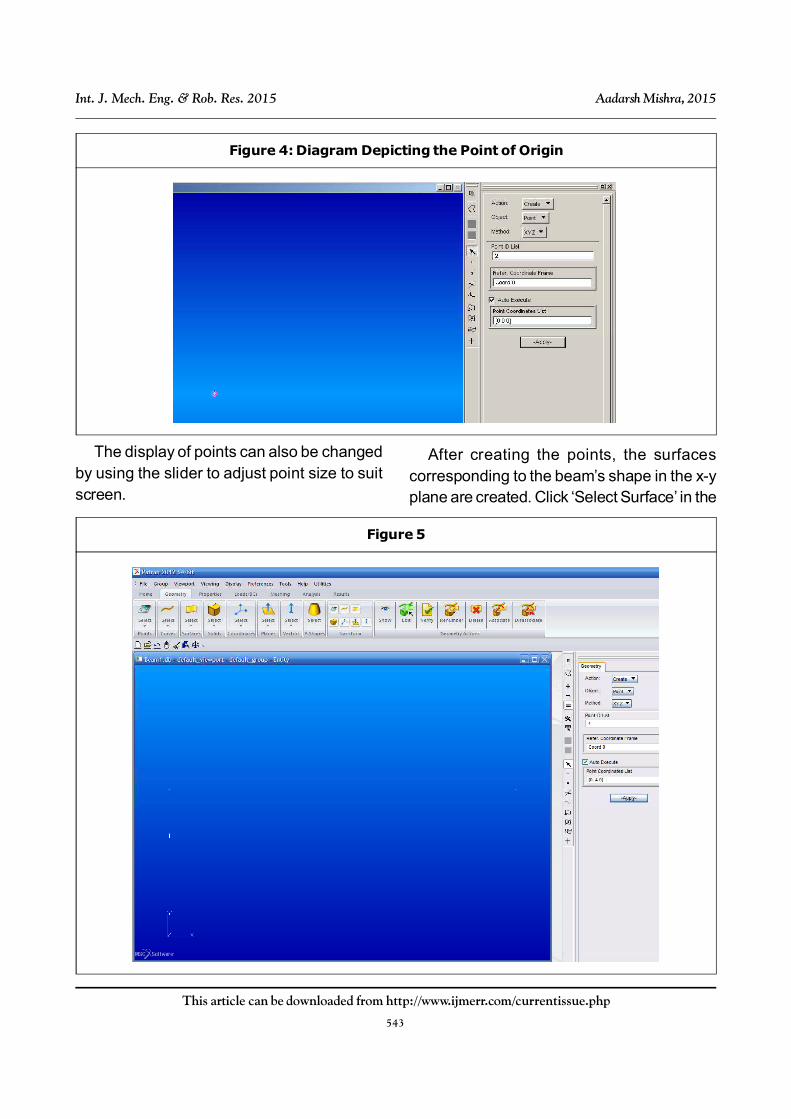
Figure 4: Diagram Depicting the Point of Origin

The display of points can also be changed

by using the slider to adjust point size to suit

screen.

After creating the points, the surfaces

corresponding to the beam’s shape in the x-y

plane are created. Click ‘Select Surface’ in the

Figure 5

544



Figure 6

Figure 7

545



Figure 8

Figure 9

546



Geometry Menu and Select ‘Vertex’ from the

options available. There will be a geometry

icon in which Create, Surface, Vertex will be

appearing. By placing the cursor in Vertex

boxes,select the corner points.

The surface is then divided into

Quadrilateral Finite Elements by selecting the

Meshing menu and then the surface mesher,

Options selected are Action: Create; Object:

Mesh; Type: Surface. The type of element

shape are selected as: Quadratic, IsoMesh

and Quad8. Finally, required length of element

is selected which will be the approximate

length of each element side.

Figure 10

Now putting the cursor in Surface List box,

select the surface by clicking on it, this will

change its colour. The name of surface

appears in the ‘Surface List’ box. The

analysis is then proceeded by clicking

‘Apply’.

The finite element mesh created is depicted

by the figure given below:

After the element meshing, specify the

required properties for the elements by

selecting the properties menu. In the properties

menu, there are options like: Isotropic

Materials and 2D properties.

547



Figure 11

Figure 12

548



Figure 13

Figure 14

Since the given Cantilever beam which is

being analysed is an Isotropic Material, Select

Isotropic Material from the menu. Select

Create, Isotropic, Manual Inputand then specify

the Material Name. Then click on the Input

properties.

A pop-up menu page opens in which the

properties of materials have to be specified.

The properties entered should be in S.I units.

However, any two of Elastic Modulus, Poisson

Ratio, and Shear Modulus are required. Click

‘Ok’ to return to Materials menu, and then Click

Apply to create the material.

Similarly, the properties of the Finite

Elements are also specified. Select the Shell

option within the 2D Properties.

549



� This option will select the Crate, 2D, Shell

menu.

� A shell element is a plane element that can

deflect in and perpendicular to its plane. It

is used to model a plate that has a thickness

that is considerably smaller than the

dimensions of the element.

� A shell element may also be curved (a

curved shell element) e.g., part of the wall

of a tube.

Further, there will be a Pop-up menu page

for specifying 2D Shell properties.

� Specify Property Set Name

� Click on the Materials Property Name icon

to list the materials available.

� Click on Input Properties

Now, a new popup Select Material menu

appears showing available materials. Click on

the required material. It will then be entered as

the Material Name entry and the popup will

disappear.

The shell element thickness has to be

specified in S.I Units. Finally, Click Ok.

The last step is to choose the Elements that

are to be allocated this property. Then click on

the ‘Select applicant region’.

� Put cursor in Select Members box

� Set surface pick option. The Pick options

available vary according to the choice to be

made.

� Select the surface on the drawing. Its outline

will change colour and its name will appear

in the Select Members box.

Figure 15

550



Figure 16

Figure 17

551



Figure 18

Figure 19

� Click Add which will transfer the selected

member to the Application Region.

� When the Application region is complete,

click ‘ok’.

RESULTS AND DISCUSSION

After applying the element properties in the

surface, specify the required Loads and

Restraints.

� Select Create, Force, Nodal.

� Specify Name for Load.

� Select the Input data.

� Click the Select Application region.

By default Geometry items are selected,

e.g., arcs, surfaces, points. This is called the

Geometry Filter.

552



� Put cursor in Select Nodes box of the new

window that appears.

� Select the ‘Node’ pick option. The Pick

options available vary according to the

choice to be made.

� Then click on the node to be loaded. The

selected load is indicated.

� Node number will then appear in the Select

Nodes box.

� Click Addto transfer Selected Nodes to the

Application Region.

� Click Ok to indicate that specifying the

Application Region is complete.

� The original window is then restored. Click

Apply to signify that the loading specified

is to be applied to the model

� When Apply is clicked the load applied is

illustrated on the model in magnitude and

direction.

Now specify required Restraints:

� Select Create, Displacement, Nodal

� Choose Name

� Click Input Data

Specify the translation restraint in the new

window: Fixed = No Translation.

Figure 20

553



Figure 21

� Insert the translation: < 0, 0, 0 >

This imposes a ball joint restraint at each

node selected.

� Insert the rotation: < 0,0,0>

� This prevents rotation about the x, y and z

axes at each node selected.

� These two restraints effectively fix any

nodes to which they are both applied.

� Click Okwhen complete.

As the cantilever beam is ‘built in’ at one

end, so the nodes at the end of the beam need

to be restrained. Hence cl ick ‘Select

Application region’.

554



Figure 22

� Select Geometry so that the edge of the

surface can be selected.

� Place cursor in Select Geometry Entities.

� Select the curve or edge pick option.

� Select the restrained edge with the cursor.

The selected curve will be shown in Select

Geometry Entities.When the correct edge is

chosen click Add to move the edge

specification to the Application Region, and

then click Ok.

The main Create, Displacement, Nodal

window will then appear.Click Apply to

implement the restraint.

A load of 20,000 N is made to act in the

negative y direction. Displacement boundary

condition is specified on curve for directions

1, 2, 3 and 4, 5, 6. This is applied to all finite

element nodes on the curve.

� Direction 1 is the x axis, 2 is y axis, and 3 is

z axis direction. These translation restraints

are indicated by single arrows.

555



Figure 23

Figure 24

556



Figure 25

Figure 26

557



Figure 27

Figure 28

558



Figure 29

Figure 30

559



Figure 31

� Direction 4 is rotation about the x axis, 2 is

rotation about the y axis, and 3 is rotation

about the z axis. These rotation restraints

are indicated by double arrows.

CONCLUSION

� To run the F.E. Analysis choose the Analysis

menu.

� Then select the Analyze Entire Model option.

� Select Analyze, Entire Model, Full Run.

� Click on Solution Type to make the Output

File selection for graphical results

presentation.

To run the analysis click on Apply which is

at the end of the menu list.A DOS window will

appear on the screen giving NASTRAN job

information.

Use the results menu to examine the

results:

� Quick Plot gives a simple tool to plot

deflected shape and fringe information.

� Results Plots for Deformation, Fringes,

Contours, Vector fields, Tensor fields are

sophisticated tools.

� Cursor gives values for particular results at

specified positions.

� Select Quick Plot.

� Select the results case. (There will be more

than one if the job has run more than once

or if it contains more than one loadcase).

� Select the kind of information to show using

coloured fringes, e.g., Displacements

Translational.

560



� Select the kind of information to show as a

deformation: Displacements Translational.

Constraint Forces is not a meaningful plot.

When a Fringe figure is selected as well as

a deflection the quantity plotted as a fringe is

shown as a contour plot superimposed on the

deflected shape. Here the displacement is

being plotted (u2 + v2 + w2), where (u, v, w) is

the displacement vector.

(u2 + v2 + w2) = 5.71 mm

The interface between two colours has the

stated contour value. Maximum and minimum

values are given on the plot.

� Maximum deflection is given as 0.0122. As

the data and properties have been specified

in SI units this result is in SI units, i.e., in

metres and is 0.0122 m or 12.2 mm.

� Beam theory result is a deflection of 12.05

mm on beam axis perpendicular to the axis.

The FEA result for this is 12.16 mm which

is a 0.9% difference.

In the diagram given below: X component of

the deflection is being plotted as a fringe.

ACKNOWLEDGMENT

I would like to dedicate this Research work to

my Father Late Ram Sewak Mishra and

Mother Kanak Lata Mishra.

REFERENCES

1. http://www.mscsoftware.com/product/

msc-nastran

2. Mishra A (2014a), “Anal ys is o f

Relation Between Friction and Wear”,

pp. 603-606.

3. Mishra A (2014b), “Microstructural

Analysis of Wear Debris”, pp. 416-421.

4. Mishra A (2014c), “The Generation of

Mechanically Mixed Layers (MMLS)

During Sliding Contact, pp. 578-582.

5. Mishra A (2014d), “Analysis of Application

of Oxide Surface as Environmental

Interface”, pp. 548-552.

6. Mishra A (2014e), “Effect of Hardness

on Sliding Behavior of Materials”,

pp. 566-569.

7. Mishra A (2014f), “Friction, Metallic

Transfer and Wear Debris of Sliding

Surface”, pp. 574-577.

8. Mishra A (2014g), “Influence of Oxidation

on the Wear of Alloys”, pp. 584-587.

9. Mishra A (2014h), “Analysis of Formation

of Oxide Surfaces”, pp. 553-556.

Date post:	14-May-2018
Category:	Documents
Upload:	trannhi
View:	215 times
Download:	2 times

Please note - Cardiff Universityorca.cf.ac.uk/70403/1/FEA.pdf · This is an Open Access document...

Documents