PM2.5 chemical composition and spatiotemporal variability ...€¦ · PM 2.5 chemical composition...

PM2.5 chemical composition and spatiotemporal variability during the

California Regional PM10/PM2.5 Air Quality Study (CRPAQS)

Judith C. Chow,1 L.-W. Antony Chen,1 John G. Watson,1 Douglas H. Lowenthal,1

Karen A. Magliano,2 Kasia Turkiewicz,2 and Donald E. Lehrman3

Received 1 July 2005; revised 7 December 2005; accepted 4 January 2006; published 25 May 2006.

[1] The 14-month-long (December 1999 to February 2001) Central California RegionalPM10/PM2.5 Air Quality Study (CRPAQS) consisted of acquiring speciated PM2.5

measurements at 38 sites representing urban, rural, and boundary environments in the SanJoaquin Valley air basin. The study’s goal was to understand the development ofwidespread pollution episodes by examining the spatial variability of PM2.5, ammoniumnitrate (NH4NO3), and carbonaceous material on annual, seasonal, and episodictimescales. It was found that PM2.5 and NH4NO3 concentrations decrease rapidly asaltitude increases, confirming that topography influences the ventilation and transport ofpollutants. High PM2.5 levels from November 2000 to January 2001 contributed to 50–75% of annual average concentrations. Contributions from organic matter differedsubstantially between urban and rural areas. Winter meteorology and intensive residentialwood combustion are likely key factors for the winter-nonwinter and urban-rural contraststhat were observed. Short-duration measurements during the intensive operating periodsconfirm the role of upper air currents on valley-wide transport of NH4NO3. Zones ofrepresentation for PM2.5 varied from 5 to 10 km for the urban Fresno and Bakersfield sites,and increased to 15–20 km for the boundary and rural sites. Secondary NH4NO3 occurredregion-wide during winter, spreading over a much wider geographical zone thancarbonaceous aerosol.

Citation: Chow, J. C., L.-W. A. Chen, J. G. Watson, D. H. Lowenthal, K. A. Magliano, K. Turkiewicz, and D. E. Lehrman (2006),

PM2.5 chemical composition and spatiotemporal variability during the California Regional PM10/PM2.5 Air Quality Study (CRPAQS),

J. Geophys. Res., 111, D10S04, doi:10.1029/2005JD006457.

1. Introduction

[2] The California Regional PM10/PM2.5 Air QualityStudy (CRPAQS) was undertaken with an overall goal ofunderstanding the causes of excessive PM (particulatematter) levels and to evaluate means to reduce them in centralCalifornia and its major geographical feature, the SanJoaquin Valley (SJV) [Watson et al., 1998]. The SJV repre-sents one of the largest PM2.5 and PM10 nonattainment areasin the United States (PM2.5 and PM10 are particles withaerodynamic diameters less than 2.5 and 10 micrometers[mm], respectively). It was expected that considerable vari-ability in emissions, meteorology, and terrain in the SJVwould translate into substantial differences in PM concen-tration and composition across the region. Knowledge ofthese spatiotemporal distributions of PM and its chemicalconstituents is essential for understanding source-receptorrelationships and chemical, physical, and meteorologicalprocesses that cause elevated PM levels in the SJV.

[3] The SJV air basin is bordered on the west by thecoastal mountain ranges and on the east by the SierraNevada range. These ranges converge at the TehachapiMountains at the southern end of the basin, �200 km southof Fresno (the largest population center within �150 kmalong a north-south line of the basin). Weather changesseasonally. Spring often brings weak, fast moving frontalpassages characterized by low moisture content and highwind speeds. Summer meteorology is driven by heating,which creates a thermal low-pressure system and a largeonshore pressure gradient between the coast and the desert.Fall and winter are influenced by the Great Basin High,with prolonged periods of air mass stagnation and limitedvertical mixing. Morning mixing depths are shallow andventilation rates are low during all seasons. Wind speeds arelow throughout the day during winter in the absence ofstorm systems. Relative humidity (RH) is highest in winterand lowest in summer and fall.[4] Central California emission source categories include

(1) small- to medium-sized point sources (e.g., powerstations, natural gas boilers, steam generators, incinerators,and cement plants); (2) area sources (e.g., resuspended dust,petroleum extraction operations, cooking, wildfires, andresidential wood combustion [RWC]); (3) mobile sources(e.g., cars, trucks, off-road heavy equipment, trains, andaircraft); (4) agricultural and ranching activities (e.g.,tilling, fertilizers, herbicides, and livestock); and (5) bio-

JOURNAL OF GEOPHYSICAL RESEARCH, VOL. 111, D10S04, doi:10.1029/2005JD006457, 2006

1Division of Atmospheric Sciences, Desert Research Institute, Reno,Nevada, USA.

2California Air Resources Board, Sacramento, California, USA.3Technical and Business Systems, Santa Rosa, California, USA.

Copyright 2006 by the American Geophysical Union.0148-0227/06/2005JD006457$09.00

D10S04 1 of 17

genic sources (e.g., nitrogen oxides [NOx] from biologicalactivity in soils and hydrocarbon emissions from plants).Agriculture is the main industry in the valley, where themajor crops are cotton, alfalfa, corn, safflower, grapes, andtomatoes. Cattle feedlots and dairies constitute most of theanimal husbandry in the region, along with chicken andturkey farms, which are major sources of ammonia (NH3)emissions.[5] Past studies [Chow et al., 1992, 1993a, 1996, 1998]

have shown that elevated PM concentrations frequentlyoccur in winter, when PM10 concentrations are primarilyin the PM2.5 size fraction. Chemical mass balance receptormodels [Magliano et al., 1999; Schauer and Cass, 2000]have attributed winter PM episodes in urban areas to RWCemissions, motor vehicle exhaust, and secondary ammoni-um nitrate (NH4NO3). NH4NO3 generally accounted for30–60% of PM2.5 during winter [Magliano et al., 1998a,1998b, 1999; Chow et al., 1999]. Vehicular exhaust andRWC emissions are mostly in the PM2.5 fraction withabundant organic carbon (OC) and elemental carbon (EC).[6] Watson and Chow [2002a] developed a conceptual

model that describes the interplay of emissions and mete-orology leading to transport of pollutants and formation ofwidespread PM2.5 episodes across the SJV in winter. Themodel begins with a shallow radiation surface inversion(100–200 m deep) which is decoupled from a valley-widemixed layer aloft between �1700 local time (LT) and�1100 LT the next morning. At night, the cities experiencea build up of primary pollutants emitted from traffic andRWC. Nitric acid (HNO3) can form in the upper layer duringnighttime hours through a series of reactions [Atkinson et al.,1986; Stockwell et al., 2000; Pun and Seigneur, 2001].Prevented from deposition by the surface inversion, thisHNO3 would be made available over rural areas with highNH3 emissions to rapidly create NH4NO3. Limited upperair observations [Lehrman et al., 1998] indicate thatwinds within the valley-wide layer often reach speedsof 1–6 m s�1 while surface winds are <1 m s�1. Thisimplies that secondary NH4NO3 can be mixed throughoutthe valley in one to two days. When radiative heatingbreaks the inversion after �1100 LT, turbulent mixingbetween the upper and surface layers intensifies, causinga net downward flux of NH4NO3, which escalates nearthe surface. In urban areas, this mixing also dilutes theconcentrations of primary pollutants, creating a complexdiurnal pattern of PM2.5 [Watson et al., 2002].[7] This paper (1) statistically summarizes CRPAQS

PM2.5 mass and chemical compositions, (2) investigateschemical closure for PM2.5 mass, (3) analyzes the spatio-temporal variability of PM2.5 and its chemical composition,(4) examines episodes of elevated PM2.5 during winter inthe context of the conceptual model of Watson and Chow[2002a], and (5) evaluates the zones of representation forPM2.5 sampling sites and their implications for future airquality monitoring and research.

2. Ambient Network

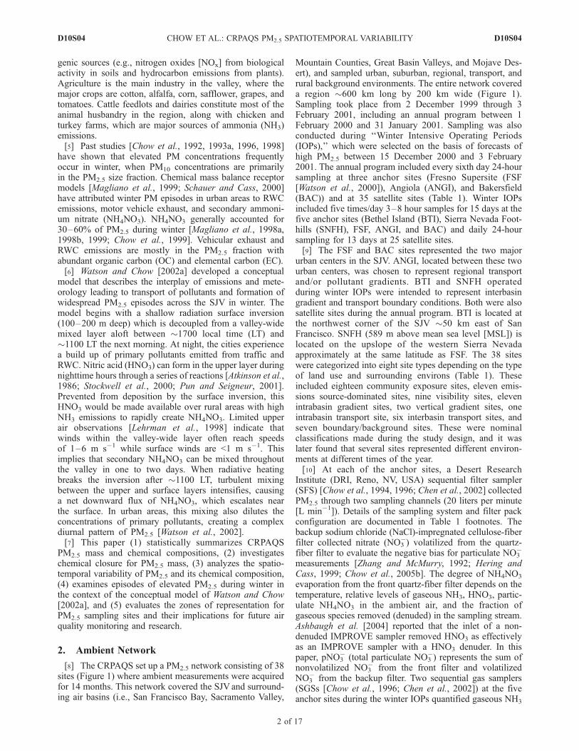
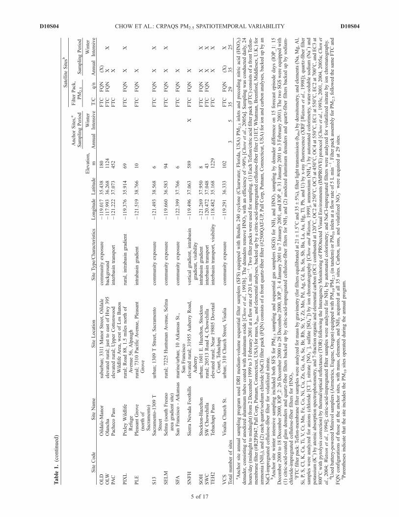
[8] The CRPAQS set up a PM2.5 network consisting of 38sites (Figure 1) where ambient measurements were acquiredfor 14 months. This network covered the SJV and surround-ing air basins (i.e., San Francisco Bay, Sacramento Valley,

Mountain Counties, Great Basin Valleys, and Mojave Des-ert), and sampled urban, suburban, regional, transport, andrural background environments. The entire network covereda region �600 km long by 200 km wide (Figure 1).Sampling took place from 2 December 1999 through 3February 2001, including an annual program between 1February 2000 and 31 January 2001. Sampling was alsoconducted during ‘‘Winter Intensive Operating Periods(IOPs),’’ which were selected on the basis of forecasts ofhigh PM2.5 between 15 December 2000 and 3 February2001. The annual program included every sixth day 24-hoursampling at three anchor sites (Fresno Supersite (FSF[Watson et al., 2000]), Angiola (ANGI), and Bakersfield(BAC)) and at 35 satellite sites (Table 1). Winter IOPsincluded five times/day 3–8 hour samples for 15 days at thefive anchor sites (Bethel Island (BTI), Sierra Nevada Foot-hills (SNFH), FSF, ANGI, and BAC) and daily 24-hoursampling for 13 days at 25 satellite sites.[9] The FSF and BAC sites represented the two major

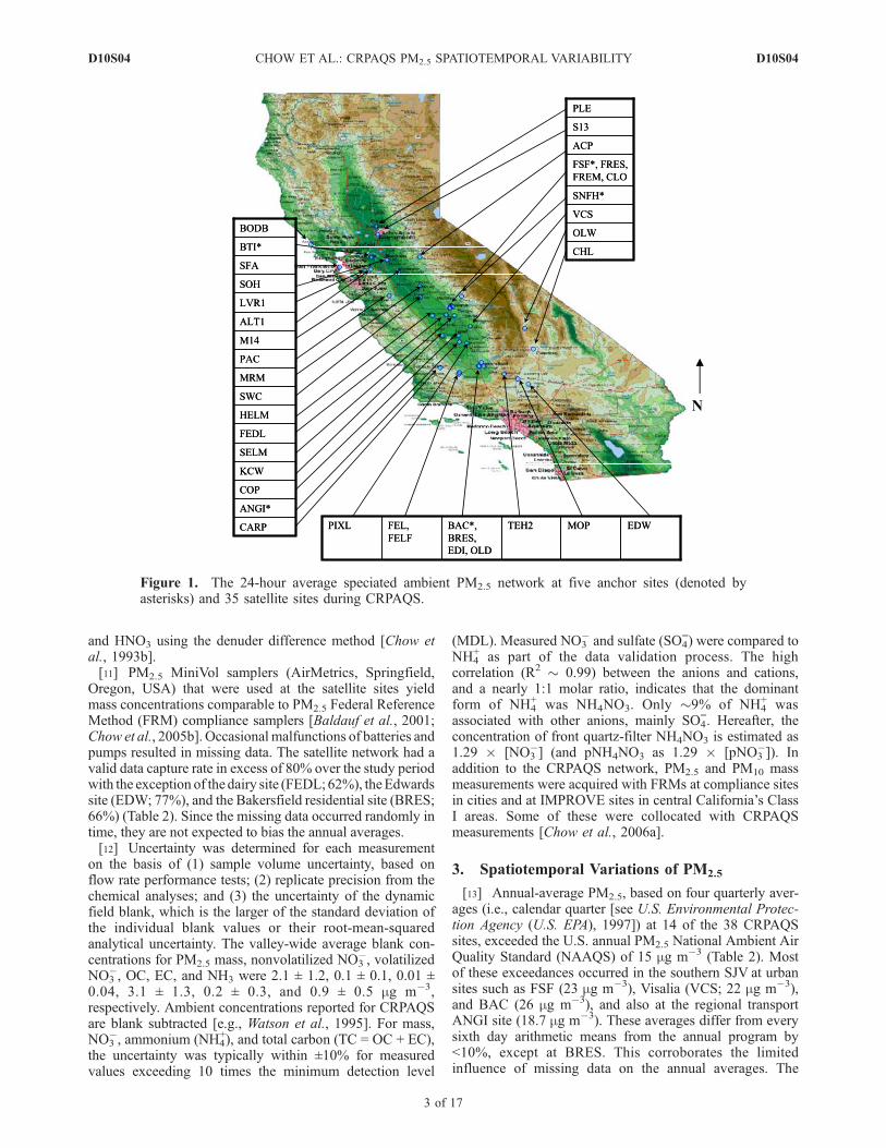
urban centers in the SJV. ANGI, located between these twourban centers, was chosen to represent regional transportand/or pollutant gradients. BTI and SNFH operatedduring winter IOPs were intended to represent interbasingradient and transport boundary conditions. Both were alsosatellite sites during the annual program. BTI is located atthe northwest corner of the SJV �50 km east of SanFrancisco. SNFH (589 m above mean sea level [MSL]) islocated on the upslope of the western Sierra Nevadaapproximately at the same latitude as FSF. The 38 siteswere categorized into eight site types depending on the typeof land use and surrounding environs (Table 1). Theseincluded eighteen community exposure sites, eleven emis-sions source-dominated sites, nine visibility sites, elevenintrabasin gradient sites, two vertical gradient sites, oneintrabasin transport site, six interbasin transport sites, andseven boundary/background sites. These were nominalclassifications made during the study design, and it waslater found that several sites represented different environ-ments at different times of the year.[10] At each of the anchor sites, a Desert Research

Institute (DRI, Reno, NV, USA) sequential filter sampler(SFS) [Chow et al., 1994, 1996; Chen et al., 2002] collectedPM2.5 through two sampling channels (20 liters per minute[L min�1]). Details of the sampling system and filter packconfiguration are documented in Table 1 footnotes. Thebackup sodium chloride (NaCl)-impregnated cellulose-fiberfilter collected nitrate (NO3

�) volatilized from the quartz-fiber filter to evaluate the negative bias for particulate NO3

�

measurements [Zhang and McMurry, 1992; Hering andCass, 1999; Chow et al., 2005b]. The degree of NH4NO3

evaporation from the front quartz-fiber filter depends on thetemperature, relative levels of gaseous NH3, HNO3, partic-ulate NH4NO3 in the ambient air, and the fraction ofgaseous species removed (denuded) in the sampling stream.Ashbaugh et al. [2004] reported that the inlet of a non-denuded IMPROVE sampler removed HNO3 as effectivelyas an IMPROVE sampler with a HNO3 denuder. In thispaper, pNO3

� (total particulate NO3�) represents the sum of

nonvolatilized NO3� from the front filter and volatilized

NO3� from the backup filter. Two sequential gas samplers

(SGSs [Chow et al., 1996; Chen et al., 2002]) at the fiveanchor sites during the winter IOPs quantified gaseous NH3

D10S04 CHOW ET AL.: CRPAQS PM2.5 SPATIOTEMPORAL VARIABILITY

2 of 17

D10S04

and HNO3 using the denuder difference method [Chow etal., 1993b].[11] PM2.5 MiniVol samplers (AirMetrics, Springfield,

Oregon, USA) that were used at the satellite sites yieldmass concentrations comparable to PM2.5 Federal ReferenceMethod (FRM) compliance samplers [Baldauf et al., 2001;Chow et al., 2005b]. Occasional malfunctions of batteries andpumps resulted in missing data. The satellite network had avalid data capture rate in excess of 80% over the study periodwith the exception of the dairy site (FEDL; 62%), theEdwardssite (EDW; 77%), and the Bakersfield residential site (BRES;66%) (Table 2). Since the missing data occurred randomly intime, they are not expected to bias the annual averages.[12] Uncertainty was determined for each measurement

on the basis of (1) sample volume uncertainty, based onflow rate performance tests; (2) replicate precision from thechemical analyses; and (3) the uncertainty of the dynamicfield blank, which is the larger of the standard deviation ofthe individual blank values or their root-mean-squaredanalytical uncertainty. The valley-wide average blank con-centrations for PM2.5 mass, nonvolatilized NO3

�, volatilizedNO3

�, OC, EC, and NH3 were 2.1 ± 1.2, 0.1 ± 0.1, 0.01 ±0.04, 3.1 ± 1.3, 0.2 ± 0.3, and 0.9 ± 0.5 mg m�3,respectively. Ambient concentrations reported for CRPAQSare blank subtracted [e.g., Watson et al., 1995]. For mass,NO3

�, ammonium (NH4+), and total carbon (TC = OC + EC),

the uncertainty was typically within ±10% for measuredvalues exceeding 10 times the minimum detection level

(MDL). Measured NO3� and sulfate (SO4

=) were compared toNH4

+ as part of the data validation process. The highcorrelation (R2 � 0.99) between the anions and cations,and a nearly 1:1 molar ratio, indicates that the dominantform of NH4

+ was NH4NO3. Only �9% of NH4+ was

associated with other anions, mainly SO4=. Hereafter, the

concentration of front quartz-filter NH4NO3 is estimated as1.29 � [NO3

�] (and pNH4NO3 as 1.29 � [pNO3�]). In

addition to the CRPAQS network, PM2.5 and PM10 massmeasurements were acquired with FRMs at compliance sitesin cities and at IMPROVE sites in central California’s ClassI areas. Some of these were collocated with CRPAQSmeasurements [Chow et al., 2006a].

3. Spatiotemporal Variations of PM2.5

[13] Annual-average PM2.5, based on four quarterly aver-ages (i.e., calendar quarter [see U.S. Environmental Protec-tion Agency (U.S. EPA), 1997]) at 14 of the 38 CRPAQSsites, exceeded the U.S. annual PM2.5 National Ambient AirQuality Standard (NAAQS) of 15 mg m�3 (Table 2). Mostof these exceedances occurred in the southern SJV at urbansites such as FSF (23 mg m�3), Visalia (VCS; 22 mg m�3),and BAC (26 mg m�3), and also at the regional transportANGI site (18.7 mg m�3). These averages differ from everysixth day arithmetic means from the annual program by<10%, except at BRES. This corroborates the limitedinfluence of missing data on the annual averages. The

Figure 1. The 24-hour average speciated ambient PM2.5 network at five anchor sites (denoted byasterisks) and 35 satellite sites during CRPAQS.


3 of 17

D10S04

Table

1.SummaryofCRPAQSAerosolMeasurementsat

theAnchorandSatellite

Sites

SiteCode

SiteNam

eSiteLocation

SiteType/Characteristics

Longitude

Latitude

Elevation,

m

AnchorSites,a

Sam

plingPeriod

Satellite

Sites

b

FilterPack,

PM

2.5

Sam

plingPeriod

Annual

Winter

Intensive

T/C

q/n

Annual

Winter

Intensive

ACP

AngelsCam

pelevated

rural;6850Studhorse

FlatRoad,Sonora

intrabasin

gradient

�120.491

38.006

373

FTCc

FQNd

XX

ALT1

Altam

ontPass

elevated

rural;FlynnRoad

exit,I-580

interbasin

transport

�121.660

37.718

350

FTC

XX

ANGI

Angiola-groundlevel

rural;360784th

Avenue,

Corcoran

intrabasin

gradient/transport,

verticalgradient,visibility

�119.538

35.948

60

XX

BAC

Bakersfield-5558

California

Street

urban;5558CA

Ave.

#430(STI)

#460(A

RB),Bakersfield

communityexposure,

visibility

�119.063

35.357

119

XX

BODG

BodegaMarineLab

marine;

BodegaMarineLab,2099

WestsideRoad,BodegaBay

boundary/background

�123.073

38.319

17

FTC

FQN

XX

BRES

BAC-residential

urban;7301Rem

ingtonAvenue,

Bakersfield

source:

woodburning

�119.084

35.358

117

FTC

FQN

XX

BTI

Bethel

Island

rural;5551Bethel

IslandRoad,

Bethel

Island

interbasin

transport

�121.642

38.006

2X

FTC

FQN

X

CARP

Carrizo

Plain

elevated

rural;SodaSpringsRoad,

0.5

milesouth

ofCalifornia

Valley

intrabasin

gradient,visibility

�119.996

35.314

598

FTC

X

CHL

ChinaLake

elevated

rural;Baker

site

visibility

�117.776

35.774

684

FTC

FQN

XCLO

Clovis

suburban;908N.Villa,Clovis

communityexposure

�119.716

36.819

108

FTC

FQN

XX

COP

Corcoran-Patterson

Avenue

rural;1520PattersonAve.,Corcoran

communityexposure

�119.566

36.102

63

FTC

FQN

(X)e

X

EDI

Edison

urban;4101Kim

ber

Avenue,

Bakersfield

intrabasin

gradient

�118.957

35.350

118

FTC

XX

EDW

EdwardsAirForce

Base

elevated

rural;northendof

Raw

insondeRoad,EdwardsAFB

intrabasin

gradient,visibility

�117.904

34.929

724

FTC

FQN

X

FEDL

feedlotordairy

rural;8555S.Valentine,

Fresno

(nearRaisinCity)

source:

cattle

�119.855

36.611

76

FTC

FQN

XX

FEL

Fellows

elevated

rural;across

from

25883Hwy33,

Fellows

source:

oilfields

�119.546

35.203

359

FTC

FQN

XX

FELF

foothillsabove

Fellows

elevated

rural;TexacoPump

Site47-1,Fellows

intrabasin

gradient

�119.557

35.171

512

FTC

FQN

XX

FREM

FresnoMV

urban;Pole

#16629,2253E.Shields

Ave.,Fresno

source:

motorvehicle

�119.783

36.780

96

FTC

FQN

XX

FRES

residential

area

near

FSF,withwood

burning

urban;Pole

#16962,3534Virginia

Lane,

Fresno

source:

woodburning

�119.768

36.783

97

FTC

FQN

(X)

X

FSF

Fresno-3425FirstStreet

urban;3425FirstStreet,Fresno

communityexposure,

visibility

�119.773

36.782

97

XX

HELM

agricultural

fields/Helm-central

FresnoCounty

rural;nearPlacerandSpringfield

intrabasin

gradient

�120.177

36.591

55

FTC

FQN

XX

KCW

Kettlem

anCity

rural;OmahaAvenue2miles

westof

Hwy41,Kettlem

anCity

intrabasin

gradient

�119.948

36.095

69

FTC

XX

LVR1

Livermore

-new

site

rural;793RinconStreet,Livermore

interbasin

transport

�121.784

37.688

138

FTC

FQN

XX

M14

Modesto

14th

St.

urban;81414th

Street,Modesto

communityexposure

�120.994

37.642

28

FTC

FQN

(X)

XMOP

Mojave-Poole

elevated

rural;923Poole

Street,

Mojave

communityexposure

�118.148

35.051

832

FTC

FQN

X

MRM

Merced-m

idtown

suburban;2334M

Street,Merced

communityexposure

�120.481

37.308

53

FTC

FQN

XX


4 of 17

D10S04

Table

1.(continued)

SiteCode

SiteNam

eSiteLocation

SiteType/Characteristics

Longitude

Latitude

Elevation,

m

AnchorSites,a

Sam

plingPeriod

Satellite

Sites

b

FilterPack,

PM

2.5

Sam

plingPeriod

Annual

Winter

Intensive

T/C

q/n

Annual

Winter

Intensive

OLD

Oildale-Manor

suburban;3311

ManorStreet,Oildale

communityexposure

�119.017

35.438

180

FTC

FQN

(X)

OLW

Olancha

elevated

rural;justto

eastofHwy395

background

�117.993

36.268

1124

FTC

FQN

XX

PAC

PachecoPass

elevated

rural;Upper

Cottonwood

Wildlife

Area,

westofLosBanos

interbasin

transport

�121.222

37.073

452

FTC

X

PIX

LPixleyWildlife

Refuge

rural;Road

88,1.5

miles

northof

Avenue56,Alpaugh

rural,intrabasin

gradient

�119.376

35.914

69

FTC

FQN

XX

PLE

PleasantGrove

(northof

Sacramento)

rural;7310Pacific

Avenue,

Pleasant

Grove

intrabasin

gradient

�121.519

38.766

10

FTC

FQN

X

S13

Sacramento-1309T

Street

urban;1309TStreet,Sacramento

communityexposure

�121.493

38.568

6FTC

FQN

XX

SELM

Selma(south

Fresno

area

gradientsite)

rural;7225Huntsman

Avenue,

Selma

communityexposure

�119.660

36.583

94

FTC

FQN

XX

SFA

San

Francisco-Arkansas

marine/urban;10ArkansasSt.,

San

Francisco

communityexposure

�122.399

37.766

6FTC

FQN

X

SNFH

SierraNevadaFoothills

elevated

rural;31955Auberry

Road,

Auberry

verticalgradient,intrabasin

gradient,visibility

�119.496

37.063

589

XFTC

FQN

X

SOH

Stockton-H

azelton

urban;1601E.Hazelton,Stockton

intrabasin

gradient

�121.269

37.950

8FTC

FQN

XX

SWC

SW

Chowchilla

rural;20513Road

4,Chowchilla

interbasin

transport

�120.472

37.048

43

FTC

FQN

XX

TEH2

TehachapiPass

elevated

rural;Near19805Dovetail

Court,Tehachapi

interbasin

transport,visibility

�118.482

35.168

1229

FTC

XX

VCS

Visalia

ChurchSt.

urban;310ChurchStreet,Visalia

communityexposure

�119.291

36.333

102

FTC

FQN

(X)

XTotalnumber

ofsites

35

35

29

35

25

aAnchorsite

annual

samplingprogram

usedDRImedium-volumesequential

filter

samplers

(SFS)equipped

withBendix

240cyclone(Clearwater,Florida,

USA)PM

2.5inlets

andprecedingnitricacid

(HNO3)

denuder,consistingofanodized

aluminum

tubes

coated

withaluminum

oxide[Chowetal.,1993b].ThedenudersremoveHNO3withan

efficiency

of>90%

[Chowet

al.,2005a].Sam

plingwas

conducted

daily,24

hours/day

(midnightto

midnight)from

2Decem

ber1999to

3February2001ataflowrateof20Lmin

�1.Twofilterpackswereusedforsampling.(1)EachTeflon/citricacid

filterpack(FTC)consistsofafrontTeflon-

mem

branefilter(#R2PJ047,PallCorp,Putnam

,Connecticut,USA)formass,babs,andelem

entalanalyses,backed

upbyacitric-acid-impregnated

cellulose-fiberfilter(31ET,Whatman,Brentford,Middlesex,U.K.)for

ammonia(N

H3),and(2)each

quartz/sodium

chloride(N

aCl)filter

pack(FQN)consistsofafrontquartz-fiber

filter

(#2500QAT-U

P,PallCorp,Putnam

,Connecticut,USA)forionandcarbonanalyses,backed

upbyan

NaC

l-im

pregnated

cellulose-fiber

filter

forvolatilizednitrate.

bAnchorsite

winterintensivesamplingincluded

both

SFSforPM

2.5samplingandsequential

gas

samplers

(SGS)forNH3andHNO3samplingbydenuder

difference

on15forecast

episodedays(IOP_1:15

Decem

ber

2000to

18Decem

ber

2000,IO

P_2:26Decem

ber

2000to

28Decem

ber

2000,IO

P_3:4January2001to

7January2001,andIO

P_4:31January2001to

3February2001).ThetwoSGSwereequipped

with

(1)citric-acid-coated

glass

denudersandquartz-fiber

filtersbacked

upbycitric-acid-impregnated

cellulose-fiber

filtersforNH3and(2)anodized

aluminum

denudersandquartz-fiber

filtersbacked

upbysodium-

chloride-im

pregnated

cellulose-fiber

filtersforHNO3.

cFTCfilter

pack:Teflon-m

embranefilter

sampleswereanalyzedformassbygravim

etry

(forfiltersequilibratedat21±1.5�C

and35±5%),filter

lighttransm

ission(b

abs)bydensitometry,andelem

ents(N

a,Mg,Al,

Si,P,S,Cl,K,Ca,Ti,V,Cr,Mn,Fe,Co,Ni,Cu,Zn,Ga,As,Se,Br,Rb,Sr,Y,Zr,Mo,Pd,Ag,Cd,In,Sn,Sb,Ba,La,Au,Hg,Tl,Pb,andU)byx-ray

fluorescence

(XRF[W

atsonet

al.,1998]);quartz-fiber

filter

sampleswereanalyzedforanions(chloride[Cl�],nitrate

[NO3�],sulfate[SO4=])byionchromatography[ChowandWatson,1999],am

monium

(NH4+)byautomated

colorimetry,water-soluble

sodium

(Na+)and

potassium

(K+)byatomicabsorptionspectrophotometry,and7-fractionorganicandelem

entalcarbon(O

C1combusted

at120�C

,OC2at250�C

,OC3at450�C

,OC4at550�C

,EC1at550�C

,EC2at700�C

,andEC3at

800�C

withpyrolysiscorrection)bythermal/opticalreflectance

(TOR)followingtheInteragency

MonitoringofPROtected

VisualEnvironments(IMPROVE)protocol[Chowetal.,1993c,2001,2004,2005a;Chen

etal.,2004;Watsonet

al.,1994];citric-acid-impregnated

filter

sampleswereanalyzedforNH3byautomated

colorimetry;andNaC

l-im

pregnated

filterswereanalyzedforvolatilizednitrate

byionchromatography.

dUsedbattery-powered

Minivolsamplers(A

irmetrics,Eugene,Oregon)equipped

withPM

10/PM

2.5(intandem

)orPM

10inletsataflowrateof5Lmin

�1.Filterpackassembly

forPM

2.5followed

thesameFTCand

FQN

configurationsofthose

attheanchorsites,withmass,elem

ents,andNH3acquired

atall35sites.Carbon,ions,andvolatilizedNO3�wereacquired

at29sites.

eParentheses

indicatethat

thesite

includes

thePM

10sitesoperated

duringtheannual

program.


5 of 17

D10S04

Table

2.SummaryofPM

2.5MassandChem

ical

Compositionat

38Sites

DuringCRPAQSa

Site

Code

14-M

onth

b/

Annualc

Valid

PM

2.5

Measurements

SpringMean

PM

2.5,dmg

m�3

Summer

Mean

PM

2.5,dmg

m�3

FallMean

PM

2.5,dmg

m�3

WinterMean

PM

2.5,dmg

m�3

Annual

MeansFrom

Quarters,e

mgm

�3

Annual

Mean

PM

2.5,cmg

m�3

14-M

onth

MeanPM

2.5,b

mgm

�3

Maxim

um

PM

2.5,mg

m�3

Maxim

um

Date

Chigh,f

mgm

�3

Clow,g

mgm

�3

Fhigh,h

%

Annual

NH4NO3

(Front),i

mgm

�3

Annual

NH4NO3

(Backup),j

mgm

�3

Annual

OM,k

mgm

�3

Annual

EC,

mgm

�3

Annual

(NH4) 2SO4,l

mgm

�3

Annual

Crustal,m

mgm

�3

Reconstructed

PM

2.5Mass,n

mgm

�3

PM

2.5Mass

Closure,o%

ACP

72/61

3.9

±2.1

3.6

±1.6

3.6

±2.2

5.0

±5.4

3.4

3.4

±2.1

4.2

±3.6

18.9

1/7/2000

3.5

3.4

25.5

1.0

0.1

3.8

0.9

1.1

0.4

7.6

223

ALT1

68/61

4.2

±1.8

5.1

±2.6

6.1

±10.2

13.3

±18.7

7.2

7.3

±11.7

7.8

±12.2

71.7

1/7/2001

16.8

3.9

58.6

��

��

��

��

��

0.3

��

��

ANGI

55/50

10.9

±3.9

11.4

±5.6

20.6

±26.7

29.1

±31.0

18.7

19.1

±23.7

19.3

±23.1

123.4

1/7/2001

41.4

11.3

55.0

8.1

1.5

5.3

0.8

2.0

3.0

19.6

103

BAC

66/57

19.8

±12.8

13.3

±2.9

23.2

±22.0

43.5

±36.7

26.0

27.0

±27.5

28.1

±27.7

132.7

1/1/2001

56.9

15.3

55.4

9.8

2.4

9.9

2.0

2.6

3.4

28.3

105

BODG

67/57

10.5

±4.9

4.6

±4.1

5.5

±4.3

14.8

±9.8

8.9

9.3

±7.8

10.0

±8.1

35.3

1/19/2001

13.6

7.9

36.3

1.6

0.1

1.6

0.4

1.9

0.2

10.2

110

BRES

45/40

7.9

±3.1

7.6

±2.5

20.1

±27.6

53.6

±42.1

43.7

27.9

±36.5

30.6

±36.7

158.9

1/1/2001

59.1

7.1

73.5

10.4

1.0

10.0

2.8

2.1

1.4

27.4

98

BTI

72/61

4.1

±1.9

4.5

±2.9

7.0

±11.8

18.5

±19.2

8.8

8.9

±13.9

10.0

±14.2

76.6

1/7/2001

22.8

3.9

65.8

3.5

0.1

4.1

1.3

1.7

0.7

12.2

137

CARP

63/63

4.2

±2.3

3.4

±2.2

7.5

±8.1

8.3

±10.0

5.5

6.0

±7.0

6.2

±7.4

32.6

1/19/2001

11.8

3.9

50.4

��

��

��

��

��

0.9

��

��

CHL

60/51

2.1

±1.3

3.3

±2.5

1.4

±1.4

5.6

±16.4

1.7

1.9

±1.8

3.4

±9.8

74.5

1/7/2000

0.8

2.4

9.9

0.4

0.2

4.1

0.8

1.0

0.4

7.1

375

CLO

66/56

7.8

±3.4

8.6

±2.5

21.4

±31.0

47.0

±38.2

20.6

20.8

±27.8

25.3

±32.0

130.1

1/1/2001

55.6

9.1

67.0

7.8

0.8

9.6

2.5

1.9

1.2

23.5

113

COP

71/60

10.0

±7.0

8.0

±1.7

20.0

±19.2

37.8

±35.7

17.9

18.2

±22.6

21.9

±26.5

124.7

1/7/2001

42.3

9.4

59.9

8.7

0.7

7.2

1.7

2.0

1.6

21.8

120

EDI

64/55

10.0

±5.7

10.5

±3.3

32.2

±43.8

38.3

±40.0

24.9

24.5

±34.5

24.9

±33.2

160.8

1/1/2001

48.0

14.8

51.9

��

��

��

��

��

3.1

��

��

EDW

50/47

4.5

±2.1

6.3

±1.3

5.0

±4.7

5.1

±4.9

5.0

5.3

±3.6

5.3

±3.7

16.9

9/21/2000

5.6

5.3

26.1

1.2

0.7

4.0

0.8

1.5

0.8

8.8

165

FEDL

38/38

��

27.8

±12.3

25.3

±15.3

38.6

±32.7

28.8

29.9

±21.3

29.9

±21.3

115.7

1/7/2001

38.4

23.7

35.0

10.6

0.2

9.7

1.9

2.3

3.4

29.0

97

FEL

71/61

7.5

±6.9

5.4

±1.5

13.4

±19.2

20.1

±20.6

12.2

12.2

±16.4

12.7

±16.4

74.2

1/1/2001

30.0

5.9

63.0

5.4

0.8

5.5

1.1

2.1

1.2

15.9

131

FELF

70/60

5.1

±2.8

4.9

±1.7

13.2

±18.1

19.6

±18.3

11.6

11.6

±15.4

12.0

±15.1

69.4

1/1/2001

29.5

5.1

65.8

6.5

0.7

5.2

0.9

2.2

0.6

15.9

137

FREM

67/60

9.7

±3.6

9.1

±2.9

21.8

±27.2

56.5

±47.7

24.8

25.3

±35.2

27.6

±36.3

176.0

1/1/2001

67.6

9.9

69.5

8.1

0.8

13.9

3.7

2.0

1.2

29.7

118

FRES

66/57

9.0

±3.9

7.8

±2.7

21.2

±27.0

55.9

±46.5

22.8

24.2

±33.9

28.2

±37.0

169.4

1/1/2001

63.3

8.9

70.3

7.6

0.8

11.7

2.9

1.9

0.8

25.7

106

FSF

71/60

11.2

±6.0

9.4

±2.9

20.1

±21.9

53.9

±41.5

23.3

23.7

±29.4

28.4

±33.4

148.3

1/1/2001

60.0

10.6

65.4

5.2

2.6

10.4

2.0

1.8

1.5

21.5

90

HELM

70/59

5.0

±2.0

5.5

±2.1

12.7

±15.5

25.9

±28.5

11.8

11.8

±16.3

14.4

±20.7

114.8

12/26/1999

30.8

5.3

66.1

6.5

0.7

5.0

1.4

1.8

0.8

16.2

138

KCW

64/55

6.1

±3.3

6.1

±2.2

13.9

±26.7

32.6

±32.7

10.9

12.9

±19.3

16.8

±25.3

112.7

1/7/2000

29.9

5.9

62.9

��

��

��

��

��

0.9

��

��

LVR1

72/61

6.2

±4.1

6.0

±3.6

8.7

±11.1

20.6

±22.3

10.5

10.6

±14.9

11.9

±15.8

95.4

1/7/2001

24.7

5.6

59.6

3.3

0.2

6.2

2.4

1.6

0.3

14.6

137

M14

71/60

6.1

±2.2

7.1

±5.1

16.0

±22.7

41.9

±34.4

17.3

17.3

±25.5

21.0

±27.7

136.1

1/7/2001

47.8

6.2

72.1

6.2

0.6

9.2

2.4

2.0

0.6

21.1

122

MOP

69/58

5.6

±3.6

5.3

±1.9

4.8

±3.8

2.8

±3.3

4.4

4.3

±3.3

4.4

±3.4

15.6

11/14/2000

2.9

4.8

16.6

1.0

0.5

5.0

1.1

1.4

0.6

9.5

219

MRM

72/61

7.0

±3.5

6.8

±3.3

13.0

±13.2

36.6

±28.3

13.9

14.0

±14.4

18.9

±22.5

115.9

12/20/1999

32.4

7.4

59.3

6.5

0.4

8.9

2.2

1.8

0.7

20.7

148

OLD

65/55

9.5

±5.7

7.6

±2.0

23.1

±26.8

40.9

±38.4

21.5

21.1

±29.0

23.5

±29.9

140.6

1/1/2001

52.6

8.2

68.3

11.0

1.0

9.0

1.9

2.6

1.3

26.3

125

OLW

65/54

3.1

±4.4

5.5

±9.9

1.5

±1.3

3.0

±3.9

3.2

3.1

±5.8

3.2

±5.6

39.2

7/29/2000

1.9

3.6

15.3

0.3

0.1

4.0

0.7

0.8

0.7

7.0

224

PAC

71/61

3.5

±2.1

2.9

±1.6

4.6

±8.3

14.2

±17.6

6.1

6.1

±9.2

7.4

±12.1

64.3

12/26/1999

15.0

2.9

62.9

��

��

��

��

��

0.1

��

��

PIX

L69/61

9.8

±6.7

10.0

±8.2

17.7

±14.5

38.6

±33.0

18.4

18.5

±21.5

21.2

±24.1

106.6

1/7/2001

42.9

9.8

59.4

9.9

0.4

6.0

1.6

2.2

1.3

21.6

117

PLE

70/59

6.4

±2.5

6.4

±2.5

9.1

±9.8

18.0

±18.0

9.1

9.1

±9.1

11.1

±12.7

66.3

12/20/1999

18.6

5.6

52.4

3.0

0.2

6.8

1.9

1.4

0.5

14.2

155

S13

68/58

4.5

±1.6

4.9

±2.8

10.3

±10.8

24.4

±24.0

10.9

11.1

±14.8

13.2

±17.7

90.2

12/20/1999

27.8

4.7

66.2

3.8

0.2

7.2

2.3

1.5

0.7

16.3

147

SELM

71/61

11.4

±7.3

8.9

±3.3

18.0

±16.5

41.2

±34.7

18.2

18.3

±19.4

22.8

±26.0

110.4

12/26/1999

40.3

10.5

56.1

8.3

0.8

7.8

2.3

2.2

1.1

22.5

122

SFA

72/61

8.0

±4.7

5.1

±3.7

9.0

±7.9

16.2

±14.7

9.2

9.2

±8.6

10.5

±10.8

63.4

12/26/1999

18.3

6.0

50.5

3.1

0.1

4.5

1.8

2.0

0.5

13.8

150

SNFH

70/60

6.3

±3.7

5.6

±1.8

8.0

±4.4

18.1

±18.6

8.5

8.5

±8.1

10.7

±12.6

70.2

1/1/2000

15.6

5.9

46.8

2.8

0.4

6.4

1.3

1.6

0.6

13.4

157

SOH

70/59

5.4

±2.3

7.2

±5.2

9.4

±9.0

31.1

±27.3

12.7

12.8

±16.5

16.1

±20.7

103.3

12/20/1999

32.8

6.0

64.7

4.8

0.6

7.2

2.2

1.9

0.6

17.9

140

SWC

70/59

7.4

±2.5

6.5

±2.2

13.7

±15.5

28.0

±28.7

13.1

12.9

±15.7

16.0

±20.9

97.4

12/26/1999

32.5

6.8

61.5

6.3

0.7

4.5

1.4

1.6

0.8

15.6

122

TEH2

64/53

9.1

±3.7

6.5

±2.7

7.4

±5.1

5.6

±8.9

7.3

7.3

±6.2

6.8±6.2

35.4

12/8/2000

7.3

7.3

25.1

��

��

��

��

��

0.5

��

��

VCS

72/61

14.1

±8.7

9.5

±3.3

18.6

±18.1

46.9

±37.2

21.7

21.9

±24.7

25.9

±28.8

123.7

1/1/2001

50.3

11.8

58.7

9.5

0.8

9.8

2.4

2.3

1.3

26.5

121

aAnchorsitesarecoded

inbold;referto

Table

1forsite

codes.

bConsistsof72every-6th-day

samplingfrom

2Decem

ber

1999to

3February2001.

cConsistsof61every-6th-day

samplingfrom

1February2000to

31January2001(CRPA

QSannual

period).

dSeasonal

averages

ofspring(M

arch

toMay),summer

(Juneto

August),fall(September

toNovem

ber),andwinter(D

ecem

ber

toFebruary)fortheCRPAQSannual

period.

eArithmeticmeansofthefourcalendar

quarters:Januaryto

March,Aprilto

June,July

toSeptember,andOctober

toDecem

ber

duringtheCRPA

QSannualperiod.Januaryisfrom

2001andtherestofthemonthsare

from

2000.Italicsindicate<75%

coveragein

atleastonequarter.

f AverageofhighPM

2.5period(1

Novem

ber

2000to

31January2001).

gAverageoflow

PM

2.5period(1

February2000to

31October

2000).


6 of 17

D10S04

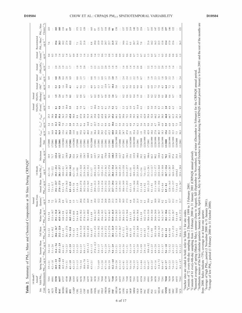
annual average determined by sixth day sampling is used insubsequent analyses rather than the annual average of quar-terly averages required to determine NAAQS attainment.[14] The PM2.5 concentration decreased rapidly toward

the higher-elevation valley boundary (Figure 2a). Three

sites in Bakersfield (residential BRES site, urban BAC site,and interbasin gradient Edison [EDI] site, all �118 m aboveMSL) reported consistently high annual-average PM2.5

concentrations of 24–28 mg m�3, despite the fact that eachsite represents different microenvironments. Tehachapi

Notes to Table 2.hFhigh = [Chigh/(Chigh + 3 � Clow)] � 100.i1.29 � ([NO3

�]FRONT).j1.29 � ([NO3

�]BACKUP).k1.4 � [OC].l1.38 � [SO4

2�].m2.2 � [Al] + 2.49 � [Si] + 1.63 � [Ca] + 2.42 � [Fe] + 1.94 � [Ti].nNH4NO3 (front filter, nonvolatilized NH4NO3) + OM +EC + (NH4)2SO4 + crustal material (CM) + trace elements (other than geological material) and

sea salt (Na+ + Cl�).o(Summed PM2.5 mass/annual mean PM2.5) � 100%.

Figure 2. Spatial distribution of (a) annual PM2.5 concentration (1 February 2000 to 31 January 2001)during CRPAQS and geographical cross sections A, B, and C and (b) the sampling sites and cross sectionD. Contours are determined with a two-dimensional cubic-spline algorithm using only sites with >70%valid measurements. The stars indicate locations of the sampling sites.


7 of 17

D10S04

(TEH2), an interbasin transport site, located �50 km to thesoutheast of EDI at 1229 m above MSL, recorded anannual-average PM2.5 concentration of 7.3 mg m�3. Theannual-average PM2.5 concentration decreased further at theMojave Desert (EDW; 724 m above MSL) and Mojave-Pool (MOP; 832 m above MSL) sites, averaging only 4.3–5.4 mg m�3. Similarly, annual-average PM2.5 concentrationdecreased from 24 mg m�3 at FSF, to 21 mg m�3 at Clovis(CLO; 108 m above MSL, a suburban site �10 km east ofFSF), and to 8.5 mg m�3 at SNFH (589 m above MSL,33 km east of CLO). This reflects the influence oftopography and the generally low vertical mixing potentialdue to weak boundary layer turbulence on many of the highPM2.5 days. North of Fresno, the annual-average PM2.5

concentration was relatively low even at the urban centersof Sacramento (S13, 11.1 mg m�3) and San Francisco (SFA,9.2 mg m�3), with the highest annual-average concentrationof 17.3 mg m�3 observed at Modesto (M14).[15] The stable atmosphere surrounding the Sierra

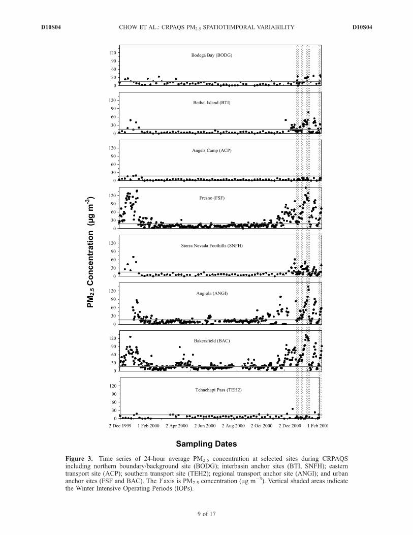
Nevada and coastal mountains prevents precursor gasesand PM released in the SJV from rapidly dispersing. Tosome extent, the valley is also isolated from the influencesof outside sources. This is especially true for the southernSJV because the elevation of the valley floor generallyincreases from north to south as far as Fresno anddescends south of Fresno. The five most northwesternsites in this network, located at Bodega Bay (BODG),BTI, SFA, S13, and Stockton (SOH), all have elevationsless than 10 m above MSL. Marine air enters the SJVthrough the Carquinez Straight east of the San FranciscoBay area, leading to the lower PM2.5 in the northernvalley. The highest annual-average water-soluble sodium(Na+; a sea salt marker) concentrations were found atcoastal sites west of the valley (BODG, SFA, and Liver-more (LVR1)) where annual-average PM2.5 and Na+ con-centrations were 9.3 and 1.7, 9.2 and 0.58, and 10.6 and0.32 mg m�3, respectively. Three sites in the northernvalley, S13, BTI, and SOH, also experienced higherannual-average Na+ concentration (0.24–0.28 mg m�3)than FSF (0.11 mg m�3) and BAC (0.13 mg m�3). Thelower PM2.5 concentrations at S13 and SOH comparedwith higher concentrations at down-valley urban sitesdemonstrate the influence of clean marine air in thenorthern valley.[16] As shown in Figure 3, 24-hour PM2.5 concentrations

at FSF were low from mid-February 2000 to late October2000, but frequently exceeded 15 mg m�3 from Novemberto January, and reached a maximum of 148 mg m�3 on 1January 2001. A similar temporal pattern was found atBAC, which often reported higher PM2.5 concentrationsthan FSF. In addition to the increased RWC emissionsduring winter [Magliano et al., 1999; Schauer and Cass,2000], the meteorological effect (i.e., prolonged Great Basinhighs causing subsidence) on the ventilation of pollutantsand formation of secondary aerosol also contributes to theseasonal cycle. The regional transport ANGI site, located inthe ancient Tulare Lake bed, surrounded by farm fields andsparse residences, experienced wintertime PM2.5 concentra-tions similar to those at FSF and BAC. High winterconcentrations at the other two interbasin anchor sites(BTI and SNFH) were much less pronounced. BODG inFigure 3 represents the northern boundary/background site

of the SJV, while the ACP (373 m above MSL) and TEH2(1229 m above MSL) sites represent the eastern andsouthern intra and interbasin transport sites. No appreciableseasonal variations were observed at these boundary andtransport sites, especially at BODG and TEH2; the back-ground PM2.5 level, which is often influenced by long-range(synoptic-scale) transport, appeared to be consistent year-round.[17] The patterns of temporal variations in Figure 3 are

consistent with limited differences in PM2.5 spring (Marchto May) and summer (June to August) averages (Table 2).Urban-rural contrast in the northern SJV was minimalduring spring and summer. For example, average springPM2.5 concentration at BODG (10.5 mg m�3) comparedwell with those at FSF (11.2 mg m�3) and the Fresnoresidential site (FRES; 9.0 mg m�3). However, the source-dominated dairy site (FEDL) reported elevated averagePM2.5 concentrations (25–28 mg m�3) during summer andfall, and reached a maximum of 39 mg m�3 in winter.[18] CRPAQS annual measurements may be divided into

high (Chigh; 1 November 2000 to 31 January 2001) andlow (Clow; 1 February 2000 to 31 October 2000) PM2.5

periods. As shown in Table 2, PM2.5 approached 15 mg m�3

at Bakersfield (BAC, EDI), even during the low period.The maximum Clow occurred at the source-dominatedFEDL site (24 mg m�3). The contributions of PM2.5 duringChigh to annual averages (i.e., Fhigh, defined in Table 2),ranged from 13% at China Lake (CHL) to 72% at M14.Chigh contributed more than 50% of annual-average PM2.5

concentrations at most sites inside the valley, 55% at theBAC, and 63% at the FSF urban centers. Fhigh was <25%only at three sites in the network: CHL (10%), MOP(17%), and Olancha (OLW; 15%), all of which are locatedin the Mojave Desert or Great Basin Valleys. The slightlyhigher Clow than Chigh at these desert sites is consistentwith previously observed transport from the SJV andsouthern California during nonwinter months [Green etal., 1992].

4. PM2.5 Chemical Composition

[19] Table 2 presents the annual-average concentrationsof five main PM2.5 components (i.e., NH4NO3, ammoniumsulfate [(NH4)2SO4], organic matter [OM = 1.4 � OC], EC,and crustal material), as well as the PM2.5 mass balance.CRPAQS confirms previous studies conducted in the SJV[e.g., Chow et al., 1992, 1993a, 1996, 1999] that PM2.5

consists mainly of NH4NO3 and carbonaceous material.Volatilized NH4NO3 from the backup filter is not includedin the reconstructed mass (defined in Table 2) since PM2.5

mass determined from Teflon-membrane filters does notcontain volatilized NO3

� [Chow et al., 2005b]. The OCmultiplier of 1.4, which accounts for unmeasured hydrogen,oxygen, and other elements in OM, was derived fromthe analysis of organic compounds in urban aerosols[Grosjean and Friedlander, 1975; White and Roberts,1977]. This factor is environment-specific with lower valuesfound in urban or source-dominated atmospheres, and withhigher values in remote locations [Turpin and Lim, 2001;El-Zanan et al., 2005]. A value of 1.4, however, remainsuseful for cross-environment averages [Russell, 2003]. Be-cause the CRPAQS network contained both urban and rural


8 of 17

D10S04

Figure 3. Time series of 24-hour average PM2.5 concentration at selected sites during CRPAQSincluding northern boundary/background site (BODG); interbasin anchor sites (BTI, SNFH); easterntransport site (ACP); southern transport site (TEH2); regional transport anchor site (ANGI); and urbananchor sites (FSF and BAC). The Y axis is PM2.5 concentration (mg m�3). Vertical shaded areas indicatethe Winter Intensive Operating Periods (IOPs).


9 of 17

D10S04

sites, the value of 1.4 is appropriate. This factor has alsobeen adopted for mass- and light-extinction reconstructionin the IMPROVE network of U.S. national parks andwilderness areas [Malm et al., 1994].[20] Besides the factors applied to OC and mineral

oxides, potential biases in mass closure include samplingartifacts caused by volatile organic compounds (VOCs).Adsorption of VOCs onto quartz-fiber filters [Turpin et al.,1994; Chow and Watson, 2002; Chow et al., 2006b] isknown to bias OM mass positively. This artifact may bepartially compensated for by the evaporation of OM fromthe filters [Zhang and McMurry, 1987; Chen et al., 2002;Subramanian et al., 2004]. The relative importance ofpositive and negative sampling biases was examined atFSF using parallel denuded (organic vapor denuder) andnondenuded channels followed by quartz-fiber/quartz-fiberfilter packs [Watson and Chow, 2002b; Chow et al., 2006b].Average nondenuded and denuded front quartz-fiber filterOC concentrations were 11.8 ± 1.2 and 10.8 ± 1.1 mgm�3,respectively, duringwinter; and4.8±0.6 and3.9±0.5mgm�3,respectively, during summer. Average nondenuded anddenuded backup quartz-fiber filter OC concentrationswere 2.1 ± 0.3 and 0.25 ± 0.41 mg m�3, respectively, duringwinter; and 1.84 ± 0.28 and 0.50 ± 0.42 mg m�3, respectively,during summer. On the basis of the nondenuded backupquartz-fiber filter concentrations, a seasonally constant sam-pling artifact of�3mgm�3OMcouldbias themass closure forsampleswith lowconcentrations.The four lowest (<5mgm�3)annual-average PM2.5 concentrations in Table 2 (i.e., CHL,OLW, ACP, and MOP) have mass closure >200%.In these cases, the positive VOC artifact appeared todominate, which is consistent with other recent studies [e.g.,Subramanian et al., 2004; Chow et al., 2006b].[21] PM2.5 mass closure was <100% at FSF, FEDL, and

BRES, where PM2.5 concentrations were relatively high.This may be due in part to water retention by hygroscopicspecies, such as NH4NO3 and (NH4)2SO4, and/or an under-estimation of the OC multiplier [Andrews et al., 2000;Turpin and Lim, 2001; Rees et al., 2004; El-Zanan et al.,2005; Khlystov et al., 2005]. Nevertheless, measured andreconstructed mass were highly correlated, with an R2 of0.94. NH4NO3 and OM are the most dominant componentsof PM2.5, accounting for 66% and 73% of PM2.5 mass aturban FSF and BAC, respectively.[22] A triangle-based cubic interpolation algorithm

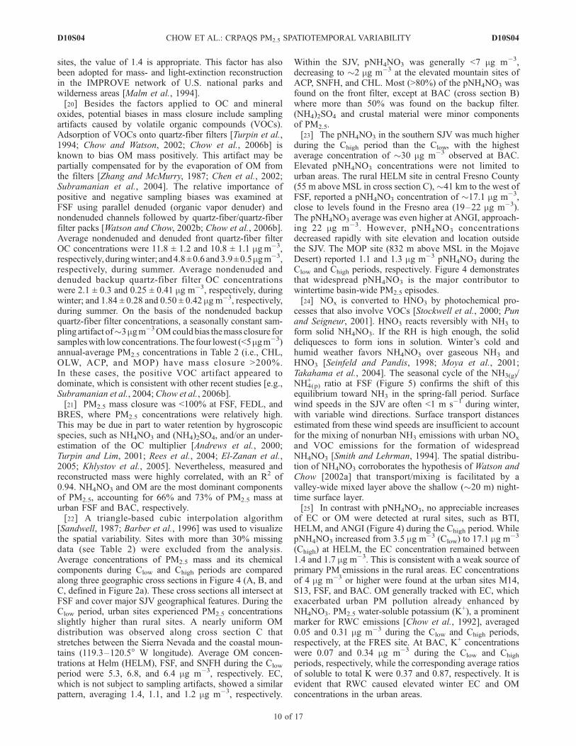
[Sandwell, 1987; Barber et al., 1996] was used to visualizethe spatial variability. Sites with more than 30% missingdata (see Table 2) were excluded from the analysis.Average concentrations of PM2.5 mass and its chemicalcomponents during Clow and Chigh periods are comparedalong three geographic cross sections in Figure 4 (A, B, andC, defined in Figure 2a). These cross sections all intersect atFSF and cover major SJV geographical features. During theClow period, urban sites experienced PM2.5 concentrationsslightly higher than rural sites. A nearly uniform OMdistribution was observed along cross section C thatstretches between the Sierra Nevada and the coastal moun-tains (119.3–120.5� W longitude). Average OM concen-trations at Helm (HELM), FSF, and SNFH during the Clow

period were 5.3, 6.8, and 6.4 mg m�3, respectively. EC,which is not subject to sampling artifacts, showed a similarpattern, averaging 1.4, 1.1, and 1.2 mg m�3, respectively.

Within the SJV, pNH4NO3 was generally <7 mg m�3,decreasing to �2 mg m�3 at the elevated mountain sites ofACP, SNFH, and CHL. Most (>80%) of the pNH4NO3 wasfound on the front filter, except at BAC (cross section B)where more than 50% was found on the backup filter.(NH4)2SO4 and crustal material were minor componentsof PM2.5.[23] The pNH4NO3 in the southern SJV was much higher

during the Chigh period than the Clow, with the highestaverage concentration of �30 mg m�3 observed at BAC.Elevated pNH4NO3 concentrations were not limited tourban areas. The rural HELM site in central Fresno County(55 m above MSL in cross section C),�41 km to the west ofFSF, reported a pNH4NO3 concentration of �17.1 mg m�3,close to levels found in the Fresno area (19–22 mg m�3).The pNH4NO3 average was even higher at ANGI, approach-ing 22 mg m�3. However, pNH4NO3 concentrationsdecreased rapidly with site elevation and location outsidethe SJV. The MOP site (832 m above MSL in the MojaveDesert) reported 1.1 and 1.3 mg m�3 pNH4NO3 during theClow and Chigh periods, respectively. Figure 4 demonstratesthat widespread pNH4NO3 is the major contributor towintertime basin-wide PM2.5 episodes.[24] NOx is converted to HNO3 by photochemical pro-

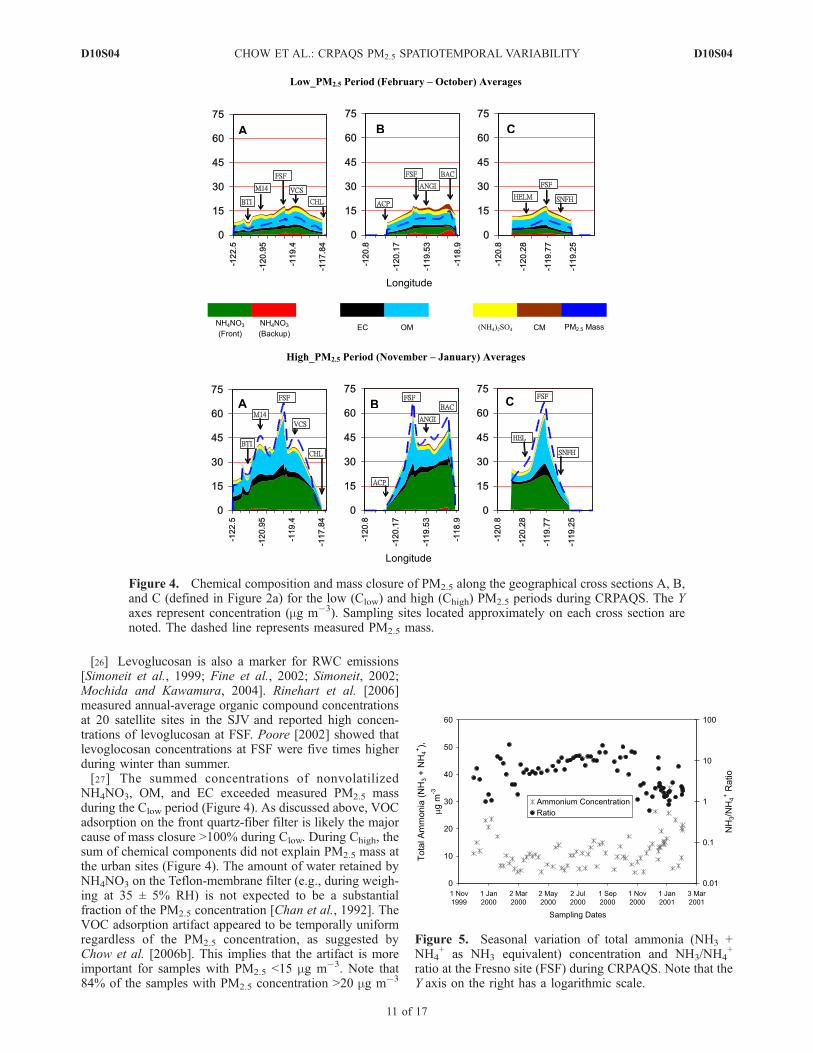
cesses that also involve VOCs [Stockwell et al., 2000; Punand Seigneur, 2001]. HNO3 reacts reversibly with NH3 toform solid NH4NO3. If the RH is high enough, the soliddeliquesces to form ions in solution. Winter’s cold andhumid weather favors NH4NO3 over gaseous NH3 andHNO3 [Seinfeld and Pandis, 1998; Moya et al., 2001;Takahama et al., 2004]. The seasonal cycle of the NH3(g)/NH4

+(p) ratio at FSF (Figure 5) confirms the shift of this

equilibrium toward NH3 in the spring-fall period. Surfacewind speeds in the SJV are often <1 m s�1 during winter,with variable wind directions. Surface transport distancesestimated from these wind speeds are insufficient to accountfor the mixing of nonurban NH3 emissions with urban NOx

and VOC emissions for the formation of widespreadNH4NO3 [Smith and Lehrman, 1994]. The spatial distribu-tion of NH4NO3 corroborates the hypothesis of Watson andChow [2002a] that transport/mixing is facilitated by avalley-wide mixed layer above the shallow (�20 m) night-time surface layer.[25] In contrast with pNH4NO3, no appreciable increases

of EC or OM were detected at rural sites, such as BTI,HELM, and ANGI (Figure 4) during the Chigh period. WhilepNH4NO3 increased from 3.5 mg m�3 (Clow) to 17.1 mg m

�3

(Chigh) at HELM, the EC concentration remained between1.4 and 1.7 mg m�3. This is consistent with a weak source ofprimary PM emissions in the rural areas. EC concentrationsof 4 mg m�3 or higher were found at the urban sites M14,S13, FSF, and BAC. OM generally tracked with EC, whichexacerbated urban PM pollution already enhanced byNH4NO3. PM2.5 water-soluble potassium (K+), a prominentmarker for RWC emissions [Chow et al., 1992], averaged0.05 and 0.31 mg m�3 during the Clow and Chigh periods,respectively, at the FRES site. At BAC, K+ concentrationswere 0.07 and 0.34 mg m�3 during the Clow and Chigh

periods, respectively, while the corresponding average ratiosof soluble to total K were 0.37 and 0.87, respectively. It isevident that RWC caused elevated winter EC and OMconcentrations in the urban areas.


10 of 17

D10S04

[26] Levoglucosan is also a marker for RWC emissions[Simoneit et al., 1999; Fine et al., 2002; Simoneit, 2002;Mochida and Kawamura, 2004]. Rinehart et al. [2006]measured annual-average organic compound concentrationsat 20 satellite sites in the SJV and reported high concen-trations of levoglucosan at FSF. Poore [2002] showed thatlevoglocosan concentrations at FSF were five times higherduring winter than summer.[27] The summed concentrations of nonvolatilized

NH4NO3, OM, and EC exceeded measured PM2.5 massduring the Clow period (Figure 4). As discussed above, VOCadsorption on the front quartz-fiber filter is likely the majorcause of mass closure >100% during Clow. During Chigh, thesum of chemical components did not explain PM2.5 mass atthe urban sites (Figure 4). The amount of water retained byNH4NO3 on the Teflon-membrane filter (e.g., during weigh-ing at 35 ± 5% RH) is not expected to be a substantialfraction of the PM2.5 concentration [Chan et al., 1992]. TheVOC adsorption artifact appeared to be temporally uniformregardless of the PM2.5 concentration, as suggested byChow et al. [2006b]. This implies that the artifact is moreimportant for samples with PM2.5 <15 mg m�3. Note that84% of the samples with PM2.5 concentration >20 mg m�3

Figure 4. Chemical composition and mass closure of PM2.5 along the geographical cross sections A, B,and C (defined in Figure 2a) for the low (Clow) and high (Chigh) PM2.5 periods during CRPAQS. The Yaxes represent concentration (mg m�3). Sampling sites located approximately on each cross section arenoted. The dashed line represents measured PM2.5 mass.

Figure 5. Seasonal variation of total ammonia (NH3 +NH4

+ as NH3 equivalent) concentration and NH3/NH4+

ratio at the Fresno site (FSF) during CRPAQS. Note that theY axis on the right has a logarithmic scale.


11 of 17

D10S04

showed mass closure at <110% regardless of the site; wellwithin the ±10% measurement uncertainties of the PM2.5

mass.

5. Winter PM2.5 Episodes

[28] The winter IOPs were selected from boundary layerstability forecasts, which were based on meteorologicalcharacteristics in the SJV (mixing height, wind speed, andRH) normally associated with high PM2.5 concentrations.The selected four IOP periods are listed in Table 1. Five

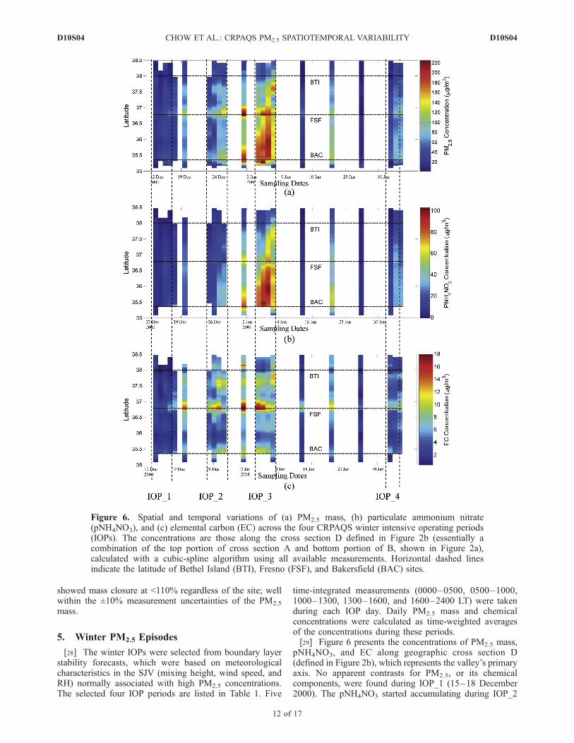
time-integrated measurements (0000–0500, 0500–1000,1000–1300, 1300–1600, and 1600–2400 LT) were takenduring each IOP day. Daily PM2.5 mass and chemicalconcentrations were calculated as time-weighted averagesof the concentrations during these periods.[29] Figure 6 presents the concentrations of PM2.5 mass,

pNH4NO3, and EC along geographic cross section D(defined in Figure 2b), which represents the valley’s primaryaxis. No apparent contrasts for PM2.5, or its chemicalcomponents, were found during IOP_1 (15–18 December2000). The pNH4NO3 started accumulating during IOP_2

Figure 6. Spatial and temporal variations of (a) PM2.5 mass, (b) particulate ammonium nitrate(pNH4NO3), and (c) elemental carbon (EC) across the four CRPAQS winter intensive operating periods(IOPs). The concentrations are those along the cross section D defined in Figure 2b (essentially acombination of the top portion of cross section A and bottom portion of B, shown in Figure 2a),calculated with a cubic-spline algorithm using all available measurements. Horizontal dashed linesindicate the latitude of Bethel Island (BTI), Fresno (FSF), and Bakersfield (BAC) sites.


12 of 17

D10S04

(26 December 2000) in the southern SJV and appeared topersist through early January 2001. High EC (>10 mg m�3)was also observed around urban centers such as M14, FSF,and BAC.[30] A major PM2.5 episode driven by pNH3NO3 oc-

curred during IOP_3 (4–7 January 2001). From IOP_2through IOP_3, the SJV was situated between a persistenthigh-pressure ridge over the Great Basin and a surface lowoff the southern California coast. On 4 January 2001,pNH3NO3 in the southern SJV was 75 mg m�3, and by 5January 2001, this plume blanketed a broad region betweenBAC and FSF. The highest 24-hour average pNH4NO3

concentration of this episode (83 mg m�3) was measuredat ANGI on 6 January 2001. For the first time duringwinter,M14 recorded a pNH4NO3 concentration approaching60 mg m�3 (6–7 January 2001). While pNH4NO3 graduallydissipated in the southern SJV after 6 January 2001,the northern boundary BTI site reported a pNH4NO3

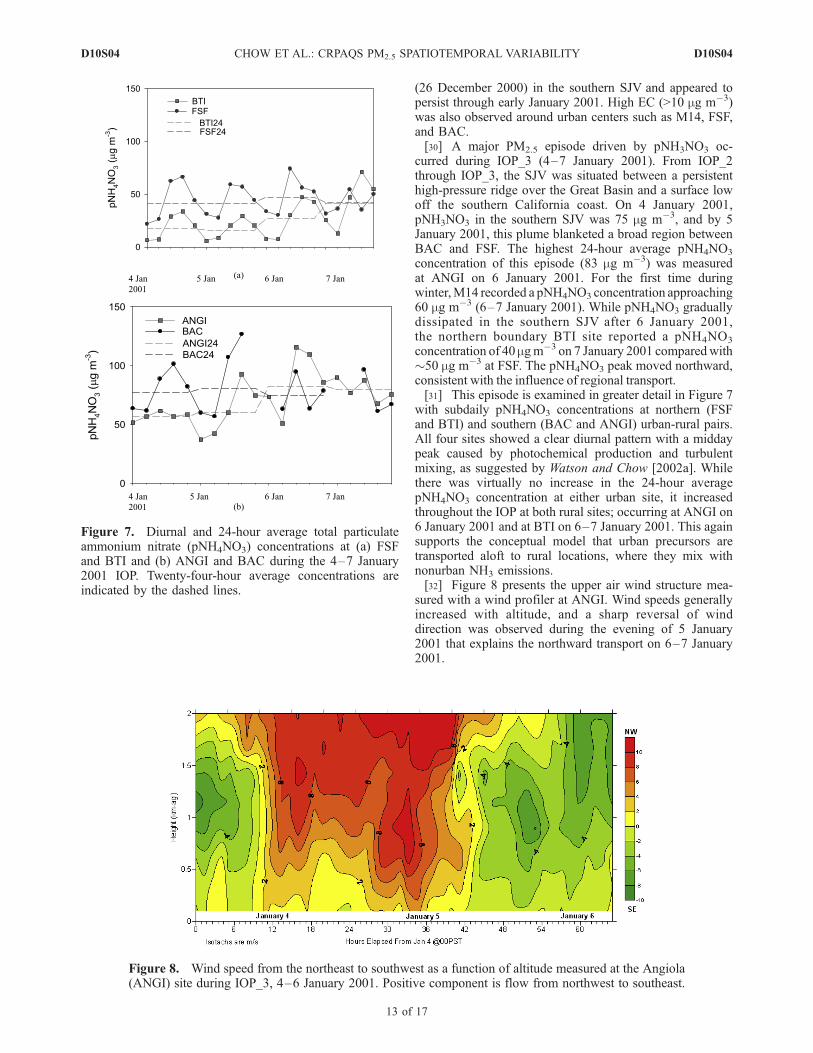
concentration of 40 mgm�3 on 7 January 2001 comparedwith�50 mg m�3 at FSF. The pNH4NO3 peak moved northward,consistent with the influence of regional transport.[31] This episode is examined in greater detail in Figure 7

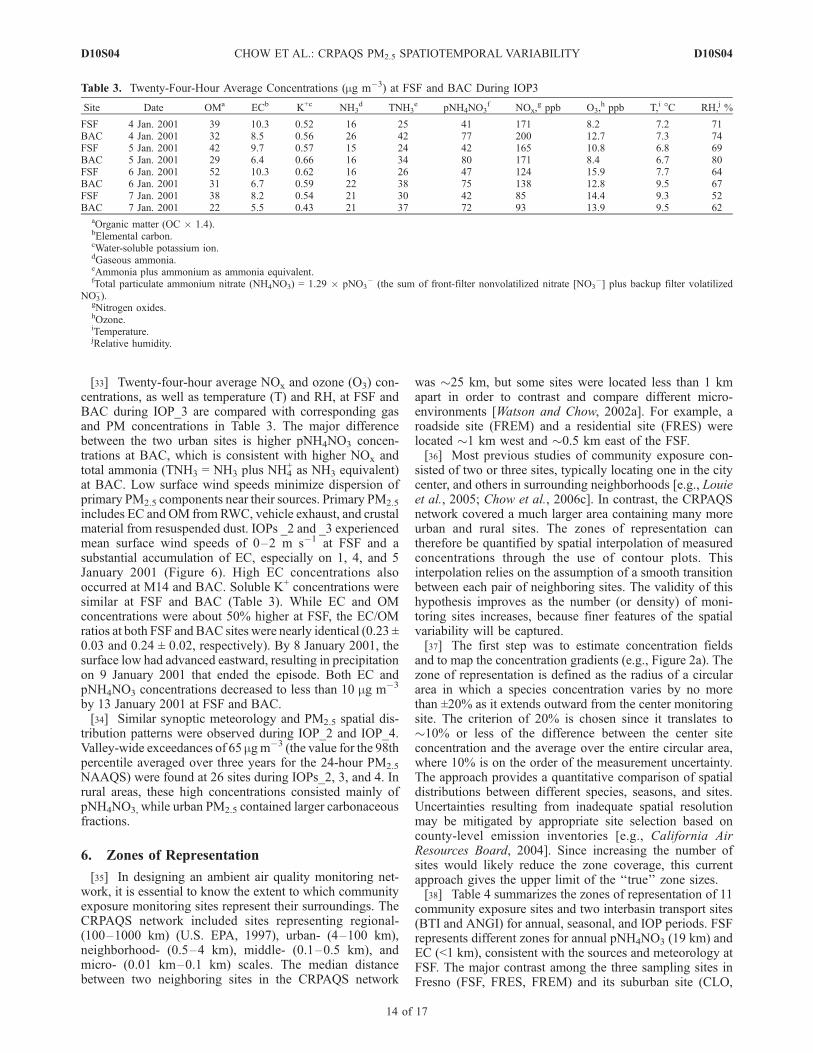
with subdaily pNH4NO3 concentrations at northern (FSFand BTI) and southern (BAC and ANGI) urban-rural pairs.All four sites showed a clear diurnal pattern with a middaypeak caused by photochemical production and turbulentmixing, as suggested by Watson and Chow [2002a]. Whilethere was virtually no increase in the 24-hour averagepNH4NO3 concentration at either urban site, it increasedthroughout the IOP at both rural sites; occurring at ANGI on6 January 2001 and at BTI on 6–7 January 2001. This againsupports the conceptual model that urban precursors aretransported aloft to rural locations, where they mix withnonurban NH3 emissions.[32] Figure 8 presents the upper air wind structure mea-

sured with a wind profiler at ANGI. Wind speeds generallyincreased with altitude, and a sharp reversal of winddirection was observed during the evening of 5 January2001 that explains the northward transport on 6–7 January2001.

Figure 7. Diurnal and 24-hour average total particulateammonium nitrate (pNH4NO3) concentrations at (a) FSFand BTI and (b) ANGI and BAC during the 4–7 January2001 IOP. Twenty-four-hour average concentrations areindicated by the dashed lines.

Figure 8. Wind speed from the northeast to southwest as a function of altitude measured at the Angiola(ANGI) site during IOP_3, 4–6 January 2001. Positive component is flow from northwest to southeast.


13 of 17

D10S04

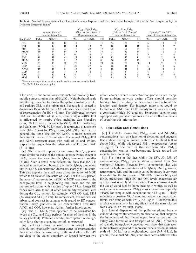
[33] Twenty-four-hour average NOx and ozone (O3) con-centrations, as well as temperature (T) and RH, at FSF andBAC during IOP_3 are compared with corresponding gasand PM concentrations in Table 3. The major differencebetween the two urban sites is higher pNH4NO3 concen-trations at BAC, which is consistent with higher NOx andtotal ammonia (TNH3 = NH3 plus NH4

+ as NH3 equivalent)at BAC. Low surface wind speeds minimize dispersion ofprimary PM2.5 components near their sources. Primary PM2.5

includes EC and OM from RWC, vehicle exhaust, and crustalmaterial from resuspended dust. IOPs _2 and _3 experiencedmean surface wind speeds of 0–2 m s�1 at FSF and asubstantial accumulation of EC, especially on 1, 4, and 5January 2001 (Figure 6). High EC concentrations alsooccurred at M14 and BAC. Soluble K+ concentrations weresimilar at FSF and BAC (Table 3). While EC and OMconcentrations were about 50% higher at FSF, the EC/OMratios at both FSF and BAC sites were nearly identical (0.23 ±0.03 and 0.24 ± 0.02, respectively). By 8 January 2001, thesurface low had advanced eastward, resulting in precipitationon 9 January 2001 that ended the episode. Both EC andpNH4NO3 concentrations decreased to less than 10 mg m�3

by 13 January 2001 at FSF and BAC.[34] Similar synoptic meteorology and PM2.5 spatial dis-

tribution patterns were observed during IOP_2 and IOP_4.Valley-wide exceedances of 65 mgm�3 (the value for the 98thpercentile averaged over three years for the 24-hour PM2.5

NAAQS) were found at 26 sites during IOPs_2, 3, and 4. Inrural areas, these high concentrations consisted mainly ofpNH4NO3, while urban PM2.5 contained larger carbonaceousfractions.

6. Zones of Representation

[35] In designing an ambient air quality monitoring net-work, it is essential to know the extent to which communityexposure monitoring sites represent their surroundings. TheCRPAQS network included sites representing regional-(100–1000 km) (U.S. EPA, 1997), urban- (4–100 km),neighborhood- (0.5–4 km), middle- (0.1–0.5 km), andmicro- (0.01 km–0.1 km) scales. The median distancebetween two neighboring sites in the CRPAQS network

was �25 km, but some sites were located less than 1 kmapart in order to contrast and compare different micro-environments [Watson and Chow, 2002a]. For example, aroadside site (FREM) and a residential site (FRES) werelocated �1 km west and �0.5 km east of the FSF.[36] Most previous studies of community exposure con-

sisted of two or three sites, typically locating one in the citycenter, and others in surrounding neighborhoods [e.g., Louieet al., 2005; Chow et al., 2006c]. In contrast, the CRPAQSnetwork covered a much larger area containing many moreurban and rural sites. The zones of representation cantherefore be quantified by spatial interpolation of measuredconcentrations through the use of contour plots. Thisinterpolation relies on the assumption of a smooth transitionbetween each pair of neighboring sites. The validity of thishypothesis improves as the number (or density) of moni-toring sites increases, because finer features of the spatialvariability will be captured.[37] The first step was to estimate concentration fields

and to map the concentration gradients (e.g., Figure 2a). Thezone of representation is defined as the radius of a circulararea in which a species concentration varies by no morethan ±20% as it extends outward from the center monitoringsite. The criterion of 20% is chosen since it translates to�10% or less of the difference between the center siteconcentration and the average over the entire circular area,where 10% is on the order of the measurement uncertainty.The approach provides a quantitative comparison of spatialdistributions between different species, seasons, and sites.Uncertainties resulting from inadequate spatial resolutionmay be mitigated by appropriate site selection based oncounty-level emission inventories [e.g., California AirResources Board, 2004]. Since increasing the number ofsites would likely reduce the zone coverage, this currentapproach gives the upper limit of the ‘‘true’’ zone sizes.[38] Table 4 summarizes the zones of representation of 11

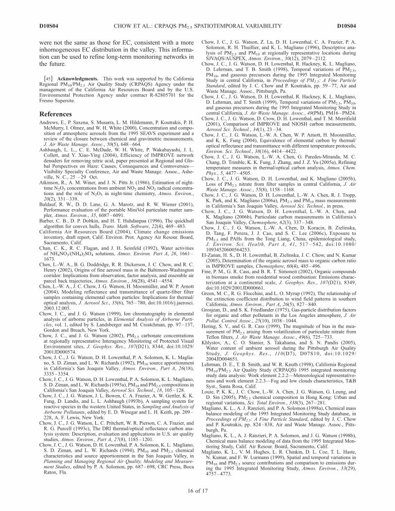
community exposure sites and two interbasin transport sites(BTI and ANGI) for annual, seasonal, and IOP periods. FSFrepresents different zones for annual pNH4NO3 (19 km) andEC (<1 km), consistent with the sources and meteorology atFSF. The major contrast among the three sampling sites inFresno (FSF, FRES, FREM) and its suburban site (CLO,

Table 3. Twenty-Four-Hour Average Concentrations (mg m�3) at FSF and BAC During IOP3

Site Date OMa ECb K+c NH3d TNH3

e pNH4NO3f NOx,

g ppb O3,h ppb T,i �C RH,j %

FSF 4 Jan. 2001 39 10.3 0.52 16 25 41 171 8.2 7.2 71BAC 4 Jan. 2001 32 8.5 0.56 26 42 77 200 12.7 7.3 74FSF 5 Jan. 2001 42 9.7 0.57 15 24 42 165 10.8 6.8 69BAC 5 Jan. 2001 29 6.4 0.66 16 34 80 171 8.4 6.7 80FSF 6 Jan. 2001 52 10.3 0.62 16 26 47 124 15.9 7.7 64BAC 6 Jan. 2001 31 6.7 0.59 22 38 75 138 12.8 9.5 67FSF 7 Jan. 2001 38 8.2 0.54 21 30 42 85 14.4 9.3 52BAC 7 Jan. 2001 22 5.5 0.43 21 37 72 93 13.9 9.5 62

aOrganic matter (OC � 1.4).bElemental carbon.cWater-soluble potassium ion.dGaseous ammonia.eAmmonia plus ammonium as ammonia equivalent.fTotal particulate ammonium nitrate (NH4NO3) = 1.29 � pNO3

� (the sum of front-filter nonvolatilized nitrate [NO3�] plus backup filter volatilized

NO3�).gNitrogen oxides.hOzone.iTemperature.jRelative humidity.


14 of 17

D10S04

7 km east) is due to carbonaceous material, probably frommobile sources, rather than pNH4NO3. Neighborhood-scalemonitoring is needed to resolve the spatial variability of EC,and perhaps OM, in this urban area. Because it is located indowntown Bakersfield, the BAC site also has a small zoneof representation for EC (�1 km). The difference betweenBAC and its satellite site (BRES, 2 km west) is �40%. BTIis influenced by nearby cities, including San Francisco(SFA, 70 km west), Sacramento (S13, 50 km northeast),and Stockton (SOH, 30 km east). It represents a consistentzone (10–15 km) for PM2.5 mass, pNH4NO3, and EC. Ingeneral, the zone size for pNH4NO3 is more consistentthan for EC across different sites. For annual PM2.5, BTIand ANGI represent areas with radii of 15 and 19 km,respectively, larger than the urban sites of FSF and BAC(7–11 km).[39] The zones of representation during the Chigh period

were similar to those of the annual-average zones except atBAC, where the zone for pNH4NO3 was much smaller(3 km). Such a small zone reflects the facts that BAC islocated at the southern boundary of the NH4NO3 plume andthat NH4NO3 concentration decreases sharply to the south.This also explains the small zone of representation of MOP,which is an elevated site south of BAC. For the Clow period,the zone of representation of EC at MOP was close to thebackground level in neighboring rural areas and this siterepresented a zone with a radius of up to 55 km. Larger ECzones were also found at other community exposure sitesduring the Clow period; for example, VCS (30 km), M14(34 km), and S13 (37 km). To some extent, this reflects lessurban-rural contrast in summer with regard to EC concen-tration. Sharp gradients in EC concentration near ruralANGI and COP, however, warrant further investigation.[40] The pNH4NO3 zone appeared to be consistent be-

tween the Clow and Chigh periods for most of the sites in thevalley (Table 4). Pollutants exhibit more spatial inhomoge-neity for a shorter averaging period, as expected.[41] Factors affecting the zone size are complex. Rural

sites do not necessarily have larger zones of representationthan urban sites, because many of the rural sites in the SJVare close to the valley boundary, or located between two

urban centers where concentration gradients are steep.Future ambient network design efforts should considerfindings from this study to determine more optimal sitelocation and density. For instance, more sites could belocated near ANGI and COP (mainly to the west) to verifya consistently high EC gradient. Temporary satellite sitesequipped with portable monitors are a cost effective meansof acquiring this information.

7. Discussion and Conclusions

[42] CRPAQS shows that PM2.5 mass and NH4NO3

concentrations vary as a function of elevation, and suggeststhat vertical mixing is limited in the SJV to about 600 mabove MSL. While widespread PM2.5 exceedances (up to30 mg m�3) occurred in the southern SJV, PM2.5

concentration was at near-background levels toward themountainous boundary.[43] For most of the sites within the SJV, 50–75% of

annual-average PM2.5 concentrations occurred from No-vember to January. Elevated PM2.5 at nonurban sites wascaused by high concentrations of NH4NO3. During winter,temperature, RH, and the stable valley boundary layer werefavorable for the formation of NH4NO3 from its NH3 andHNO3 precursors. High EC and OM levels exacerbate airquality most severely at urban sites. This is consistent withthe use of wood fuel for home heating in winter, as well asmotor vehicle emissions. PM2.5 mass closure was typically>100% for samples with concentrations <15 mg m�3, likelyreflecting a positive VOC sampling artifact on quartz-fiberfilters. For samples with PM2.5 >20 mg m�3, however, thisartifact was relatively less significant and the mass closurewas close to, or less than, 100%.[44] Lateral dispersion of the pollution plume became

evident during winter episodes, an observation that supportsthe hypothesis of the role of upper layer currents on thevalley-wide formation and transport of NH4NO3. Gradientsof spatially interpolated concentrations show that most sitesin the network appeared to represent zone sizes on an urbanscale (4–100 km) or a neighborhood scale (0.5–4 km). Ingeneral, the annual NH4NO3 zone sizes across different sites

Table 4. Zone of Representation for Eleven Community Exposure and Two Interbasin Transport Sites in the San Joaquin Valley on

Different Temporal Scalesa

Site Codeb

Annual: Zone ofRepresentation, km

Chigh: High_PM2.5

(Nov. to Jan.): Zone ofRepresentation, km

Clow: Low_PM2.5

(Feb. to Oct.): Zone ofRepresentation, km

Episode (7 Jan. 2001):Zone of Representation, km

PM2.5 pNH4NO3 EC PM2.5 pNH4NO3 EC PM2.5 pNH4NO3 EC PM2.5 pNH4NO3 EC

S13 12 12 12 10 11 11 54 31 37 6 10 15BTI 15 13 10 14 10 9 15 16 10 5 10 9M14 22 20 23 19 20 17 25 20 34 6 18 12MRM 19 14 14 15 14 13 27 15 14 1 12 11CLO 6 10 3 6 10 3 9 11 3 5 4 4FSF 11 19 <1 10 18 <1 13 12 1 11 2 8SELM 13 21 9 12 19 8 20 23 12 1 10 12VCS 23 19 28 21 18 23 28 21 30 14 9 16COP 22 23 6 21 27 6 16 16 6 5 18 6ANGI 19 19 4 19 19 4 16 16 3 12 14 4OLD 6 21 4 15 12 3 3 5 7 8 14 3BAC 7 12 1 4 3 2 5 8 6 6 5 4MOP 8 3 20 3 1 7 15 8 55 14 1 10aSites are arranged from north to south; anchor sites are noted in bold.bSee Table 1 for site description.


15 of 17

D10S04

were not the same as those for EC, consistent with a moreinhomogeneous EC distribution in the valley. This informa-tion can be used to refine long-term monitoring networks inthe future.

[45] Acknowledgments. This work was supported by the CaliforniaRegional PM10/PM2.5 Air Quality Study (CRPAQS) Agency under themanagement of the California Air Resources Board and by the U.S.Environmental Protection Agency under contract R-82805701 for theFresno Supersite.

ReferencesAndrews, E., P. Saxena, S. Musarra, L. M. Hildemann, P. Koutrakis, P. H.McMurry, I. Olmez, and W. H. White (2000), Concentration and compo-sition of atmospheric aerosols from the 1995 SEAVS experiment and areview of the closure between chemical and gravimetric measurements,J. Air Waste Manage. Assoc., 50(5), 648–664.

Ashbaugh, L. L., C. E. McDade, W. H. White, P. Wakabayashi, J. L.Collett, and Y. Xiao-Ying (2004), Efficiency of IMPROVE networkdenuders for removing nitric acid, paper presented at Regional and Glo-bal Perspectives on Haze: Causes, Consequences and Controversies—Visibility Specialty Conference, Air and Waste Manage. Assoc., Ashe-ville, N. C., 25 –29 Oct.

Atkinson, R., A. M. Winer, and J. N. Pitts Jr. (1986), Estimation of night-time N2O5 concentrations from ambient NO2 and NO3 radical concentra-tions and the role of N2O5 in night-time chemistry, Atmos. Environ.,20(2), 331–339.

Baldauf, R. W., D. D. Lane, G. A. Marotz, and R. W. Wiener (2001),Performance evaluation of the portable MiniVol particulate matter sam-pler, Atmos. Environ., 35, 6087–6091.

Barber, C. B., D. P. Dobkin, and H. T. Huhdanpaa (1996), The quickhullalgorithm for convex hulls, Trans. Math. Software, 22(4), 469–483.

California Air Resources Board (2004), Climate change emissionsinventory, draft report, Calif. Environ. Prot. Agency Air Resour. Board,Sacramento, Calif.

Chan, C. K., R. C. Flagan, and J. H. Seinfeld (1992), Water activitiesof NH4NO3/(NH4)2SO4 solutions, Atmos. Environ. Part A, 26, 1661–1673.

Chen, L.-W. A., B. G. Doddridge, R. R. Dickerson, J. C. Chow, and R. C.Henry (2002), Origins of fine aerosol mass in the Baltimore-Washingtoncorridor: Implications from observation, factor analysis, and ensemble airparcel back trajectories, Atmos. Environ., 36(28), 4541–4554.

Chen, L.-W. A., J. C. Chow, J. G. Watson, H. Moosmuller, and W. P. Arnott(2004), Modeling reflectance and transmittance of quartz-fiber filtersamples containing elemental carbon particles: Implications for thermal/optical analysis, J. Aerosol Sci., 35(6), 765–780, doi:10.1016/j.jaerosci.2003.12.005.

Chow, J. C., and J. G. Watson (1999), Ion chromatography in elementalanalysis of airborne particles, in Elemental Analysis of Airborne Parti-cles, vol. 1, edited by S. Landsberger and M. Creatchman, pp. 97–137,Gordon and Breach, New York.

Chow, J. C., and J. G. Watson (2002), PM2.5 carbonate concentrationsat regionally representative Interagency Monitoring of Protected VisualEnvironment sites, J. Geophys. Res., 107(D21), 8344, doi:10.1029/2001JD000574.

Chow, J. C., J. G. Watson, D. H. Lowenthal, P. A. Solomon, K. L. Maglia-no, S. D. Ziman, and L. W. Richards (1992), PM10 source apportionmentin California’s San Joaquin Valley, Atmos. Environ., Part A, 26(18),3335–3354.

Chow, J. C., J. G. Watson, D. H. Lowenthal, P. A. Solomon, K. L. Magliano,S. D. Ziman, and L.W. Richards (1993a), PM10 and PM2.5 compositions inCalifornia’s San Joaquin Valley, Aerosol Sci. Technol., 18, 105–128.

Chow, J. C., J. G. Watson, J. L. Bowen, C. A. Frazier, A. W. Gertler, K. K.Fung, D. Landis, and L. L. Ashbaugh (1993b), A sampling system forreactive species in the western United States, in Sampling and Analysis ofAirborne Pollutants, edited by E. D. Winegar and L. H. Keith, pp. 209–228, A. F. Lewis, New York.

Chow, J. C., J. G. Watson, L. C. Pritchett, W. R. Pierson, C. A. Frazier, andR. G. Purcell (1993c), The DRI thermal/optical reflectance carbon ana-lysis system: Description, evaluation and applications in U.S. air qualitystudies, Atmos. Environ., Part A, 27(8), 1185–1201.

Chow, J. C., J. G. Watson, D. H. Lowenthal, P. A. Solomon, K. L. Magliano,S. D. Ziman, and L. W. Richards (1994), PM10 and PM2.5 chemicalcharacteristics and source apportionment in the San Joaquin Valley, inPlanning and Managing Regional Air Quality, Modeling and Measure-ment Studies, edited by P. A. Solomon, pp. 687–698, CRC Press, BocaRaton, Fla.

Chow, J. C., J. G. Watson, Z. Lu, D. H. Lowenthal, C. A. Frazier, P. A.Solomon, R. H. Thuillier, and K. L. Magliano (1996), Descriptive ana-lysis of PM2.5 and PM10 at regionally representative locations duringSJVAQS/AUSPEX, Atmos. Environ., 30(12), 2079–2112.

Chow, J. C., J. G. Watson, D. H. Lowenthal, R. Hackney, K. L. Magliano,D. Lehrman, and T. B. Smith (1998), Temporal variations of PM2.5,PM10, and gaseous precursors during the 1995 Integrated MonitoringStudy in central California, in Proceedings of PM2.5: A Fine ParticleStandard, edited by J. C. Chow and P. Koutrakis, pp. 59–77, Air andWaste Manage. Assoc., Pittsburgh, Pa.

Chow, J. C., J. G. Watson, D. H. Lowenthal, R. Hackney, K. L. Magliano,D. Lehrman, and T. Smith (1999), Temporal variations of PM2.5, PM10,and gaseous precursors during the 1995 Integrated Monitoring Study incentral California, J. Air Waste Manage. Assoc., 49(PM), PM16–PM24.

Chow, J. C., J. G. Watson, D. Crow, D. H. Lowenthal, and T. M. Merrifield(2001), Comparison of IMPROVE and NIOSH carbon measurements,Aerosol Sci. Technol., 34(1), 23–34.

Chow, J. C., J. G. Watson, L.-W. A. Chen, W. P. Arnott, H. Moosmuller,and K. K. Fung (2004), Equivalence of elemental carbon by thermal/optical reflectance and transmittance with different temperature protocols,Environ. Sci. Technol., 38(16), 4414–4422.

Chow, J. C., J. G. Watson, L.-W. A. Chen, G. Paredes-Miranda, M. C.Chang, D. Trimble, K. K. Fung, J. Zhang, and J. Z. Yu (2005a), Refiningtemperature measures in thermal/optical carbon analysis, Atmos. Chem.Phys., 5, 4477–4505.

Chow, J. C., J. G. Watson, D. H. Lowenthal, and K. Magliano (2005b),Loss of PM2.5 nitrate from filter samples in central California, J. AirWaste Manage. Assoc., 55(8), 1158–1168.

Chow, J. C., J. G. Watson, D. H. Lowenthal, L.-W. A. Chen, R. J. Tropp,K. Park, and K. Magliano (2006a), PM2.5 and PM10 mass measurementsin California’s San Joaquin Valley, Aerosol Sci. Technol., in press.

Chow, J. C., J. G. Watson, D. H. Lowenthal, L.-W. A. Chen, andK. Magliano (2006b), Particulate carbon measurements in California’sSan Joaquin Valley, Chemosphere, 62(3), 337–348.

Chow, J. C., J. G. Watson, L.-W. A. Chen, D. Koracin, B. Zielinska,D. Tang, F. Perera, J. J. Cao, and S. C. Lee (2006c), Exposure toPM2.5 and PAHs from the Tong Liang, China, epidemiological study,J. Environ. Sci. Health, Part A, 41, 517 – 542, doi:10.1080/10934520600564253.

El-Zanan, H. S., D. H. Lowenthal, B. Zielinska, J. C. Chow, and N. Kumar(2005), Determination of the organic aerosol mass to organic carbon ratioin IMPROVE samples, Chemosphere, 60(4), 485–496.

Fine, P. M., G. R. Cass, and B. R. T. Simoneit (2002), Organic compoundsin biomass smoke from residential wood combustion: Emissions charac-terization at a continental scale, J. Geophys. Res., 107(D21), 8349,doi:10.1029/2001JD000661.

Green, M. C., R. G. Flocchini, and L. O. Myrup (1992), The relationship ofthe extinction coefficient distribution to wind field patterns in southernCalifornia, Atmos. Environ., Part A, 26(5), 827–840.

Grosjean, D., and S. K. Friedlander (1975), Gas-particle distribution factorsfor organic and other pollutants in the Los Angeles atmosphere, J. AirPollut. Control Assoc., 25(10), 1038–1044.

Hering, S. V., and G. R. Cass (1999), The magnitude of bias in the mea-surement of PM2.5 arising from volatilization of particulate nitrate fromTeflon filters, J. Air Waste Manage. Assoc., 49(6), 725–733.

Khlystov, A., C. O. Stanier, S. Takahama, and S. N. Pandis (2005),Water content of ambient aerosol during the Pittsburgh Air QualityStudy, J. Geophys. Res. , 110(D7), D07S10, doi:10.1029/2004JD004651.

Lehrman, D. E., T. B. Smith, and W. R. Knuth (1998), California RegionalPM10/PM2.5 Air Quality Study (CRPAQS) 1995 integrated monitoringstudy data analysis: Work element 2.2.2—Meteorological representative-ness and work element 2.2.3—Fog and low clouds characteristics, T&BSyst., Santa Rosa, Calif.

Louie, P. K. K., J. C. Chow, L.-W. A. Chen, J. G. Watson, G. Leung, andD. Sin (2005), PM2.5 chemical composition in Hong Kong: Urban andregional variations, Sci. Total Environ., 338(3), 267–281.

Magliano, K. L., A. J. Ranzieri, and P. A. Solomon (1998a), Chemical massbalance modeling of the 1995 Integrated Monitoring Study database, inProceedings of PM2.5: A Fine Particle Standard, edited by J. C. Chowand P. Koutrakis, pp. 824–838, Air and Waste Manage. Assoc., Pitts-burgh, Pa.

Magliano, K. L., A. J. Ranzieri, P. A. Solomon, and J. G. Watson (1998b),Chemical mass balance modeling of data from the 1995 Integrated Mon-itoring Study, Calif. Air Resour. Board, Sacramento, Calif.

Magliano, K. L., V. M. Hughes, L. R. Chinkin, D. L. Coe, T. L. Haste,N. Kumar, and F. W. Lurmann (1999), Spatial and temporal variations inPM10 and PM2.5 source contributions and comparison to emissions dur-ing the 1995 Integrated Monitoring Study, Atmos. Environ., 33(29),4757–4773.


16 of 17

D10S04

Malm, W. C., J. F. Sisler, D. Huffman, R. A. Eldred, and T. A. Cahill(1994), Spatial and seasonal trends in particle concentration and opticalextinction in the United States, J. Geophys. Res., 99(D1), 1347–1370.

Mochida, M., and K. Kawamura (2004), Hygroscopic properties of levo-glucosan and related organic compounds characteristic to biomass burn-ing aerosol particles, J. Geophys. Res., 109, D21202, doi:10.1029/2004JD004962.

Moya, M., A. S. Ansari, and S. N. Pandis (2001), Partitioning of nitrate andammonium between the gas and particulate phases during the 1997 IM-ADA-AVER study in Mexico City, Atmos. Environ., 35(10), 1791–1804.

Poore, M. W. (2002), Levoglucosan in PM2.5 at the Fresno Supersite, J. AirWaste Manage. Assoc., 52(1), 3–4.

Pun, B. K., and C. Seigneur (2001), Sensitivity of particulate matter nitrateformation to precursor emissions in the California San Joaquin Valley,Environ. Sci. Technol., 35(14), 2979–2987.

Rees, S. L., A. L. Robinson, A. Khlystov, C. O. Stanier, and S. N. Pandis(2004), Mass balance closure and the federal reference method for PM2.5

in Pittsburgh, Pennsylvania, Atmos. Environ., 38(20), 3305–3318.Rinehart, L. R., E. M. Fujita, J. C. Chow, K. Magliano, and B. Zielinska(2006), Spatial distribution of PM2.5 associated organic compounds incentral California, Atmos. Environ., 40(2), 290–303.

Russell, L. M. (2003), Aerosol organic-mass-to-organic-carbon ratio mea-surements, Environ. Sci. Technol., 37(13), 2982–2987, doi:10.1021/es026123w.

Sandwell, D. T. (1987), Biharmonic spline interpolation of GEOS-3 andSEASAT altimeter data, Geophys. Res. Lett., 2, 139–142.

Schauer, J. J., and G. R. Cass (2000), Source apportionment of wintertimegas-phase and particle-phase air pollutants using organic compounds astracers, Environ. Sci. Technol., 34(9), 1821–1832.

Seinfeld, J. H., and S. N. Pandis (1998), Atmospheric Chemistry and Phy-sics: From Air Pollution to Climate Change, John Wiley, Hoboken, N. J.

Simoneit, B. R. T. (2002), Chemical characterization of sub-micron organicaerosols in the tropical trade winds of the Caribbean using gas chroma-tography-mass spectrometry, Atmos. Environ., 36(33), 5259–5263.

Simoneit, B. R. T., J. J. Schauer, C. G. Nolte, D. R. Oros, V. O. Elias, M. P.Fraser, W. F. Rogge, and G. R. Cass (1999), Levoglucosan, a tracer forcellulose in biomass burning and atmospheric particles, Atmos. Environ.,33(2), 173–182.

Smith, T. B., and D. E. Lehrman (1994), Long-range tracer studies in theSan Joaquin Valley, in Proceedings of Regional Photochemical Measure-ment and Modeling Studies, vol. 1, edited by A. J. Ranzieri and P. A.Solomon, pp. 151–165, Air and Waste Manage. Assoc., Pittsburgh, Pa.

Stockwell, W. R., J. G. Watson, N. F. Robinson, W. Steiner, and W. W.Sylte (2000), The ammonium nitrate particle equivalent of NOx emis-sions for wintertime conditions in central California’s San Joaquin Valley,Atmos. Environ., 34(27), 4711–4717.

Subramanian, R., A. Y. Khlystov, J. C. Cabada, and A. L. Robinson (2004),Positive and negative artifacts in particulate organic carbon measure-ments with denuded and undenuded sampler configurations, AerosolSci. Technol., 38, suppl. 1, 27–48.

Takahama, S., A. E. Wittig, D. V. Vayenas, C. I. Davidson, and S. N. Pandis(2004), Modeling the diurnal variation of nitrate during the Pittsburgh AirQuality Study, J. Geophys. Res., 109, D16S06, doi:10.1029/2003JD004149.

Turpin, B. J., and H. J. Lim (2001), Species contributions to PM2.5 massconcentrations: Revisiting common assumptions for estimating organicmass, Aerosol Sci. Technol., 35(1), 602–610.

Turpin, B. J., J. J. Huntzicker, and S. V. Hering (1994), Investigation oforganic aerosol sampling artifacts in the Los Angeles basin, Atmos. En-viron., 28(19), 3061–3071.

U.S. Environmental Protection Agency (1997), National ambient air qualitystandards for particulate matter: Final rule, Fed. Regist., 62(138),38,651–38,701.

Watson, J. G., and J. C. Chow (2002a), A wintertime PM2.5 episode at theFresno, CA Supersite, Atmos. Environ., 36(3), 465–475.

Watson, J. G., and J. C. Chow (2002b), Comparison and evaluation of insitu and filter carbon measurements at the Fresno Supersite, J. Geophys.Res., 107(D21), 8341, doi:10.1029/2001JD000573.

Watson, J. G., J. C. Chow, Z. Lu, E. M. Fujita, D. H. Lowenthal, and D. R.Lawson (1994), Chemical mass balance source apportionment of PM10

during the Southern California Air Quality Study, Aerosol Sci. Technol.,21(1), 1–36.

Watson, J. G., P. J. Lioy, and P. K. Mueller (1995), The measurementprocess: Precision, accuracy, and validity, in Air Sampling Instrumentsfor Evaluation of Atmospheric Contaminants, 8th ed., edited by B. S.Cohen and S. V. Hering, pp. 187–194, Am. Conf. of Govt. Ind. Hyg.,Cincinnati, Ohio.

Watson, J. G., D.W. DuBois, R. DeMandel, A. P. Kaduwela, K. L.Magliano,C. McDade, P. K. Mueller, A. J. Ranzieri, P. M. Roth, and S. Tanrikulu(1998), Field program plan for the California Regional PM10/PM2.5 AirQuality Study (CRPAQS), Desert Res. Inst., Reno, Nev.

Watson, J. G., J. C. Chow, J. L. Bowen, D. H. Lowenthal, S. Hering,P. Ouchida, and W. Oslund (2000), Air quality measurements from theFresno Supersite, J. Air Waste Manage. Assoc., 50(8), 1321–1334.

Watson, J. G., J. C. Chow, D. H. Lowenthal, M. R. Stolzenburg, N. M.Kreisberg, and S. V. Hering (2002), Particle size relationships at theFresno Supersite, J. Air Waste Manage. Assoc., 52(7), 822–827.

White, W. H., and P. T. Roberts (1977), On the nature and origins ofvisibility-reducing aerosols in the Los Angeles air basin, Atmos. Environ.,11(9), 803–812.

Zhang, X. Q., and P. H. McMurry (1987), Theoretical analysis of evapora-tive losses from impactor and filter deposits, Atmos. Environ., 21(8),1779–1789.

Zhang, X. Q., and P. H. McMurry (1992), Evaporative losses of fine parti-culate nitrates during sampling, Atmos. Environ., Part A, 26(18), 3305–3312.

��L.-W. A. Chen, J. C. Chow, D. H. Lowenthal, and J. G. Watson, Division

of Atmospheric Sciences, Desert Research Institute, Reno, NV 89512,USA. ([email protected])D. E. Lehrman, Technical and Business Systems, Santa Rosa, CA 95404,

USA.K. A. Magliano and K. Turkiewicz, California Air Resources Board,

Sacramento, CA 95812, USA.


17 of 17

D10S04

Date post:	05-Jun-2018
Category:	Documents
Upload:	phungdien
View:	219 times
Download:	0 times

PM2.5 chemical composition and spatiotemporal variability ...€¦ · PM 2.5 chemical composition...

Documents