PML ENHANCED WITH A SELF-ADAPTIVE GOAL-ORIENTED HPFINITE-ELEMENT METHOD: SIMULATION OF

THROUGH-CASING BOREHOLE RESISTIVITY MEASUREMENTS

D. PARDO, L. DEMKOWICZ, C. TORRES-VERDIN, AND C. MICHLER

Abstract. We describe the application of a Perfectly Matched Layer (PML) combined with aself-adaptive goal-oriented hp Finite Element (FE) method to the simulation of resistivity measure-ments. The adaptive refinements and fast convergence of the self-adaptive hp FE method enhance theperformance of the PML and, thus, enable the accurate and efficient truncation of the computationaldomain in open domain problems. We apply this methodology to the simulation of axisymmetricthrough-casing resistivity measurements in a borehole environment that are typically used for theassessment of rock formation properties. Our numerical results confirm the accuracy and efficiencyof our method and provide evidence of highly accurate and reliable simulations of borehole loggingmeasurements in the presence of a conductive steel casing and material contrast of fourteen ordersof magnitude in conductivity. Moreover, the combination of adaptivity and PML enables us tosignificantly reduce the size of the computational domain.

Key words. hp-Finite Elements, Perfectly Matched Layer (PML), exponential convergence,goal-oriented adaptivity, through-casing resistivity measurements.

1. INTRODUCTION. In 1994, Berenger [3] introduced the concept of a Per-fectly Matched Layer (PML) for exterior electromagnetic problems to reduce reflec-tions from the boundary of a truncated computational domain. During the same year,the concept of PML was recognized as complex-coordinate stretching of Maxwell’sequations by Chew et al. [5], which essentially means that the PML constitutes ananalytic continuation of the governing equations into the complex plane; see also [22].More recent contributions summarizing the mathematical developments and insightinto PMLs can be found in [21, 25].

Let us briefly review the main idea of the PML and the difficulties pertainingto its implementation. Within the PML, both propagating and evanescent wavesare transformed into evanescent waves with fast exponential decay. Thus, on theouter boundary of the PML, waves are highly attenuated in magnitude such thatreflections due to an ad-hoc boundary condition (BC) (for example, a homogeneousDirichlet boundary condition) become negligible. Since the exponential decay of thewaves within the PML can be made arbitrarily large, reflections from the PML canbe made arbitrarily small. However, the rapid decay of the solution in the PMLproduces a “boundary layer”. Note that the resolution of such PML-induced boundarylayers is crucial for the accuracy of the solution. Failing to ensure a sufficiently finediscretization in the PML typically results in spurious reflections that contaminatethe solution in the entire computational domain.

Conventional discretization methods face a trade-off between using a highly at-tenuating PML that minimizes reflections and a PML with low attenuation that istypically easier to resolve. The more a wave is attenuated within the PML, the smallerare the reflections from the truncated domain boundary provided that the discretiza-tion can accurately resolve the rapidly changing solution in the PML. On the otherhand, the more the solution is attenuated in the PML, the stronger are the resultinggradients and, hence, the more difficult it is for conventional discretization methodsto provide adequate resolution.

We improve the performance of the PML by combining it with a numerical methodthat is capable of accurately resolving strong boundary layers; see [10] for some fun-damental work on this subject in the context of acoustics, elasticity and electromag-

1

netics. This numerical approach is based on a self-adaptive goal-oriented hp FiniteElement (FE) method that automatically, i.e. without any user interaction, constructsan accurate approximation of boundary layers with relatively few unknowns. The useof this methodology renders the design of sophisticated PMLs unnecessary. We sim-ply select any PML that provides sufficiently high attenuation to eliminate reflectionsfrom the boundary; then, the self-adaptive algorithm automatically produces a gridthat accurately resolves the PML-induced boundary layer. Thus, no tuning of thePML is required.

Here, we apply the PML technique combined with the self-adaptive goal-orientedhp-FEM to problems arising in electromagnetic logging; see [15, 16] for details and val-idation of the adaptive method. To this end, we investigate different PMLs (includingdiscontinuous PMLs) to simulate challenging axisymmetric through-casing resistivitymeasurements in a borehole environment. In this problem, currents propagate longdistances through steel casing. To avoid the use of large computational domains, weemploy the Maxwellian anisotropic PML formulation in cylindrical coordinates de-scribed in [23]. Thus, we significantly reduce the size of the computational domain,thereby eliminating unnecessarily elongated elements. It is important to note thatthe discretization in the PML needs to be highly accurate to avoid reflections frommaterials with a conductivity contrast of up to fourteen orders of magnitude.

The main challenges in the simulation of through-casing resistivity measurementspertain to high contrasts in the material properties, strong singularities, and largedynamic ranges (of up to twelve orders of magnitude for the case considered). Ourmain objective in these simulations is to determine the first vertical difference ofelectric current at two closely placed receiving coils, as we move the logging instrumentin the vertical direction along the axis of the borehole. This objective function,also referred to as quantity of interest, can be used to determine the conductivityof the rock formation behind casing and, thus, characterize the rock formation; see[9, 14, 18, 24, 26] for details on through-casing resistivity measurements.

The remaining sections of this paper are organized as follows. In Section 2, wedescribe the variational formulation for axisymmetric problems and we construct thePML. In Section 3, we present the self-adaptive goal-oriented hp-FE method. InSection 4, we describe the through-casing resistivity problem, and we present numer-ical results that demonstrate that the PML combined with the self-adaptive hp-FEmethod enables a considerable reduction of the size of the computational domainwithout compromising the accuracy of the solution. We also demonstrate that, incombination with the PML, adaptivity in both element size h and polynomial ap-proximation order p is necessary to ensure accuracy and efficiency of the simulations,since h-adaptivity alone turns out to be insufficient to do so. Finally, in Section 5, weprovide concluding remarks.

2. Maxwell’s Equations and PML Formulation. Using cylindrical coor-dinates (ρ, φ, z), the variational formulation of Maxwell’s equations in terms of theazimuthal component of the magnetic field Hφ for axisymmetric problems is given by(see [12] for a detailed derivation):

2

Find Hφ ∈ Hφ,Γ + H1Γ(Ω) such that:∫

Ω

[(¯σρ,z + jω¯ερ,z)−1∇×Hφ

]· (∇×Fφ) dV + jω

∫Ω

(¯µφHφ) · Fφ dV

= −∫

Ω

M impφ Fφ dV ∀ Fφ ∈ H1

Γ(Ω) ,

(2.1)

where Hφ,Γ is a lift (in our case, Hφ,Γ = 0) of the essential boundary condition data,

H1Γ(Ω) = Fφ : Fφ = (0, Fφ, 0) ∈ HΓ(curl; Ω) = Fφ ∈ L2(Ω) :

1ρFφ +

∂Fφ

∂ρ∈

L2(Ω) ,∂Fφ

∂z∈ L2(Ω), Fφ|Γ = 0, Fφ ∈ H1

Γ(Ω) is an arbitrary test function, Fφ is the

complex conjugate of Fφ, Γ = ∂Ω is the boundary of domain Ω, ¯σρ,z, ¯ερ,z, are themeridian components of the electrical conductivity and dielectric permittivity of themedium, respectively, ¯µφ is the azimuthal component of the magnetic permeabilityof the medium, and M imp

φ is the azimuthal component of a prescribed impressedmagnetic current density.

We model source toroid antennas by prescribing an impressed volume magneticcurrent M imp

φ on a toroidal coil equal to that induced by an electric excitation with aVertical Electric Dipole (VED) — also known as Hertzian dipole — of current equalto (σ + jωε) Amperes. Thus, the magnetic moment of the toroid is independent ofits geometrical dimensions and, in addition, curves at different frequencies may becompared.

A variety of BC’s can be imposed to truncate the computational domain. Forexample, it is possible to use an infinite element technique [4], a PML, a boundaryelement technique [8] or an absorbing BC. For a comparison of all these truncationsmethods, see [7]. In this paper, we impose a homogeneous Dirichlet boundary condi-tion (Hφ = 0) on the outer boundary of the computational domain, and we compareit against results obtained using a PML.

REMARK: The axis of symmetry is not a boundary of the original 3D problem,and therefore, no boundary condition on this axis is needed to solve this problem.Nevertheless, since the formulation of problem (2.1) requires the use of space H1

Γ(Ω)and since this space involves the weight 1

ρ that becomes singular for ρ→ 0, a homo-geneous Dirichlet condition at the axis of symmetry (Hφ|ρ=0 = 0) must be specifiedfor the discrete solution. That is, we utilize the artificial condition Hφ = 0 at theaxis of symmetry to ensure the proper integrability for variational formulation (2.1).Therefore, the condition imposed at the axis of symmetry should be called integrabil-ity condition rather than boundary condition. Note that different proper integrabilityconditions may be selected in this context, Hφ|ρ=0 = 0 being the most natural one.

2.1. PML Formulation. Following [23], we construct an anisotropic MaxwellianPML by considering material properties within the PML of the form

¯σ = ¯Λσ ; ¯ε = ¯Λε ; ¯µ = ¯Λµ ,(2.2)3

where σ, ε, and µ are the conductivity, dielectric permittivity, and magnetic perme-ability of the media (assuming isotropic materials), respectively,

¯Λ =

ρ

ρ

sz

sρ0 0

0ρ

ρszsρ 0

0 0ρ

ρ

sρ

sz

,(2.3)

where ρ =∫ ρ

0

sρ(ρ′)dρ′, and, sρ, sφ, and sz are the so-called stretching coordinate

functions. We shall define these functions as

sρ = sφ = sz = 1 + ψi − jψi ,(2.4)

where ψi = ψi(x, x0, x1) is given by

ψi(x, x0, x1) =

0 x < x0 or x > x1 ,gi(x) x ∈ (x0, x1) ,

(2.5)

and the interval (x0, x1) specifies the location of the PML. We consider three differentPMLs by defining three different functions gi(x) according to

g1(x) =[2

(x− x0

x1 − x0

)]17

PML 1,

g2(x) = 20000(x− x0

x1 − x0

)PML 2,

g3(x) = 10000 PML 3.

(2.6)

The main difference between the three PMLs described in equation (2.6) pertains tothe desired degree of smoothness. While ψ1(x) ∈ C16 (sixteen continuous derivatives)is a smooth function, ψ2(x) ∈ C0 (continuous function) and ψ3(x) (discontinuousfunction) are non-smooth functions. The use of smooth functions ψi(x) is commonlyadvocated; see, for instance, [21]. In Section 5, we show that this smoothness propertydoes not provide any additional advantages when the PML is enhanced with the self-adaptive goal-oriented hp-FE Method. In general, the solution within the PML decays(asymptotically) as an exponential function of the integral of gi(x). The higher thevalue of

∫gi(x) the more pronounced is the decay of the solution. We shall assume a

PML thickness of x1 − x0 = 0.5m throughout this paper.We note that in order to work in a large range of frequencies, it may be more

adequate to consider a frequency dependent PML such that the corresponding solutionhas an asymptotically frequency independent decay. For simplicity and clarity of theresults, in here we avoid dealing with a frequency dependent PML.

REMARK: It is well-known that the use of the PML typically results in ahigh condition number of the associated stiffness matrix, and thus, iterative solversmay face convergence difficulties; see e.g. [20] and references therein. However, suchconvergence problems can be overcome by designing adequate preconditioners thateffectively improve the condition number of the preconditioned stiffness matrix andthereby accelerate the rate of convergence of the iterative solver. Design of suchpreconditioners constitutes an active research area.

4

3. The Self-Adaptive Goal-Oriented hp-FE Method. Our numerical methodis designed to have the following capabilities:

• to resolve PML-induced boundary layers sufficiently accurately to avoid spu-rious reflections,

• to resolve the strong variation in conductivity that occurs between the casingand the rock formation (of up to fourteen orders of magnitude),

• to accurately compute the quantity of interest L(H) — the first vertical differ-ence of the azimuthal component of the magnetic field —, which is expectedto be several orders of magnitude smaller than the magnetic field itself. Thetotal dynamic range (the ratio between the largest value of the solution andL(H)) is expected to be of the order of 108 − 1013.

In the sequel, we present the self-adaptive goal-oriented hp FEM that possessesall of the above capabilities.

We utilize a numerical technique that is based on an hp FE discretization (see [6]for details), where h denotes the element size, and p is the polynomial element order(degree) of approximation. Both h and p can vary locally throughout the grid. Themain advantage of the hp-FEM over conventional discretization methods is that itprovides exponential convergence rates of the solution with respect to the number ofunknowns (as well as the CPU time), independent of the number, intensity, and/ordistribution of singularities in the solution. For a proof of this result we refer to[1, 2, 19].

In order to ensure an optimal distribution of element size h and polynomial orderof approximation p, we utilize a self-adaptive goal-oriented hp-adaptive strategy thatminimizes the error in a user-prescribed “quantity of interest” which, for the problemunder consideration, is the first vertical difference of the azimuthal component ofthe magnetic field, L(H). An adaptive algorithm based on minimizing a quantityof interest of the error rather than the energy-norm is referred to as a goal-orientedadaptive algorithm [17]. Goal-oriented adaptivity utilizes the solutions of two relatedproblems: the original “direct” problem, and an additional “dual” or adjoint problemthat is composed of the stiffness matrix used for solving the direct problem and a right-hand-side term given by the user-prescribed quantity of interest. The correspondingsolution of this dual problem is called the influence function, which can be interpretedas a generalization of Green’s function. This influence function is utilized to guideoptimal refinements. The above mentioned convergence result also extends to goal-oriented adaptivity, i.e. our algorithm delivers exponential convergence rates also forthe user-prescribed quantity of interest. In particular, discretization within the PMLis such that it provides optimal accuracy in terms of the user-prescribed quantity ofinterest. We note that even if the energy-norm within the PML is small, intensiverefinements within the PML may be required in order to accurately reproduce thequantity of interest.

The automatic adaptivity is based on the following two-grid paradigm: A given(coarse) conforming hp mesh is first refined globally in both h and p to yield a cor-responding fine mesh, i.e. each element is broken into four element sons in 2D (eightelement sons in 3D), and the discretization order of approximation p is raised uni-formly by one. Subsequently, the problem of interest is solved on the fine mesh. Thenext optimal coarse mesh is then determined as the one that maximizes the decreaseof the projection-based interpolation error divided by the number of added unknowns.Since the mesh optimization process is based on the minimization of the interpolationerror of the solution rather than the residual, the algorithm is, in principle, problem

5

independent. A detailed description of the hp self-adaptive goal-oriented algorithmcan be found in [12, 13]. For a validation of this numerical methodology, see [14–16].

4. Numerical Applications.

4.1. Through-Casing Resistivity Applications. In this subsection, we de-scribe the problem setup for the numerical experiments in subsection 4.2. We considera through-casing resistivity problem that is commonly utilized to probe subsurfacerock formations with electromagnetic waves.

Using cylindrical coordinates (ρ, φ, z), we specify the following geometry, sources,receivers, and materials (see also the illustration in Fig. 4.1):

• One 9 cm radius toroidal coil with a 1 cm x 1 cm cross-section located on theaxis of symmetry and moving along the z-axis, and two receiving coils of thesame dimensions located 150 cm and 175 cm, respectively, above the sourceantenna.

• Borehole: a cylinder ΩI of radius 10 cm surrounding the axis of symmetry(ΩI = (ρ, φ, z) : ρ ≤ 10 cm), with resistivity R=0.1 Ω· m.

• Casing: a steel casing ΩII of width 1.27 cm surrounding the borehole (ΩII =(ρ, φ, z) : 10 cm ≤ ρ ≤ 11.27 cm), with resistivity R=0.000001 Ω· m= 10−6 Ω· m .

• Formation material I: a subdomain ΩIII defined by ΩIII = (ρ, φ, z) : ρ >11.27cm, 0 cm ≤ z ≤ 100 cm, with resistivity R=10000 Ω· m.

• Formation material II: a subdomain ΩIV defined by ΩIV = (ρ, φ, z) : ρ >11.27 cm,−50 cm ≤ z < 0 cm, with resistivity R=0.01 Ω· m.

• Formation material III: a subdomain ΩV defined by ΩV = (ρ, φ, z) : ρ >11.27 cm, z < −50 cm or z > 100 cm, with resistivity R=5 Ω· m.

The quantity of interest L(H) for these simulations is the first difference of electriccurrent I at the two receiving coils (l1 and l2) of radius a = 9 cm divided by the(vertical) distance ∆z between the two receiving coils, i.e.,

L(H) =I1 − I2

∆z=

∮l1

H(l) dl −∮l2

H(l) dl

∆z.(4.1)

In this paper, we consider an operating frequency of 1 Hz, and a variation ofresistivity of the casing from 10−10Ω ·m to 10−6Ω ·m.

4.2. Numerical Results. Below, we present the numerical simulations of theresistivity logging problem in a cased well described in subsection 4.1. We place ourtransmitter coil at z = −1.65m.

First, we study the importance of the size of the computational domain when weconsider ad hoc boundary conditions — homogeneous Neumann boundary conditionsat the top and bottom of the domain, and homogeneous Dirichlet boundary conditionsat the side — without a PML. In this context, we shall refer to the error due tothe truncation of the computational domain as modeling error and use the solutionobtained with PML 1 (10 m x 5 m domain) as reference solution. This choice ofreference solution is justified, since the selected PML strongly attenuates the solution,thereby minimizing reflections. Thus, the modeling error of the reference solution,which is due to the replacement of the almost-zero solution on the outer-part of thePML by a homogeneous Dirichlet BC (Hφ = 0) is negligible. Our numerical resultsfurther support this choice of reference solution. Figures 4.2 and 4.3 display therelative error of the real and imaginary parts of the quantity of interest given by Eq.(4.1) as a function of the vertical length of the computational domain. The horizontal

6

10 cm.50

cm

.10

0 cm

.

z

25 c

m.

150

cm.

0.1

Ohm

−m 0.01 Ohm−m

10000 Ohm−m

5 Ohm−m

5 Ohm−m

CASING 0.000001 Ohm m

Fig. 4.1. 2D cross-section of the geometry of a through-casing resistivity problem. Measurementinstruments consist of one transmitter and two receiver coils. The model includes a conductiveborehole, a metallic casing, and four layers in the formation material with varying resistivities.

length of the domain is taken to be one fourth of the vertical length, since casing ispresent only in the vertical direction.

From Figures 4.2 and 4.3, we can deduce that in order to guarantee a modelingerror below 1% we need to consider large computational domains with several kilo-meters in size. In particular, for a casing resistivity equal to 10−6Ω · m, a domainwith vertical length equal to 10000 m still delivers relative errors in the imaginarypart greater than 1%. This error can be attributed to the truncation of the compu-tational domain1. Moreover, Figures 4.2 and 4.3 indicate a non-monotonic behaviorof the error as a function of the size of the computational domain. Although we donot have a rigorous explanation for this observation, such non-monotonic behaviorprompts a word of caution in that it renders the selection of an optimal domain sizedifficult. In particular, assuming a monotonic behavior based on an extrapolation ofa small set of numerical results may be misleading, since it does not reflect the actualdependence of the error on the domain length and, thus, may lead to the selection ofan inappropriate size of the computational domain.

Table 4.1 complements the results shown in Figures 4.2 and 4.3 by displayingthe quantity of interest given by Eq. (4.1) corresponding to the three different PMLsconsidered in this paper. We observe that with any of the three different PMLs (and

1The discretization error is several orders of magnitude smaller than the modeling error. Weverified this claim by using an error estimator based on the solution of the problem on a globallyrefined (in both h and p) grid. See [11] for additional details on the error estimator.

7

Fig. 4.2. Through-casing resistivity problem. Relative error of the real part of the quantityof interest according to Eq. (4.1) as a function of the vertical length of the computational domain.Different curves indicate different resistivities of the casing, ranging from 10−10Ω ·m to 10−6Ω ·m.Results obtained by goal-oriented hp-adaptivity.

a computational domain of 5m × 2.5m) we obtain more accurate results than thoseobtained by considering a computational domain of 12800m×3200m without a PML.This confirms the high accuracy obtained by the use of PMLs enhanced with theself-adaptive goal-oriented hp-FE method.

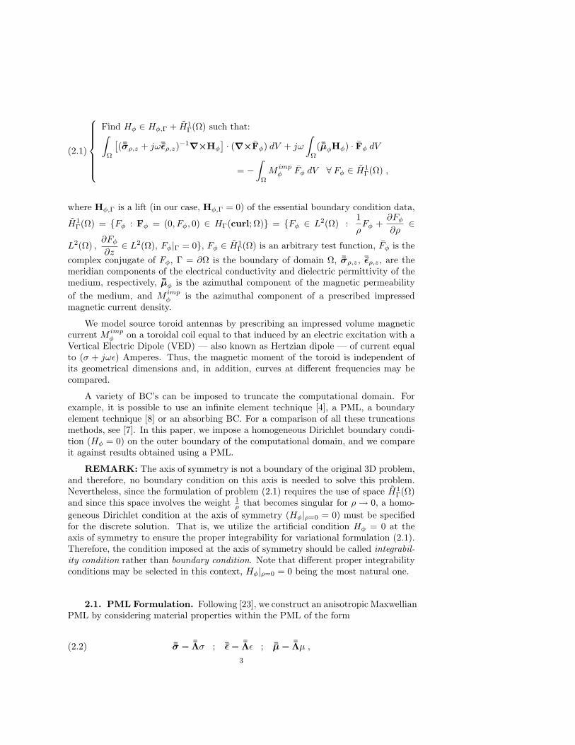
Next, we analyze the computational cost for PMLs combined with our adaptivealgorithm. For each computational domain we study the behavior of the discretiza-tion error (disregarding the modeling error due to the truncation of the computationaldomain) as a function of the problem size (number of unknowns). In Table 4.2 we dis-play the discretization error and the corresponding number of unknowns for differentcomputational domains. Note that these results depend on the initial grid, which isdifferent for each computational domain (although all of them are based on geomet-rically graded grids). Nevertheless, the results of Table 4.2 provide an indication ofthe performance associated with each computational domain and PML. These resultsshow a considerable reduction (about 50%) in terms of the number of unknowns whenintroducing PML 2 as opposed to all other cases displayed in Table 4.2. It is notewor-thy that even with the poorly designed discontinuous PML 3 we obtain results thatare competitive with those of the other cases, since the corresponding solution is alsopiecewise smooth.

Figures 4.4 and 4.5 display the logs2 corresponding to a casing resistivity equalto 10−6Ω ·m and 10−10Ω ·m, respectively. We have computed these logs by utilizing

2A log is a plot displaying the response of the logging instrument as we move it in the verticaldirection along the axis of the borehole.

8

Fig. 4.3. Through-casing resistivity problem. Relative error of the imaginary part of the quan-tity of interest according to Eq. (4.1) as a function of the vertical length of the computational domain.Different curves indicate different resistivities of the casing, ranging from 10−10Ω ·m to 10−6Ω ·m.Results obtained by goal-oriented hp-adaptivity.

two different computational domains, viz. a 10m × 5m domain with PML 2, and a3200m×800m domain without a PML. Fig. 4.4 shows that the computed amplitude issimilar for both computational domains, whereas the phase significantly differs. Thisillustrates that a large computational domain of 3200m × 800m without a PML caninduce considerable phase error. In Fig. 4.5, we obtain similar results when consideringeither of the two computational domains described above.

We observe a large frequency shift of approximately 160 degrees in Fig. 4.5 dueto the presence of a highly conductive casing in a highly resistive formation, as can bephysically expected. In addition, a “horn” in the amplitude appears when comparedto Figure 4.4.

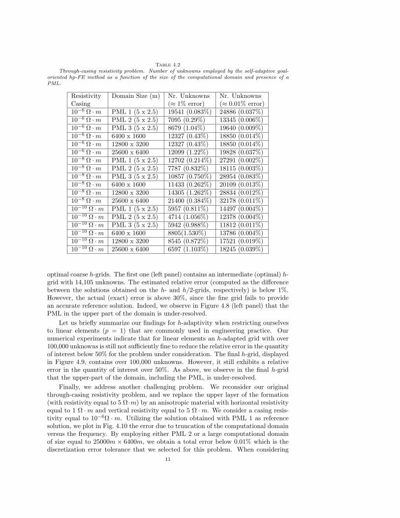
An hp-grid produced by the self-adaptive goal-oriented hp-FE method with PML 2and a casing resistivity equal to 10−6Ω·m is displayed in Figure 4.6 for exemplification.The grid contains 7421 unknowns (of which 80 % are used in the PML), and it deliversa discretization error in the quantity of interest below 0.2%. Large elements of high-order approximation are effective in approximating the smooth part of the solution,while small elements of low order are more suitable for approximating abrupt spatialvariations due to singularities. On the outer part of the casing, we observe morerefinements than on the inner part of the casing, since it is physically known that thequantity of interest exhibits little sensitivity to the conductivity inside the borehole.

To assess the importance of refinements in both h and p, let us consider belowan adaptive goal-oriented FE method with fixed polynomial order of approximation pbut variable mesh size h. To guide optimal refinements for a given coarse h-grid, weutilize the globally h-refined grid, that is, the h/2-grid, where, in two dimensions, all

9

Table 4.1Through-casing resistivity problem. Real and Imaginary parts of the quantity of interest —

given by Eq. (4.1) — as a function of the size of the computational domain and presence of a PML.Results obtained by goal-oriented hp-adaptivity.

Resistivity Domain Size Real Part Imag PartCasing (m) (A/m) (A/m)10−6 Ω ·m PML 1 (5 x 2.5) 1.2320E-6 -8.5928E-910−6 Ω ·m PML 2 (5 x 2.5) 1.2320E-6 -8.5960E-910−6 Ω ·m PML 3 (5 x 2.5) 1.2320E-6 -8.6016E-910−6 Ω ·m 400 x 100 1.3382E-6 -2.0264E-810−6 Ω ·m 1600 x 400 1.2169E-6 -1.2622E-810−6 Ω ·m 6400 x 1600 1.2295E-6 -8.1076E-910−6 Ω ·m 12800 x 3200 1.2320E-6 -8.3840E-910−6 Ω ·m 25600 x 6400 1.2320E-6 -8.5968E-910−8 Ω ·m PML 1 (5 x 2.5) 1.7188E-10 -2.0959E-1110−8 Ω ·m PML 2 (5 x 2.5) 1.7188E-10 -2.0959E-1110−8 Ω ·m PML 3 (5 x 2.5) 1.7188E-10 -2.0957E-1110−8 Ω ·m 400 x 100 1.8772E-10 -1.4463E-1110−8 Ω ·m 1600 x 400 1.7077E-10 -2.3905E-1110−8 Ω ·m 6400 x 1600 1.7124E-10 -1.9548E-1110−8 Ω ·m 12800 x 3200 1.7120E-10 -2.0900E-1110−8 Ω ·m 25600 x 6400 1.7188E-10 -2.0960E-1110−10 Ω ·m PML 1 (5 x 2.5) 1.4255E-13 2.2710E-1510−10 Ω ·m PML 2 (5 x 2.5) 1.4255E-13 2.2710E-1510−10 Ω ·m PML 3 (5 x 2.5) 1.4255E-13 2.2709E-1510−10 Ω ·m 400 x 100 1.4198E-13 2.1780E-1510−10 Ω ·m 1600 x 400 1.4256E-13 2.3695E-1510−10 Ω ·m 6400 x 1600 1.4256E-13 2.2188E-1510−10 Ω ·m 12800 x 3200 1.4255E-13 2.2703E-1510−10 Ω ·m 25600 x 6400 1.4255E-13 2.2710E-15

elements are divided into four element sons. We denote the globally h-refined grid asthe fine grid. Then, we employ an adaptive strategy that is analogous to the one forhp-adaptivity with the only provision that the polynomial order of approximation premains unchanged.

The convergence behavior of the h-adaptive method restricted to polynomial-approximation order p = 2 (quadratic basis functions) and combined with a PML isdisplayed in Figure 4.7, where the discretization error is measured with reference tothe solution that is provided by the hp-adaptive method. The results displayed inFigure 4.7 and their comparison to the results given in Table 4.2 illustrate that the h-adaptive method combined with a PML is less accurate for solving the through-casingresistivity problem under consideration. This observation indicates that in the presentcase, a restriction of the approximation order to p = 2 significantly limits the efficiencyof the method when compared to the hp-adaptive method. In particular, we observethat the sequence of coarse h-grids delivers for 50, 000 unknowns an error that is stilllarger than 10%. Furthermore, for any coarse grid with fewer than 15, 000 unknowns,the fine grid delivers large errors (above 30 %), and therefore, is unable to guideoptimal refinements. To further support this observation, we display in Figure 4.8 two

10

Table 4.2Through-casing resistivity problem. Number of unknowns employed by the self-adaptive goal-

oriented hp-FE method as a function of the size of the computational domain and presence of aPML.

Resistivity Domain Size (m) Nr. Unknowns Nr. UnknownsCasing (≈ 1% error) (≈ 0.01% error)10−6 Ω ·m PML 1 (5 x 2.5) 19541 (0.083%) 24886 (0.037%)10−6 Ω ·m PML 2 (5 x 2.5) 7095 (0.29%) 13345 (0.006%)10−6 Ω ·m PML 3 (5 x 2.5) 8679 (1.04%) 19640 (0.009%)10−6 Ω ·m 6400 x 1600 12327 (0.43%) 18850 (0.014%)10−6 Ω ·m 12800 x 3200 12327 (0.43%) 18850 (0.014%)10−6 Ω ·m 25600 x 6400 12099 (1.22%) 19828 (0.037%)10−8 Ω ·m PML 1 (5 x 2.5) 12702 (0.214%) 27291 (0.002%)10−8 Ω ·m PML 2 (5 x 2.5) 7787 (0.832%) 18115 (0.003%)10−8 Ω ·m PML 3 (5 x 2.5) 10857 (0.750%) 28954 (0.083%)10−8 Ω ·m 6400 x 1600 11433 (0.262%) 20109 (0.013%)10−8 Ω ·m 12800 x 3200 14305 (1.262%) 28834 (0.012%)10−8 Ω ·m 25600 x 6400 21400 (0.384%) 32178 (0.011%)10−10 Ω ·m PML 1 (5 x 2.5) 5957 (0.811%) 14497 (0.004%)10−10 Ω ·m PML 2 (5 x 2.5) 4714 (1.056%) 12378 (0.004%)10−10 Ω ·m PML 3 (5 x 2.5) 5942 (0.988%) 11812 (0.011%)10−10 Ω ·m 6400 x 1600 8805(1.530%) 13786 (0.004%)10−10 Ω ·m 12800 x 3200 8545 (0.872%) 17521 (0.019%)10−10 Ω ·m 25600 x 6400 6597 (1.103%) 18245 (0.039%)

optimal coarse h-grids. The first one (left panel) contains an intermediate (optimal) h-grid with 14,105 unknowns. The estimated relative error (computed as the differencebetween the solutions obtained on the h- and h/2-grids, respectively) is below 1%.However, the actual (exact) error is above 30%, since the fine grid fails to providean accurate reference solution. Indeed, we observe in Figure 4.8 (left panel) that thePML in the upper part of the domain is under-resolved.

Let us briefly summarize our findings for h-adaptivity when restricting ourselvesto linear elements (p = 1) that are commonly used in engineering practice. Ournumerical experiments indicate that for linear elements an h-adapted grid with over100,000 unknowns is still not sufficiently fine to reduce the relative error in the quantityof interest below 50% for the problem under consideration. The final h-grid, displayedin Figure 4.9, contains over 100,000 unknowns. However, it still exhibits a relativeerror in the quantity of interest over 50%. As above, we observe in the final h-gridthat the upper-part of the domain, including the PML, is under-resolved.

Finally, we address another challenging problem. We reconsider our originalthrough-casing resistivity problem, and we replace the upper layer of the formation(with resistivity equal to 5 Ω ·m) by an anisotropic material with horizontal resistivityequal to 1 Ω ·m and vertical resistivity equal to 5 Ω ·m. We consider a casing resis-tivity equal to 10−6Ω ·m. Utilizing the solution obtained with PML 1 as referencesolution, we plot in Fig. 4.10 the error due to truncation of the computational domainversus the frequency. By employing either PML 2 or a large computational domainof size equal to 25000m × 6400m, we obtain a total error below 0.01% which is thediscretization error tolerance that we selected for this problem. When considering

11

Fig. 4.4. Through-casing resistivity problem with a resistivity of casing equal to 10−6Ω · m.Amplitude (left) and phase (right) of the final log. The two curves were obtained on two differentcomputational domains: A 10m× 5m domain with PML 3, and a 3200m× 800m domain without aPML. Results obtained by goal-oriented hp-adaptivity.

Fig. 4.5. Through-casing resistivity problem with a resistivity of casing equal to 10−10Ω · m.Amplitude (left) and phase (right) of the final log. The two curves were obtained on two differentcomputational domains: A 10m× 5m domain with PML 3, and a 3200m× 800m domain without aPML. Results obtained by goal-oriented hp-adaptivity.

smaller domains, we observe the effect of the domain truncation error which may be-12

P M LPML

t←− Transmitter

t←− Receiver It←− Receiver II P

ML

PMLP M L

Fig. 4.6. Through-casing resistivity problem. hp-grid with 7421 unknowns delivered by theself-adaptive goal-oriented hp-FE method. Different colors indicate different polynomials orders ofapproximation, from 1 (light) up to 9 (dark). Size of computational domain: 5m × 2.5m, includinga 0.5m thick PML.

Fig. 4.7. Through-casing resistivity problem with resistivity of casing equal to 10−6Ω · m.Convergence history (number of degrees of freedom — unknowns — of the coarse grid vs. relativeerror of the quantity of interest in percentage) delivered by the self-adaptive goal-oriented h-FEmethod, with p = 2, combined with the PML 2 (5m × 2.5m).

13

P M LPML

t←− Transmitter

t←− Receiver It←− Receiver II P

ML

PMLP M L

P M LPML

t←− Transmitter

t←− Receiver It←− Receiver II P

ML

PMLP M L

Fig. 4.8. Through-casing resistivity problem. Two h-grids (with p = 2) delivered by the self-adaptive goal-oriented h-FE method. Left panel: Intermediate h-grid with 14105 unknowns, deliv-ering an error of over 30%. Right panel: Final h-grid with 76643 unknowns, delivering an error of2%. Size of computational domain: 5m × 2.5m, including a 0.5m thick PML 2.

come as large as 5% for a domain of size 1600m×400m. As a general trend, Fig. 4.10indicates a monotonic decrease of the error with increasing frequency (as physicallyexpected). Note, however, that there are exceptions to this monotonic behavior asevidenced by Fig. 4.10.

14

P M LPML

t←− Transmitter

t←− Receiver It←− Receiver II P

ML

PMLP M L

Fig. 4.9. Through casing resistivity problem. Final h-grid with p = 1, containing 104834unknowns, and delivering an error over 50%. Size of computational domain: 5m× 2.5m, includinga 0.5m thick PML 2.

5. CONCLUSIONS. We have shown that numerical reflections from domaintruncation for a layered medium with high-material constrasts are minimized witha self-adaptive goal-oriented hp-FE method in combination with a PML. Such anadaptive method is capable of delivering optimal grid refinements and, thus, it cansubstantially improve the performance of PMLs.

For problems with material coefficients varying by up to ten orders of magnitudewithin the PML, the self-adaptive goal-oriented hp-FE method automatically con-structs a grid that exhibits minimum reflections (below 0.001% relative error in thequantity of interest for a moderate number of unknowns), even when considering dis-continuous PMLs. Thus, for through-casing resistivity measurements, we can reducethe size of the computational domain from, for instance, 25,000m to 5m by using aPML in combination with our adaptive algorithm. We have demonstrated that thisneither compromises the accuracy of the magnitude nor of the phase of the computedlogging response. Moreover, the number of unknowns that are needed to solve theproblem to a prescribed accuracy can be significantly reduced by using a PML en-hanced with adaptivity instead of a large domain without PML. Thus, we have shownthat PMLs can be successfully employed not only for pure wave propagation problemswith quasi-uniform materials, but also for engineering applications with high materialcontrast within the PML region.

Furthermore, we have shown that a PML combined with a goal-oriented FEmethod that is self-adaptive only in the element size h may be considerably lessaccurate than the corresponding hp-method and require orders of magnitude moreunknowns to achieve the same level of accuracy. This indicates that adaptivity in

15

Fig. 4.10. Anisotropic through-casing resistivity problem with resistivity of casing equal to10−6Ω · m. Relative error of the absolute value of the quantity of interest as a function of thefrequency. Different curves indicate different domain sizes: 400m× 100m, 1600m× 400m, 6400m×1600m, 25600m × 6400m, and 5m × 2.5m (with PML 2). Results obtained by goal-oriented hp-adaptivity.

both element size h and polynomial approximation order p is essential for the accu-racy of the solution.

Finally, we have demonstrated that PMLs combined with the self-adaptive goal-oriented hp-FE method maintain good performance in the presence of anisotropicmaterials, as well as at different frequencies.

ACKNOWLEDGMENTS. This work was financially supported by Baker At-las and The University of Texas at Austin’s Joint Industry Research Consortium onFormation Evaluation sponsored by Aramco, Baker Atlas, BP, British Gas, Chevron,ConocoPhillips, ENI E&P, ExxonMobil, Halliburton, Marathon, Mexican Institutefor Petroleum, Hydro, Occidental Petroleum, Petrobras, Schlumberger, Shell E&P,Statoil, TOTAL, and Weatherford International Ltd. Moreover, the fourth authorwas supported by the Netherlands Organization for Scientific Research (NWO) andthe ICES Postdoctoral Fellowship Program of the Institute for Computational Engi-neering and Sciences (ICES) at The University of Texas at Austin. This support isgratefully acknowledged.

16

REFERENCES

[1] I. Babuska and B.Q. Guo, Approximation properties of the h-p version of the finite elementmethod., Computer Methods in Applied Mechanics and Engineering, 133 (1996), pp. 319–346.

[2] I. Babuska and B. Q. Guo, Regularity of the solution of elliptic problems with piecewiseanalytic data. I. Boundary value problems for linear elliptic equations of second order,SIAM J. Math. Anal., 19 (1988), pp. 172–203.

[3] J. Berenger, A perfectly matched layer for the absortion of electromagnetic waves., J. Comput.Phys., 114 (1994), pp. 185–200.

[4] W. Cecot, W. Rachowicz, and L. Demkowicz, An hp-adaptive finite element method forelectromagnetics. III: A three-dimensional infinite element for Maxwell’s equations., In-ternational Journal of Numerical Methods in Engineering, 57 (2003), pp. 899–921.

[5] W. C. Chew and W. H. Weedon, A 3D perfectly matched medium from modified Maxwell’sequations with streched coordinates., Microwave Opt. Tech. Lett., 7 (1994), pp. 599–604.

[6] L. Demkowicz, Computing with hp-Adaptive Finite Elements. Volume I: One and Two Di-mensional Elliptic and Maxwell Problems., Chapman and Hall, 2006.

[7] I. Gomez-Revuelto, L.E. Garcia-Castillo, and L.F. Demkowicz, A comparison betweenseveral mesh truncation methods for hp-adaptivity in electromagnetics, in (ICEAA07),Torino (Italia), Sept. 2007. Invited paper to the Special Session “Numerical Methods forSolving Maxwell Equations in the Frequency Domain”.

[8] I. Gomez-Revuelto, L. E. Garcia-Castillo, D. Pardo, and L. Demkowicz, A two-dimensional self-adaptive hp finite element method for the analysis of open region problemsin electromagnetics, IEEE Transactions on Magnetics, 43 (2007), pp. 1337–1340.

[9] A. A. Kaufman, The electrical field in a borehole with casing., Geophysics, 55 (1990), pp. 29–38.

[10] C. Michler, L. Demkowicz, J. Kurtz, and D. Pardo, Improving the performance of per-fectly matched layers by means of hp-adaptivity, Numerical Methods for Partial DifferentialEquations, 23 (2007), pp. 832–858.

[11] D. Pardo, L. Demkowicz, C. Torres-Verdin, and M. Paszynski, Simulation of resistivitylogging-while-drilling (LWD) measurements using a self-adaptive goal-oriented hp-finiteelement method., SIAM Journal in Applied Mathematics, 66 (2006), pp. 2085–2106.

[12] , A goal oriented hp-adaptive finite element strategy with electromagnetic applications.Part II: electrodynamics., Computer Methods in Applied Mechanics and Engineering., 196(2007), pp. 3585–3597.

[13] D. Pardo, L. Demkowicz, C. Torres-Verdin, and L. Tabarovsky, A goal-oriented hp-adaptive finite element method with electromagnetic applications. Part I: electrostatics.,International Journal for Numerical Methods in Engineering, 65 (2006), pp. 1269–1309.

[14] D. Pardo, C. Torres-Verdin, and L. Demkowicz, Simulation of multi-frequency boreholeresistivity measurements through metal casing using a goal-oriented hp-finite elementmethod., IEEE Transactions on Geosciences and Remote Sensing, 44 (2006), pp. 2125–2135.

[15] , Feasibility Study for Two-Dimensional Frequency Dependent Electromagnetic SensingThrough Casing., Geophysics, 72 (2007), pp. F111–F118.

[16] M. Paszynski, L. Demkowicz, and D. Pardo, Verification of goal-oriented hp-adaptivity.,Computers and Mathematics with Applications, 50 (2005), pp. 1395–1404.

[17] S. Prudhomme and J. T. Oden, On goal-oriented error estimation for elliptic problems: ap-plication to the control of pointwise errors., Computer Methods in Applied Mechanics andEngineering, 176 (1999), pp. 313–331.

[18] C. J. Schenkel and H. F. Morrison, Electrical resistivity measurement through metal casing.,Geophysics, 59 (1994), pp. 1072–1082.

[19] Ch. Schwab, p- and hp-finite element methods, Numerical Mathematics and Scientific Com-putation, The Clarendon Press Oxford University Press, New York, 1998. Theory andapplications in solid and fluid mechanics.

[20] B. Stupfel, A Study of the Condition Number of Various Finite Element Matrices Involvedin the Numerical Solution of Maxwell’s Equations, IEEE Transactions on Antennas andPropagation, 52 (2004), pp. 3048–3059.

[21] F.L. Teixeira and W.C. Chew, Fast and efficient algorithms in computational electromagnet-ics: advances in the theory of perfectly matched layers (pp. 283-346), Eds.: W.C. Chew,J.M. Jin, E. Michielsen, J. M. Song, 2001.

[22] F. L. Teixeira and W. C. Chew, PML-FDTD in cylindrical and spherical grid., IEEE Mi-crowave Guided Wave Lett., 7 (1997), pp. 285–287.

17

[23] , Systematic derivation of anisotropic PML absorbing media in cylindrical and sphericalcoordinates., IEEE Microwave Guided Wave Lett., 7 (1997), pp. 371–373.

[24] W.B. Vail, S.T. Momii, R. Woodhouse, M. Alberty, R.C.A. Peveraro, and J.D. Klein,Formation resistivity measurements through metal casing., SPWLA 34th Annual LoggingSymposium, F (1993).

[25] D. H. Werner and R. Mittra, Frontiers in electromagnetics: A systematic study of perfectlymatched absorbers, pp. 609-642), John Wiley and Sons Inc., 2000.

[26] X. Wu and T. M. Habashy, Influence of steel casings on electromagnetic signals., Geophysics,59 (1994), pp. 378–390.

18