An operational test for distinguishing between complicated and chaotic behavior in deterministic systems
M. Johnson *, J. Habyarimana Department of Mechanical Engineering, Massachusetts Institute of Technology, Room 3-264, 77 Massachusetts Ave., Cambridge,
MA 01139, USA Received 29 April 1997; received in revised form 5 December 1997; accepted 15 January 1998
in a tube without diffusion) show a different charac- ter with cr 2 varying as t 2 (or N 2 for a discrete process
where N is the number of steps). 1
We here use a similar scheme to investigate chaotic
mappings. We consider a general mapping such that
-~N+I = g(~CN), (2)
where . ~ n . We introduce an added direction y such
that [:~, y]E• n+l and we define a mapping such that
YN+I = YN -b f(.XN). (3)
! Actually, Taylor found that Eq. (1) is only valid for t >> O.07a2/D as this is the average time necessary for a tracer particle to sample all locations in the cross-section; for shorter times, convective effects dominate and o -2 grows a s t 2. A related constraint is that the cross-section must be bounded; we will later examine the consequence of a process whose cross-section is unbounded.
M. Johnson, J. Habyarimana/Physica D 116 (1998) 289-300
Table 1 form of a 2 for different Anticipated systems
Nature of system to be investigated Example as N ----> oo,
)~N+I = g(-~N)
Behavior of a~, as N + vc
YN+I = YN qf f ( f ;N)
291
Single attractive fixed point Single attractive limit cycle
Multiple fixed points
Multiple attractive limit cycles
Topologically transitive but without
mixing (non-chaotic)
Chaotic
Logistic equation with 2. < 3 Logistic equation with )~ > 3 and )~ < 3.57
Twisting map for rational values of
Twisting map for irrational values of ot
Trigonometric map
Bounded Bounded
N 2 a 7, grows as N 2 a 2 grows as
~ N 2 cr~ grows as
N ~, ~ 2. a 7, grows as ot
= 1: diffusive; ot # 1,0 < ~ < 2: anomalous diffusion; t~ > 2: diffusive in unbounded domain
In this table, f is assumed to be a bounded function that is not uniform throught the domain of ~. As noted in the text, it is possible in cases where cr~ is expected to grow as c* N c~ that the constant c is zero: in those cases, the behavior is non-determinant
and another function f is chosen.
The coordinate y is analogous to the streamwise di-
rection in the Taylor dispersion problem. Note that
displacements in the y-direction depend only on the
particle location, .~, as determined by the original pro-
cess being investigated. Thus, no additional dynamics
are added to the process by the function f .
In the Taylor dispersion problem, the function 3" is
the axial velocity normal to the cross-sectional plane.
In that problem, the function f is restricted to be
time-independent, or at least statistically steady (for
turbulent flows) [15]; it is also required that the axial
flow not be uniform within the domain of interest. Oth-
erwise, diffusive behavior in the axial diraction will
not be seen.
For chaotic processes, no theoretical analysis is
available to indicate the requirement for the function
f . This would be a useful topic for further research
in this area. We have found that, in practice, most
choices for f are acceptable. The only restriction is a
practical one that the function chosen must generate
dispersion in the y-direction that increases with the
step number N, and this is a straightforward propo-
sition to determine. In practice, we allow f to be a
linear function of .~ and measure the rate of change
of the variance in the y-direction. If the variance
does not grow with N, another function f is chosen.
We have found that a linear function almost always
suffices, but we will show one example in which a
linear function does not generate an increasing disper-
sion; for that case, we then allow f to be quadratic.
We do not investigate, in this paper, the theoretical
requirements for the function f .
We introduce tracer particles (dispersed randomly
throughout the domain ~") that are then transported by
the process defined by Eqs. (2) and (3). By monitoring
the growth of the variance of the tracer distribution
in the y-direction, a~ (an ensemble average), we can
evaluate if the process is a diffusive one. Specifically,
a process that is diffusive will have the variance of
the tracer distribution grow as N ~'. c~ -¢ 2, while a
non-diffusive process will have its variance grow as
N2[16]. The most generic case of a diffusive process
will have o~ = 1 ; diffusive cases with c~ < 2 and ot -¢
1 are referred to as exhibiting "anomalous diffusion".
The anticipated form of a 2 for different systems is
shown in Table 1. We will find that some processes will show no
long-term in a~., which is a non-determinant case that
may or may not be random (chaotic). This happens
relatively frequently for non-chaotic mappings as a consequence of the simple form of the attractors that
typically arise in one-dimensional systems which lead
to all particles approaching a single attractor (fixed
point or limit cycle), and thus cr~ remains bounded.
292 M. Johnson, 3". Habyarimana/Physica D 116 (1998) 289-300
In such a case, all functions f (Eq. (3)) will lead to
an upperbound for cr 2. Chaotic processes occasionally
(rarely in our experience) can exhibit bounded values
of a 2 for a particular f , but will show a 2 to grow with
N for most other choices for f . A single case is de-
scribed (the "biological" map described below) where
a linear function f leads to bounded values of ~2 but
a quadratic function shows cr 2 to grow with N.
It is also possible to have a "mixed regime" for near
integrable systems in which part of the domain is reg-
ular and the remainder is chaotic [16]. Although we
do not further consider such processes here, they can
be handled by using similar methods to those we de-
scribe, but particles must be seeded exclusively in the
chaotic domain to see diffusive growth of the variance.
The ensemble-averaged quantities characterizing
the process dynamics were computed only after the
stable attractor (fixed point, limit cycle or strange
attractor) was reached. The particles were initially
distributed randomly and uniformly throughout the
domain (usually with 0 < x0 < 1). Double-precision
was used for all calculations. We began our computa-
tions of the parameters for N > 1000. The effective
diffusion coefficient was calculated as
cr2(1000 + N) - or2(1000) Deft = lim ~ ~ (4)
N--~ 2N
We compared use of the diffusive criterion for chaos
with the two other criteria, namely a positive Lyapunov
exponent and the autocorrelation coefficient dropping
to zero. The Lyapunov exponent was computed by
introduction a small perturbation (e = 10 -9) to the
system state at N = 1000 and then computing the
exponent/~ as
1 12 = ~ { l n IxIloOO+N - - XlOOO+N[) / ,~ , (5)
where { } is an ensemble average and XII000+N is the value of x at step 1000 + N having been perturbed at step 1000 by e.
where Crx (m) is the standerd deviation of the distribu-
tion of x at step m. Note that if r should ever return
to 1 for any N > 0, the process cannot be chaotic.
3. The logistic equation
We first consider the well-known logistic equation:
XN+I = )~XN(I -- XN) . (7)
This equation exhibits chaotic behavior when the pa-
rameter Z is greater than approximately 3.57 [17]
We introduce motion in the added direction y with
f ( X N ) = XN -- 0.5:
YN+I = YN -1- (XN -- 0.5), (8)
and then compute the Layapunov exponent, the auto-
correlation coefficient and the variance.
For ~. < 3 (attractive fixed points), in all cases,
the Layapunov exponent is found to be negative, and
the correlation coefficient remains at I; cr~ remained
constant since all particles are attracted to the single
stable fixed point. Similar behavior is seen for 3 <
~. < 3.57 (attractive orbits), although there is a long
time oscillatory behavior of the variance. An example
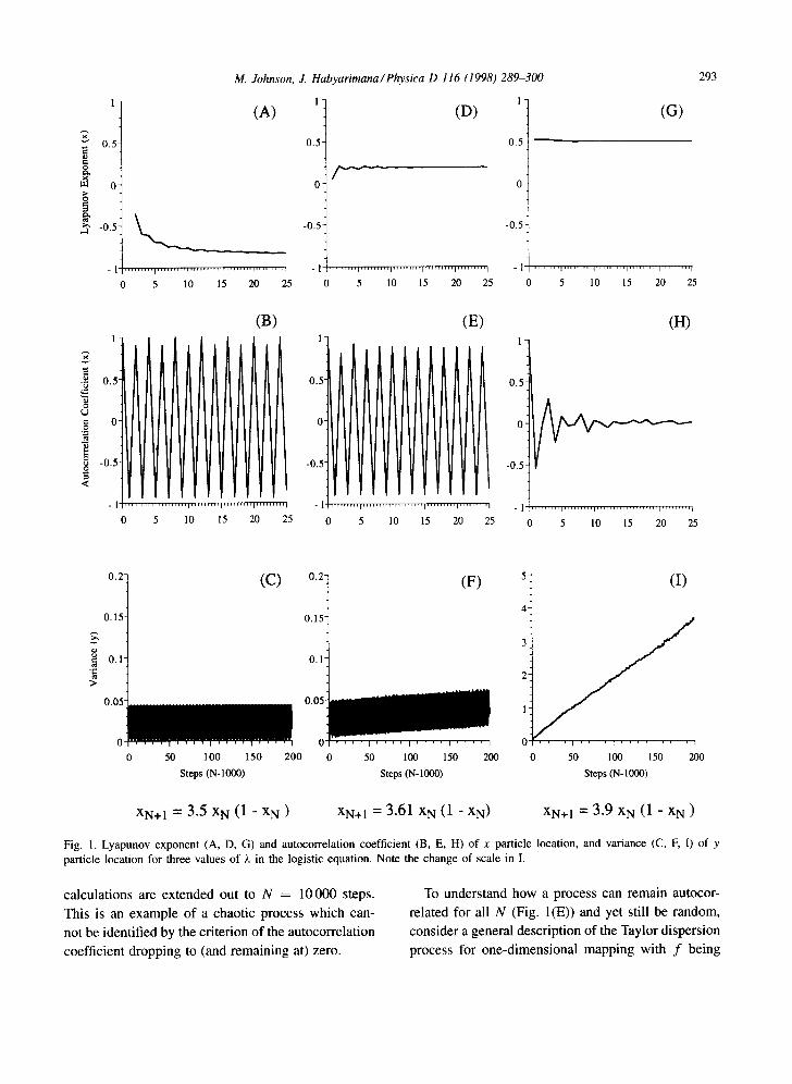
is shown in Figs. I (A-C) for ~. = 3.5. As expected, no
growth was seen in the variance once the limit cycle
was reached, even if the computation was extended
to 10 000 steps. Similar behavior was seen if different
functions f were chosen (e.g. f ( X N ) = X 2 ) .
For ~. > 3.57, the onset of chaos is accompanied by
a positive Layapunov exponent, a decreasing correla-
tion coefficient and the variance growing with N in a
fashion consistent with diffusive transport (a~ ~ N).
Figs. I (G-I) show the behavior of the three chaotic
measures for ~. = 3.9; all three measure are consistent
with a chaotic process with a positive Lyapunov expo-
nent, the autocorrelation coefficient dropping to zero
and the variance in the y-direction growing linearly
with N. However, for ~ = 3.61, a parameter value
also recognized to be the chaotic regime, while both
the Lyapunov exponent and the growth of the vari-
ance in the y-direction are consistent with a chaotic process (Figs. I(D) and (F)), the autocorrelation co- efficient does not drop to zero (Fig. I(E)) even if the
0.5 -fi
m O g
~ -0.5-
0 5 10 15 20 25
M. Johnson, J. Habyarimana/Physica D 116 (1998) 289-300
1- I - (A) " (D) "
0.5 0.5-
-0.5
- I . . . . . . . . . I . . . . . . . . . I " ' " ' " ' 1 . . . . . . . . . I . . . . . . . . . I
0 5 10 15 20 25
-0.5
(G)
' " . . . . . . I ' " ' . . . . . I . . . . . . . . . I " " . . . . . I " . . . . . . . I
XN+ 1 = 3 . 5 X N (1 - x N ) XN+ l = 3 . 6 1 X N (1 - XN) XN+ l = 3 . 9 X N (1 - X N )
Fig. 1. Lyapunov exponent (A, D, G) and autocorrelation coefficient (B, E, H) of x particle location, and variance (C, F, I) of y particle location for three values of k in the logistic equation. Note the change of scale in I.
calculations are extended out to N = 10000 steps.
This is an example of a chaotic process which can-
not be identified by the criterion of the autocorrelation
coefficient dropping to (and remaining at) zero.
To understand how a process can remain autocor-
related for all N (Fig. I(E)) and yet still be random,
consider a general description of the Taylor dispersion
process for one-dimensional mapping with f being
294 M. Johnson, J. Habyarimana/Physica D 116 (1998) 289-300
chosen to be linear. Letting XN+ 1 : g(xN) and
YN+I ---- YN + (XN -- a), we then find that
N I N - I
~ 2 ( U ) = Z Z ((xi - (xi))(xj -(xj))) i=0 .i=o
N I N - I
= Z Z rx(i, j)~x(i)~z~(j), (9) i = 0 j = 0
where rx(i, j ) is the correlation coefficient between
the particle's x location at step i and step j , and a2(i)
is the variance of the particle's x location at step i.
(Jones and Young [16] find an analogous expression
for a continuous process but use an autocorrelation
function that is not normalized.) 2 Note here that the particularly simple form for a),
results because of the simple form used for f(XN), i.e. linear. We can then identify those process in which
~ff ~ N (i.e. diffusive processes) and we find a number
of conditions under which this can occur: (i) rx (i, i +
k) = 0 for all k > n (this occurs for the logistic
equation for ~. = 4 with n = 1), (ii) rx(i, i + k) e k, (iii) r x ( i , i + k ) ~ k -~ withot > 1 (for 0 <
_< 1, anomalous dispersion [16] results), and (iv) a
summation condition on the correlation coefficient:
N k ) lim Z rx(i,i + k)crx(i)~x(i + < S, (10)
N --~ ~x~ k=0
where S is some positive constant. As ~ ( i ) usually
approaches a constant value for large N (i.e. ~ be-
comes roughly 1/2 the domain size), this criterion is
equivalent to a requirement that the sum over N (or
temporal integral) of the autocorrelation coefficient
approaches a constant value for large N. This can be
achieved either by the autocorrelation coefficient ap-
proaching 0 for large N, or by a long time oscillation,
as seen in the case for ~. = 3.61 (Fig. I(E)). Thus we
see that the diffusive criterion for chaos is somewhat less strict than a requirement that the autocorrelation coefficient drops to zero for large N.
4. Other well-known mappings
We next considered a number of common mappings including:
(a) the twisting map [1,18]
ON+ 1 = O N + 2 7 r a , (1 l)
(b) a trigonometric map [6,19]
xu+l = 0.999 sin(Jrxu), (12)
(c) an exponential or "biological" map [6,20]
Xu+l = Xu exp[3(I -- XN)], (13)
(d) the x values of the H6non map [6,21]
XU+l = S.N ~- I - - 1.4x~v, ZN+I = 0.3XN. (14)
The first of these mappings is not chaotic while the
other three are.
For rational values of~ , the twisting mapping has an
infinite number of periodic points; for irrational values
of ~, there are no periodic points. However in neither
case is the process topologically transitive (there is no
mixing). Thus, this is not a chaotic process.
The particles were seeded initially uniformly be-
tween 0 and 2re. The Lyapunov exponent was found to
be zero for all values of ~. For ~ rational, the correla-
tion coefficient always returned one (periodic orbits);
for o~ irrational, the correlation coefficient returned ar-
bitrarily close to one. We chose f (Ou) = ON (linear),
substituted into Eq. (3) and used Eq. (11) to find the
behavior of c~. We found that for both rational and
irrational values of a, a2 varied with N 2, as expected
for a non-random process. For ot rational, this growth
occurred from one period to the next, while for a ir-
rational, this growth was considerably slower and oc-
curred in an quasi-oscillatory fashion. Thus, all three
tively, h(N) = 2 N has already been shown to chaotic
[1]. h(N) = N + 1 can be shown to be chaotic by
recognizing that (i) the mapping is sensitive to initial
conditions (by design), and (ii) it has a dense set of
periodic points. Therefore, given that any two of De-
vaney's three conditions represent a sufficient condi-
tion for chaos [2-4], this system is chaotic, h(N) =
N 2 4- 1 can be shown to be chaotic in a similar fash-
ion, although, in this case, it is easier to demonstrate
296 M. Johnson, .I. H a b y a r i m a n a / P h y s i c a D 116 (1998) 2 8 9 - 3 0 0
that the system is topologically transitive rather than
showing it to have dense periodic points.
We proceeded to investigate how the three differ-
ent indicators of chaos we have used behave for these
three mappings. Using Eq. (8) to characterize trans-
port in the linked coordinate, we found that using
Eq. (15) with h(N) = 2 N gave an agreement between
all three indicators of chaos. This was, of course, ex-
pected since we previously investigated the logistic
equation as described in Section 3.
However, a different result was obtained using
h(N) = N + I and N 2 + 1. Clearly, neither of these
functions will give a positive Lyapunov exponent
when substituted into Eq. (15), and our numerical
results confirmed this. Yet measurement of the cor-
relation coefficient and the growth of the variance in
the linked coordinate (using Eq. (8) to characterize
transport in this direction) showed both processes to
be chaotic, in agreement with Devaney's definition.
This was especially surprising for h(N) = N + 1 as
the growth of the error is only linear. (It should be
noted that this latter case is particularly interesting
in that for an initial condition of uniform probability
between x = 0 and x = 1, this process exhibits a 2 very unusual form of anomalous diffusion with %
growing only as In(N).)
Thus, we here have demonstrated that chaotic pro-
cesses do not necessarily have a positive Lyapunov
exponent. The diffusive measure of chaos seems to be
a more robust determinant.
mapping traps the orbits between values of -0 .5 and
0.5; above this value of #, the system exhibits diffu-
sion in the x-direction with a typical Gaussian distri-
bution. We hypothesized that the only reason diffusion
was not observed below this critical value of ~t was that
the orbits were trapped to x values between - 1/2 and
1/2, but that the motions were still diffusive. Thus, we
introduced f ( xN) ---- XN and used Eqs. (3) and (16) to
investigate whether diffusive motion was occurring.
For this case, a different behavior is expected in
terms of the growth of the variance with increasing 2 N. For 0.57 < /z < 0.732644, linear growth of %
with N is expected; however, for/z > 0.732644, the
orbits in the x-direction are not bounded. The Tay-
lor dispersion process shows linear growth of cr 2 with
N only when the orbits in the original domain (R n)
are bounded. However, it has been shown [23] that
for Taylor dispersion in an unbounded shear flow with
constant velocity gradient dVy/dx, the effective diffu-
sion coefficient (Dell) can be related to the molecular
diffusion coefficient (D) as
Deff/D = (dVv/dx)2t 2. (17)
2 grows with t 3 and Def t Note that in this case, %,
grows with t 2 rather than reaching an asymptotic value 2 (a convective, non-chaotic process would show ~ry
growing with t 2 whether or not the cross-section was
bounded). For YN+I = YN +XN, the time step is unity
as is the velocity gradient, and thus this relationship
becomes
6. Diffusion
We next examined a chaotic process that has already
been shown to be positive:
X N + 1 = X N - - [A sin(2rrXN). (16)
This process shows the normal period doubling route
to chaos, with an accumulation point occurring at ap-
proximately # > 0.57. Geisel [10] and Geisel and
Nierwetberg [22] showed a change in character in the
process when # > 0.732644. For /z less than this value, the system is still chaotic, but does not ex-
hibit diffusional behavior in the x-direction, since the
Deff/Dchaos = N 2, (18)
where Dchaos is the diffusion coefficient inherent in the
chaotic process as previously determined by Geisel.
As expected, we found that diffusive motion
(variance growing linearly with N in the linked coor- rdinate y) began for values o f # > 0.57, which the cor-
relation coefficient and Lyapunov exponent confirmed
as the value at which chaos began. This supported
our hypothesis that diffusive motion was apparent for
all chaotic values of/z. We further investigated this phenomenon by examining the relationship between
the diffusion coefficient Dchaos measured in the x- direction (Dchaos = 1/2dcr2x/dx) and the value of
0.1
o
0 O 0 O
M. Johnson, J. Habyarimana / Physica D 116 (1998) 289-300
0.1
o
. . . . I . . . . I ' '
0 . 7 0 . 8
0.01
0 .001
• 0 .0001 o
1 0 ,5 e
0 . 0 1 . . . . i , - 7 ~ - ' ' ' i
0 . 5 0 . 6 0 . 9 1
/1
Fig. 3. Diffusion coefficient as a function of # for X N + I : X N --Id sin(2zrXN). Open circles show values calculated using Taylor dispersion in y-direction; filled circles are calcu- lated directly from growth of second moment in x-direction. The vertical dashed line is at /~ = 0.732644. No filled circles are given for # < 0.732644, since, as explained in the text. the orbits are trapped below this value of # and thus direct calcula- tion of the diffusion in the x-direction cannot be accomplished.
Dchao s determined from Eqs. (4) and (18). As shown
in Fig. 3, an excellent agreement was seen between
the two methods of calculation for/1 > 0.732644.
For 0.57 < # < 0.732644, as mentioned previ-
ously, no direct measure of the diffusion coefficient
(Dchaos) was possible. However, we used the analyti-
cal result for Taylor dispersion in a Couette flow (see
Eq. (20), below, with Dchao s in place of Dintrinsic) to es- timate values of Dchaos, as the orbits were constrained
in this case to be between - 1 / 2 and 1/2. This proce-
dure yielded values of similar order of magnitude to
those found for/~ > 0.732644.
7. Effect o f adde d intr ins ic d i f fus ion
For the chaotic processes investigated, we have
computed the values of the effective diffusion coeffi-
cient (Deft) in the linked coordinate v (Eq. (4)). The
question arises as to whether the magnitude of this
quantity gives additional information concerning the
nature of the chaotic processes being investigated. In particular, does greater chaotic mixing lead to a
greater or less values of Deft? Eq. (1) would suggest the latter, but it must be recalled that Deft" depends not
O O
[0 -6 - o
!
10 ,7 2 o
i
10-si . . . . i 3.5 3.6
%
o o o o
o o
297
o o
°oo o~
o o o
, , , , i ' ' ' i ' ' i , [ , , , , i
3.7 3.8 3 .9 4
k
Fig. 4. Effect ive d i f fus ion coeff ic ient in the l inked coo rd ina t e
v as a func t ion o f ~. as de t e rmined us ing Eqs. (4). (7) and (8).
only on the level of cross-sectional mixing, but also
on the area over which this mixing occurs. As the area
(measured in the appropriate fractal dimension) of
the strange attractor will change for different chaotic
conditions, it is not clear how Dell is quantitatively re-
lated to the extent of the chaotic mixing. An example
is given in Fig. 4 showing the effect of increasing k on
Deft for Eqs. (7) and (8) as determined in Section 3.
To further investigate this, we added intrinsic dif-
fusion, or "noise", to Eq. (7) following the method of
Crutchfield and Farmer [17], and determined the ef-
fect of the intrinsic diffusivity on Deft'. We added the
random variable s to Eq. (7) to yield
X N + I = ~-A'N(1 - - X N ) J - S. ( 1 9 )
s was chosen using a random number generator with
a standard deviation cr 2 * and mean. • = 2 Ointrinsic z e r o
If, due to s, Eq. (19) yielded a value that was outside
of the domain 0 < Xu+l _< l, the value was reflected
back into the domain.
Fig. 5 shows results for Deff as a function of
Dintrinsic for k = 4 and k = 3.61. Also shown is the classical Taylor dispersion result which is found when
X N + 1 = X x -~-S (only intrinsic diffusion, no chaotic
motion). In the latter case, the Taylor dispersion result
(Couette flow) is found to be
'~ 2 2a- Vma x (20)
Deft - 15 Dintrinsic '
298
1
0.1 o
0.01
g~
0.001
0.000l
10 -5 I lO-lO
M. Johnson, J. Habyarimana/Physica D 116 (1998)289-300
8. Discussion and conclusions
\
O • \
I
1
~.=4
0 0 0 0 0 0 0
• ~ . = 3 . 6 1
I I I I I I I
10 .8 10 .6 0.0001 0.01
D intrinsic
Fig. 5. Def t for Eq. (19) as a function of Dintrinsic for £ = 3.61 (squares), £ = 4 (circles), and for Eq. (20) (dashed line).
with 2*a the domain size and Vmax the maximum ax-
ial velocity in the domain. For the given conditions
(Vmax = 1/2; a = 1/2), Deft = 0.00833/Dintrinsic. While the results for £ = 4 show that increas-
ing Dintrinsic leads to a decrease in Deft, as might be anticipated from Eq. (1), £ = 3.61 shows a different
behavior; here the converse occurs. (Note that both
values of ~. approach the classical Taylor result for
high values of Dintrinsic, as one would expected). The different behavior o f £ = 4 and ~. = 3.61 is due to the
change in character of the strange attractor as Dintrinsic
is increased.
While £ = 4 is associated with strange attractor that
spans the entire domain 0 < XN < 1, £ = 3.61 has a
much smaller attractor that is concentrated in two re-
gions (roughly 0.31 < XN < 0.62 and 0.78 < XN <
0.91). Thus, when intrinsic diffusion is added to the
latter case, it increases not only the random mixing
on the strange attractor, but also expands its size, ulti-
mately, for high values of Dintrinsic, filling the domain, 0 < XN < 1. This, of course, affects the magnitude
o f Deft and shows the difficulty of characterizing the
extent of chaotic mixing using Deft, since it charac-
terizes both the extent of mixing and the region over
which mixing occurs. Thus, while we have found Deft to be a useful tool for determining whether or not a given process is chaotic, we cannot yet assign physi- cal significance to its magnitude.
Deterministic processes that exhibit stochastic be-
havior are characterized as "chaotic" if they have a
low number of degrees of freedom and "random"
if they have a high number of degrees of freedom
[6]. This characterization is not well-defined since
there is no sharp boundary between these behaviors.
However, the hallmark and surprising characteristic
of all these deterministic processes is their intrinsic
stochastic behavior. Since stochastic behavior is in-
variably associated with diffusion, we have devised a
test that allows any system to be probed for diffusive
character.
Our new operational test for chaos appears consis-
tent with the definition of chaotic processes, at least
for discrete mappings. Although this test does not
distinguish between low-order and high-order chaotic
systems, other tests already exist to examine that dis-
tinction [6]. While we have examined discrete mapp-
pings, other investigators have used an analogous
scheme to ours for investigating continuous systems
[16,24,25]. These have been flow processes in which
chaotic behavior in the cross-sectional plane has been
demonstrated to lead to diffusive or anomalous diffu-
sive behavior in the axial direction, adding support to
the content that all chaotic processes exhibit diffusive
behavior. However, we have not yet demonstrated
theoretically that Devaney's definition of chaos [1],
in fact, requires diffusive behavior.
We have further shown that two other frequently
used criteria for chaos, a positive Lyapunov exponent
and an autocorrelation coefficient dropping to and re-
maining at zero, fail to be satisfied for some map-
pings that meet Devaney's definition of chaos. In the
case of positive Lyapunov exponent, its requirement
for exponential growth appears to be too strong. De-
vaney's definition only requires sensitivity to initial conditions. As regards the autocorrelation coefficient,
we have shown that diffusive growth of the variance in
the added direction can be related to the autocorrela-
tion coefficient (Eq. (10)). This relationship indicates
that diffusive behavior is associated with the sum (or integral) of the autocorrelation coefficient rather than its value at any single step.
M. Johnson, J. Habyarimana/Physica D 116 (1998) 289-300 299
In summary, we have presented a new technique
for detecting the stochastic behavior characteristic of
chaotic process. In all the cases examined, the tech-
nique has correctly identified chaotic behavior. Further
theoretical studies are necessary to find if Devaney 's
definit ion of chaos necessarily implies stochastic be-
havior.
and thus the variance in this direction cannot cont inue
to grow without bound. This l imitat ion arises because
of a similarity between the functional form of f and
the solution of the difference equation (A. 1). However,
if f is chosen as quadratic, the step leading to Eq. (A.3)
is not possible, and this l imitation in orbit does not
occur.
Acknowledgements
We thank the MIT Undergraduate Research Oppor-
tunities Program for providing support for this project.
We also thank Professors Anthony Patera, Roger
K a m m and Zaichun Feng for helpful discussions.
Appendix A
As ment ioned in Section 4, use of a l inear function
for f ( x N ) in Eq. (3) combined with the exponential
map (13) leads to no long-term growth for a~. We
here demonstrate why that particular result arises. Be-
g inn ing with Eq. (13), we can solve this difference
equation to find that
U
XN+ 1 = X 0 --I 1 e3(l_xi) (A.1)
i=0
Eqs. (3) and (A. 1) can be combined to find the motion
in the added direction y, as
U j - I N
YN+I : ~-~ X.j : ~ X 0 H e3(l-xi) (A.2)
j : 0 j : 0 i =0
or
N
E 3(,-,i/ YN+I = XO e = j : 0
N 3(/ v i) = x0 2..., e . • (A.3)
j=0
Now introducing ZN =--- YN - - N - - l n x0, we find that
ZN+~ -- ZN = e -3z" -- 1. (A.4)
Note that Eq. (A.4) indicates that growth of orbits in
the y-direct ion are limited around the mean position,
References
[ I ] Devaney, An Introduction to Chaotic Dynamical Systems, Addison-Wesley, Reading, MA, 1989.
[2] E. Glasner, B. West, Sensitive dependence on initial conditions, Nonlinearity 6 (1993) 1067-1075.
[3] J. Banks, J. Brooks, G. Cairns, G. Davies, E Stacey, On Devaney's definition of chaos, Amer. Math. Month. 99 (1992) 332-334.
[4] S. Silverman, On maps with dense orbits and the definition of chaos, Rocky Mountain J. Math. 22 (1992) 353-375•
[5] T.-Y. Li. J.A. Yorke, Period three implies chaos. Amer. Math. Month. 82 (1975) 985-992.
[6] W. Marzocchi, Detecting low-dimensional chaos in time series of finite length generated from discrete parameter processes, Physica D 90 (1996) 31-39.
[7] M. Toda, R. Kubo, N. Sait6, Statistical Physics I, Equilibrium Statistical Mechanics, Springer. Berlin, 1983, pp. 206-208.
[8] A. Wolf. J.B. Swift, H.L. Swinney, J.A. Vasatano, Determining Lyapunov exponents from a time series, Physica D 16 (1985) 285-317.
[9] S. Grossman, S. Thomae, Invariant distributions and stationary correlation function of one-dimensional discrete processes, Zeit Naturforschung, A 32 (1977) 1353-1363.
[10] T. Geisel, Deterministic diffusion - a quality of chaos, in: M.G. Velarde (Eds.), Nonequilibrium Cooperative Phenomenon and Related Fields, Plenum Press, New York, 1983, pp. 437-453.
l[ l] A.J. Lichtenberg, M.A. Lieberman, in: Regular and Stochastic Motion, Chapter 5, Springer, New York, 1983.
[12] A.N. Yannacopoulos, G. Rowlands, Calculation of diffusion coefficients for chaotic maps, Physica D 65 (1993) 71-85.
[13] B. Andersson. T. Berglin, Dispersion in laminar flow through a circular tube, Proc. Roy. Soc. London. A 377 ( 1981 ) 251-268.
[14] G.I. Taylor, Dispersion of soluble matter in solvent flowing slowly through a tube, Proc. Roy. Soc. London A 219 (1953) 186-203.
[15]EC. Chatwin, C.M. Allen, Mathematical models of dispersion in rivers and estuaries, Annu. Rev. Fluid Mech. 17 (1985) 119-149.
[ 16] S.W. Jones. W.R. Young, Shear dispersion and anomalous diffusion by chaotic advection, J. Fluid Mech. 280 (1994) 149-172.
300 M. Johnson, J. Habyarimana/Physica D 116 (1998) 289-300
[18] J.M. Ottino, The Kinematics of Mixing: Stretching, Chaos and Transport, Cambridge University Press, Cambridge, 1989.
[19] N. Metropolis, M.L. Stein, P.R. Stein, On finite limit sets for transformation on the unit interval, J. Combin. Theory 15 (1973) 25-44.
[20] R.M. May, G.E Oster, Bifurcations and dynamic complexity in simple ecological models, Amer. Natur., 110 (1976) 573-617.
[21] M. H6non, A two-dimensional mapping with a strange
attractor, Commun. Math. Phys. 50 (1976) 69-77. [22] T. Geisel, J. Nierwetberg, Self-generated diffusion and
universal critical properties in chaotic systems, in: Dynamical Systems and Chaos, Lecture Notes in Physics, vol. 179, 1982, Springer, Berlin, pp. 93-114.
123] R.T. Foister, G.M. Van de Ven, Diffusion of brownian particles in shear flows, J. Fluid Mech. 96 (1980) 105-132.