Point Cloud Technology for Analysis of Existing Structures

University of Central Florida University of Central Florida

STARS STARS

Electronic Theses and Dissertations, 2004-2019

2019

Point Cloud Technology for Analysis of Existing Structures Point Cloud Technology for Analysis of Existing Structures

Jacob Cano University of Central Florida

Part of the Civil Engineering Commons, Geotechnical Engineering Commons, and the Structural

Engineering Commons

Find similar works at: https://stars.library.ucf.edu/etd

University of Central Florida Libraries http://library.ucf.edu

This Masters Thesis (Open Access) is brought to you for free and open access by STARS. It has been accepted for

inclusion in Electronic Theses and Dissertations, 2004-2019 by an authorized administrator of STARS. For more

information, please contact [email protected].

STARS Citation STARS Citation Cano, Jacob, "Point Cloud Technology for Analysis of Existing Structures" (2019). Electronic Theses and Dissertations, 2004-2019. 6285. https://stars.library.ucf.edu/etd/6285

https://stars.library.ucf.edu/



https://stars.library.ucf.edu/etd

http://network.bepress.com/hgg/discipline/252?utm_source=stars.library.ucf.edu%2Fetd%2F6285&utm_medium=PDF&utm_campaign=PDFCoverPages




https://stars.library.ucf.edu/etd

http://library.ucf.edu/

mailto:[email protected]

https://stars.library.ucf.edu/etd/6285?utm_source=stars.library.ucf.edu%2Fetd%2F6285&utm_medium=PDF&utm_campaign=PDFCoverPages



POINT CLOUD TECHNOLOGY FOR ANALYSIS OF EXISTING STRUCTURES

by

JACOB ANTHONY CANO

B.S. Florida International University, 2015

A thesis submitted in partial fulfillment of the requirements

for the degree of Master of Science

in the Department of Civil, Environmental and Construction Engineering

in the College of Engineering and Computer Science

at the University of Central Florida

Orlando, Florida

Spring Term

2019

Major Professor: F. Necati Catbas

ii

© 2019 Jacob Anthony Cano

iii

ABSTRACT

For this thesis, a study was completed on two different structures on the UCF Orlando

campus through the use of both structural plans and point cloud technology. The results sought to

understand the viability of point cloud technology as an accurate tool for the static and dynamic

modal analysis of existing structures. For static analysis, a portion of the framing of Spectrum

Stadium was rendered, modeled, analyzed and compared to a previous case study. The results

emphasized how different users can render dissimilar member sizes and lengths due to human

judgment on point cloud visuals. The study also found that structural plans cannot always be relied

upon as the most accurate source for analysis as the new point cloud produced more accurate

results than the structural plans when compared to the control model. For the pedestrian bridge,

the structure was scanned, rendered and modeled for both static and dynamic modal analysis. The

point cloud produced from scanning the bridge was modified twice in order to have three distinct

point clouds with varying densities: fine, medium and coarse. These three cases were compared to

structural plans in a static analysis. The fine point cloud produced the most accurate displacement

results with an accuracy above 96%. The data sources were also compared to experimental data

under dynamic modal analysis to discover how lessening the density of point clouds affect the

accuracy of results. The analysis showed that point cloud technology can give you an accuracy of

88% and above for frequency while also producing MAC values exceeding 0.9 consistently. Also,

changes in density were found to change the accuracy of results but the numeric values stayed

within close proximity by not differing more than 10%. This thesis shines a light on the accuracy

point cloud technology can ascertain and the potential it has within engineering.

iv

I dedicate this thesis to my parents, Natalia Vergara and Luis Cano, and my loving girlfriend

Natalie Varela.

v

ACKNOWLEDGMENTS

Firstly, I would like to share my infinite thanks to my thesis advisor and professor Dr. F.

Necati Catbas, P.E. whose guidance throughout this extended process was vital to the completion

of this work. I would also like to extend my thanks to the members of my thesis committee: Dr.

Georgios Apostolakis, Dr. Ricardo Zaurin and Dr. Lori Walters. Their input, expertise and

feedback helped me have a greater understanding for the subject matter within this thesis. My

thanks are also extended to Rob Michlowitz for his essential input in point cloud registration. I

would also like to express my gratitude to three of my fellow classmates: Paulo Dos Santos,

Samantha Weiser and Pruthviraj Thakor for their invaluable assistance and friendship.

I want to thank my parents whom without their love and support none of this would have

been possible. I am forever indebted to them for giving me a life surrounded by a belief in me and

my ability to excel. I love you guys and I am blessed to have two loving parents. Lastly, I would

like to thank my wonderful girlfriend Natalie Varela. Her love, support and patience were what

ultimately motivated me to achieve this goal. I love you more than anything in this world and I

thank you for always being by my side.

vi

TABLE OF CONTENTS

LIST OF FIGURES ........................................................................................................................ x

LIST OF TABLES ....................................................................................................................... xiv

CHAPTER 1 – INTRODUCTION ............................................................................................... 17

1.1 Objectives ........................................................................................................................... 17

1.2 Scope ................................................................................................................................... 18

1.3 Description of Scanned Structures ...................................................................................... 19

1.3.1 Spectrum Stadium ........................................................................................................ 19

1.3.2 Pedestrian Bridge ......................................................................................................... 20

CHAPTER 2 – LITERATURE REVIEW .................................................................................... 21

2.1 Point Cloud Technology ..................................................................................................... 21

2.2 Leica Scanner ...................................................................................................................... 22

2.2.1 Basic Principle of Laser Scanning ............................................................................... 23

2.2.2 Image Acquisition and Parameters .............................................................................. 25

2.3 Modal Dynamic Analysis ................................................................................................... 27

2.3.1 General Overview ........................................................................................................ 27

2.3.2 Types of Vibrations...................................................................................................... 27

2.4 Prior Work .......................................................................................................................... 28

vii

CHAPTER 3 – METHODOLOGY .............................................................................................. 30

3.1 Surface Reconstruction and Modeling ................................................................................ 31

3.2 Classification of the Reconstruction Algorithms ................................................................ 32

3.3 Registration Theory ............................................................................................................ 35

3.4 Data Collection ................................................................................................................... 38

3.4.1 Spectrum Stadium Data ............................................................................................... 38

3.4.2 Pedestrian Bridge Data ................................................................................................ 42

3.4.2.1 Point Cloud On-Site Procedure ............................................................................. 42

3.4.2.2 Point Cloud Registration ....................................................................................... 45

CHAPTER 4 – SPECTRUM STADIUM STATIC ANALYSIS ................................................. 49

4.1 Model Generation Using Point Cloud................................................................................. 49

4.2 Point Cloud Static Analysis Results ................................................................................... 52

4.3 On-Site Measurements Static Analysis Results .................................................................. 56

4.4 Comparative Analysis of Stadium Results ......................................................................... 60

4.4.1 Dimension Comparison ............................................................................................... 60

4.4.2 Displacement and Reaction Comparison ..................................................................... 66

CHAPTER 5 - PEDESTRIAN BRIDGE ANALYSIS ................................................................. 76

5.1 Structural Plans Analysis .................................................................................................... 76

5.1.1 Model Generation Using Structural Plans ................................................................... 76

viii

5.1.2 Structural Plans Static Analysis Results ...................................................................... 77

5.1.3 Structural Plans Modal Shape Results ......................................................................... 80

5.2 Point Cloud Analysis .......................................................................................................... 84

5.2.1 Model Generation Using Point Cloud.......................................................................... 84

5.2.2 Point Cloud Static Analysis Results ............................................................................ 85

5.2.3 Point Cloud Modal Shape Results ............................................................................... 88

5.2.3.1 Fine Point Cloud Modal Shapes ........................................................................... 89

5.2.3.2 Medium Point Cloud Modal Shapes ..................................................................... 91

5.2.3.3 Coarse Point Cloud Modal Shapes ....................................................................... 92

5.3 Comparative Analysis Results ............................................................................................ 94

5.3.1 Static Analysis Comparison ......................................................................................... 94

5.3.2 Dynamic Modal Analysis Comparison ........................................................................ 96

5.3.2.1 Fine Point Cloud Comparison ............................................................................... 97

5.3.2.2 Medium Point Cloud Comparison ...................................................................... 100

5.3.2.3 Coarse Point Cloud Comparison ......................................................................... 104

5.3.3 Point Cloud Frequency Comparison .......................................................................... 107

5.3.4 Modal Assurance Criterion ........................................................................................ 110

5.3.4.1 Structural Plans MAC ......................................................................................... 114

5.3.4.2 Fine Point Cloud MAC ....................................................................................... 117

ix

5.3.4.3 Medium Point Cloud MAC ................................................................................. 120

5.3.4.4 Coarse Point Cloud MAC ................................................................................... 124

CHAPTER 6 - CONCLUSION .................................................................................................. 129

6.1 Spectrum Stadium Interpretation ...................................................................................... 129

6.2 Pedestrian Bridge Interpretation ....................................................................................... 131

6.2.1 Bridge Static Analysis Conclusion ............................................................................ 131

6.2.2. Bridge Dynamic Modal Analysis Conclusion .......................................................... 133

6.3 Future Potential ................................................................................................................. 136

APPENDIX A: PEDESTRIAN BRIDGE SCANNING TIME LOG ......................................... 138

APPENDIX B: SCAN LOCATION DIAGRAM WITH ACCOMPANYING PHOTOS ......... 140

APPENDIX C: ON-SITE PROCEDURE VIA PHOTO DOCUMENTATION ........................ 142

APPENDIX D: LEICA CYCLONE REGISTER 360 REGISTRATION REPORT ................. 145

APPENDIX E: AUTODESK INVENTOR POINT CLOUD RENDERING PROCESS WITH

ACCOMPANYING IMAGES.................................................................................................... 157

APPENDIX F: PORTION OF SPECTRUM STADIUM STRUCTURAL PLAN .................... 161

APPENDIX G: PORTION OF PEDESTRIAN BRIDGE STRUCTURAL PLAN ................... 163

REFERENCES ........................................................................................................................... 165

x

LIST OF FIGURES

Figure 1.1: Spectrum Stadium on UCF campus ........................................................................... 19

Figure 1.2: Parking Garage VI – H Pedestrian Bridge on UCF campus ...................................... 20

Figure 2.1: Scanner Distance Calculation Techniques: Time of Flight vs. Phased-Shift Based .. 24

Figure 2.2: Anatomy of a 3D laser scanner .................................................................................. 25

Figure 2.3: Scanning patterns for airborne LiDAR ...................................................................... 26

Figure 3.1: Volume-Oriented approach demonstrating holes in surfaces being filled in ............. 33

Figure 3.2: (a) Basic principle of incremental surface-orientation; (b) Boissonat's surface-

oriented approach .......................................................................................................................... 34

Figure 3.3: (a) Individual point cloud scans; (b) Stitched together comprehensive point cloud .. 36

Figure 3.4: Pairwise registration steps flowchart .......................................................................... 37

Figure 3.5: Tracking balls used on-site ......................................................................................... 39

Figure 3.6: Section of Spectrum Stadium scanned shown in red ................................................. 40

Figure 3.7: Limits of scan area shown by red lines. Marks 1-4 indicate the four scanning

locations. ....................................................................................................................................... 40

Figure 3.8: Site to model analysis workflow ................................................................................ 41

Figure 3.9: Unedited composite point cloud scan in Cyclone Register 360 ................................. 45

Figure 3.10: Scan locations diagram shown in Cyclone Register 360’s Registration Report ...... 46

Figure 3.11: Fine point cloud on Autodesk Recap following completed registration. Red arrow

indicates leftover shrubbery. ......................................................................................................... 47

Figure 3.12: Zoomed-in fine point cloud on Autodesk Recap...................................................... 48

xi

Figure 4.1: Point cloud of stadium section within Autodesk Recap ............................................. 50

Figure 4.2: Images from SAP2000: (a) Undeformed frame shape; (b) Applied static loads on

horizontal members ....................................................................................................................... 52

Figure 4.3: Plan view of structure’s base points with accompanying dimensions based on the new

point cloud model ......................................................................................................................... 53

Figure 4.4: Elevation view of new point cloud model with accompanying dimensions .............. 54

Figure 4.5: Deformed shape of new point cloud model after applying static load ....................... 55

Figure 4.6: Joint labeling via numbered nodes ............................................................................. 55

Figure 4.7: Plan view of structure’s base points with on-site dimensions .................................... 57

Figure 4.8: Elevation view of on-site measurement dimensions .................................................. 58

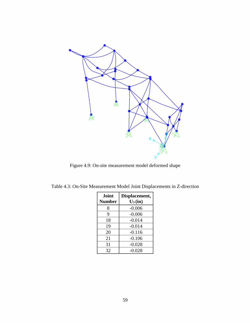
Figure 4.9: On-site measurement model deformed shape ............................................................ 59

Figure 4.10: Plan view base dimensions: (a) Original point cloud; (b) Structural plans .............. 61

Figure 4.11: (a) New point cloud base dimensions; (b) On-site base dimensions ........................ 62

Figure 4.12: Original Point Cloud Elevation ................................................................................ 63

Figure 4.13: Structural plan elevation ........................................................................................... 63

Figure 4.14: New point cloud elevation ........................................................................................ 64

Figure 4.15: On-site measurement elevation ................................................................................ 64

Figure 4.16: Ranges and averages of displacement percent difference given by the three data

sources when compared to the on-site model ............................................................................... 74

Figure 4.17: Ranges and averages of base reaction percent difference given by the three data

sources when compared to the on-site model ............................................................................... 75

Figure 5.1: Image from SAP2000: Undeflected frame model ...................................................... 77

xii

Figure 5.2: Dead and live load on structural plan model .............................................................. 78

Figure 5.3: Deformed shape of structural plan model after loads are applied. Maximum

deflection occurs at the node 94 circled in red having a value of U3 = -3.6613 in ....................... 79

Figure 5.4: Base joint labeling for bridge models......................................................................... 79

Figure 5.5: Structural Plans - (a) Mode Shape 1; (b) Mode Shape 2 ............................................ 81




Figure 5.9: Structural Plans - Mode Shape 9 ................................................................................ 83

Figure 5.10: Deformed shape fine point cloud after loads are applied. Maximum deflection

occurs at the node 94 circled in red having a value of U3 = -3.5274 in ....................................... 87

Figure 5.11: Deformed shape of medium point cloud after loads are applied. Maximum

deflection occurs at the node 93 circled in red having a value of U3 = -3.0287 in ...................... 87

Figure 5.12: Deformed shape of coarse point cloud after loads are applied. Maximum deflection

occurs at the node 94 circled in red having a value of U3 = -3.4688 in ....................................... 87

Figure 5.13: Fine Point Cloud - (a) Mode Shape 1; (b) Mode Shape 2; (c) Mode Shape 3 ......... 89



Figure 5.16: Medium Point Cloud - (a) Mode Shape 1; (b) Mode Shape 2; (c) Mode Shape 3 ... 91

Figure 5.17: Medium Point Cloud - (a) Mode Shape 4; (b) Mode Shape 5; (c) Mode Shape 6 ... 91

Figure 5.18: Medium Point Cloud - (a) Mode Shape 7 (b) Mode Shape 8; (c) Mode Shape 9 .... 91

Figure 5.19: Coarse Point Cloud - (a) Mode Shape 1; (b) Mode Shape 2; (c) Mode Shape 3 ..... 92

xiii



Figure 5.22: Ranges and averages of frequency percent differences when comparing the three

point clouds to the structural plans ............................................................................................. 110

Figure 5.23: Experimental data run in Matlab – (a) Mode Shape 1; (b) Mode Shape 2; (c) Mode

Shape 3; (d) Mode Shape 4; (e) Mode Shape 5 .......................................................................... 112

Figure 5.24: (a) Mode shapes move similarly since only 6 sensors are being used; (b) Additional

sensors on the same structure show more truthful mode shapes and their apparent differences 113

Figure 5.25: MAC - Experimental mode shapes vs. Structural plan mode shapes ..................... 115

Figure 5.26: Mode shape 2 of the structural plans and mode shape 1 of the experimental data

showing identical movement bending in the Z-direction at nearly identical frequencies .......... 117

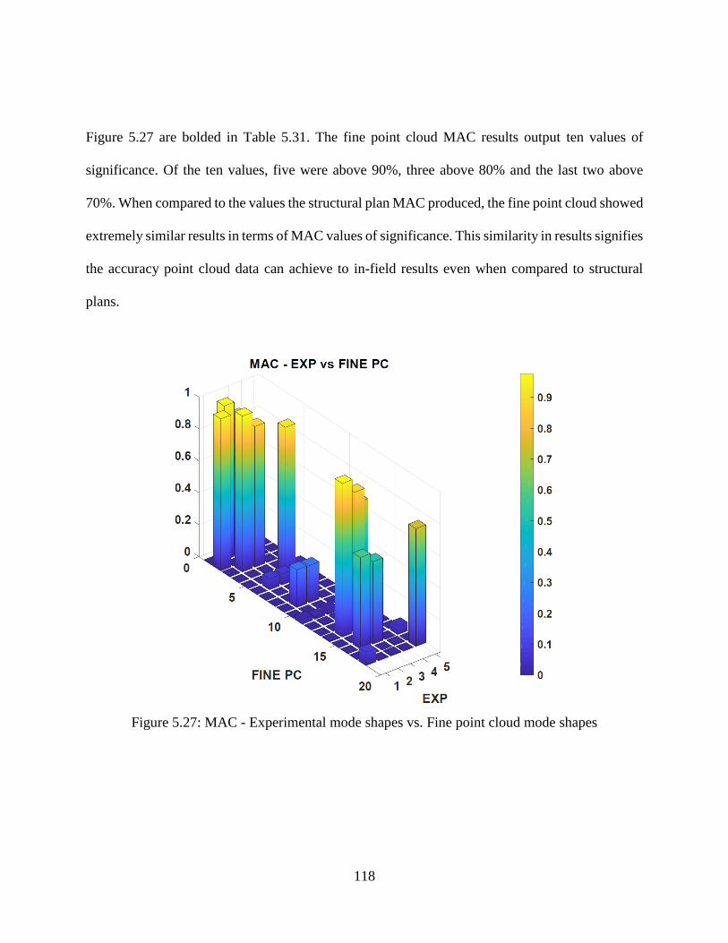
Figure 5.27: MAC - Experimental mode shapes vs. Fine point cloud mode shapes .................. 118

Figure 5.28: Mode shape 3 of the fine point cloud and mode shape 2 of the experimental data

showing similar movement of torsion about the x-axis with frequencies in close proximity .... 120

Figure 5.29: MAC - Experimental mode shapes vs. Medium point cloud mode shapes ............ 121

Figure 5.30: Mode shape 3 of the fine point cloud experimental data showing similar movement

of torsion about the x-axis with frequencies within approximately 13% of each other ............. 124

Figure 5.31: MAC - Experimental mode shapes vs. Coarse point cloud mode shapes .............. 125


showing similar movement of out-of-phase bending in the Z-direction with a frequency

difference of less than 8% ........................................................................................................... 128

xiv

LIST OF TABLES

Table 4.1: New Point Cloud Joint Displacements in Z-direction ................................................. 56

Table 4.2: New Point Cloud Joint Reactions in Z-direction ......................................................... 56

Table 4.3: On-Site Measurement Model Joint Displacements in Z-direction .............................. 59

Table 4.4: On-Site Measurement Model Joint Reactions in Z-direction ...................................... 60

Table 4.5: Member Size Comparison: Structural Plans vs. New Point Cloud ............................. 66

Table 4.6: Displacement comparison between point cloud models .............................................. 67

Table 4.7: Displacement comparison between original point cloud and structural plans ............ 67

Table 4.8: Percent difference between new point cloud and structural plans ............................... 68

Table 4.9: Joint Displacement Comparison - On-Site Model vs. Original Point Cloud ............... 69

Table 4.10: Joint Displacement Comparison - On-Site Model vs. Structural Plans ..................... 69

Table 4.11: Joint Displacement Comparison - On-Site Model vs. New Point Cloud .................. 70

Table 4.12: Reaction comparison between point cloud models ................................................... 71

Table 4.13: Reaction comparison between structural plans and original point cloud .................. 71

Table 4.14: Reaction comparison between structural plans and new point cloud ........................ 72

Table 4.15: Base Joint Reaction Comparison - On-Site Model vs Original Point Cloud ............. 73

Table 4.16: Base Joint Reaction Comparison - On-Site Model vs Structural Plans ..................... 73

Table 4.17: Base Joint Reaction Comparison - On-Site Model vs New Point Cloud .................. 73

Table 5.1: Member Sizes Given by Structural Plans .................................................................... 76

Table 5.2: Base Joint Reactions for Structural Plans .................................................................... 80

Table 5.3: Structural Plans - Modal Periods, Frequencies and Eigenvalues ................................ 84

xv

Table 5.4: Structural Plans - Load Participation Factors .............................................................. 84

Table 5.5: Base Joint Reactions for Fine Point Cloud .................................................................. 88

Table 5.6: Base Joint Reactions for Medium Point Cloud ............................................................ 88

Table 5.7: Base Joint Reactions for Coarse Point Cloud .............................................................. 88

Table 5.8: Fine Point Cloud - Periods, Frequencies and Eigenvalues .......................................... 90

Table 5.9: Fine Point Cloud - Load Participation Factors ............................................................ 90

Table 5.10: Medium Point Cloud - Periods, Frequencies and Eigenvalues.................................. 92

Table 5.11: Medium Point Cloud - Load Participation Factors .................................................... 92

Table 5.12: Coarse Point Cloud - Periods, Frequencies and Eigenvalues .................................... 93

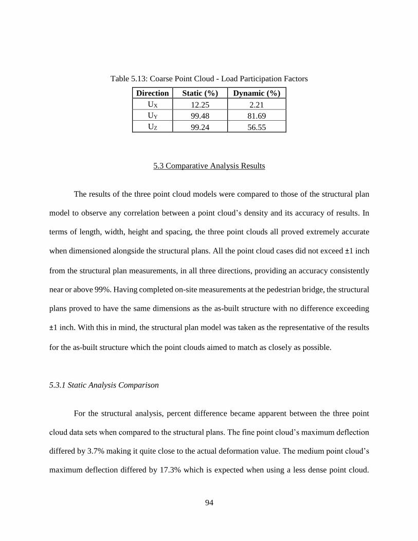
Table 5.13: Coarse Point Cloud - Load Participation Factors ...................................................... 94

Table 5.14: Base Joint Comparison: Structural Plans vs Fine Point Cloud .................................. 95

Table 5.15: Base Joint Comparison: Structural Plans vs Medium Point Cloud ........................... 95

Table 5.16: Base Joint Comparison: Structural Plans vs Coarse Point Cloud .............................. 96

Table 5.17: Member Size Comparison - Fine Point Cloud vs. Structural Plans ........................... 98

Table 5.18: Result Comparison - Fine Point Cloud vs. Structural Plans ...................................... 99

Table 5.19: Load Participation Comparison - Fine Point Cloud vs. Structural Plans ................ 100

Table 5.20: Member Size Comparison - Medium Point Cloud vs. Structural Plans .................. 102

Table 5.21: Results Comparison - Medium Point Cloud vs. Structural Plans ............................ 103

Table 5.22: Load Participation Comparison - Medium Point Cloud vs. Structural Plans .......... 104

Table 5.23: Member Size Comparison - Coarse Point Cloud vs. Structural Plans ..................... 105

Table 5.24: Results Comparison - Coarse Point Cloud vs. Structural Plans .............................. 106

Table 5.25: Load Participation Comparison - Coarse Point Cloud vs. Structural Plans ............ 107

xvi

Table 5.26: Point Cloud Frequency Comparison - Fine vs Medium .......................................... 108

Table 5.27: Point Cloud Frequency Comparison - Fine vs Coarse ............................................. 108

Table 5.28: Point Cloud Frequency Comparison - Medium vs Coarse ...................................... 109

Table 5.29: MAC values for Experimental mode shapes vs. Structural plan mode shapes ....... 116

Table 5.30: Frequency Comparison via MAC value - Experimental vs Structural Plans .......... 117

Table 5.31: MAC values for Experimental mode shapes vs. Fine point cloud mode shapes ..... 119

Table 5.32: Frequency Comparison via MAC value - Experimental vs Fine Point Cloud ........ 120

Table 5.33: MAC values for Experimental mode shapes vs. Medium point cloud mode shapes

..................................................................................................................................................... 122

Table 5.34: Frequency Comparison via MAC value - Experimental vs Medium Point Cloud .. 123

Table 5.35: Frequency Comparison via MAC value - Experimental vs Medium Point Cloud

(Adjusted) ................................................................................................................................... 124

Table 5.36: MAC values for Experimental mode shapes vs. Coarse point cloud mode shapes . 126

Table 5.37: Frequency Comparison via MAC value – Experimental vs Coarse Point Cloud .... 127

Table 5.38: Frequency Comparison via Mac Value - Experimental vs Coarse Point Cloud

(Adjusted) ................................................................................................................................... 127

17

CHAPTER 1 – INTRODUCTION

In today’s growing construction era, developing more efficient and effective products of

high quality is paramount; therefore, there is a need for more modern technologies such as finite

element analysis (FEA) software and three-dimensional laser scanning. These modern

technologies play a big role in the applications of civil infrastructure design, maintenance,

operation and as-built construction verification. Advancements in possible analysis alternatives,

such as point cloud data collection, have become of great interest to engineering practice and

research due to the potential this technology possesses.

1.1 Objectives

Structural plans are the standard source of data for FEA modeling within the realm of

engineering. This report intends to evaluate the plausibility of point cloud technology as a tool that

provides accurate results when analyzing existing structures. The static behavior of a section of a

steel-reinforced football stadium and the static and dynamic properties of a pedestrian bridge, both

located on the University of Central Florida (UCF) campus, will be studied. By using a 3D laser

scanner, point cloud data will be obtained and stitched together to create a 3D image capable of

being imported into an FEA program.

Moreover, the stadium results will be compared to a previous study that provides the

structural plans and the point cloud data. To understand the accuracy point cloud technology can

deliver, the new study will compare results found by different users, structural plans and actual

on-site measurements. The bridge will also have a comparative analysis using the original

18

structural plans versus three levels of point cloud densities: Fine, Medium and Coarse. The results,

consisting of displacements and reactions for static analysis and mode shapes, periods, frequencies

and eigenvalues for dynamic modal analysis, will be determined through FEA software. The

Modal Assurance Criterion (MAC) will also be utilized so as to compare the four data sources of

the pedestrian bridge against actual experimental data gathered in the field. The results will give

readers an indication of the ability point cloud technology has, whether it is feasible to use and

how density affects results.

1.2 Scope

Using the data collected via the sources mentioned in Section 1.1, the respective computer

models of each data source will be created in order to complete analyses by the FEA program.

Several programs are needed to complete the project and are listed as follows: Autodesk Recap,

Autodesk Inventor, AutoCAD, SAP2000 and MATLAB. Using the same structures when

comparing two different sets of data sources allows for a fair comparison of results, both static and

dynamic. The analysis of the stadium and bridge will be simplified by solely including their steel

framing. The concrete footings for Spectrum Stadium are represented as pinned supports and the

concrete abutments for the pedestrian bridge are represented as fixed supports.

19

1.3 Description of Scanned Structures

1.3.1 Spectrum Stadium

Spectrum Stadium is located at the northeast of the UCF campus alongside North Orion

Boulevard. The stadium is a predominately steel structure capable of holding over 45,000 people.

The stadium is mainly supported through a system of wide flanged beams and columns that is

arranged around the entire structure. The purpose of this structure is to operate as the location of

home games for the UCF football team. Refer to Figure 1.1 for a photo of Spectrum Stadium.

Figure 1.1: Spectrum Stadium on UCF campus

Source: UCF Facilities

http://ucfknights.com/ViewArticle.dbml?DB_OEM_ID=34100&ATCLID=211735275

http://ucfknights.com/ViewArticle.dbml?DB_OEM_ID=34100&ATCLID=211735275

20

1.3.2 Pedestrian Bridge

Parking Garage VI – H Pedestrian Bridge is located near the CFE Arena on Gemini

Boulevard North on the UCF Campus. This pedestrian bridge is a steel truss bridge with a

reinforced concrete deck. It is 177 feet long by 12 feet wide and comprised of three spans. The

bridge mainly facilitates the movement of pedestrians and small utility vehicles. Essential steel

components of this bridge are comprised of HSS and W-sections. Refer to Figure 1.2 for a photo

of the pedestrian bridge.

Figure 1.2: Parking Garage VI – H Pedestrian Bridge on UCF campus

21

CHAPTER 2 – LITERATURE REVIEW

2.1 Point Cloud Technology

A point cloud is a set of data points in space. Point clouds are generally produced by 3D

Light Detection and Ranging (LiDAR) scanners, which measure numerous points on the external

surfaces of objects around them [1]. Each of these points in space provide an individual 3D

coordinate by supplying their X, Y and Z position values. Point clouds can be used as a reference

to recreate existing structures or insert additional models [2]. Attaching a point cloud into a

compatible software allows it to be used as a guide for drawing, display changes or color stylization

that can demonstrate different features of the structure [2].

There are several methods of point cloud data collection that can be utilized via the use of

laser scanners: stationary 2D and 3D, phased-based, time of flight, mobile and airborne [3]. Point

clouds have numerous purposes including creating 3D CAD models for manufactured parts,

metrology, quality inspection, visualization, animation, rendering and mass customization

application [4]. Having used a 3D laser scanner in this study, the pros and cons that accompany

the tool becomes crucial before determining its appropriateness for a project. Once a user

recognizes the capabilities and limitations of this powerful tool, an educated decision can be made

regarding the suitability of the scanner. The following pros and cons are just some of the traits that

come with using a LiDAR scanner:

Pros:

• Faster data capture times when compared to typical structural measuring techniques

22

• Effective data collection reducing the amount of on-site visits

• Unobtrusive data collection method, eliminating the need for hands-on or invasive

techniques

• Highly precise and accurate measurements

• Leads to a lower transfer cost due to small number of resources for data acquisition

thus leading to higher productivity

• Illustrates the structural space in 3D as opposed to the normal 2D display of

measurements in structural plans

Cons:

• High initial investment

• Requirement of purchase and training of the new software to be used for the

creation of point clouds

• High-end and sophisticated hardware for data processing

• Susceptible to technical errors that could delay projects

2.2 Leica Scanner

The device used for the pedestrian bridge scan was a Leica ScanStation P-Series 3D laser

scanner. The scanner has impressive capabilities including being operated for a variety of uses

such as capturing 3D geometry of civil infrastructure, 3D data integration for Building Information

Modelling (BIM) and re-constructing crime scenes [5]. The instrument is able to scan at a rate of

1 million points per second and has the capability to capture surfaces from a distance up to 270 m

away [5]. It is durable enough to function in temperatures ranging from -20°C to +50°C, compliant

23

with the IP54 ratings for dust and water resistance, demonstrates survey grade dual axis

compensation and delivers low range noise [5]. The advantages of this system are its high speed,

precision and range for challenging projects.

2.2.1 Basic Principle of Laser Scanning

The scanner works by emitting a light signal (laser) through a transmitter and receiving the

return signal by a receiver [6]. Today, there are two typical scanner types used which are defined

by the technique they use for their distance calculation [6]. The first scanner type is known as

‘Time of Flight’ which uses a distance calculating technique based on the time elapsed between

the emission of the laser and the reception of the return signal [6]. The second scanner type is the

‘Phase-Based’ which calculates distance by comparing the phases of the output signal and the

return signal [6]. Overall, time of flight scanners tend to scan slower than phase-based scanners

but can scan farther while phased based scanners tend to scan faster but are limited in scanning

range [7]. Figure 2.1 gives an illustration of the difference between the two techniques.

24

Figure 2.1: Scanner Distance Calculation Techniques: Time of Flight vs. Phased-Shift Based

Source: SurvTech Solutions

http://floridalaserscanning.com/3d-laser-scanning/how-does-laser-scanning-work/

Figure 2.2 shows a diagram of a typical laser scanner. The emitter is seated on the body

while he body rotates around the axis vertically which also consists of a horizontally rotating

mirror [6]. This mirror reflects the laser and directs it towards a detected surface point [6]. These

movements occur at extremely high speed which then lead to accelerated data acquisition [6]. This

ability entices the use of these tools since they can collect both millions of data points in seconds

while also providing powerful accuracy.

http://floridalaserscanning.com/3d-laser-scanning/how-does-laser-scanning-work/

25

Figure 2.2: Anatomy of a 3D laser scanner

Source: 3DSCAN

http://www.3dscan.it/en/blog/how-does-it-work-a-3d-laser-scanner/

2.2.2 Image Acquisition and Parameters

The resolution of a scan can be established by the speed and pitch of rotations given by the

user [6]. The slower a scanner rotates, the denser the point cloud becomes due to the amount of

grid points acquired. The denser a point cloud is, the better the quality of data collected. The

computed distance, vertical angles and horizontal angles are based on the position of the mirror

and body for each measured point [6]. The value of reflectance of surface is also acquired and is

usually higher when the surface is white [6]. Reflectance can at times become a hindrance when

scanning highly reflective materials such as windows or mirrors. This issue with shiny surfaces is

what is known as ‘noise’ [8].

These parameters can be affected by several settings input by the user. An example of a

simple parameter input by the user is deciding between scanning a small angle wedge or 360°.

http://www.3dscan.it/en/blog/how-does-it-work-a-3d-laser-scanner/

26

Parameters can also differ depending on the type of LiDAR system a user is equipped with; for

example, if dealing with an airborne scanner the scanning pattern becomes a factor that is not

present when using a stationary 3D laser scanner [9]. An example of these scanning patterns can

be seen in Figure 2.3.

Figure 2.3: Scanning patterns for airborne LiDAR

Source: USDA – Forest Service

https://www.fs.fed.us/pnw/pubs/pnw_gtr768.pdf

A digital camera is integrated within the laser scanner in order to collect images of the

areas scanned [6]. The purpose of these cameras is to allow a user to use the color collected through

the images captured and input them into the point cloud [6]. This option is ideal for the archiving

of structures since it allows the point cloud to have a greater photo-realistic look. Once all these

capabilities have been applied by a user, depending on their goal, they can use the point cloud to

output 2D and 3D deliverables [6].

https://www.fs.fed.us/pnw/pubs/pnw_gtr768.pdf

27

2.3 Modal Dynamic Analysis

2.3.1 General Overview

The dynamic analysis of a structure produces several results such as natural frequency,

displacements, time history outputs and modal shapes [10]. In the real world, every structure

undergoes dynamic loading [10]. The internal stresses of structures and their resulting deflection,

due to this loading, are time dependent or dynamic in nature since load application and removal

varies with time [11]. Modal dynamics, specifically, determines the frequencies and mode shapes

of a structure and depend on the mass, damping and stiffness distribution of the system [10].

Anything that possesses mass and elasticity is inclined to vibration and therefore behaves in an

oscillatory nature [11].

2.3.2 Types of Vibrations

Generally, the types of vibrations fall within two categories: free and forced. Free vibration

occurs when a structure is disturbed from its static equilibrium and allowed to vibrate without an

external force being applied [12]. Free vibration is the type of vibration that was considered for

the study described in Chapter 5. A structure that undergoes free vibration will vibrate at one or

more of its natural frequencies depending on the mode that is being studied [11]. The equation of

motion for free vibration is shown in Equation 1. The variables in Equation 1 are listed as follows:

[ 𝑚 ] = mass matrix, [ 𝑐 ] = damping matrix, [ 𝑘 ] = stiffness matrix, { �� } = acceleration, { �� } =

velocity and { 𝑢 } = displacement. If the system has n degrees of freedom, the size of [ 𝑚 ], [ 𝑐 ],

and [ 𝑘 ] is [n x n]. If a system has anything more than one degree of freedom, it is considered a

28

multiple degree of freedom system [10]. When no damping is present, the [ 𝑐 ] has no value

therefore rendering it negligible. The equation of motion for an undamped system can be written

as shown in Equation 2.

[ 𝑚 ] { �� } + [ 𝑐 ] { �� } + [ 𝑘 ] { 𝑢 } = { 0 } (1)

[ 𝑚 ] { �� } + [ 𝑘 ] { 𝑢 } = { 0 } (2)

The second type of vibration occurs under the influence of external forces and thus named

forced vibration [12]. A condition known as resonance occurs when the frequency of the external

force matches the natural frequency of the structure [11]. This coinciding of frequencies causes

significant deformations for structures which could ultimately lead to critical failure [11]. The

equation of motion for forced vibration is shown in Equation 3. The new variable in this equation,

when compared to free vibration, is P(t). This variable represents the external force acting on a

system and differentiates forced vibration from free vibration. Should damping not be present, it

would similarly be neglected as it was in Equation 2.

[ 𝑚 ] { �� } + [ 𝑐 ] { �� } + [ 𝑘 ] { 𝑢 } = 𝑃(𝑡) (3)

2.4 Prior Work

Research into the feasibility of point cloud technology as a tool for model reconstruction

has been and still is being completed. [13] evaluated the accuracy of deformation of a structure

29

using two point clouds, one with the undeformed shape and the other with its deformed shape. The

study concluded that this point cloud comparison gave a measurement accuracy of ± 0.2 mm (95%

confidence interval) [13]. Much research has been completed on the accuracy of the scanner itself,

its ability to obtain real-life measurements and what factors contribute to the accuracy of the

results. [14] explains that decisions made during the ‘registration’ of a point cloud have a direct

impact on the accuracy point cloud dimensions can produce. The topic of point cloud registration

is further discussed in section 3.3 of this thesis.

Lastly, studies on digital photogrammetry, such as laser scanning, when compared to

traditional measuring techniques have been completed. Research completed by [15] showed the

percent differences found when photogrammetry techniques were compared to both typical hand

measurements and structural plan designs. The study found that photogrammetry only differed

from a range of 0.06% - 1.43% when compared to hand measurements and 0.23% - 8.00% when

compared to structural plan dimensions [15]. Similarly, dimensional comparisons where

completed for the structures mentioned in this thesis to further understand the uncertainty expected

when using this technology.

30

CHAPTER 3 – METHODOLOGY

According to the American Society of Engineering Education, one of the basic objectives

within engineering is the detailed comprehension of the engineering method and an elementary

aptitude in its application [16]. The methodology of this study focuses on a need and problem point

cloud technology could potentially serve. Through this narrowed emphasis, an essential question

was framed: could point cloud modeling be used as an alternative to structural plans? The need for

such a substitute was explored in-depth by defining potential issues point cloud technology could

help mitigate. The main issue examined, regarding engineering, is what to do should structural

plans not be available in time-sensitive cases or if the as-built structure differed from what was

shown in the structural plans.

Time-sensitive cases are highlighted in situations such as post-disaster structural integrity

assessments. For these assessments, time plays an essential role for engineers in determining

whether structures are on the brink of critical failure and are a risk to public safety. The use of

point cloud technology is already utilized in post-disaster assessments by the Federal Emergency

Management Agency (FEMA) due to the large-scale areas LiDAR scanners can map out [17]. This

real-world application emphasizes the need for such technology in the ability to assess structures

within engineering.

With the goal of this study aiming to assess the viability of point cloud technology, a

quantitative approach was undertaken as the appropriate course of action. This approach was

chosen due to the need for engineers to quantify the integrity of structures through numeric

measurements and calculations. As mentioned in Section 2.2, a LiDAR scanner was used for this

31

study but its sole purpose was to collect the points that make up the point cloud data. The other

essential tools used for this study are computer programs such as Cyclone Register 360, Autodesk

Recap, AutoCAD, SAP2000 and MATLAB. Of all the programs, Cyclone Register 360 is the only

program capable of registering the point cloud data collected by the scanner since it is made by

the same company that manufactures the laser scanner.

3.1 Surface Reconstruction and Modeling

The goal of using a laser scanner is to regenerate structures seen in the field to a point cloud

model with surfaces that are tangible enough for software to read. In order to reconstruct these

surfaces, a set of sample points is collected by the laser near a structure’s surface and recreated as

closely as possible within the software [18]. It is impossible to obtain 100% accurate regeneration

considering only a finite set of sample points can be collected by a laser, but the greater amount of

data points collected the higher the accuracy [18]. The more points collected, the denser a point

cloud becomes which allows for better recreation of the real-life structure [18].

The best collection of data points a user can have is when the essential areas are given high

density while the featureless areas are limited in data point collection [18]. A multitude of factors

can affect the collection of these data points which in turn, affect the quality of model generation.

These factors can be things such as scan time for density, type of surfaces, noise level and

obstructions. Since these factors play a role in accuracy, it is important that the appropriate

algorithm program be used for the reconstruction method [18]. Once such a program is chosen, a

user will be able to garner the correct geometry, features and topology through the sample data

points collected [18].

32

3.2 Classification of the Reconstruction Algorithms

The classification of the reconstruction methods is a complex process due to the amount of

methods and their respective subcategories. According to [19] and [20], there are five major

categories for algorithm reconstruction: spatial subdivision, surface construction with distance

functions, surface construction by warping, incremental surface-oriented construction and

clustering. Each of the five categories have individual methods within them found through the

work of an assortment of researchers.

The first major category, known as spatial division, enlists two subcategories called

surface-oriented cell selection and volume-oriented cell selection [20]. This category is the only

of the five to also have two subcategories that contain different approaches. The two subcategories

have general steps that are followed, respectively, but have been applied with different techniques.

An example of a different technique is found in [21], where a distance function was applied within

the surface-oriented cell selection approach. This technique is also notable for being able to fall

into the second major category: surface construction with distance functions [19]. For the volume-

oriented approach, Boissonat’s approach is seen throughout research works but is not the only

method used; for example, [22] demonstrates an approach that differs from Boissonat’s by being

able to fill any holes on the surfaces collected. This new technique becomes beneficial, considering

Boissonat’s approach only works for surfaces that do not have any holes [21]. Figure 3.1 displays

the approach detailed in [22] where holes on surfaces are filled in through their algorithm process.

33

Figure 3.1: Volume-Oriented approach demonstrating holes in surfaces being filled in

Source: Brian Curless and Marc Levoy

Surface construction with distance functions is the second major algorithm category. As

mentioned earlier, one of these approaches is also found in [21]. Although it is used within the

spatial division category, the approach utilizes distance functions therefore making it applicable to

this category as well. These types of category-bending approaches add to the complexity of the

classification of these techniques. The third major category is surface construction by warping

which, given its name, is self-explanatory. This technique deforms an initial surface in order to

34

approximate, to the best of one’s ability, the given data points collected through scanning [19]. An

example of this approach is seen through spatial free form warping which warps the entire space

an object is fixed in while simultaneously warping the object congruently [19].

Incremental surface-oriented construction is the fourth major category for algorithm

reconstruction. As defined by [20], “the idea of incremental surface–oriented construction is to

build up the interpolating or approximating surface directly on surface–oriented properties of the

given data points.” This approach is illustrated in Figure 3.2. An example of this method is

Boissonat’s surface approach which adds to the category-bending complexity mentioned in the

second major category. This approach uses localized Delaunay triangulation as seen in Figure 3.2

as well [20].

(a) (b)

Figure 3.2: (a) Basic principle of incremental surface-orientation; (b) Boissonat's surface-

oriented approach

Source: Robert Mencl

Lastly, the fifth and final major category is known as clustering. This approach is taken

when multiple shapes are connected and represented in a set of collected data points [19]. This

35

method becomes useful as the previous categories are meant more for data representing one shape

[20]. In most cases, as in this study, a structure will not be limited to one shape but have several

shapes interconnected. Clustering eases this issue by segmenting a set of sample points into a

subdivision of points that belong to the same component [20]. Although these five major categories

are the standard methods used today, research into new categories and new approaches within the

established methods is constant.

3.3 Registration Theory

When attempting to obtain a point cloud from an existing structure, generally, more than

one scan shall be necessary for the cloud to be considered suitable. The process known as

registration regards the joining or stitching together of individual scans into one comprehensive

point cloud [23]. For every scan, the center scan location (0, 0, 0 for x, y, z) is at the mirror

embedded within the scanner where the laser beam strikes [23]. If the scanner is moved to different

locations, each scan location has its own individual center which has to be aligned in order to

properly register the point cloud [23]. To stitch together these scans, the overlapping points have

to be matched as perfectly as possible in order to create proper alignment [24].

So as to complete an acceptable registration, [23] states “a minimum of three corresponding

points, not on the same line, are required to compute the six rigid-body-transformation parameters

needed to translate and rotate a secondary point cloud to a primary one.” The more corresponding

points you obtain, the more accurate your overall point cloud will be [23]. The goal of these

correspondents is to optimize both sets of point cloud scans until they are stitched together with as

minimal distortion as possible [23]. Figure 3.3 demonstrates how several scans completed at

36

different angles are registered into one comprehensive point cloud. The stitching together of two

point cloud scans is known as pairwise registration and the steps to complete these steps can be

seen in Figure 3.4 [24]. Many factors can affect the accuracy of the registration as concluded in

[14]. Decisions in the inclusion of intensity values and/or color features directly affect registration

accuracy [14].

(a)

(b)

Figure 3.3: (a) Individual point cloud scans; (b) Stitched together comprehensive point cloud

Source: Point Cloud Library

http://pointclouds.org/documentation/tutorials/registration_api.php


37

Figure 3.4: Pairwise registration steps flowchart

Source: Point Cloud Library


There are two important methods to find the correspondences between the overlapping

scanned data: target-based and targetless registration [23]. For target-based registration, artificial

targets are the common tool used within the field and it was the tool used for both studies in

Chapter 4 and 5. Natural targets can be used but tend to be more challenging and dependent on

human judgment [23]. The two main types of artificial targets are highly reflective spheres and

black and white planes [23]. The spheres were used for the study done in Chapter 4 and the black


38

and white planes were used for the study done in Chapter 5. Note that since the targets are placed

within the field of view of the scanner, additional time has to be taken during the registration

process to remove the points representative of the targets within the point clouds.

For targetless registration, the registration process is divided into two steps: coarse and fine

registration [23]. The fact that a single point cloud is capable of containing millions of points, the

task of matching two point clouds with millions of points would prove too tedious to be useful

[23]. In order to mitigate this issue, two coarse point clouds containing significantly fewer points

are matched in order to have a basis for the matching of the fine point cloud containing all the

points collected [23]. This method is useful to make the computation of the registration more

efficient should targets not be used in the field.

3.4 Data Collection

3.4.1 Spectrum Stadium Data

The point cloud data for Spectrum Stadium was collected by Sofia Baptista and Jacob

Solomon with the assistance of the UCF Institute for Simulation and Training (IST). This data was

gathered and expanded on in a term paper written by both Ms. Baptista and Mr. Solomon.

According to the authors, a FARO Focus3D S120 terrestrial laser scanner was the instrument used

to collect the point cloud data [25]. Due to many visual similarities within the support system of

the stadium structure, the authors utilized ‘tracking balls,’ shown in Figure 3.5, as artificial targets

to help mitigate the issue [25]. The tracking balls work as a reference system for the scanner by

helping to ease the registration process within the software once the scans are uploaded. In total,

39

four 360-degree scans were performed on-site [25]. The location of the stadium section scanned

can be seen in Figure 3.6. Figure 3.7 highlights the limits of framing support chosen within that

section of the stadium. Once completed, the scans were assembled, processed and imported into

Autodesk Recap.

Figure 3.5: Tracking balls used on-site

Source: Sofia Baptista and Jacob Solomon

40

Figure 3.6: Section of Spectrum Stadium scanned shown in red

Source: Sign posted within Spectrum Stadium

Figure 3.7: Limits of scan area shown by red lines. Marks 1-4 indicate the four scanning

locations.


41

Once the four scans were in Recap, they were combined into a single point cloud to

maximize detail to begin rendering section members. The Recap point cloud was then imported

into Autodesk Revit to overlay structural elements onto the point cloud visual to the best of the

user’s ability. The authors stated that the process was too difficult for them to render accurate

member sizes so they defaulted to the member sizes given in the structural plans. Once completed,

the rendered elements were imported into SAP2000 to complete a static analysis of the structure.

The process used by the authors of the original study can be seen in a simplified manner in Figure

3.3. Using the data provided by this term paper, the process to model and analyze the structure via

the point cloud files, supplied by Ms. Baptista and Mr. Solomon, was repeated but in a slightly

different manner as explained in Chapter 4.

Figure 3.8: Site to model analysis workflow


42

3.4.2 Pedestrian Bridge Data

Point cloud scanning of Parking Garage VI – H Pedestrian Bridge was completed with the

aid of Dr. Lori Walters and Mr. Rob Michlowitz from the UCF IST. Assistance with time

scheduling, photo documentation and note-taking were also provided by fellow classmates Paulo

Dos Santos, Samantha Weiser and Pruthviraj Thakor. A Leica ScanStation P-Series 3D laser

scanner was used for this study and provided by IST. The initial scanning attempt of the bridge

was interrupted due to technical difficulties with the laser scanner. Three scans had been completed

prior to the scanner’s software error but as a result, the scans were forced to be deleted through a

software reboot since it was the only way to mitigate the issue. The bridge scan was forced to be

postponed and rescheduled due to the issue.

Prior to arriving on-site for the second scanning attempt the following week, the scanner’s

software was updated and the initial calibration of the scanner was completed to save time.

Throughout the second on-site scanning attempt, a scanning time log, shown in Appendix A, was

created and includes the overall start time, end time, scanner setup time, scanning time and marking

targets. Scanning locations are also detailed on an aerial view of the site shown in Appendix B

with corresponding photos.

3.4.2.1 Point Cloud On-Site Procedure

Before commencing the scans, three black and white artificial targets labeled 1, 2 and 3

were set up on the bridge at approximately equal increments. In general, the scanner must be able

to see at least two targets at a time. Targets must not be arranged in a straight line so that the

43

scanner has triangular coordination with the targets. All targets were set at a height of 6.5 feet from

the base which was a height chosen at the user’s discretion. The height of the targets was chosen

to ensure the scanner had a direct line of sight from each scanning location. Figure C.1 in Appendix

C shows the target set up process.

The scanner was then set up on the north side of the bridge as that was the designated

location for the first scan. When using a stationary laser scanner, it must be leveled on a tripod in

order to collect accurate data. The tripod used in this study was a Leica 670223 14ZJP-0000 which

was also provided by IST. The tripod was leveled with a smartphone leveling application before

attaching the scanner to it. The leveling of the scanner on the tripod itself was fine-tuned with the

scanner’s digital assistance screen. Appendix C Figure C.2 also displays the process of setting up

the scanner on the tripod.

Once the scanner was leveled on the tripod, the scanner was programmed with the name of

the project, image resolution required and white balance setting (i.e., sunny, cloudy, etc.). To

decrease the amount of time per scan, the scanner was programmed to ignore photo imagery (scan

only). This setting limits the scanner to collecting the point cloud data in greyscale because it

refrains from capturing photos of each scan view. Finally, the scanner was programmed with the

angle range that it should capture. The preceding steps are shown in Appendix C, Figure C.3.

When starting the scan at the first location, the screen of the scanner must be oriented on

its right side. For all wedge angle scans (scans that are not 360⁰ scans), the scanner’s peephole,

shown in Appendix C, Figure C.4, must be placed in the line of sight of the angle’s starting point.

Once in position, the user manually rotated the scanner using the peephole’s line of sight until an

end point was determined for the scan. From the pre-programmed resolution and manually set

44

range, the scanner is able to measure the angle and estimated the amount of time it would take to

scan said angle.

After the first scan was complete, targets were located manually and marked within the

scanner’s screen. The targets must always be captured by the scanner in the same order after each

scan. A minimum of two targets must be captured by the scanner per scan but for some of the

scans, all three targets were able to be marked allowing for more precision in terms of the scanner’s

location. Appendix C, Figure C.4 shows how the targets were marked on the scanning screen.

On the north side of the bridge, the scanner was relocated to two more locations. For each

scan, the process of leveling the scanner and setting the range was repeated followed by capturing

the targets after the scan was completed. At the third location, note that only two targets were

captured as opposed to three at the first two locations. This was due to the lack of clarity from

interference from a palm tree directly within the line of sight of the target. This issue gave the

scanner difficulty in distinguishing where the target ended and the palm tree began. The scanner

was then repositioned for one scan at the east end of the bridge, four different scans on the south

side of the bridge and one scan at the west end of the bridge. For each scan, the process of leveling

the scanner, setting the range, and capturing the targets was repeated.

Finally, the scanner was relocated to two separate locations on the bridge. Prior to the first

scan on the bridge, target 1 was relocated to the north side of the bridge. Moving a target is possible

if one of the other original targets is left in place and used as a reference point for the newly moved

target. For these two scans, manually dictating an angle wedge was unnecessary as the capture

range was set to 360 degrees. Overall, the entire process (11 scans total) took place over the course

of five hours and forty-five minutes.

45

3.4.2.2 Point Cloud Registration

After the on-site scanning, the scanner was taken back to the office of Mr. Michlowitz to

process the data and form a point cloud. In order to create a composite point cloud, Mr. Michlowitz

used the Leica program Cyclone Register 360 which is a 3D laser scanning point cloud registration

software. The software is programmed to accept the data collected from the Leica laser scanner

and gives users the ability to manipulate, edit and stitch together the scans while also obtaining a

registration report. Before any editing, the scans were opened in Cyclone Register 360 and

produced the 3D image seen in Figure 3.4. The registration report for the unedited scan can be

found in Appendix D.

Figure 3.9: Unedited composite point cloud scan in Cyclone Register 360

The stitching together of the 11 scans into one comprehensive point cloud was done via

the use of the target locations set up on site which allowed the program to use coordinate

triangulation. Dr. Walters noted that the use of targets cut software editing time by approximately

46

75% although increasing the scanning time on site. Figure 3.5 illustrates the locations the scanner

was placed given by the registration report in Cyclone Register 360. The green lines in the figure

indicate the strong links between the scanning locations (yellow triangles) which allowed scan

overlap, assisting a user in stitching the multiple scans together.

Figure 3.10: Scan locations diagram shown in Cyclone Register 360’s Registration Report

The amount of data points collected during the 11 scans included surfaces outside of the

bridge, leading to hefty file sizes exceeding over 24 gigabytes in total. These extra points are due

to the laser scanner’s ability to measure surfaces up to 270 meters away. The amount of points can

vary due to numerous factors such as scan angle and resolution choice. In this case, the lowest

number of points in a single scan was over 50 million while the higher end of the scans accrued

47

over 190 million points. In order to eliminate additional points that did not apply to the bridge, Mr.

Michlowitz used his expertise with Cyclone Register 360 to edit, trim and register the 11 scans.

Some of the elements that had to be trimmed out from the overall composite image are as follows:

trees/shrubbery, vehicles, buildings, people, reflection of the pond and the black and white targets.

Due to the amount of shrubbery at the site and its location in reference to the bridge, the

complete removal of the shrubbery from the point cloud was not plausible as shown in Figure 3.6.

Mr. Michlowitz indicated that the total time it took to register the point cloud was under two hours.

Cyclone Register 360 was able to precisely pinpoint the 11 locations the scanner was positioned

at to an accuracy of 7/16th of an inch. A zoomed-in image illustrating the density of the fine point

cloud can be seen in Figure 3.7. Following the registration, the process of preparing the point cloud

for dynamic model analysis began as expanded upon in Section 5.2.

Figure 3.11: Fine point cloud on Autodesk Recap following completed registration. Red arrow

indicates leftover shrubbery.

48

Figure 3.12: Zoomed-in fine point cloud on Autodesk Recap

49

CHAPTER 4 – SPECTRUM STADIUM STATIC ANALYSIS

4.1 Model Generation Using Point Cloud

As mentioned in Section 3.4.1, the original data collectors of the stadium point cloud data

completed a comparative study between the stadium’s structural plans and their interpretation of

the point cloud. In order to study if any accuracy differential exists when two users use the same

point cloud data, the study was repeated similarly with a few differences. The first difference was

that a model based on the on-site dimensions was created as a control in addition to the new point

cloud model. This was completed to compare the dimensions found by the point clouds as well as

those given in the structural plans. The measurements were gathered using a Bosch GLM 80

Lithium-Ion Laser Distance Measurer and a model was created using those measurements

alongside the member sizes provided by the structural plans.

Another difference that was noted in this study was the type of FEA program used to render

the member sizes. The original data collectors first used Autodesk Recap, then Autodesk Revit

and finally SAP2000 to analyze the point cloud. In the case of this study, Autodesk Inventor was

used as the FEA program of choice in lieu of Revit. The other programs described, Autodesk Recap

and SAP2000, were used in this study as they were in the original. The point cloud of the stadium

section used can be seen in Figure 4.1 when opened in Autodesk Recap. Lastly, [25] used the

section sizes provided by the structural plans due to difficulty rendering in Revit using the point

cloud. For this study, member sizes were rendered using the point cloud directly rather than

defaulting to the structural plans in order to see the uncertainty that might exist.

50

Figure 4.1: Point cloud of stadium section within Autodesk Recap

Inventor has similar capability to Revit in that it is used to render member sizes as closely

as possible to the point cloud visual that was imported. The following steps show a brief summary

of the procedure taken to render sections onto the point cloud visual within Inventor (Figures of

these steps can be seen in Appendix E):

1. Import Recap file into an Inventor “Assembly” file

2. Create a “Part” within the Assembly in order to create a 2D sketch on the sides of

point cloud

3. Insert a “Work Plane” on a flat surface of the users choosing to begin the 2D sketch

51

4. Using the point cloud as reference, create a center-to-center sketch by lining up the

sketch lines with the visible sections

5. Once the sketch is completed, insert frames and offset accordingly to match the

sections seen in the point cloud as best as possible. Users will have to take a trial-

and-error approach to determine the section size that they deem most similar to the

shape seen in the point cloud

6. Repeat the process for all applicable sides and sections of the structure

Once the sections were chosen and the point cloud had a fully rendered representation in

Inventor, the sketches were imported into AutoCAD. This step was necessary so that the sketch

could be input into SAP2000 since AutoCAD dxf files are compatible with SAP2000. Once the

sketches were in AutoCAD, the sketch was appropriately lined up ensuring that the frame lines

were connected and that there were no misalignments. The member sizes and length values are

entirely at the discretion of the user since they are dictated solely on a user’s judgment. For

example, if a sketch was measured in AutoCAD as having a length of 1200.34 inches, it is possible

for a user to assume that the member line had a length of 1200 inches. After completing this process

in AutoCAD, the dxf file was imported into SAP2000 for static analysis.

Once the frame drawing was transferred from AutoCAD to SAP2000, as seen in Figure

4.2, the program automatically labels each frame as a W18x35 member. Each frame had to be

manually changed and labeled to the appropriate member size as dictated by the rendering created

in Inventor. Once completed, seven equally spaced loads of 1.5 kips were placed on the horizontal

members seen in Figure 4.2. These applied loads acted as the static load on the structure to

complete the analysis for an output of deformations and reactions. These loads were chosen to

52

fully repeat the study completed by [25] and give a fair comparison without changing any of the

circumstances. The results of these load placements are seen in Section 4.2.

Figure 4.2: Images from SAP2000: (a) Undeformed frame shape; (b) Applied static loads on

horizontal members

4.2 Point Cloud Static Analysis Results

At the conclusion of the static analysis executed on the point cloud of a section of Spectrum

Stadium, the displacements of critical joints were obtained as well as the reactions at the pinned

joints. Prior to obtaining these outcomes, the lengths and widths of the pinned base joints were

found after completing the rendering of member sections in the point cloud. These base joint

distances were dimensioned to be compared to the previous case study with the elevations of the

53

structure also being compared. The base dimensions of the structure found through the new point

cloud can be seen in Figure 4.3 and the elevations in Figure 4.4.

Figure 4.3: Plan view of structure’s base points with accompanying dimensions based on the new

point cloud model

54

Figure 4.4: Elevation view of new point cloud model with accompanying dimensions

Once analyzed in SAP2000, the framing structure produced a deformed shape showing the

points of deflection as shown in Figure 4.5. The deformed shape is an exaggeration of the

deformation of the members as to emphasize where displacement occurs. In Figure 4.6, the image

establishes the joint labeling for referencing displacement to a respective node. The corresponding

deformations for said nodes can be seen in Table 4.1 while the base reactions are shown in Table

4.2. Both the displacements and reactions calculated are compared to the results found in both the

original study and the on-site measurements in Section 4.4. For both sets of tables, only the values

in the Z-direction were taken into account as was the case in the original study.

55

Figure 4.5: Deformed shape of new point cloud model after applying static load

Figure 4.6: Joint labeling via numbered nodes

56

Table 4.1: New Point Cloud Joint Displacements in Z-direction

Joint

Number

Displacement,

U3 (in)

8 -0.006

9 -0.006

18 -0.013

19 -0.013

20 -0.117

21 -0.110

31 -0.027

32 -0.027

Table 4.2: New Point Cloud Joint Reactions in Z-direction

Joint

Number

Reactions, R3

(kip)

1 8.09

2 7.37

11 18.38

12 17.68

24 28.38

25 28.18

4.3 On-Site Measurements Static Analysis Results

In the case of the model created by the on-site measurements, no rendering was needed as

the sections labeled within the structural plans were used in combination with the dimensions

found. The model was drawn directly in AutoCAD with the dimensions obtained and then

imported into SAP2000. As was shown for the point cloud model, the base joint dimensions and

the elevations of the structure from the on-site measurements are shown in Figure 4.7 and 4.8.

There comparative results with the rest of the models are seen in Section 4.4.

57

Figure 4.7: Plan view of structure’s base points with on-site dimensions

58

Figure 4.8: Elevation view of on-site measurement dimensions

After being analyzed, the model produced the deformed shape seen in Figure 4.9. Table

4.3 displays the displacements that coincide with the deformed shape and go by the same joint

numbering seen for the new point cloud in Figure 4.6. Both the new point cloud and the on-site

model results are compared to the original study in the following section.

59

Figure 4.9: On-site measurement model deformed shape

Table 4.3: On-Site Measurement Model Joint Displacements in Z-direction

Joint

Number

Displacement,

U3 (in)

8 -0.006

9 -0.006

18 -0.014

19 -0.014

20 -0.116

21 -0.106

31 -0.028

32 -0.028

60

Table 4.4: On-Site Measurement Model Joint Reactions in Z-direction

Joint

Number

Reactions,

R3 (kip)

1 8.57

2 7.86

11 18.25

12 17.72

24 27.26

25 26.91

4.4 Comparative Analysis of Stadium Results

4.4.1 Dimension Comparison

The results founded in this study varied in outcome when compared to the structural plans

of the stadium, the point cloud analysis completed in the original study and the in-field

measurements taken at the stadium. The initial comparison between all the model sources involves

the dimensions of the structure. Figure 4.10 shows the differences in length and width dimensions

between the original point cloud study and the structural plans. Figure 4.11 shows the difference

between the new point cloud study and the on-site measurements. Figures 4.12-4.15 show the

different elevation obtained through the different data sources. Overall, the percent difference

ranges and averages for the dimensions gathered by each data source, when compared to the actual

dimensions found on-site, are as follows:

o Original point cloud: Range = 0.5% - 10.0%; Average = 3.3%

o Structural plans: Range = 0.2% - 24.2%; Average = 5.0%

o New point cloud: Ranges = 0.2% - 8.0%; Average = 1.9%

61

Both point clouds fared far better than the structural plans most likely due to the as-built

structure undergoing adjustments during construction and/or renovations done over the years. With

the new point cloud averaging a 1.9% difference to the actual dimensions of the structure, point

cloud technology shows its ability to gather precise data.

(a) (b)

Figure 4.10: Plan view base dimensions: (a) Original point cloud; (b) Structural plans

Source: Sofia Baptista and Jacob Solomon [25]

62

Figure 4.11: (a) New point cloud base dimensions; (b) On-site base dimensions

63

Figure 4.12: Original Point Cloud Elevation


Figure 4.13: Structural plan elevation


64

Figure 4.14: New point cloud elevation

Figure 4.15: On-site measurement elevation

65

[25] notes that rendered the sections using the original point cloud was difficult enough to

be unsuccessful and resorted to using the sections provided by the structural plans. This is

important to note because it signifies that the only difference between the original point cloud and

the structural plans is the dimensions. Table 4.5 displays the differences in member sizes found

between the new point cloud and the structural plans. These differences are highlighted in yellow

alongside their respective cross-sectional area percent differences. The member sizes are classified

by their location via the joint labeling previously shown in Figure 4.6. As can be seen, the majority

of the member sizes differed from those seen in the structural plans. Although these member sizes

differed, it was realized that member size renderings for the new point cloud were within ± 2

section sizes of the member sizes given in structural plans and none exceeding a 30% difference.

The one exception to this finding was the horizontal frame spanning Joints 3-4. This exception is

due to the as-built section being a different member size than the one stated in the structural plans

accounting for the outlier in the comparisons. The average without this outlier, for percent

difference, was only about 13%.

66

Table 4.5: Member Size Comparison: Structural Plans vs. New Point Cloud

Frame Locations Structural

Plans New PC

Cross-Sectional

Area %

Difference

Vertical at Base Joints 1-2 W18x65 W18x55 16.4%



L-Diagonals L3x3x3/8 L3x3x3/8 0.0%

W-Diagonals at Joint 10 W8x28 W8x31 9.2%

W-Diagonals at Joint 15 W6x15 W6x20 29.1%

W-Diagonals between Joints 18 & 33,

19 & 34 W30x90 W30x90 0.0%

Horizontal at Joints 3-4 W18x35 W8x18 64.1%

Horizontals at Joints 8-9, 18-19 W18x65 W18x55 16.4%

Horizontals at Joints 20-23, 31-34 W16x40 W16x50 21.9%

Horizontal at Joints 13-14 W8x31 W8x40 25.0%

Horizontals between Joints 6 & 13,

7 & 14 W8x31 W8x31 0.0%

Horizontals between Joints 16 & 29,

17 & 30 W10x49 W10x45 7.9%

Average = 17.0%

True

Average= 13.0%

4.4.2 Displacement and Reaction Comparison

For the displacements, Table 4.6 pits the results founded from the original point cloud to

those of this study. As can be seen by the percentage differences, there was a varied gap of percent

difference ranging from nearly 0% to just under 30%. Similarly, Table 4.7 shows the displacement

percent difference between the point cloud from the original study and the structural plans of the

stadium. The percent difference in this comparison ranged between nearly 0% to just over 26%.

Table 4.8 displays the displacement percent difference between the new point cloud and the

67

structural plans. These results produced a visibly higher percent difference when compared to the

values seen in Table 4.7 which is expected after the results seen in Table 4.6. The new point cloud

differed in displacement values from a range starting just over 25% to just over 39%.

Table 4.6: Displacement comparison between point cloud models

Joint Displacements, U3 (in)

Joint

Number

Original

PC New PC

%

Difference

8 -0.007 -0.005 21.6

9 -0.007 -0.006 12.7

18 -0.017 -0.013 25.6

19 -0.018 -0.013 29.4

20 -0.164 -0.116 29.2

21 -0.153 -0.109 28.8

31 -0.027 -0.027 0.6

32 -0.028 -0.027 5.0

Table 4.7: Displacement comparison between original point cloud and structural plans


Joint

Number

Structural

Plans

Original

PC

%

Difference

8 -0.009 -0.007 24.7

9 -0.010 -0.007 26.3

18 -0.018 -0.017 4.4

19 -0.018 -0.018 0.1

20 -0.188 -0.164 12.9

21 -0.169 -0.153 9.4

31 -0.036 -0.027 24.2

32 -0.037 -0.028 24.5

68

Table 4.8: Percent difference between new point cloud and structural plans


Joint

Number

Structural

Plans New PC

%

Difference

8 -0.009 -0.005 39.1

9 -0.010 -0.006 38.9

18 -0.018 -0.013 29.7

19 -0.018 -0.013 29.4

20 -0.188 -0.116 38.2

21 -0.169 -0.109 35.6

31 -0.036 -0.027 25.5

32 -0.037 -0.027 28.1

Tables 4.9-4.11 exhibit how the three data sources displacements differed from the

displacements found by the model created by the on-site dimensions. The model was created with

the member sizes dictated by the structural plans with the exception of the outlier member size that

was clearly different from what was designed in the structured plan. That outlying member was

assumed to be an 8x31 W-section consistent with the frame members around it. Overall, it can be

seen that the new point cloud in this study was the most accurate in displacement value to the

model created using the actual dimensions. The original point cloud did have two occurrences of

higher accuracy than the new point cloud but failed to be more accurate in the remaining cases.

The structural plans failed to produce legitimately accurate answers which could be due to its

dimensioning being farther off from the actual dimensions, on average, as well different members

being put in place during construction.

69

Table 4.9: Joint Displacement Comparison - On-Site Model vs. Original Point Cloud


Joint

Number

On-Site

Measurements

Original

PC

%

Difference

8 -0.006 -0.007 17.8

9 -0.006 -0.007 14.2

18 -0.014 -0.017 22.3

19 -0.014 -0.018 27.8

20 -0.116 -0.164 41.7

21 -0.106 -0.153 44.9

31 -0.028 -0.027 3.6

32 -0.028 -0.028 1.3

Table 4.10: Joint Displacement Comparison - On-Site Model vs. Structural Plans


Joint

Number

On-Site

Measurements

Structural

Plans

%

Difference

8 -0.006 -0.009 51.4

9 -0.006 -0.010 63.1

18 -0.014 -0.018 29.5

19 -0.014 -0.018 27.8

20 -0.116 -0.188 62.4

21 -0.106 -0.169 60.1

31 -0.028 -0.036 28.5

32 -0.028 -0.037 33.8

70

Table 4.11: Joint Displacement Comparison - On-Site Model vs. New Point Cloud


Joint

Number

On-Site

Measurements

New

PC

%

Difference

8 -0.006 -0.006 2.7

9 -0.006 -0.006 0.5

18 -0.014 -0.013 9.0

19 -0.014 -0.013 9.7

20 -0.116 -0.117 0.8

21 -0.106 -0.110 4.2

31 -0.028 -0.027 4.3

32 -0.028 -0.027 3.8

The final results needing comparison were that of the base joint reactions. Table 4.12 is a

representation of the difference in values between both sets of point cloud models. Unlike the

displacements, these differences were found to be much closer with the greatest percent difference

not exceeding 11%. With regard to the difference between the original point cloud model and the

structural plans, Table 4.13 shows the original authors were able to obtain fairly accurate results

as their largest percent difference did not exceed 12%. Similarly, the new point cloud model

generated fairly accurate results and is shown in Table 4.14. The largest percent difference was

under 12% when compared to the structural plans.

71

Table 4.12: Reaction comparison between point cloud models

Base Joint Reactions, F3 (Kips)

Joint

Number

Original

PC New PC

%

Difference

1 8.57 8.09 5.7

2 7.81 7.37 5.6

11 18.18 18.38 1.1

12 17.67 17.68 0.1

24 25.65 28.38 10.7

25 26.06 28.18 8.1

Table 4.13: Reaction comparison between structural plans and original point cloud


Joint

Number

Structural

Plans

Original

PC

%

Difference

1 8.46 8.57 1.3

2 7.84 7.81 0.4

11 16.98 18.18 7.1

12 15.86 17.67 11.4

24 27.13 25.65 5.4

25 27.67 26.06 5.8

72

Table 4.14: Reaction comparison between structural plans and new point cloud


Joint

Number

Structural

Plans New PC

%

Difference

1 8.46 8.09 4.5

2 7.84 7.37 6.0

11 16.98 18.38 8.2

12 15.86 17.68 11.5

24 27.13 28.38 4.6

25 27.67 28.18 1.8

The last set of table comparisons is the reactions found by the on-site dimension model

against the three other data sources. Tables 4.15-4.17 detail the percent differences in each case.

In all three cases, it can be concluded that all the data sources were capable of providing accurate

results. Most accurate of all was the original point cloud results which was not the case for the

dimension or displacement results. This gives the indication that although a point cloud may be

less accurate in one aspect of a structure’s behavior, it can be more precise in a different area. The

structural plans had percent differences all fall below 10.5%, the new point cloud all fall below

6.2% and the original point cloud fall below 5.9% including four reactions that were nearly

identical to the true reaction of the structure.

73

Table 4.15: Base Joint Reaction Comparison - On-Site Model vs Original Point Cloud


Joint

Number

On-Site

Measurements

Original

PC

%

Difference

1 8.573 8.574 0.0

2 7.861 7.812 0.6

11 18.252 18.181 0.4

12 17.721 17.666 0.3

24 27.255 25.652 5.9

25 26.912 26.063 3.2

Table 4.16: Base Joint Reaction Comparison - On-Site Model vs Structural Plans


Joint

Number

On-Site

Measurements

Structural

Plans

%

Difference

1 8.573 8.463 1.3

2 7.861 7.841 0.3

11 18.252 16.983 7.0

12 17.721 15.861 10.5

24 27.255 27.13 0.5

25 26.912 27.674 2.8

Table 4.17: Base Joint Reaction Comparison - On-Site Model vs New Point Cloud


Joint

Number

On-Site

Measurements New PC

%

Difference

1 8.573 8.085 5.7

2 7.861 7.374 6.2

11 18.252 18.381 0.7

12 17.721 17.678 0.2

24 27.255 28.384 4.1

25 26.912 28.177 4.7

74

Figures 4.16 and 4.17 show a box and whisker diagram representing the ranges and

averages of the percent differences found for each data source compared to the on-site model.

These averages are marked with an ‘X’ alongside red lines indicating the differences between the

averages of each point cloud set. For the displacements, Figure 3.16 shows that the new point cloud

was the data source with the smallest range and the smallest average percent difference at about

4.4%. The largest range was found for the original point cloud which had a higher percent

difference average (22%) than the original point cloud but proved to have a smaller percent

difference average than the structural plans (45%). Overall, the differences between these averages

are shown via the red lines indicating the exact difference in average that exists between the data

sources.

Figure 4.16: Ranges and averages of displacement percent difference given by the three data

sources when compared to the on-site model

75

Unlike the displacement comparison, the base reaction box and whisker diagram shown in

Figure 3.17 shows a much smaller difference in percent difference results. The differences between

the average percent difference three data sources when compared to the on-site model never

exceeded 2%. Additionally, the original point cloud proved to have the smallest percent difference

average while the new point cloud and structural plans had nearly the same average percent

difference. The structural plans however, had the largest range of the three data sources. All the

averages for the data sources never exceeded 4% indicating a much more accurate collection of

results than those found through the displacements.

Figure 4.17: Ranges and averages of base reaction percent difference given by the three data

sources when compared to the on-site model

76

CHAPTER 5 - PEDESTRIAN BRIDGE ANALYSIS

5.1 Structural Plans Analysis

5.1.1 Model Generation Using Structural Plans

Using Autodesk Inventor, a model of Parking Garage VI - H Pedestrian Bridge was created

based on the structural plans. The structural materials were defined on SAP2000 following the

steps presented in Section 4.1. ASTM A500 was used for the HSS sections and ASTM A572 for

the wide flange beams. The section properties were defined via use of the materials list within the

structural plans and are seen in Table 5.1. These sections include HSS10x10x3/8 for the top and

bottom chords, HSS6x4x3/8 for the vertical and splice vertical members, HSS10x10x3/8 for the

end vertical members of span 2, HSS10x4x3/8 for the end vertical members of span 1 and 3,

HSS4x4x1/4 for the diagonal members, HSS3x3x1/4 for the brace diagonal members, and

W12x22 for the floor beams and the splice floor beams.

Table 5.1: Member Sizes Given by Structural Plans

Key Location Member Section

A Top Chord HSS 10x10x3/8

B Bottom Chord HSS 10x10x3/8

C Vertical/Splice Vertical HSS 6x4x3/8

D End Vertical - Span 2 HSS 10x10x3/8

E End Vertical - Spans 1 & 3 HSS 10x4x3/8

F Diagonal HSS 4x4x1/4

G Brace Diagonal HSS 3x3x1/4

H Floor Beam W12x22

77

To represent the concrete deck, which has a minimum compressive strength of 4,000 psi

and a maximum weight of 145 pcf, distributed loads were applied to the floor beams and splice

floor beams. The distributed loads were calculated based on a 5-inch deck and a tributary width of

8 feet except as noted in Appendix F. For the dynamic modal analysis, only the dead load was

taken into account. For the static analysis, an additional 100 psf was added to floor beams as stated

in the structural plans. Figure 5.1 shows the undeformed shape of the bridge once imported into

SAP2000.

Figure 5.1: Image from SAP2000: Undeflected frame model

5.1.2 Structural Plans Static Analysis Results

The bridge underwent static analysis in SAP2000 based on the dimensions and sections

listed in the structural plans. The structure was subjected to both dead and live load, provided by

the structural plans, and produced the deformed shape seen in Figure 5.2. The largest deformation

78

occurred at the midpoints of the center span with a value of -3.66 inches in the Z-direction. The

deformation of the center span of the structure and the location of its maximum displacement are

labeled in Figure 5.3. Additionally, Figure 5.4 shows the location of the base joints and Table 5.2

shows the reactions founded at these points on the bridge structure. Note, only four reactions are

shown because the bridge is symmetrical and the end span on the opposite end of the bridge

produced the same reaction forces.

Figure 5.2: Dead and live load on structural plan model

79

Figure 5.3: Deformed shape of structural plan model after loads are applied. Maximum deflection occurs at the node 94 circled in red

having a value of U3 = -3.6613 in

Figure 5.4: Base joint labeling for bridge models

1

2

3

4

80

Table 5.2: Base Joint Reactions for Structural Plans

Base

Joint

Reactions,

R3 (kip)

1 11.44

2 11.43

3 79.41

4 79.47

5.1.3 Structural Plans Modal Shape Results

A dynamic modal analysis was performed for the structural plans in SAP2000 for Parking

Garage VI - H Pedestrian Bridge. Nine modes were analyzed in total since following the eighth

mode, the dynamic motion of the bridge became limited to the end spans. This is important to note

because the movement of the first eight modes, as noted in the subsequent figures, is limited to the

center span. Moreover, the upcoming figures are still images of the movement of the bridge in

respect to each of its modes. The starting positions are an exaggeration of the movement created

by SAP2000 in order to allow a user to visualize the behavior of movement given by the selected

mode.

Figure 5.5 shows the first modal shape of the bridge rotating about the X-axis in a concave

motion creating torsion. Mode 2, also shown in Figure 5.5, illustrates a bending movement of the

bridge in the Z-direction. In mode 3, Figure 5.6, the bridge rotates about its X-axis in a convex

motion in torsion. Figure 5.6, mode 4, shows the bridge moving laterally in the Y-direction in an

out-of-phase motion with a slight rotation about its X-axis. In mode 5, Figure 5.7, the bridge bends

in an out-of-phase motion in the Z-direction. In Figure 5.7, mode 6, the bridge moves laterally in

the Y-direction with the ends moving in-phase while the center moves out-of-phase. In mode 7,

81

Figure 5.8, the bridge rotates about the X-axis out-of-phase with its mirrored sides on the X-Z

Plane and Y-Z plane and with torsion. In Figure 5.8, mode 8, the bridge moves laterally in the Y-

direction with two portions moving in-phase while the other two portions move out-of-phase with

respect to the first two portions. Lastly, mode 9 shown in Figure 5.9 indicates that span 2 seizes to

move in any direction while spans 1 and 3 begin to move in-phase laterally in the Y-direction.

(a) (b)

Figure 5.5: Structural Plans - (a) Mode Shape 1; (b) Mode Shape 2

f = 2.15 Hz f = 2.54 Hz

82

(a) (b)


(a) (b)


f = 3.68 Hz f = 4.92 Hz

f = 6.95 Hz f = 7.59 Hz

83

(a) (b)


Figure 5.9: Structural Plans - Mode Shape 9

The modes shown in the previous figures have accompanying periods, frequencies and

eigenvalues which are all displayed in Table 5.3. Table 5.4 illustrates the modal load participation

factors found as a result of the structural plan model analysis. A comparison of all these results

versus those produced through point cloud technology is further expanded upon in Section 5.3.

f = 8.45 Hz f = 9.59 Hz

f = 11.02 Hz

84

Table 5.3: Structural Plans - Modal Periods, Frequencies and Eigenvalues

Mode Period

(sec)

Frequency, f

(Hz)

Eigenvalue, λ

(rad2/sec2)

1 0.458 2.15 182.1

2 0.347 2.54 254.5

3 0.250 3.68 535.0

4 0.205 4.92 954.7

5 0.137 6.95 1907.2

6 0.134 7.59 2272.3

7 0.115 8.45 2816.9

8 0.105 9.59 3632.5

9 0.101 11.02 4793.8

Table 5.4: Structural Plans - Load Participation Factors

Direction Static (%) Dynamic (%)

UX 10.37 1.70

UY 99.55 82.63

UZ 99.15 56.46

5.2 Point Cloud Analysis

5.2.1 Model Generation Using Point Cloud

Following the registration process outlined in Section 3.5.2.2, Autodesk Recap was used

to open the edited point cloud. Recap was chosen due to the program’s ability of opening the file

format Cyclone Register 360 uses. Recap also has the capability of turning scans on and off which

directly affects the density of the point cloud. For the fine point cloud, all 11 scans were turned on

which would take an on-site scanning time of 5 hours and 45 minutes. For the medium point cloud,

85

7 of the 11 scans were left on and the 4 remaining scans were turned off which would have taken

an on-site scanning time of 3 hours. For the coarse point cloud, 4 of the 11 scans were left on and

the 7 remaining scans were turned off which would have taken 1 hour and 36 minutes to scan on-

site. This ability to turn scans off and on, provided by Recap, is the defining tool that allowed a

user to establish three levels of point cloud density for comparison.

Once the appropriate density level was chosen, the file was saved as a rcp file in order to

be compatible with Autodesk Inventor. Inventor was operated to render sections using the point

cloud data inserted from Recap. The user of Inventor must use the point cloud visual as a base for

estimating, to the best of their ability, an accurate section size for members of the pedestrian bridge.

The same steps were followed from Section 4.1 once the point cloud visual was imported into

Inventor.

5.2.2 Point Cloud Static Analysis Results

As done for the structural plans, the bridge underwent static analysis in SAP2000 based on

the dimensions and sections rendered using the three point cloud densities. The structure was once

again subjected to both dead and live load as provided by the structural plans. Each maximum

deformation for each respective point cloud is seen in Figures 5.10-5.12. The largest deformation

occurred at the midpoints of every point cloud model case but with varying values. For the fine

point cloud, the maximum displacement was given as -3.53 inches as shown in Figure 5.10. For

the medium point cloud, the maximum displacement was -3.03 inches as shown in Figure 5.11.

Lastly, the coarse point cloud produced a maximum deformation of -3.47 inches as shown in

Figure 5.12. Additionally, the base joint reactions for each set of point cloud data are shown in

86

Tables 5.5-5.8. The labeling of these base joints can be referred to in Figure 5.4 of section 5.1.2 as

it is applicable to every model.

87

Figure 5.10: Deformed shape fine point cloud after loads are applied. Maximum deflection occurs at the node 94 circled in red having

a value of U3 = -3.5274 in

Figure 5.11: Deformed shape of medium point cloud after loads are applied. Maximum deflection occurs at the node 93 circled in red


Figure 5.12: Deformed shape of coarse point cloud after loads are applied. Maximum deflection occurs at the node 94 circled in red


88

Table 5.5: Base Joint Reactions for Fine Point Cloud

Base

Joint

Reactions, R3

(kip)

1 11.46

2 11.45

3 79.38

4 79.46

Table 5.6: Base Joint Reactions for Medium Point Cloud

Base

Joint

Reactions, R3

(kip)

1 11.47

2 11.72

3 79.47

4 79.09

Table 5.7: Base Joint Reactions for Coarse Point Cloud

Base

Joint

Reactions, R3

(kip)

1 11.44

2 11.43

3 79.41

4 79.47

5.2.3 Point Cloud Modal Shape Results

All nine modes for all three point clouds produced similar mode shapes to those given by

the structural plans. The description of the mode shapes seen in Sections 5.2.2.1-5.2.2.3 can be

referenced in Section 5.1.2 as their dynamic movement was the same as those seen for the

structural plans for each respective mode. Although the still images of the bridge frame structure

89

may differ in their starting position from those seen in the structural plans, the movement itself

remained identical. For all three point clouds, what differed consistently were the numeric values,

albeit not drastically, which are shown via the frequencies given on the figures. Additionally, the

time periods and eigenvalues of each mode for each point cloud density can be seen in the tables

following each set of mode shapes. The results are further clarified in a comparative analysis given

in Section 5.3.

5.2.3.1 Fine Point Cloud Modal Shapes

(a) (b) (c)

Figure 5.13: Fine Point Cloud - (a) Mode Shape 1; (b) Mode Shape 2; (c) Mode Shape 3

(a) (b) (c)


f = 2.23 Hz f = 2.58 Hz f = 4.01 Hz

f = 5.24 Hz f = 7.13 Hz f = 8.04 Hz

90

(a) (b) (c)


Table 5.8: Fine Point Cloud - Periods, Frequencies and Eigenvalues

Mode Period

(sec)

Frequency, f

(Hz)

Eigenvalue, λ

(rad2/sec2)

1 0.448 2.23 196.6

2 0.388 2.58 262.9

3 0.249 4.01 634.4

4 0.191 5.24 1083.2

5 0.140 7.13 2005.9

6 0.124 8.04 2554.9

7 0.112 8.95 3162.1

8 0.100 10.01 3958.8

9 0.091 11.00 4779.8

Table 5.9: Fine Point Cloud - Load Participation Factors


UX 11.31 1.93

UY 99.37 80.62

UZ 99.20 56.27

f = 8.95 Hz f = 10.01 Hz

Hz

f = 11.00 Hz

91

5.2.3.2 Medium Point Cloud Modal Shapes

(a) (b) (c)

Figure 5.16: Medium Point Cloud - (a) Mode Shape 1; (b) Mode Shape 2; (c) Mode Shape 3

(a) (b) (c)

Figure 5.17: Medium Point Cloud - (a) Mode Shape 4; (b) Mode Shape 5; (c) Mode Shape 6

(a) (b) (c)

Figure 5.18: Medium Point Cloud - (a) Mode Shape 7 (b) Mode Shape 8; (c) Mode Shape 9

f = 2.30 Hz f = 2.76 Hz f = 4.10 Hz

f = 5.25 Hz f = 7.43 Hz f = 8.00 Hz

f = 9.15 Hz f = 10.02 Hz f = 10.22 Hz

92

Table 5.10: Medium Point Cloud - Periods, Frequencies and Eigenvalues

Mode Period

(sec)

Frequency, f

(Hz)

Eigenvalue, λ

(rad2/sec2)

1 0.435 2.30 208.3

2 0.363 2.76 300.4

3 0.244 4.10 663.9

4 0.191 5.25 1087.0

5 0.135 7.43 2181.1

6 0.125 8.00 2529.0

7 0.109 9.15 3308.6

8 0.100 10.02 3964.3

9 0.098 10.22 4125.8

Table 5.11: Medium Point Cloud - Load Participation Factors


UX 11.16 1.97

UY 99.46 81.47

UZ 99.60 63.42

5.2.3.3 Coarse Point Cloud Modal Shapes

(a) (b) (c)

Figure 5.19: Coarse Point Cloud - (a) Mode Shape 1; (b) Mode Shape 2; (c) Mode Shape 3

f = 2.16 Hz f = 2.60 Hz f = 3.71 Hz

93

(a) (b) (c)


(a) (b) (c)


Table 5.12: Coarse Point Cloud - Periods, Frequencies and Eigenvalues

Mode Period

(sec)

Frequency, f

(Hz)

Eigenvalue, λ

(rad2/sec2)

1 0.463 2.16 184.5

2 0.385 2.60 265.9

3 0.270 3.71 542.2

4 0.203 4.93 960.0

5 0.137 7.29 2095.4

6 0.132 7.58 2270.3

7 0.114 8.81 3060.9

8 0.105 9.56 3604.3

9 0.093 10.72 4539.9

f = 4.93 Hz f = 7.29 Hz f = 7.58 Hz

f = 8.81 Hz f = 9.56 Hz f = 10.72 Hz

94

Table 5.13: Coarse Point Cloud - Load Participation Factors


UX 12.25 2.21

UY 99.48 81.69

UZ 99.24 56.55

5.3 Comparative Analysis Results

The results of the three point cloud models were compared to those of the structural plan

model to observe any correlation between a point cloud’s density and its accuracy of results. In

terms of length, width, height and spacing, the three point clouds all proved extremely accurate

when dimensioned alongside the structural plans. All the point cloud cases did not exceed ±1 inch

from the structural plan measurements, in all three directions, providing an accuracy consistently

near or above 99%. Having completed on-site measurements at the pedestrian bridge, the structural

plans proved to have the same dimensions as the as-built structure with no difference exceeding

±1 inch. With this in mind, the structural plan model was taken as the representative of the results

for the as-built structure which the point clouds aimed to match as closely as possible.

5.3.1 Static Analysis Comparison

For the structural analysis, percent difference became apparent between the three point

cloud data sets when compared to the structural plans. The fine point cloud’s maximum deflection

differed by 3.7% making it quite close to the actual deformation value. The medium point cloud’s

maximum deflection differed by 17.3% which is expected when using a less dense point cloud.

95

The coarse point cloud however, differed by only 5.3% making it also close in value to the actual

deflection value given by the structural plans. With that said, it can be seen that the fine point cloud

proved the most accurate of the three point cloud densities.

In terms of base joint reactions, Tables 5.14-5.16 show the percent differences each point

cloud set had when compared to the structural plans. The fine point cloud and the coarse point

cloud produced extremely similar results with two base joints being near zero and the other two

being in the high 17% range. The medium point cloud produced the most accurate results overall

with only one base joint exceeding a 17% difference while another was under 16% and the final

two were under 1%. This is the opposite of what was found for the deformation in which the

medium point cloud produced the least accurate result.

Table 5.14: Base Joint Comparison: Structural Plans vs Fine Point Cloud

Base

Joint

Structural

Plans Fine PC

%

Difference

1 13.94 11.46 17.80

2 13.93 11.45 17.81

3 79.47 79.38 0.12

4 79.49 79.46 0.03

Table 5.15: Base Joint Comparison: Structural Plans vs Medium Point Cloud

Base

Joint

Structural

Plans

Medium

PC

%

Difference

1 13.94 11.47 17.74

2 13.93 11.72 15.82

3 79.47 79.47 0.01

4 79.49 79.09 0.50

96

Table 5.16: Base Joint Comparison: Structural Plans vs Coarse Point Cloud

Base

Joint

Structural

Plans Coarse PC

%

Difference

1 13.94 11.44 17.95

2 13.93 11.43 17.95

3 79.47 79.41 0.08

4 79.49 79.47 0.02

5.3.2 Dynamic Modal Analysis Comparison

For the dynamic modal analysis of the structural plans, the first mode yielded the longest

period (T) and conversely, the lowest frequency (f). This is due to the direct relationship between

periods and frequencies as derived in Equation 4. In order to obtain the eigenvalue, the natural

frequency has to be found as shown in Equation 5. Once the natural frequency is calculated,

Equation 6 is used to find the eigenvalue (λ) and shows the correlation between eigenvalues and

natural frequencies. This link illustrates why the first mode also provided the lowest eigenvalue.

As each mode progressed, the periods of the data sources would decrease dictating an increase in

natural frequency and eigenvalue.

𝑇 = 1 f⁄ (4)

⍵ = 2π × f (5)

⍵2 = λ (6)

97

In regards to the point cloud density cases, the results followed the same pattern produced

by the structural plans. The first mode produced the longest period, the lowest frequency and the

lowest eigenvalue. Consequently, the last mode produced the shortest period, highest frequency

and highest eigenvalue. The 9th mode was shown in all the analysis models as it indicated that the

frequency reached a high enough value to affect the shorter end spans rather than the central span.

5.3.2.1 Fine Point Cloud Comparison

When the point cloud results are compared to those of the structural plans, percent

differences become evident which can be attributed to the different member sizes rendered for the

two data sources as shown in Table 5.17. The member size changes are highlighted in yellow and

the guide to the Key is shown in Appendix G. What can be seen is that for HSS members, obtaining

the correct width and height for the members is easily done but obtaining the correct thickness is

extremely difficult to match correctly. The largest cross-sectional area percent difference was

32.1% while three others were below 30%. Half the members rendered were an exact match for

the members given in the structural plans. Overall, the average cross-sectional area difference was

just under 12% considering all the members of the structure.

Table 5.18 shows the first sets of result comparisons between the structural plans and the

fine point cloud case. Since the period and frequency are directly associated, both contain almost

the same percent differences for each mode. This is supported by the fact that no period or

frequency varies by any more than 0.73% for the same mode which can be attributed to rounding

errors. The percent differences were calculated in respect to the original structural plan values. The

overall percent differences for the periods and frequencies ranged between 0.15% - 8.89%

98

confirming that the fine point cloud member sizes were not identical to those given by the structural

plans. The point cloud values were found to have shorter periods and higher frequencies compared

to the structural plan values with the exception of the final mode. This result reinforced the decision

to terminate the assessment at the ninth mode since the values no longer followed the pattern seen

in modes 1-8.

The percent differences were magnified in the eigenvalue results since they represent the

squared value of natural frequencies. The percent difference doubled from the values seen

between the period and frequency for each respective mode. The percentages ranged from 0.58%

- 19.6% giving the results a more noticeable difference. Similar to the comparison mentioned

before, the point cloud values had higher eigenvalues than the structural plans in all modes except

the ninth.

Table 5.17: Member Size Comparison - Fine Point Cloud vs. Structural Plans

Key Location Structural

Plans Fine PC

Cross-Sectional

Area %

Difference

A Top Chord HSS 10x10x3/8 HSS 10x10x3/8 0.0%

B Bottom Chord HSS 10x10x3/8 HSS 10x10x3/8 0.0%

C Vertical/Splice Vertical HSS 6x4x3/8 HSS 6x4x5/16 16.1%

D End Vertical - Span 2 HSS 10x10x3/8 HSS 10x10x1/2 26.5%

E End Vertical - Spans 1 & 3 HSS 10x4x3/8 HSS 10x4x3/8 0.0%

F Diagonal HSS 4x4x1/4 HSS 4x4x5/16 19.4%

G Brace Diagonal HSS 3x3x1/4 HSS 3x3x3/8 32.1%

H Floor Beam W12x22 W12x22 0.0%

Average = 11.8%

99

Table 5.18: Result Comparison - Fine Point Cloud vs. Structural Plans

Mode

Period, T

(sec)

%

Difference

Frequency, f

(Hz)

%

Difference

Eigenvalue, λ

(rad2/sec2)

%

Difference

Structural

Plans Fine PC

Structural

Plans Fine PC

Structural

Plans Fine PC

1 0.466 0.448 3.74 2.15 2.23 3.89 182.1 196.6 7.92

2 0.394 0.388 1.61 2.54 2.58 1.63 254.5 262.9 3.29

3 0.272 0.249 8.16 3.68 4.01 8.89 535.0 634.4 18.57

4 0.203 0.191 6.12 4.92 5.24 6.52 954.7 1083.2 13.46

5 0.144 0.140 2.49 6.95 7.13 2.56 1907.2 2005.9 5.18

6 0.132 0.124 5.69 7.59 8.04 6.04 2272.3 2554.9 12.44

7 0.118 0.112 5.62 8.45 8.95 5.95 2816.9 3162.1 12.26

8 0.104 0.100 4.21 9.59 10.01 4.40 3632.5 3958.8 8.98

9 0.091 0.091 0.15 11.02 11.00 0.15 4793.8 4779.8 0.29

100

The dynamic modal load participation factors of the individual data sources are compared

in Table 5.19. Since the values themselves are already percentages, the percent difference is taken

as the difference between the two values. As shown, the participation factor results proved to be

in close proximity in all three directions with the largest difference barely exceeding 2%. A further

explanation of these values is touched upon in the conclusion of this report.

Table 5.19: Load Participation Comparison - Fine Point Cloud vs. Structural Plans

Direction

Static (%)

%

Difference

Dynamic (%)

%

Difference Structural

Plans

Fine

PC

Structural

Plans

Fine

PC

UX 10.37 11.31 0.94 1.70 1.93 0.23

UY 99.55 99.37 0.19 82.63 80.62 2.01

UZ 99.15 99.20 0.05 56.46 56.27 0.19

5.3.2.2 Medium Point Cloud Comparison

As expected, the medium point cloud produced a less accurate cross-sectional area average

than that found for the fine point cloud. The member size comparison chart is shown in Table 5.20.

The member size differences are highlighted in yellow and the guide to the Key is shown in

Appendix G. Once again, the height and widths of the HSS members matched well but the

thickness were difficult to match. The largest cross-sectional area percent difference was once

again 32.1% while two others were below 30%. Two of the members rendered were a match of

the members given in the structural plans. Overall, the average cross-sectional area difference was

about 17% which was just over 5% worse than that found in the fine point cloud.

101

As was the case for the highest density point cloud, the medium density cloud had little

variance between the periods and frequencies of the same mode. The values differed by no more

than 1.2% which is slightly worse than the 0.73% seen in the fine point cloud also due to rounding

errors. The overall percent differences, for the periods and frequencies, differed in range from the

values observed for the fine point cloud. Table 5.21 displays the percent differences of the period

and frequencies, found via the medium point cloud, ranging between 4.28% - 11.4%. This range

confirms two findings: 1) The point cloud rendering of member sizes differed from those in the

structural plans as well as fine point cloud; 2) The medium point cloud had larger percent

differences when compared to those of the fine point cloud.

As expected, the medium point cloud produced results less accurate than the fine point

cloud in all the modes except for the 6th. Although less accurate, the medium point cloud never

strayed more than 7.2% worse than the fine point cloud indicating the proximity the values had

between the point clouds. The percent difference for the eigenvalues essentially doubled from the

values seen between the period and frequency for each respective mode. The percent differences

ranged from 9.13% - 24.08% giving yet another indication of the decrease in accuracy produced

by the medium point cloud. The difference in percentages for eigenvalues between the two point

clouds, whether more or less accurate, did not exceed 15% for any mode.

102

Table 5.20: Member Size Comparison - Medium Point Cloud vs. Structural Plans


Plans Medium PC

Cross-Sectional

Area % Difference









Average = 17.0%

103

Table 5.21: Results Comparison - Medium Point Cloud vs. Structural Plans

Mode

Period, T

(sec)

%

Difference

Frequency, f

(Hz)

%

Difference

Eigenvalue, λ

(rad2/sec2)

%

Difference

Structural

Plans

Medium

PC

Structural

Plans

Medium

PC

Structural

Plans

Medium

PC

1 0.466 0.435 6.49 2.15 2.30 6.94 182.1 208.32 14.37

2 0.394 0.363 7.95 2.54 2.76 8.64 254.5 300.36 18.02

3 0.272 0.244 10.2 3.68 4.10 11.4 535.0 663.89 24.08

4 0.203 0.191 6.28 4.92 5.25 6.70 954.7 1086.98 13.86

5 0.144 0.135 6.49 6.95 7.43 6.94 1907.2 2181.13 14.36

6 0.132 0.125 5.21 7.59 8.00 5.50 2272.3 2529.04 11.30

7 0.118 0.109 7.73 8.45 9.15 8.38 2816.9 3308.64 17.46

8 0.104 0.100 4.28 9.59 10.02 4.47 3632.5 3964.26 9.13

9 0.091 0.098 7.79 11.02 10.22 7.23 4793.8 4125.82 13.93

104

Table 5.22 presents the dynamic modal load participation factors comparison between the

medium point cloud model and the structural plans. Similar to the fine point cloud, the medium

point cloud produced very small differences in the load participation factors. The largest difference

was noted at 6.96% which was more than three times the largest provided by the fine point cloud.

The fine point cloud also produced the most accurate percent difference of 0.05% compared to the

medium point cloud’s 0.10%. These numbers indicate that although the point clouds may differ in

accuracy for certain aspects of the structure, they provide quite similar results when compared.

Table 5.22: Load Participation Comparison - Medium Point Cloud vs. Structural Plans

Direction

Static (%)

%

Difference

Dynamic (%)

%


Plans

Medium

PC

Structural

Plans

Medium

PC

UX 10.37 11.16 0.78 1.70 1.97 0.27

UY 99.55 99.46 0.10 82.63 81.47 1.16

UZ 99.15 99.60 0.45 56.46 63.42 6.96

5.3.2.3 Coarse Point Cloud Comparison

Surprisingly, the coarse point cloud produced the most accurate member size matches when

compared to the two previous point clouds. The differences in member sizes are seen in Table

5.23. As can be seen, all but two member sizes matched those found in the structural plans. The

two members that differed were by a percentage of 16.7% and 21.6% respectively. Having so

many matching members lowered the average cross-sectional area difference to just under 5%

making the coarse point cloud the most accurate of the three point clouds in terms of member sizes.

105

The variances between the percent differences for periods and frequencies once more

resulted in little discrepancy. The values fluctuated by no more than 0.22% which was the smallest

difference of all three point clouds. Table 5.24 displays the percent differences of the period and

frequencies, found via the coarse point cloud, ranging between 0.04% - 4.82%. This range was the

smallest in range and value making it the most accurate of the three point clouds. Although it was

the most accurate overall, it was slightly less accurate in 3 of the 9 modes when compared to both

the fine and medium clouds. Even with three less accurate modes, the coarse point cloud was

neither more or less accurate than the other two data sources by any more than 11%. The percent

difference for the eigenvalues ranged from 0.09% - 9.86% further establishing the accuracy found

through this point cloud data set. The difference in percentages between all three point clouds, in

respect to eigenvalues, never differed by more than 23% at any point during its worst case. Overall,

the coarse point cloud proved slightly more accurate in all three facets of results.

Table 5.23: Member Size Comparison - Coarse Point Cloud vs. Structural Plans


Plans Coarse PC

Cross-Sectional

Area %

Difference









Average = 4.8%

106

Table 5.24: Results Comparison - Coarse Point Cloud vs. Structural Plans

Mode

Period, T

(sec)

%

Difference

Frequency, f

(Hz)

%

Difference

Eigenvalue, λ

(rad2/sec2)

%

Difference

Structural

Plans

Coarse

PC

Structural

Plans

Coarse

PC

Structural

Plans

Coarse

PC

1 0.466 0.463 0.65 2.15 2.16 0.65 182.1 184.52 1.31

2 0.394 0.385 2.16 2.54 2.60 2.21 254.5 265.87 4.47

3 0.272 0.270 0.66 3.68 3.71 0.66 535.0 542.17 1.33

4 0.203 0.203 0.27 4.92 4.93 0.29 954.7 959.97 0.55

5 0.144 0.137 4.60 6.95 7.29 4.82 1907.2 2095.36 9.86

6 0.132 0.132 0.04 7.59 7.58 0.05 2272.3 2270.30 0.09

7 0.118 0.114 4.07 8.45 8.81 4.26 2816.9 3060.85 8.66

8 0.104 0.105 0.39 9.59 9.56 0.36 3632.5 3604.34 0.77

9 0.091 0.093 2.76 11.02 10.72 2.68 4793.8 4539.86 5.30

107

Table 5.25 presents the dynamic modal load participation factors comparison between the

coarse point cloud model and the structural plans. Similar to the previous point clouds, the coarse

cloud produced very small differences in the load participation factors. The largest difference was

observed to be 1.88% which was the smallest worst-case difference for all three point clouds;

however, the coarse point cloud proved to garner a mixture of more and less accurate results in

when compared to the medium and fine point clouds. This outcome solidifies that the point clouds

can prove to be more accurate in one aspect of a structure and less accurate in another but still

maintain a certain level of accuracy tolerance throughout the system.

Table 5.25: Load Participation Comparison - Coarse Point Cloud vs. Structural Plans

Direction

Static (%)

%

Difference

Dynamic (%)

%


Plans

Coarse

PC

Structural

Plans

Coarse

PC

UX 10.37 12.25 1.88 1.70 2.21 0.51

UY 99.55 99.48 0.08 82.63 81.69 0.94

UZ 99.15 99.24 0.09 56.46 56.55 0.08

5.3.3 Point Cloud Frequency Comparison

Tables 5.26 – 5.28 display the percent differences between each point cloud when

compared against each other for each respective mode. As can be seen in these tables, the percent

difference of the numerical values found all fall under 10% for the same mode. Only one of these

percent differences was above 9% while all others fell below 8%. This consistent percent

difference symbolizes the propinquity of the results produced by all three point clouds. These

108

differences can be almost completely attributed to member size differences but still show relative

accuracy between each point cloud set.

Table 5.26: Point Cloud Frequency Comparison - Fine vs Medium

Frequency, f (Hz)

Mode Fine PC Medium

PC

%

Difference

1 2.23 2.30 2.94

2 2.58 2.76 6.89

3 4.01 4.10 2.30

4 5.24 5.25 0.18

5 7.13 7.43 4.28

6 8.04 8.00 0.51

7 8.95 9.15 2.29

8 10.01 10.02 0.07

9 11.00 10.22 7.09

Table 5.27: Point Cloud Frequency Comparison - Fine vs Coarse

Frequency, f (Hz)

Mode Fine PC Coarse

PC

%

Difference

1 2.23 2.16 3.12

2 2.58 2.60 0.57

3 4.01 3.71 7.55

4 5.24 4.93 5.85

5 7.13 7.29 2.21

6 8.04 7.58 5.74

7 8.95 8.81 1.60

8 10.01 9.56 4.56

9 11.00 10.72 2.54

109

Table 5.28: Point Cloud Frequency Comparison - Medium vs Coarse

Frequency, f (Hz)

Mode Medium

PC

Coarse

PC

%

Difference

1 2.30 2.16 5.89

2 2.76 2.60 5.92

3 4.10 3.71 9.63

4 5.25 4.93 6.01

5 7.43 7.29 1.98

6 8.00 7.58 5.25

7 9.15 8.81 3.80

8 10.02 9.56 4.62

9 10.22 10.72 4.90

Figure 5.22 displays a box and whisker diagram representing the ranges and averages of

the percent differences found for the frequencies of each point cloud when compared to the

structural plans. These averages are marked with an ‘X’ alongside red lines indicating the

differences between the averages of each point cloud set. The smallest range and most accurate

average were found in the coarse point cloud results with the average falling just below 2%. The

largest range was given by the fine point cloud which had a higher percent difference average

(4.5%) than the coarse point cloud but proved to have a smaller percent difference average than

the medium point cloud (7.4%). Overall, the differences between these averages are shown via the

red lines indicating the exact difference in average that exists between the data sources. With the

largest difference being under 6%, the results indicate that although an accuracy difference exists

between the point cloud sets, it is not drastic.

110

Figure 5.22: Ranges and averages of frequency percent differences when comparing the three

point clouds to the structural plans

5.3.4 Modal Assurance Criterion

The Modal Assurance Criterion (MAC) functions as a method to measure the consistency

between estimates of a modal vector [26]. This type of analysis allows for an improved confidence

factor in the assessment of a modal vector from different excitation locations [26]. MAC

essentially serves as a determination of similarity between two mode shapes. These mode shape

sources have to come from one experimental set of data and either another experimental set of data

or from a FEA model [26]. The MAC is obtained through the calculation shown in Equation 6.

The equation denotes 𝜓1 and 𝜓2 as the two vector sets for comparison. The subscript 𝑛 represents

the number of degrees of freedom while the subscripts 𝑗 and 𝑘 represent the number of modes in

each set [26].

111

𝑀𝐴𝐶 (𝜓1, 𝜓2) = |{𝜓1}𝑛×𝑗

𝐻 {𝜓2}𝑛×𝑘|2

{𝜓1}𝑛×𝑗𝐻 {𝜓1}𝑛×𝑗{𝜓2}𝑛×𝑘

𝐻 {𝜓2}𝑛×𝑘 (6)

In order to complete a proper MAC analysis, the length of the modal vectors for each source

should be the same but the amount of modes being compared does not [26]. The correlation is

quantified through a scalar value between zero and one [26]. These values signify that if the MAC

outputs a value of 1, the two mode shapes are identical [27]. If the MAC outputs a number near

zero, the two mode shapes have no consistent correspondence [28]. Anything in between zero and

one represents the similarity percentage between the two mode shapes; for example, a value of

0.63 denotes that one mode shape matches the other at about 63%.

For this study, the structural plans and three point cloud models underwent the MAC

analysis against actual experimental data extracted from the pedestrian footbridge as provided by

[29]. The experimental mode shape data was collected through the use of sensors in ten different

locations (five on each side) on the footbridge and obtained solely the vertical displacements in

the Z-direction. In order to achieve deflections, the bridge was excited by the golf-cart being driven

across back and forth. This excitation created displacements at the ten scan locations leading to

five mode shapes which were developed in Matlab as seen in Figure 5.22. It is important to note

that having only 5 sensors on each side limits the MAC analysis. As Figure 5.23 denotes, the less

sensors a user has, the more susceptible to producing misleading results as will be seen in the

subsequent tables.

112

(a) (b)

(c) (d)

(e)

Figure 5.23: Experimental data run in Matlab – (a) Mode Shape 1; (b) Mode Shape 2; (c) Mode

Shape 3; (d) Mode Shape 4; (e) Mode Shape 5

f = 2.55 Hz f = 3.70 Hz

f = 4.72 Hz f = 6.76 Hz

f = 11.59 Hz

113

(a)

(b)

Figure 5.24: (a) Mode shapes move similarly since only 6 sensors are being used; (b) Additional

sensors on the same structure show more truthful mode shapes and their apparent differences

Source: Siemens PLM Community [27]

https://community.plm.automation.siemens.com/t5/Testing-Knowledge-Base/Modal-Assurance-

Criterion-MAC/ta-p/368008

For each individual FEA point cloud model and the FEA structural plan model, ten

displacements for each mode were collected in order to compare their values to those found in the

experimental case. In order to match the five modes collected via the data of the sensors, the

https://community.plm.automation.siemens.com/t5/Testing-Knowledge-Base/Modal-Assurance-Criterion-MAC/ta-p/368008

https://community.plm.automation.siemens.com/t5/Testing-Knowledge-Base/Modal-Assurance-Criterion-MAC/ta-p/368008

114

dynamic modal analysis that was completed for 9 modes had to be increased to 18 modes. The

final product was a 18x5 MAC matrix for each FEA model mode versus the individual

experimental modes. The results are shown in a 3D bar graph known as a MAC matrix.

A MAC matrix is simply a series of 3D bar graphs that visually represent the quantified

correspondence between two modes [24]. The x-axis of these 3D graphs represents the mode

number of the non-experimental sources such as the point clouds or the structural plans. The y-

axis represents the mode number for the experimental data. The z-axis is the correspondence

between two mode shapes being compared quantified between zero and one.

5.3.4.1 Structural Plans MAC

Figure 5.25 displays the correspondence between the mode shapes given by the structural

plans and experimental data. As can be seen in Table 5.29, the nine MAC values of significance

that are visible in Figure 5.25 are also bolded within the table. Five mode correlations exceed 90%,

three exceed 80% and one exceeds 70%. The highest value found was 97.4% and it is

representative of the second mode obtained from the experimental data being nearly identical to

the third mode found from the structural plans.

115

Figure 5.25: MAC - Experimental mode shapes vs. Structural plan mode shapes

116

Table 5.29: MAC values for Experimental mode shapes vs. Structural plan mode shapes

Experimental Mode Number

1 2 3 4 5 1 0.004 0.966 0.871 0.004 0.000

2 0.952 0.000 0.095 0.009 0.001

3 0.005 0.974 0.880 0.004 0.000

Str

uct

ura

l P

lan

s M

od

e N

um

ber

4 0.000 0.000 0.000 0.001 0.001

5 0.000 0.001 0.000 0.921 0.034

6 0.002 0.075 0.076 0.000 0.000

7 0.000 0.000 0.000 0.001 0.001

8 0.000 0.000 0.000 0.000 0.001

9 0.002 0.074 0.078 0.000 0.002

10 0.000 0.001 0.001 0.010 0.000

11 0.002 0.008 0.012 0.000 0.010

12 0.002 0.003 0.003 0.000 0.005

13 0.083 0.001 0.005 0.001 0.743

14 0.000 0.000 0.000 0.005 0.000

15 0.000 0.001 0.000 0.351 0.013

16 0.011 0.307 0.245 0.000 0.109

17 0.000 0.001 0.000 0.000 0.000

18 0.006 0.941 0.855 0.004 0.001

Table 5.30 gives a comprehensive look at the structural plan MAC results compared to the

experimental results. The table provides the percent differences for frequencies as well as the

respective MAC value for said mode comparison. Choosing the highest MAC value for each

experimental mode, the corresponding structural plan mode was chosen for frequency comparison.

The table shows that overall, the structural plans maintain close proximity in frequency with the

frequency found by the experimental data. The lone exception is the comparison between structural

plan mode 3 and experimental mode 3 which produced a frequency percent difference of 22%.

117

Figure 5.26 gives a side by side comparison of the most accurate mode shape comparison between

the structural plans and experimental data.

Table 5.30: Frequency Comparison via MAC value - Experimental vs Structural Plans

Structural Plans Experimental

Mode Frequency,

f (Hz) Mode

Frequency,

f (Hz)

%

Difference

MAC

Value

2 2.54 1 2.55 0.4 0.952

3 3.68 2 3.7 0.5 0.974

3 3.68 3 4.72 22.0 0.880

5 6.95 4 6.76 2.8 0.921

13 12.65 5 11.59 9.1 0.743

Figure 5.26: Mode shape 2 of the structural plans and mode shape 1 of the experimental data

showing identical movement bending in the Z-direction at nearly identical frequencies

5.3.4.2 Fine Point Cloud MAC

Figure 5.27 and Table 5.31 display the MAC results for the fine point cloud versus the

experimental data. Just as was shown for the structural plans, the values of significance seen in

f = 2.54 Hz f = 2.55 Hz

118

Figure 5.27 are bolded in Table 5.31. The fine point cloud MAC results output ten values of

significance. Of the ten values, five were above 90%, three above 80% and the last two above

70%. When compared to the values the structural plan MAC produced, the fine point cloud showed

extremely similar results in terms of MAC values of significance. This similarity in results signifies

the accuracy point cloud data can achieve to in-field results even when compared to structural

plans.

Figure 5.27: MAC - Experimental mode shapes vs. Fine point cloud mode shapes

119

Table 5.31: MAC values for Experimental mode shapes vs. Fine point cloud mode shapes


1 2 3 4 5 1 0.004 0.966 0.870 0.004 0.000

2 0.952 0.000 0.096 0.009 0.001

3 0.005 0.976 0.881 0.004 0.000

Fin

e P

oin

t C

lou

d M

od

e N

um

ber

4 0.000 0.000 0.000 0.001 0.001

5 0.000 0.001 0.000 0.920 0.034

6 0.001 0.068 0.068 0.000 0.000

7 0.000 0.000 0.000 0.001 0.001

8 0.000 0.000 0.000 0.000 0.001

9 0.003 0.236 0.232 0.001 0.000

10 0.000 0.000 0.000 0.001 0.001

11 0.030 0.015 0.030 0.000 0.108

12 0.001 0.004 0.008 0.000 0.010

13 0.000 0.001 0.000 0.746 0.030

14 0.004 0.962 0.877 0.004 0.001

15 0.000 0.001 0.000 0.000 0.000

16 0.000 0.573 0.516 0.002 0.053

17 0.000 0.000 0.000 0.006 0.000

18 0.084 0.001 0.005 0.001 0.737

As was the case in section 5.3.4.1, Table 5.32 gives a comprehensive look at the fine point

cloud MAC results compared to the experimental results. The fine point cloud proved to stay

within a 15% difference of the frequencies provided by the experimental data. Although the

structural plans managed to get smaller percent differences overall, the fine point cloud managed

to get a smaller range making the results have less of an outlier affect. Neither the smallest percent

difference was attributed to the highest MAC value nor the largest percent difference attribute to

the worst MAC value. Figure 5.28 gives a side by side comparison of Mode 3 from the fine point

cloud and mode 2 of the experimental data.

120

Table 5.32: Frequency Comparison via MAC value - Experimental vs Fine Point Cloud

Fine Point Cloud Experimental

Mode Frequency,

f (Hz) Mode

Frequency,

f (Hz)

%

Difference MAC

Value

2 2.58 1 2.55 1.2 0.952

3 4.01 2 3.7 8.4 0.976

3 4.01 3 4.72 15.0 0.881

5 7.13 4 6.76 5.5 0.92

18 13.18 5 11.59 13.7 0.737


showing similar movement of torsion about the x-axis with frequencies in close proximity

5.3.4.3 Medium Point Cloud MAC

Figure 5.29 and Table 5.33 show the MAC results for medium point cloud versus the

experimental data. What can be seen immediately is the increase in significant MAC values when

compared to the fine point cloud results. The bolded values shown in Table 5.33 indicate that there

are ten values of significance which is one more than the structural plans were able to produce.

f = 4.01 Hz f = 3.70 Hz

121

These ten values contain seven values above 90%, one above 80% and two above 70%. These

results make it the most similar to the experimental data by far due to the high unity it was able to

achieve in many of its values. Its highest value of 98.7% makes it the highest correspondence value

seen yet. Also, this value breaks the pattern seen with the previous two MAC results as it occurred

when the second mode of the experimental data was compared to the sixteenth mode of the medium

point cloud.

Figure 5.29: MAC - Experimental mode shapes vs. Medium point cloud mode shapes

122

Table 5.33: MAC values for Experimental mode shapes vs. Medium point cloud mode shapes


1 2 3 4 5 1 0.022 0.961 0.915 0.005 0.000

2 0.944 0.001 0.071 0.009 0.001

Med

ium

Poin

t C

lou

d M

od

e N

um

ber

3 0.010 0.974 0.899 0.004 0.000

4 0.000 0.000 0.000 0.017 0.002

5 0.000 0.001 0.000 0.920 0.034

6 0.005 0.061 0.066 0.001 0.003

7 0.000 0.000 0.000 0.001 0.001

8 0.000 0.000 0.000 0.004 0.001

9 0.008 0.375 0.368 0.002 0.004

10 0.000 0.000 0.000 0.003 0.001

11 0.074 0.015 0.036 0.001 0.077

12 0.001 0.005 0.002 0.000 0.004

13 0.000 0.000 0.000 0.044 0.004

14 0.000 0.001 0.000 0.719 0.030

15 0.007 0.144 0.149 0.001 0.023

16 0.006 0.987 0.900 0.004 0.000

17 0.000 0.000 0.000 0.001 0.001

18 0.084 0.002 0.006 0.001 0.742

Table 5.34 shows the frequency percent difference between the medium point cloud and

the experimental data. Unlike the previous percent differences, the medium point cloud proved to

have two enormous percent errors. Unexpectedly, the mode comparison with the highest MAC

value produced the greatest percent error of over 200%. The smallest percent error the medium

point cloud was able to achieve was 8.2% for the respective mode comparison. The medium point

cloud proved to have the most and highest significant MAC values overall but also attained the

largest percent error yet. The large percent error is an indication that the data is limited by the

number of sensors used.

123

Although the MAC value was the highest for the comparison between the medium point

cloud’s 16th mode and the experimental data’s 2nd mode, the huge percent error in frequency shows

that the movement is different. In order to adjust for this limitation, a combination of significant

MAC value and frequency proximity was completed in Table 5.35 in order to show the more

accurate frequency and MAC comparison. This adjusted table shows that using Mode 3 of the

medium point cloud produces a much better percent error of just under 11% while still producing

a MAC value above 97%. Figure 5.30 gives a side by side comparison of mode shape comparison

between Mode 3 of both the medium point cloud and the experimental data.


Medium Point Cloud Experimental

Mode Frequency,

f (Hz) Mode

Frequency,

f (Hz)

%

Difference

MAC

Value

2 2.76 1 2.55 8.2 0.944

16 12.20 2 3.7 229.7 0.987

1 2.30 3 4.72 51.3 0.915

5 7.43 4 6.76 9.9 0.92

18 13.53 5 11.59 16.7 0.742

124


(Adjusted)

Medium Point Cloud Experimental

Mode Frequency,

f (Hz) Mode

Frequency,

f (Hz)

%

Difference

MAC

Value

2 2.76 1 2.55 8.2 0.944

3 4.10 2 3.7 10.8 0.974

3 4.10 3 4.72 13.1 0.899

5 7.43 4 6.76 9.9 0.920

18 13.53 5 11.59 16.7 0.742

Figure 5.30: Mode shape 3 of the fine point cloud experimental data showing similar movement

of torsion about the x-axis with frequencies within approximately 13% of each other

5.3.4.4 Coarse Point Cloud MAC

Lastly, Figure 5.31 and Table 5.36 illustrate the MAC outcomes found between the coarse

point cloud and the experimental data. Figure 5.31 looks quite similar to the figures seen for

structural plans and medium point cloud. Table 5.36 shows that nine values of significance were

bolded with five values above 90%, three values above 80% and one value above 70%. These

percentages match those found by the structural plans and that includes its highest correspondence

f = 4.72Hz f = 4.10 Hz

125

value of 97.4%. This value occurred when the experimental data’s second mode was being

compared to the coarse point cloud’s third mode. This comparison stayed in line with the trend

seen in the structural plans and fine point cloud making the medium point cloud the only one to

have its highest MAC value occur at a different mode comparison.

Figure 5.31: MAC - Experimental mode shapes vs. Coarse point cloud mode shapes

126

Table 5.36: MAC values for Experimental mode shapes vs. Coarse point cloud mode shapes


1 2 3 4 5 1 0.004 0.966 0.871 0.004 0.000

2 0.952 0.000 0.095 0.009 0.001

Coars

e P

oin

t C

lou

d M

od

e N

um

ber

3 0.005 0.974 0.879 0.004 0.000

4 0.000 0.000 0.000 0.001 0.001

5 0.000 0.001 0.000 0.923 0.034

6 0.002 0.081 0.081 0.001 0.000

7 0.000 0.000 0.000 0.001 0.001

8 0.000 0.000 0.000 0.000 0.001

9 0.003 0.375 0.364 0.001 0.000

10 0.000 0.000 0.000 0.001 0.001

11 0.001 0.004 0.007 0.000 0.008

12 0.001 0.001 0.001 0.000 0.000

13 0.000 0.001 0.000 0.013 0.001

14 0.002 0.044 0.039 0.000 0.034

15 0.000 0.000 0.000 0.044 0.002

16 0.000 0.001 0.000 0.001 0.000

17 0.004 0.970 0.881 0.004 0.000

18 0.084 0.001 0.005 0.001 0.747

Table 5.37 shows the frequency comparison between the coarse point cloud and the

experimental data. The coarse point cloud was able to produce one of the worst percent differences

at 179.2% but also the smallest percent differences at 0.2%. Unlike the previous tables, the smallest

percent difference did correlate to the highest MAC value. These last values showed that the fine

point cloud, although having the least amount of significant MAC values, produced the closest

frequency range to that of the experimental data. Due to a significant percent difference being

calculated, it is clear that Mode 17 of the coarse point cloud is not the best option to compare with

Mode 3 of the experimental data. Table 5.38 shows the adjusted values with Mode 17 being

replaced with Mode 3 for the coarse point cloud reducing the percent difference from 179.2% to

127

21.4%. Overall, the fine point cloud produced the smallest worse case percent error and the best

overall accuracy when compared to the other sources and their adjusted tables. Figure 5.32 gives

a side by side comparison of mode shape comparison between Mode 5 of the coarse point cloud

and Mode 4 of the experimental data.

Table 5.37: Frequency Comparison via MAC value – Experimental vs Coarse Point Cloud

Coarse Point Cloud Experimental

Mode Frequency,

f (Hz) Mode

Frequency,

f (Hz)

%

Difference

MAC

Value

2 2.60 1 2.55 2.0 0.952

3 3.71 2 3.70 0.3 0.974

17 13.18 3 4.72 179.2 0.880

5 7.29 4 6.76 7.8 0.921

18 13.70 5 11.59 18.2 0.743

Table 5.38: Frequency Comparison via Mac Value - Experimental vs Coarse Point Cloud

(Adjusted)

Coarse Point Cloud Experimental

Mode Frequency,

f (Hz) Mode

Frequency,

f (Hz)

%

Difference

MAC

Value

2 2.60 1 2.55 2.0 0.952

3 3.71 2 3.70 0.3 0.974

3 3.71 3 4.72 21.4 0.879

5 7.29 4 6.76 7.8 0.921

18 13.70 5 11.59 18.2 0.743

128


showing similar movement of out-of-phase bending in the Z-direction with a frequency

difference of less than 8%

f = 7.29 Hz f = 6.76 Hz

129

CHAPTER 6 - CONCLUSION

6.1 Spectrum Stadium Interpretation

The comparison between the results provided by the original stadium study and the study

described in Chapter 4 of this thesis provided several conclusions to be touched upon. The first

inference is that point cloud technology is heavily relied on human judgment. This judgment is an

essential factor in the accuracy of results. As presented in Section 4.4, both the original and new

point cloud model differed in dimension from each other as well as from the structural plan model.

This is highlighted by both point cloud models having a worst-case dimension percent difference

just over 30% when compared to the structural plans. A numerical difference so significant can

play a huge role in the results obtained when completing an analysis.

That being said, caution is advised when assuming structural plans match the existing

structure. After completing on-site measurements, it was found that both the original and new point

cloud had more accurate dimensional values for the as-built structure than the structural plans had.

This finding shows how advantageous point cloud technology can be when discussing existing

structures. The new point cloud proved to be extremely accurate in terms of dimensioning as the

average accuracy was found to be above 98% with its worst single dimension difference still being

about 92% accurate. These findings show that structural plans cannot always be taken at face value

for accurately representing an existing structure as changes during the construction process may

have occurred. Delving in further, the displacement and reaction percent differences were much

more apparent for the data sources. The original point cloud, when compared to the control model,

was able to obtain an accuracy of 72% or better for the displacements with the exception of two

130

outliers that were below 60%. On the other hand, the new point cloud managed to obtain an

accuracy of 90% and above for the displacements emphasizing how accurate point cloud

technology can be while also highlighting how different users can obtain different results. The

structural plans produced the worse percent difference of all the sources. This is directly due to the

higher percent error seen in its dimensioning as well as the drastically incorrect frame that did not

nearly match the size of the one seen in the as-built structure.

The result comparisons between the joint reactions proved much different than those given

by the displacement. All three data sources provided accurate results when compared to the on-

site model reaction values. Unlike for the displacements, the original point cloud study proved to

be the most accurate of the three data sources. Such results suggest that rendering models for

analysis through the use of point cloud could provide inaccurate results in one structural aspect but

extremely accurate results in another depending on how important member size choices are for

that specific analysis.

Focusing on the comparison between the two point clouds, it becomes clear that different

users can create similar models but produce different results. This dilemma is emphasized by the

two point clouds having dimensional accuracy above 90% when compared with each other.

Unfortunately, this similarity does not always translate to member section rendering. [25] mentions

in their report that the struggle to render on Revit proved so difficult they had to lean on the section

sizes given by the structural plans. This type of difficulty directly changed the results the authors

produced and further suggests that the judgment of users during the member section size decision

process is purely subjective.

131

In the future, the goal would be to find a way to improve inaccuracies in all facets of the

structural analysis. A denser point cloud would make the rendering process much simpler as it

would provide clearer visuals for member size decisions. Also, the use of multiple opinions on

member size decisions could prove to limit human error via a general consensus but also may add

time to the rendering process. Having users improve their knowledge and skill in point cloud

compatible programs would also allow for an easier modeling process. Lastly, the evolution of the

point cloud technology itself could have endless potential. Overall, this study proved that structural

plans cannot always be depended on when analyzing existing structures. An alternative to

structural plans is necessary and point cloud technology has shown its ability to achieve accuracies

above 98%. Such results suggest that with proper care, methodology and understanding, it is

completely viable to use point clouds for structural analysis.

6.2 Pedestrian Bridge Interpretation

6.2.1 Bridge Static Analysis Conclusion

The comparisons between the three sets of point clouds and the structural plans produced

a clear conclusion. The use of point cloud technology can be deduced as a feasible alternative to

structural plans as was the case for the Spectrum Stadium analysis. For the three point cloud

density models, none were below 82% accurate for displacements or reactions when compared to

the structural plan model. With that said, the fine point cloud was found to have the most accurate

maximum deformation while the medium point cloud was found to have the most accurate

reactions overall.

132

As with any technology, point cloud still proved to have its mixture of pros and cons. In

terms of advantages, point cloud technology can serve as an excellent substitute or even improve

on structural plans. The time saved by allowing a scanner to collect the structural data rather than

measuring the structure entirely by hand is considerably more efficient considering structural plans

are not always reliable dimensionally. Additionally, the ability to input the data points into a

program that has model rendering capabilities, such as Autodesk Inventor, gives a user the base

for recreating the structure when compared to rendering from a blank canvas as is the case for

structural plans. This method of using point clouds to recreate an as-built structure has proven to

achieve highly accurate results.

Contra to the benefits, a few disadvantages exist when it comes to using this data collection

method. The experience of the user can directly impact results. A first-time user will struggle to

gather results efficiently and accurately compared to someone who has rendered point clouds

before. The accuracy overall depends on a multitude of factors such as density of the point cloud,

visual blockages of structural members, weather, program of choice and human judgment. The

largest factor of issue being human judgment as mentioned throughout this thesis. One user may

find a member to be a size above another user or provide dimensions that differ by several inches.

Section size decisions and dimensioning have the most direct effect on the calculated results

produced via FEA software.

Moreover, technical difficulties during scanning is a factor that does not exist for structural

plans. For the scanning of the bridge, the first attempt had to be cancelled halfway through due to

technical difficulties that occurred after 5 hours spent on-site. The second attempt was completed

successfully but only after another 5 hours and 45 minutes at the site. This can cause impactful

133

delays on project scheduling. That being said, the time it takes to thoroughly scan a structure is

much more efficient than traditional measuring techniques which makes this aspect of point cloud

technology a potential advantage. Additionally, structural plans for existing structures are not

always correct making point cloud technology advantageous as it would better reflect the as-built

structure.

Although the denser point clouds proved more accurate in both deformations and reactions

when compared to the least dense, all three point clouds produced extremely similar results. The

proximity between the values given by all three point cloud results remained consistently close

through all the results. The largest difference was the displacement value given by the medium

point cloud when compared to the fine point cloud which still differed by less than 14%. Overall,

the fine point cloud proved the most accurate considering both displacement and reaction results

which is not surprising as denser point clouds allows for easier and more accurate rendering. With

the ability to garner accuracies above 96%, point cloud technology once again proves its ability as

a reliable tool for analyzing existing structures.

6.2.2. Bridge Dynamic Modal Analysis Conclusion

For all the point cloud density models, accuracies above 88% were found for frequencies

and periods when compared to the structural plans. Conversely, the results produced for the

eigenvalues had an accuracy of just over 76%, at its worst case, which is consistent with the

correlation natural frequency has with eigenvalues as previously stated in Equation 5 in Section

5.3.2. For the dynamic modal load participation factors for the nine modes of all three point cloud

densities, the Y-direction had the strongest impact contributing a minimum of 80%. The Z-

134

direction also had an impact but to a lesser extent at over 56% for the fine and coarse point clouds

and over 63% for the medium point cloud. The X-direction displayed almost no impact for all the

point clouds with a participation factor consistently under 2.5%. These results were found to have

93% or above accuracy for all three point clouds indicating strong accurateness.

The rendering process is more cumbersome when compared to the structural plans. The

time to render through the use of structural plans took approximately 12 hours but the time it took

to render the point clouds was lengthier. For the fine point cloud, about 16 hours was needed to

render the structure as it was the first time the user had used this technology to create a model. For

the medium point cloud, 14 hours of work was needed as the density was quite similar to the fine

point cloud and a user’s skill with the program had improved. Lastly, the coarse point cloud took

about 16 hours to render, an increase from the medium point cloud due to the difficulty in choosing

appropriate member sizes stemming from the lack of density in the point cloud. It must be noted

that this was the case for one user as a more experienced user may find their total work time

significantly decreased due to their expertise with a program. This footnote is supported by the

time improvement seen between the fine and medium point cloud as the user improved their

understanding of the technology.

In terms of point cloud density, this study proved that altering the density of the point cloud

did change the overall accuracy of the results but not drastically as no point cloud frequency

differed by more than 10% from each other at any matching mode. The results that did change are

directly due to the different member sizes as dictate by human judgment. In this case, the coarse

point cloud was unexpectedly the most accurate overall but not significantly. This is most likely

135

an outlier and not true to the findings as the coarse point cloud should produce less accurate results

just as the medium point cloud did.

The reason the coarse point cloud proved the most accurate is most likely due to an

underlying bias that existed with the user during the rendering process. Having known the correct

member sizes and having extremely difficulty choosing an accurate member size due to the lack

of density given by the point cloud, a user may have defaulted to member size thicknesses that

were given in the structural plans. This was done unknowingly as a user was carrying out educated

guesses via the use of the shapes produced by the point cloud but was clearly influenced by the

known member sizes. In the future, eliminating such bias when conducting the study would more

accurately reflect the accuracy of a low-density point cloud.

The fine point cloud proved the easiest to render and use on the FEA program but also

provided the least accurate results overall when compared to structural plans. Once again, least

accurate by no means implies glaringly inaccurate but, rather slightly less accurate than the

medium and coarse point clouds. This is supported by the fact that the fine point cloud was still

able to output the same general range of percent difference in its results. However, the MAC

analysis completed showed that the fine point cloud produced higher values than even the

structural plans when compared to the experimental data. Such a finding indicates that point cloud

technology has the capability to produce results that closer match the true dynamic behavior of a

structure than what is given by structural plans.

In general, what can be concluded from all the results is that the middle ground would be

sufficient for assessing structural integrity. When time is of the essence for structural integrity

analysis, extra scans that could add hours to an on-site visit could prove detrimental to an

136

engineer’s goal. The medium point cloud in this case was able to provide results that were

completely acceptable in accuracy while being able to minimize the number of scans applied.

Using 7 of the 11 scans (about 63% of the total scans) still allowed a user to obtain a point cloud

density that was well visualized and did not add much difficulty to the rendering process as

opposed to the coarse point cloud. If the medium point cloud scan was completed, it would only

take about 3 hours compared to the 5 hours and 45 minutes it took to complete the fine point cloud

scan. This combination of similar rendering ease to the fine point cloud, time saved on-site and

acceptable accuracy results makes a medium point cloud density the best option for scanning

existing structures.

To summarize, although the point cloud technology has its advantages and disadvantages,

the technology has proven to be able to achieve high accuracy in this study. Although maximizing

point cloud density does help ease the rendering process for users, the results are not affected as

drastically as one may think. In order to save time but still provide ease of use, the maximum

number of scans that can be completed is not necessary for obtaining accurate results. In general,

if engineers can complete 60%-70% of the maximum number of scans possible, it should be

sufficient to yield accurate results while also saving time on-site. This study demonstrates that

point cloud technology serves as a powerful tool for engineers to use on existing structures.

6.3 Future Potential

Having done both static and dynamic modal analysis using point cloud does not mean the

technology is limited to this form of analysis. Point cloud has use in other engineering facets such

as spotting structural discontinuities, signaling seepage and monitoring deformation over time.

137

This is vital for structures that are susceptible to settlement movement as it directly effects their

behavior. Laser scanning can become a vital resource after extreme events such as earthquakes or

hurricanes considering time efficiency when compared to traditional. This type of efficiency can

make the difference when determining the integrity of a structure prior to catastrophic failure.

These scanners have a broad range of potential uses when considering the issues engineers

come across in the field. Structures such as underground tunnels can create difficulty during

inspection due to a lack of light. LiDAR scanners can mitigate this issue since they are capable of

scanning without the presence of light. Scanners can become of use to amusement parks since they

can scan rides from a distance in order to check for deflections and/or deformations without any

intrusion to daily operations. Scanners are also not limited to stationary tripods. Several models of

scanners can be car-mounted allowing for larger areas to be scanned at one time. Should access be

difficult for cars, aerial drone scanners can be utilized. The aerial drone scanners have the ability

to scan even larger areas which becomes essential during high-impact events. Technology such as

this would provide a strong basis for improving city infrastructure as multiple structures could be

scanned at once.

The possibilities point cloud presents far exceed just the few mentioned within this

conclusion. Seeing the capability these scanners already have, improvement of their ability will

further reinforce their presence within the engineering field. With the abundance of future potential

uses point cloud technology can provided engineers, it will not be long before this method of data

collection becomes commonplace within the community. If the technology continues to grow and

improve, as well as its users, it has the capacity to become the standard modeling source within

engineering much like Autodesk accomplished over hand drafting.

138

APPENDIX A: PEDESTRIAN BRIDGE SCANNING TIME LOG

139

Date : 11/11/2018 Overall Start Time: 9:00 AM Overall End Time: 2:45 PM

Scan

Location

Reference

Point Set

Up Time

Scanner

Set Up

Time

Scanning

Time

Capturing

Targets Comments

Total

Time

(mins)

1 9:07 AM to

9:20 AM

9:20 AM to

9:33 AM

9:33 AM to

9:43 AM

9:43 AM to

9:54 AM 47

2 9:56 AM to

10:01 AM

10:01 AM

to 10:09

AM

10:09 AM

to 10:20

AM

24

3

10:21 AM

to 10:31

AM

10:31 AM

to 10:36

AM

10:36 AM

to 10:57

AM

Trouble

Finding

Targets

36

4

11:00 AM

to 11:05

AM

11:05 AM

to 11:10

AM

11:10 AM

to 11:18

AM

18

5

11:38 AM

to 11:46

AM

11:46 AM

to 11:53

AM

11:53 AM

to 12:01

PM

23

6

12:01 PM

to 12:09

PM

12:09 PM to

12:15 PM

12:15 PM

to 12:24

PM

24

7

12:26 PM

to 12:34

PM

12:34 PM to

12:41 PM

12:41 PM

to 12:49

PM

23

8

12:50 PM

to 12:55

PM

12:55 PM to

1:01 PM

1:02 PM to

1:09 PM 19

9 1:10 PM to

1:15 PM

1:15 PM to

1:22 PM

1:22 PM to

1:29 PM 19

10 1:30 PM to

1:41 PM

1:41 PM to

1:57 PM

1:57 PM to

2:07 PM 37

2:07 PM to

2:17 PM

2:07 PM to

2:17 PM

Changed the

Laser Position 10

11 2:20 PM to

2:26 PM

2:26 PM to

2:40 PM

2:40 PM to

2:45 PM 25

Total: 305

140

APPENDIX B: SCAN LOCATION DIAGRAM WITH ACCOMPANYING

PHOTOS

141

142

APPENDIX C: ON-SITE PROCEDURE VIA PHOTO DOCUMENTATION

143

(a) (b) (c)

Figure C.1: (a) Target placement on bridge; (b) Target height setup; (c) Tripod setup

(a) (b)

Figure C.2: (a) Tripod leveling; (b) Digital assistance scanner leveling

144

(a) (b)

Figure C.3: (a) Programming white balance and resolution; (b) Programming field of view and

scan only

(a) (b)

Figure C.4: (a) Peephole used to visually mark and rotate scanner for desired angle; (b)

Capturing of black and white target through scanner screen

145

APPENDIX D: LEICA CYCLONE REGISTER 360 REGISTRATION

REPORT

146

147

148

149

150

151

152

153

154

155

156

157

APPENDIX E: AUTODESK INVENTOR POINT CLOUD RENDERING

PROCESS WITH ACCOMPANYING IMAGES

158

Figure E.1: Step 1 - Import point cloud recap data via the “Attach” option indicated by the red

arrow. Choose appropriate file within pop up folder.

159

Figure E.2: Step 2 - Create a part using the “Create” option within the “Assemble” tab.

Figure E.3: Step 3 - Create a work plane in order to begin a 2D sketch on a flat surface.

160

Figure E.4: Step 4 - Create a center-to-center sketch, to the best of the user’s ability, lining up the

sketch lines with the sections visible using the point cloud as reference.

Figure E.5: Step 5 - Insert frames and offset accordingly to match, as best as possible, the

sections seen in the point cloud.

Figure E.6: Step 6 - Repeat Steps 1-5 for all applicable sides to obtain rendered model of entire

structure.

161

APPENDIX F: PORTION OF SPECTRUM STADIUM STRUCTURAL

PLAN

162

Figure F.1: Structural plan of Spectrum Stadium highlighting the section of interest

163

APPENDIX G: PORTION OF PEDESTRIAN BRIDGE STRUCTURAL

PLAN

164

165

REFERENCES

[1] Autodesk Help, “About Point Clouds and LiDAR Data,” Autodesk Support & Learning, 01-

May-2018. [Online]. Available: https://knowledge.autodesk.com/support/autocad-map-

3d/learn-explore/caas/CloudHelp/cloudhelp/2019/ENU/MAP3D-Use/files/GUID-

7C7DD8A7-B561-45B0-A803-852E0A667F3C-htm.html. [Accessed: 07-Feb-2019].

[2] Autodesk Help, “About Working With Point Clouds,” Autodesk Support & Learning, 14-

Feb-2019. [Online]. Available: https://knowledge.autodesk.com/support/autocad/learn-

explore/caas/CloudHelp/cloudhelp/2019/ENU/AutoCAD-Core/files/GUID-C0C610D0-

9784-4E87-A857-F17F1F7FEEBE-htm.html. [Accessed: 07-Mar-2019].

[3] E. O'Day, “3D Laser Scanning: Different Type of Scanners,” Ideate Inc & Imaginit

Technologies, 11-Jul-2013. [Online]. Available:

https://www.ideateinc.com/blog/2013/07/3d-laser-scanning-different-type-of. [Accessed:

07-Feb-2019].

[4] “Point Cloud | Reverse Engineering | 3D Scanning,” Reverse Engineering 3D. [Online].

Available: http://www.reverse-engineering-3d.co.uk/laser-scanning/point-cloud-

data/?doing_wp_cron=1549737456.8960700035095214843750. [Accessed: 09-Feb-

2019].

[5] “Leica ScanStation P40 / P30 - High-Definition 3D Laser Scanning Solution,” Leica

Geosystems. [Online]. Available: https://leica-geosystems.com/en-US/products/laser-

scanners/scanners/leica-scanstation-p40--p30. [Accessed: 18-Nov-2018].

166

[6] 3DSCAN, “How does it work a 3D Laser Scanner?,” 3DScanit, 14-Apr-2015. [Online].

Available: http://www.3dscan.it/en/blog/how-does-it-work-a-3d-laser-scanner/.

[Accessed: 18-Nov-2018].

[7] “How does Laser Scanning work?,” SurvTech Solutions. [Online]. Available:

http://floridalaserscanning.com/3d-laser-scanning/how-does-laser-scanning-work/.

[Accessed: 07-Mar-2019].

[8] Absolute Geometries, “Laser Line Scanning Process,” Laser Line Scanning | Laser Scanning,

2009. [Online]. Available:

http://www.absolutegeometries.com/laser_line_scanning_process.html. [Accessed: 18-

Nov-2018].

[9] D. Gatziolis and H.-E. Andersen, A guide to LIDAR data acquisition and processing for the

forests of the Pacific Northwest. United States Department of Agriculture, Forest Service,

Pacific Northwest Research Station, 2008.

[10] S. Rubenzer, “Understanding Dynamic Analysis,” in SEAWI presentation, 27-Apr-2012.

[Online]. Available:

http://seawi.org/images/downloads/Annual_Conferences/understanding_dynamic_analysi

s_v8.pdf. [Accessed: 09-Feb-2019].

[11] S. Rajasekaran, Structural dynamics of earthquake engineering: theory and application

using Mathematica and MATLAB. Boca Raton: CRC, 2009.

[12] A. K. Chopra, Dynamics of structures theory and applications to earthquake engineering,

4th ed. Hoboken, NJ: Pearson, 2017.

167

[13] B. Jafari, A. Khaloo, and D. Lattanzi, “Deformation Tracking in 3D Point Clouds Via

Statistical Sampling of Direct Cloud-to-Cloud Distances,” Journal of Nondestructive

Evaluation, vol. 36, no. 4, 2017.

[14] Q. Li and X. Cheng, “Comparison of Different Feature Sets for TLS Point Cloud

Classification,” PubMed Central, 30-Nov-2018. [Online]. Available:

https://www.ncbi.nlm.nih.gov/pmc/articles/PMC6308685/. [Accessed: 09-Mar-2019].

[15] Jauregui David Villegas, Y. Tian, and R. Jiang, Photogrammetry applications in routine

bridge inspection and historic bridge documentation. Albuquerque, NM: NMDOT

Research Bureau, 2006.

[16] J. J. Sharp, “Methodologies for problem solving: An engineering approach,” The Vocational

Aspect of Education, vol. 43, no. 1, pp. 147–157, 1991.

[17] B. Yang and I. Jahan, “Comprehensive Assessment for Post-Disaster Recovery Process in a

Tourist Town,” Sustainability, vol. 10, no. 6, p. 1842, 2018.

[18] R. Fabio, “FROM POINT CLOUD TO SURFACE: THE MODELING AND

VISUALIZATION PROBLEM,” International Archives of the Photogrammetry, Remote

Sensing and Spatial Information Sciences, vol. XXXIV-5/W10.

[19] R. Mencl and H. Muller, “Interpolation and Approximation of Surfaces from Three–

Dimensional Scattered Data Points,” tech.

[20] R. Mencl, “Reconstruction of surfaces from unorganized three-dimensional point clouds,”

dissertation.

[21] H. Hoppe, T. DeRose, T. Duchamp, J. McDonald, and W. Stuetzle, “Surface Reconstruction

from Unorganized Points,” tech.

168

[22] B. Curless and M. Levoy, “A Volumetric Method for Building Complex Models from

Range Images,” tech.

[23] R. A. K. Cox, “Real-world comparisons between target-based and targetless point-cloud

registration in FARO Scene, Trimble RealWorks and Autodesk Recap,” dissertation,

2015.

[24] “The PCL Registration API,” Point Cloud Library (PCL). [Online]. Available:

http://pointclouds.org/documentation/tutorials/registration_api.php. [Accessed: 07-Mar-

2019].

[25] S. Baptista and J. Solomon, “Using Point Cloud Data to Generate a Structural Engineering

Model,” rep.

[26] F. N. Catbas, R. J. Allemang, and D. L. Brown, “A Correlation Function for Spatial

Locations of Scaled ...,” ResearchGate, 12-Dec-2012. [Online]. Available:

https://www.researchgate.net/publication/253618034_A_Correlation_Function_for_Spati

al_Locations_of_Scaled_Mode_Shapes_COMEF. [Accessed: 09-Mar-2019].

[27] Siemens Phenom, “Modal Assurance Criterion (MAC),” Siemens PLM Community, 29-Dec-

2018. [Online]. Available: https://community.plm.automation.siemens.com/t5/Testing-

Knowledge-Base/Modal-Assurance-Criterion-MAC/ta-p/368008. [Accessed: 07-Mar-

2019].

[28] M. Pastor, M. Binda, and T. Harcarik, “Modal Assurance Criterion,” ResearchGate, 12-

Dec-2012. [Online]. Available:

https://www.researchgate.net/publication/257725890_Modal_Assurance_Criterion.

[Accessed: 07-Mar-2019].

169

[29] C.-Z. Dong and W. Celis, “Dynamic Monitoring and Modeling of a Truss Bridge,” rep.

Date post:	16-Oct-2021
Category:	Documents
Upload:	others
View:	1 times
Download:	0 times

Point Cloud Technology for Analysis of Existing Structures

Documents