53
TECHNICAL REPORT 2054 December 2014 Polar Codes David Wasserman Approved for public release. SSC Pacific San Diego, CA 92152-5001
| Date post: | 20-Jun-2018 |
| Category: |
Documents |
| Upload: | truongliem |
| View: | 224 times |
| Download: | 1 times |

TECHNICAL REPORT 2054 December 2014
Polar Codes
David Wasserman
Approved for public release.
SSC Pacific San Diego, CA 92152-5001
SB
SSC Pacific San Diego, California 92152-5001
K. J. Rothenhaus, CAPT, USN Commanding Officer
C. A. KeeneyExecutive Director
ADMINISTRATIVE INFORMATION
The work described in this report was performed by the Space Systems Branch (Code 56270) of the ISR Division (Code 56200), Space and Naval Warfare Systems Center Pacific (SSC Pacific), San Diego, CA. The Naval Innovative Science and Engineering (NISE) Program at SSC Pacific funded this Applied Research project.
.
ACKNOWLEDGEMENT
The author would like to thank Justin James, Ahsen Ahmed, and Sergio Vargas, who did some of the work described in this report.
This is work of the United States Government and therefore is not copyrighted. This work may be
copied and disseminated without restriction. The citation of trade names and names of manufacturers in this publication is not to construed as
official government endorsement or approval of commercial products or services referenced herein.
MATLAB® is a registered trademark of The MathWorks. Java™ is a trademark of Sun Microsystems, Inc.
Released by A. M. Mroczek, Head Space Systems Branch
Under authority of C. A. Wilgenbusch, Head ISR Division

EXECUTIVE SUMMARY
This report describes the results of the project “More reliable wireless communications through polarcodes,” funded in fiscal year 2014 by the Naval Innovative Science and Engineering (NISE) program atSSC Pacific.
OBJECTIVE
The purpose of the project is to determine if polar codes can outperform the forward error correc-tion currently used in Navy wireless communication systems. This report explains polar codes to non-specialists.
RESULTS
The project team has written and tested software that implements several published polar coding al-gorithms. For comparison, we have also implemented and tested other forward error correction methods:a turbo code, a low density parity check (LDPC) code, a Reed–Solomon code, and three convolutionalcodes.
iii


CONTENTS
EXECUTIVE SUMMARY ..................................................................................................................... iii
1. INTRODUCTION............................................................................................................................. 1
2. BLOCK CODES.............................................................................................................................. 3
2.1 LATENCY ............................................................................................................................... 3
3. INFORMATION THEORY .............................................................................................................. 5
3.1 CHANNEL CAPACITY .......................................................................................................... 7
4. INTRODUCTION TO POLAR CODES......................................................................................... 9
5. POLAR ENCODER ........................................................................................................................ 11
5.1 CHOOSING A........................................................................................................................ 11
5.2 STRUCTURE OF GN ........................................................................................................... 12
6. POLAR DECODER ........................................................................................................................ 15
6.1 LENGTH 2 DECODER ......................................................................................................... 15
6.2 EFFICIENT LENGTH N DECODER................................................................................... 17
6.3 RECURSIVE IMPLEMENTATION OF THE DECODER ................................................... 18
6.4 NUMERICAL IMPLEMENTATION ....................................................................................... 20
6.5 FEASIBLE BLOCK SIZES.................................................................................................... 21
7. PERFORMANCE ANALYSIS........................................................................................................ 23
7.1 VIRTUAL CHANNELS .......................................................................................................... 23
7.2 CHANNEL POLARIZATION ................................................................................................. 24
8. CODE CONSTRUCTION ............................................................................................................... 25
8.1 TAL/VARDY METHOD .......................................................................................................... 258.1.1 Implementation ............................................................................................................ 258.1.2 Results .......................................................................................................................... 27
8.2 GAUSSIAN APPROXIMATION METHOD FOR AWGN CHANNELS ............................. 288.2.1 Error in Wu, Li, and Sun ............................................................................................. 298.2.2 Implementation ............................................................................................................ 308.2.3 Results .......................................................................................................................... 30
9. OTHER VERSIONS OF POLAR CODING.................................................................................. 33
9.1 ENCODING WITH F⊗n ........................................................................................................ 33
9.2 SYSTEMATIC POLAR CODING ......................................................................................... 33
10.SIMULATIONS ................................................................................................................................ 35
10.1 MEASURES OF PERFORMANCE ..................................................................................... 35
10.2 ESTIMATING BER ................................................................................................................ 35
10.3 RESULTS OF codeTest2................................................................................................... 37
v
10.4 QUATERNARY PHASE SHIFT KEYING SIMULATIONS ................................................. 37
10.5 SIMULINK R© RESULTS......................................................................................................... 38
11.CONCLUSION ................................................................................................................................ 41
REFERENCES...................................................................................................................................... 43
Figures
1. Simple RF link model. ................................................................................................................. 52. RF channel. .................................................................................................................................. 63. Information theory channel. ........................................................................................................ 64. Capacity of BSC. .......................................................................................................................... 75. Capacity of AWGN channel. ....................................................................................................... 86. (8, 4) polar encoder. .................................................................................................................... 117. G2 and G4. .................................................................................................................................... 128. G8................................................................................................................................................... 129. Recursive construction of G2N . .................................................................................................. 1310. Length 2 encoding and transmission......................................................................................... 1511. Second decomposition of GN . ................................................................................................... 1912. Virtual channel. ............................................................................................................................ 2313. Reproducing a result from Tal and Vardy. ................................................................................. 2814. Z scores. ....................................................................................................................................... 3115. Comparison of code construction methods. ............................................................................. 3216. Two recursive constructions of F⊗n........................................................................................... 3317. Systematic polar encoder. .......................................................................................................... 3418. 177 block errors in a (1024, 512) polar code with E
b/N
0= 2.5 decibels. .............................. 36
19. BER estimates of rate 1/2 codes in Gaussian channels. ....................................................... 3720. BER estimates of rate 1/2 codes in QPSK Gaussian channels............................................. 3921. BER estimates in QPSK Gaussian channels. .......................................................................... 39
vi
1. INTRODUCTION
Forward error correction (FEC) is a method for improving the reliability of digital communications.This is especially important for wireless communications, which are subject to noise, fading, and interfer-ence. It is common that a transmitter will send a 0, but the receiver receives a 1, or vice versa. FEC addsredundancy to digital messages before transmission. The goal of FEC is that even if some bits are flipped,the receiver can use the redundant information to reconstruct the original message.
The U.S. Navy uses FEC in most of its wireless communications. Navy systems use several typesof FEC, with turbo codes being the most common. Many civilian systems use low density parity check(LDPC) FEC codes, and the Navy is planning to use LDPC for some future systems.
Polar codes are a new form of FEC. The first journal article about polar codes was [1] by E. Arikan,published in 2009. This paper made a great impact in the academic community. Polar codes are of interestprimarily for theoretical reasons, but they may also have practical use as a replacement for turbo or LDPCcodes.
The author of this report and his project team have studied polar codes to determine if they can im-prove the reliability and throughput of Navy wireless communications. This research was funded in fis-cal year 2014 by the Naval Innovative Science and Engineering (NISE) program at SSC Pacific. We havefound the polar coding literature hard to read. The main purpose of this report is to make it easier for oth-ers to learn what we have learned. In addition, many polar coding papers describe complex algorithms butdo not provide source code. We have written our own source code to implement these algorithms [2], andthis report should help guide the use of our code. Distribution of the source code is authorized only to U.S.Government agencies and their contractors.
The author has done his best to make this report readable by non-specialists. To understand this report,the reader should be comfortable with the basic concepts of probability, including conditional probability.The reader should also know a few common mathematical symbols for sets and functions.
1

2. BLOCK CODES
Let N and K be positive integers with K ≤ N . An (N,K) block code is a function from {0, 1}Kto {0, 1}N , i.e., its input is a vector of K bits and its output is a vector of N bits. An encoder is an im-plementation of the function in software or hardware.1 N is called the block size or block length. K/N iscalled the code rate.
We usually use the symbol u for the code’s input, and x for its output. The bits of u are called infor-mation bits, because they are the information that the sender wants the receiver to receive. The bits ofx are called code bits. We send x through a channel, and the channel output is called y. A decoder is asystem designed to undo the effects of a particular encoder and channel. It takes y as input, and outputsu ∈ {0, 1}K , with the goal that u = u. The block error rate (BLER) is the probability that u 6= u, i.e.,the probability that the block is not decoded correctly.2 The bit error rate (BER) is the average probabilitythat a bit is not decoded correctly. (We must say “average” because different positions with u may havedifferent error probabilities.)
Example: Repetition code of rate 1/3. Let K = 1 and N = 3, and let the encoder map 0 7→ (0, 0, 0)and 1 7→ (1, 1, 1). Suppose the channel maps {0, 1}3 to {0, 1}3 so that each bit independently has a 10%chance of being flipped. Then the decoder should use the majority vote rule: if y is (0, 0, 0), (0, 0, 1),(0, 1, 0), or (1, 0, 0), then u = 0; if y is (1, 1, 1), (0, 1, 1), (1, 0, 1), or (0, 1, 1), then u = 1. The BLERand BER are both 0.028.
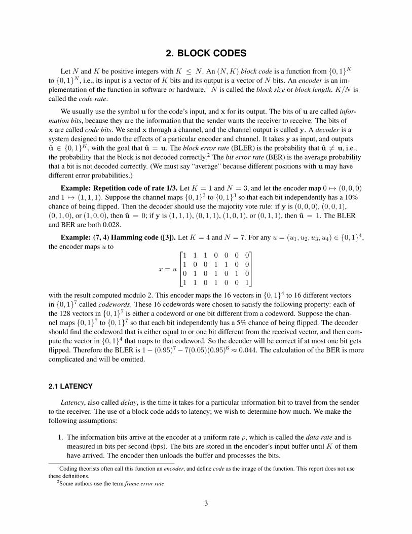
Example: (7, 4) Hamming code ([3]). Let K = 4 and N = 7. For any u = (u1, u2, u3, u4) ∈ {0, 1}4,the encoder maps u to
x = u
1 1 1 0 0 0 01 0 0 1 1 0 00 1 0 1 0 1 01 1 0 1 0 0 1
with the result computed modulo 2. This encoder maps the 16 vectors in {0, 1}4 to 16 different vectorsin {0, 1}7 called codewords. These 16 codewords were chosen to satisfy the following property: each ofthe 128 vectors in {0, 1}7 is either a codeword or one bit different from a codeword. Suppose the chan-nel maps {0, 1}7 to {0, 1}7 so that each bit independently has a 5% chance of being flipped. The decodershould find the codeword that is either equal to or one bit different from the received vector, and then com-pute the vector in {0, 1}4 that maps to that codeword. So the decoder will be correct if at most one bit getsflipped. Therefore the BLER is 1− (0.95)7− 7(0.05)(0.95)6 ≈ 0.044. The calculation of the BER is morecomplicated and will be omitted.
2.1 LATENCY
Latency, also called delay, is the time it takes for a particular information bit to travel from the senderto the receiver. The use of a block code adds to latency; we wish to determine how much. We make thefollowing assumptions:
1. The information bits arrive at the encoder at a uniform rate ρ, which is called the data rate and ismeasured in bits per second (bps). The bits are stored in the encoder’s input buffer until K of themhave arrived. The encoder then unloads the buffer and processes the bits.
1Coding theorists often call this function an encoder, and define code as the image of the function. This report does not usethese definitions.
2Some authors use the term frame error rate.
3

2. After the encoder has processed the bits for time Te, the N output bits are available in the encoder’soutput buffer. They leave the output buffer at a uniform rate N
K ρ.
3. The decoder does the same in reverse: the N -bit input buffer is filled at rate NK ρ, the decoder pro-
cesses the block in time Td, and the K-bit output buffer is emptied at rate ρ.
4. The encoder can only process one block at a time. It must be fast enough that when the last bit ofblock n arrives, it must be done encoding block n−1 so that it can immediately start encoding blockn; otherwise some of the bits of block n will be overwritten by bits of block n + 1. The same istrue of the decoder. This assumption puts a limit on the data rate at which a particular encoder anddecoder may be used.
The time to fill either input buffer or empty either output buffer is K/ρ. If block n begins arriving at theencoder at time t, then it finishes arriving at time t+K/ρ, and begins leaving at time t+K/ρ+Te. So thelatency added by the encoder is K/ρ+Te. Similarly, the latency added by the decoder is K/ρ+Td. By thelast assumption, Td and Te are both ≤ K/ρ, so the total latency added is between 2K/ρ and 4K/ρ.
For example, suppose K = 1024, Te = 10−5 s, and Td = 10−4 s. If the data rate is 150 bps, thenthe coding adds 13.7 s of latency, which is unacceptable for many purposes. In contrast, if the data rateis 1 megabit per second (Mbps), then the coding adds 2.16 milliseconds (ms) of latency, which might beinsignificant compared to other delays in the system. (For example, if the signal is relayed by a geosyn-chronous satellite, the propagation delay is about 250 ms.) The maximum possible data rate for this de-coder is K/Td = 10.24 Mbps.
4
3. INFORMATION THEORY
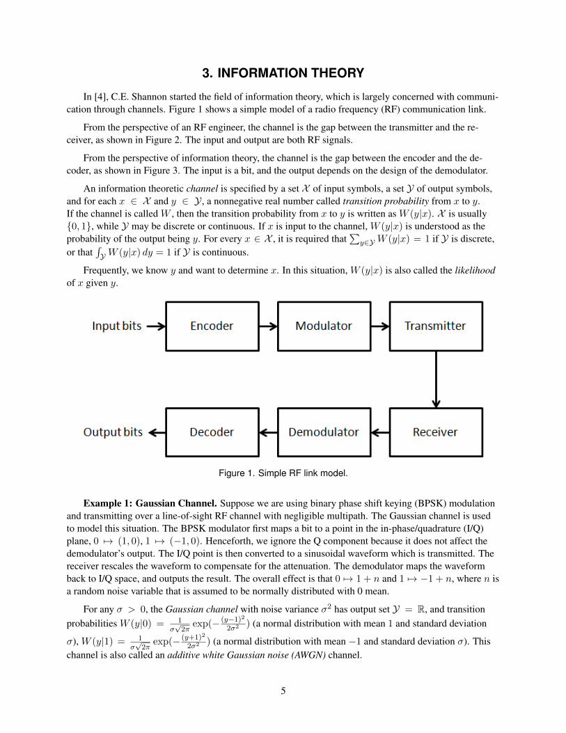
In [4], C.E. Shannon started the field of information theory, which is largely concerned with communi-cation through channels. Figure 1 shows a simple model of a radio frequency (RF) communication link.
From the perspective of an RF engineer, the channel is the gap between the transmitter and the re-ceiver, as shown in Figure 2. The input and output are both RF signals.
From the perspective of information theory, the channel is the gap between the encoder and the de-coder, as shown in Figure 3. The input is a bit, and the output depends on the design of the demodulator.
An information theoretic channel is specified by a set X of input symbols, a set Y of output symbols,and for each x ∈ X and y ∈ Y , a nonnegative real number called transition probability from x to y.If the channel is called W , then the transition probability from x to y is written as W (y|x). X is usually{0, 1}, while Y may be discrete or continuous. If x is input to the channel, W (y|x) is understood as theprobability of the output being y. For every x ∈ X , it is required that
∑y∈YW (y|x) = 1 if Y is discrete,
or that∫YW (y|x) dy = 1 if Y is continuous.
Frequently, we know y and want to determine x. In this situation, W (y|x) is also called the likelihoodof x given y.
Figure 1. Simple RF link model.
Example 1: Gaussian Channel. Suppose we are using binary phase shift keying (BPSK) modulationand transmitting over a line-of-sight RF channel with negligible multipath. The Gaussian channel is usedto model this situation. The BPSK modulator first maps a bit to a point in the in-phase/quadrature (I/Q)plane, 0 7→ (1, 0), 1 7→ (−1, 0). Henceforth, we ignore the Q component because it does not affect thedemodulator’s output. The I/Q point is then converted to a sinusoidal waveform which is transmitted. Thereceiver rescales the waveform to compensate for the attenuation. The demodulator maps the waveformback to I/Q space, and outputs the result. The overall effect is that 0 7→ 1 + n and 1 7→ −1 + n, where n isa random noise variable that is assumed to be normally distributed with 0 mean.
For any σ > 0, the Gaussian channel with noise variance σ2 has output set Y = R, and transitionprobabilities W (y|0) = 1
σ√
2πexp(− (y−1)2
2σ2 ) (a normal distribution with mean 1 and standard deviation
σ), W (y|1) = 1σ√
2πexp(− (y+1)2
2σ2 ) (a normal distribution with mean −1 and standard deviation σ). Thischannel is also called an additive white Gaussian noise (AWGN) channel.
5
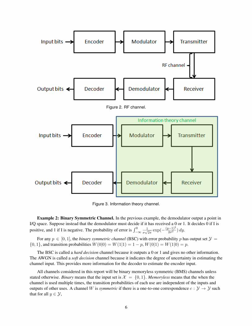
Figure 2. RF channel.
Figure 3. Information theory channel.
Example 2: Binary Symmetric Channel. In the previous example, the demodulator output a point inI/Q space. Suppose instead that the demodulator must decide if it has received a 0 or 1. It decides 0 if I ispositive, and 1 if I is negative. The probability of error is
∫ 0−∞
1σ√
2πexp(− (y−1)2
2σ2 ) dy.
For any p ∈ [0, 1], the binary symmetric channel (BSC) with error probability p has output set Y ={0, 1}, and transition probabilities W (0|0) = W (1|1) = 1− p, W (0|1) = W (1|0) = p.
The BSC is called a hard decision channel because it outputs a 0 or 1 and gives no other information.The AWGN is called a soft decision channel because it indicates the degree of uncertainty in estimating thechannel input. This provides more information for the decoder to estimate the encoder input.
All channels considered in this report will be binary memoryless symmetric (BMS) channels unlessstated otherwise. Binary means that the input set is X = {0, 1}. Memoryless means that the when thechannel is used multiple times, the transition probabilities of each use are independent of the inputs andoutputs of other uses. A channel W is symmetric if there is a one-to-one correspondence c : Y → Y suchthat for all y ∈ Y ,
6
1. c(c(y)) = y;
2. W (y|0) = W (c(y)|1);
3. W (y|1) = W (c(y)|0).
c(y) is usually written y. For the BSC, 0 = 1 and 1 = 0. For the AWGN channel, y = −y.
3.1 CHANNEL CAPACITY
Shannon showed how to compute the capacity C(W ) of a channel W , which is the highest rate atwhich information can be sent through the channel with arbitrarily low BER. Formally, he proved that forany rational number r < C(W ), and every ε > 0, there is an code with rate r and a corresponding decoderthat can decode the channel output with BER < ε, but this is not possible for any r > C(W ). Shannon’sproof did not show how to explicitly construct such a code. Furthermore, the decoder in his proof is a max-imum likelihood decoder. For any u ∈ {0, 1}K , the likelihood of u is the probability that this u wouldproduce the given y. The maximum likelihood decoder computes the likelihood of all 2K possible u’s, andoutputs the one with the maximum likelihood. This requires O(2K) steps, which is not practical except forvery small values of K.
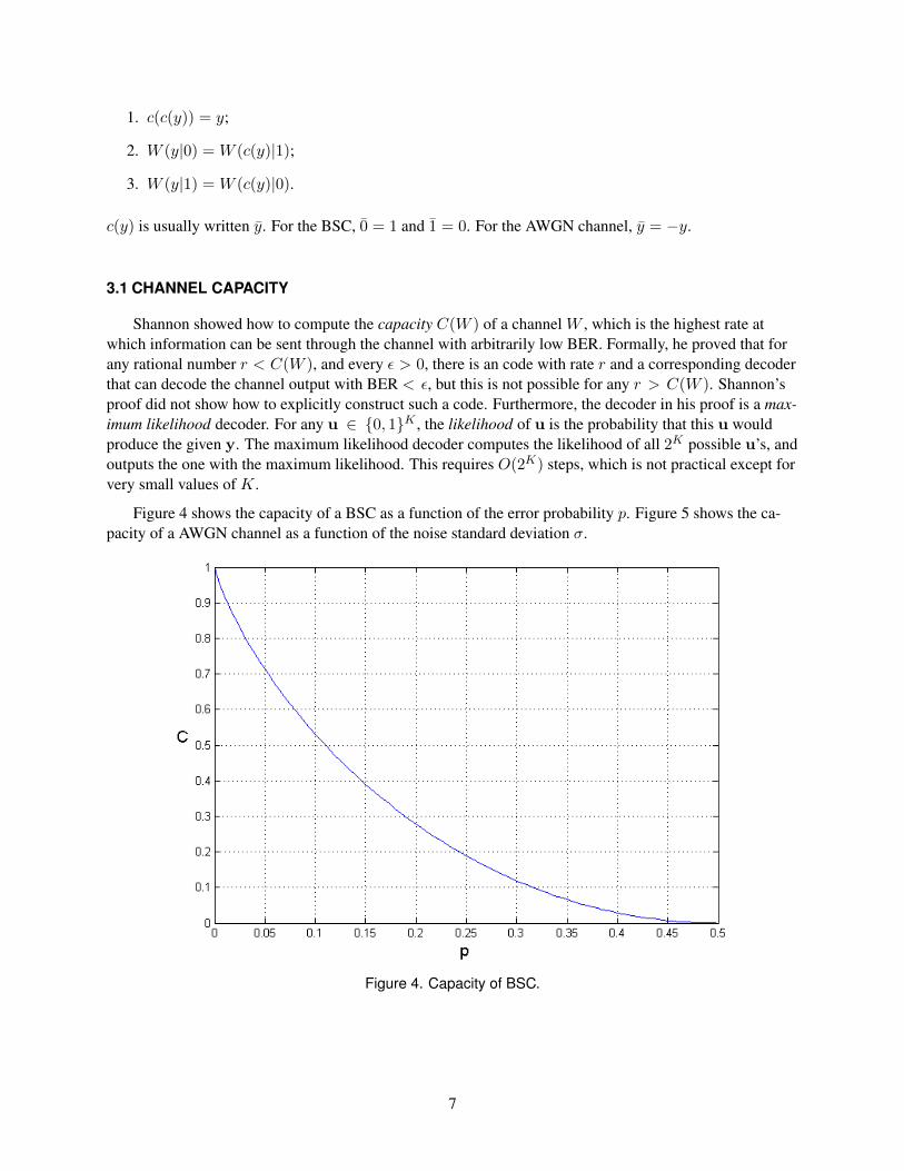
Figure 4 shows the capacity of a BSC as a function of the error probability p. Figure 5 shows the ca-pacity of a AWGN channel as a function of the noise standard deviation σ.
Figure 4. Capacity of BSC.
7

Figure 5. Capacity of AWGN channel.
8
4. INTRODUCTION TO POLAR CODES
Polar codes were introduced by E. Arikan in [1]. This paper showed how to construct polar encodersand decoders for any block length N that is a power of 2, and any K ≤ N . These encoders and decodersare relatively efficient, requiring O(N logN) instructions, as opposed to O(2K) for a maximum likeli-hood decoder. They were the first efficient encoders and decoders proven to achieve the capacity of anyBMS channel. This is not as useful as it sounds. Achieving the capacity of a channel W does not mean ex-hibiting a code with rate C(W ). It means exhibiting an infinite sequence of codes such that as N goes toinfinity, the code rate converges to C(W ) and BER converges to 0. So to produce a polar code with a ratevery close to the channel capacity, we may need a block length that is too large to use.
Reference [5] states that polar codes by themselves have underperformed state-of-the-art codes of sim-ilar block lengths and code rates. This may not be the most relevant comparison because the efficiencyof polar codes may make them feasible at larger block lengths than other codes; on the other hand, largerblock lengths may cause unacceptable latency.
Several authors have achieved better results by combining polar codes with other codes, for example,[5–7]. In particular, I. Tal and A. Vardy [5] combined a polar code with a cyclic redundancy check (CRC)and found that the resulting code of length 2048 outperformed the length 2304 LDPC code used in theWiMax standard. In [8, 9], K. Nui, K. Chen, and J.R. Lin combined polar codes of length 512, 1024, and2048 with a CRC. They also combined this CRC with turbo codes of the same lengths, and found that thepolar codes outperformed the turbo codes. However, [8, 9] compared BLERs and did not give any BERresults.
Polar codes can also be used for source coding (i.e., compression), but this use will not be discussed inthis report.
9

5. POLAR ENCODER
An (N,K) polar code is a block code with K inputs and N outputs. However, we will begin by in-troducing a function GN that has N bit inputs, which are numbered from 1 to N , and N bit outputs, alsonumbered from 1 to N . The input to GN is a row vector called u = (u1, u2, . . . , uN ), where ui is the bitthat goes into input i.3 This disagrees with the notation in Section 2, where we stated that u is a vector oflength K. The output of GN is a row vector of length N called x = (x1, x2, . . . , xN ).
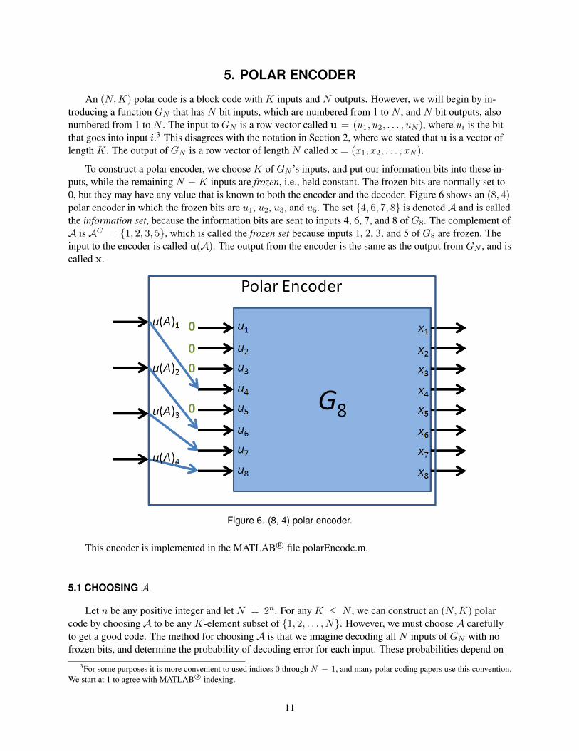
To construct a polar encoder, we choose K of GN ’s inputs, and put our information bits into these in-puts, while the remaining N − K inputs are frozen, i.e., held constant. The frozen bits are normally set to0, but they may have any value that is known to both the encoder and the decoder. Figure 6 shows an (8, 4)polar encoder in which the frozen bits are u1, u2, u3, and u5. The set {4, 6, 7, 8} is denoted A and is calledthe information set, because the information bits are sent to inputs 4, 6, 7, and 8 of G8. The complement ofA is AC = {1, 2, 3, 5}, which is called the frozen set because inputs 1, 2, 3, and 5 of G8 are frozen. Theinput to the encoder is called u(A). The output from the encoder is the same as the output from GN , and iscalled x.
Figure 6. (8, 4) polar encoder.
This encoder is implemented in the MATLAB R© file polarEncode.m.
5.1 CHOOSING A
Let n be any positive integer and let N = 2n. For any K ≤ N , we can construct an (N,K) polarcode by choosing A to be any K-element subset of {1, 2, . . . , N}. However, we must choose A carefullyto get a good code. The method for choosing A is that we imagine decoding all N inputs of GN with nofrozen bits, and determine the probability of decoding error for each input. These probabilities depend on
3For some purposes it is more convenient to used indices 0 through N − 1, and many polar coding papers use this convention.We start at 1 to agree with MATLAB R© indexing.
11
the channel W . We optimize the polar code for W by choosing A as the set of inputs with the lowest errorprobabilities.
5.2 STRUCTURE OF GN
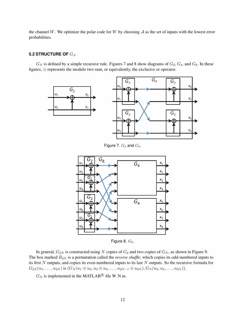
GN is defined by a simple recursive rule. Figures 7 and 8 show diagrams of G2, G4, and G8. In thesefigures, ⊕ represents the modulo two sum, or equivalently, the exclusive or operator.
Figure 7. G2 and G4.
Figure 8. G8.
In general, G2N is constructed using N copies of G2 and two copies of GN , as shown in Figure 9.The box marked R2N is a permutation called the reverse shuffle, which copies its odd-numbered inputs toits first N outputs, and copies its even-numbered inputs to its last N outputs. So the recursive formula forG2N (u1, . . . , u2N ) is (GN (u1 ⊕ u2, u3 ⊕ u4, . . . , u2N−1 ⊕ u2N ), GN (u2, u4, . . . , u2N )).
GN is implemented in the MATLAB R© file W N.m.
12
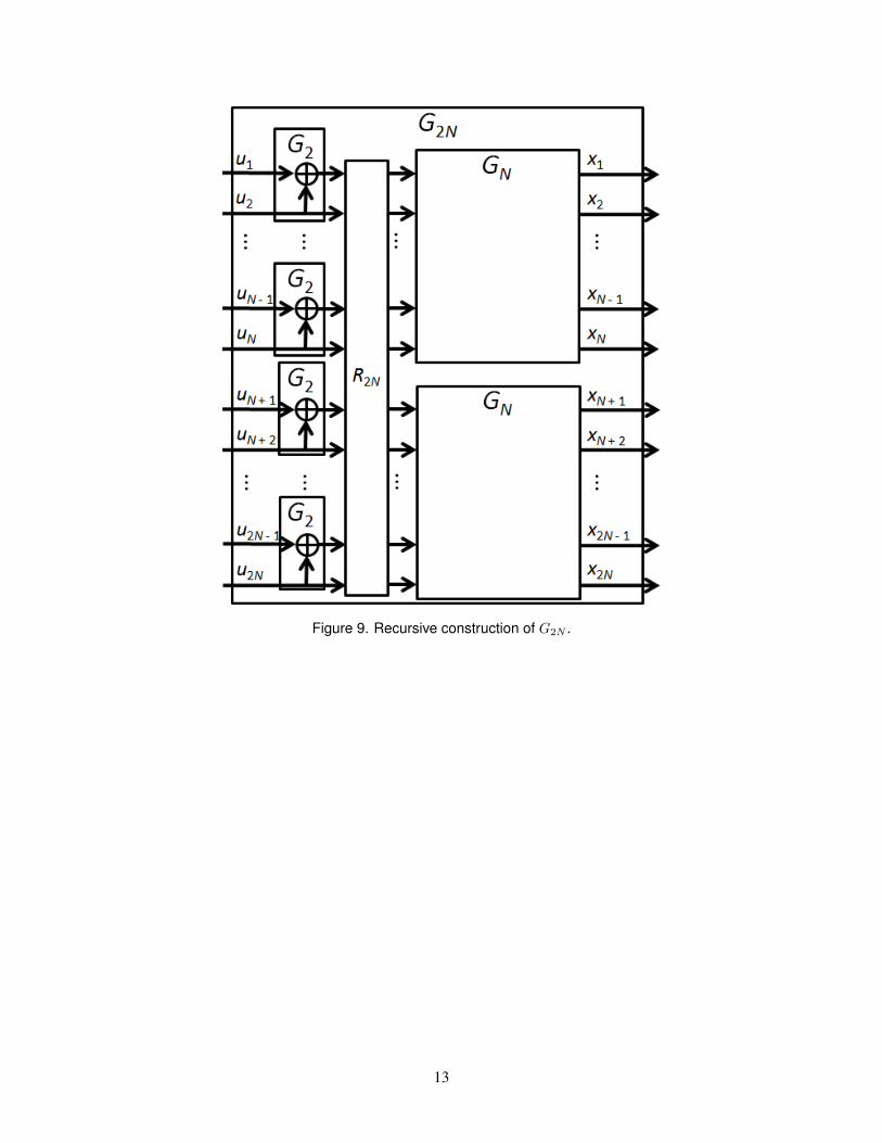
Figure 9. Recursive construction of G2N .
13

6. POLAR DECODER
The decoder described in [1] is called a successive cancellation (SC) decoder. It makes bit decisionsone at a time. When decoding the ith bit, the data it uses are the channel output y, and the previous bitdecisions u1 through ui−1, which it assumes are correct. It uses the following rules:
• If the ith input is frozen, then ui is known, so set ui = ui.
• If the ith input is not frozen, then choose ui to be the bit value that would have a higher probabilityto produce the channel output y. This probability is denoted W (i)
N (y1, . . . , yN , u1, . . . , ui−1|ui).
To compute W (i)N (y1, . . . , yN , u1, . . . , ui−1|ui = 0), choose bit values ui+1 through uN , and let
x = GN (u1, . . . , ui−1, 0, ui+1, . . . , uN ),
i.e., the encoder output when (u1, . . . , ui−1, 0, ui+1, . . . , uN ) is the input to GN . The probability of send-ing x through the channel and receiving y is
∏Ni=1W (yi|xi). We average this value over all 2N−i choices
of ui+1 through uN , and the result is W (i)N (y1, . . . , yN , u1, . . . , ui−1|ui = 0).
We then compute W (i)N (y1, . . . , yN , u1, . . . , ui−1|ui = 1) the same way. If
W(i)N (y1, . . . , yN , u1, . . . , ui−1|ui = 0) ≥W (i)
N (y1, . . . , yN , u1, . . . , ui−1|ui = 1), (1)
we choose ui = 0; otherwise, we choose ui = 1. 4
If we applied this rule directly, the complexity of the decoder would be Θ(2N ). Fortunately, [1] de-scribes a recursive method that reduces the complexity to Θ(N logN).
After the decoder is done computing u1 through uN , it outputs u(A), the estimates of the K non-frozen inputs.
6.1 LENGTH 2 DECODER
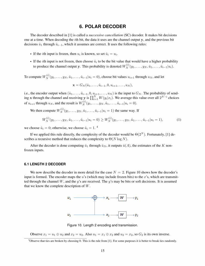
We now describe the decoder in more detail for the case N = 2. Figure 10 shows how the decoder’sinput is formed. The encoder maps the u’s (which may include frozen bits) to the x’s, which are transmit-ted through the channel W , and the y’s are received. The y’s may be bits or soft decisions. It is assumedthat we know the complete description of W .
Figure 10. Length 2 encoding and transmission.
Observe x1 = u1 ⊕ u2 and x2 = u2. Also u1 = x1 ⊕ x2 and u2 = x2, so G2 is its own inverse.4Observe that ties are broken by choosing 0. This is the rule from [1]. For some purposes it is better to break ties randomly.
15
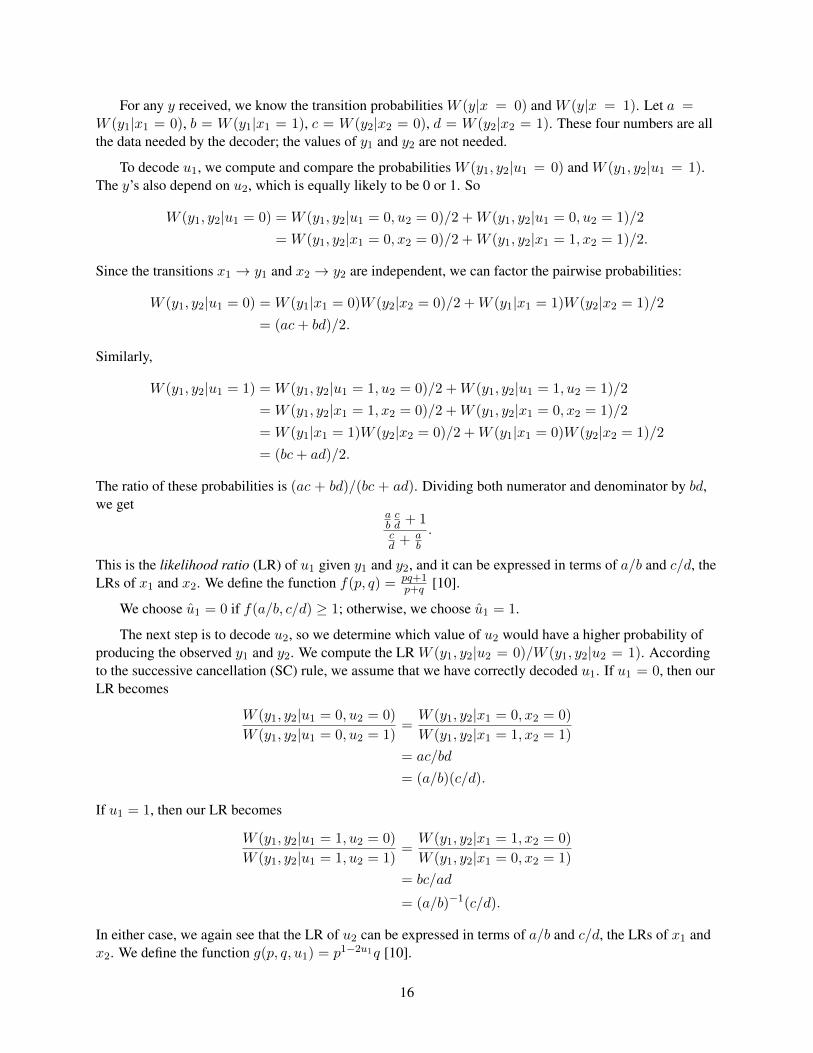
For any y received, we know the transition probabilities W (y|x = 0) and W (y|x = 1). Let a =W (y1|x1 = 0), b = W (y1|x1 = 1), c = W (y2|x2 = 0), d = W (y2|x2 = 1). These four numbers are allthe data needed by the decoder; the values of y1 and y2 are not needed.
To decode u1, we compute and compare the probabilities W (y1, y2|u1 = 0) and W (y1, y2|u1 = 1).The y’s also depend on u2, which is equally likely to be 0 or 1. So
W (y1, y2|u1 = 0) = W (y1, y2|u1 = 0, u2 = 0)/2 +W (y1, y2|u1 = 0, u2 = 1)/2
= W (y1, y2|x1 = 0, x2 = 0)/2 +W (y1, y2|x1 = 1, x2 = 1)/2.
Since the transitions x1 → y1 and x2 → y2 are independent, we can factor the pairwise probabilities:
W (y1, y2|u1 = 0) = W (y1|x1 = 0)W (y2|x2 = 0)/2 +W (y1|x1 = 1)W (y2|x2 = 1)/2
= (ac+ bd)/2.
Similarly,
W (y1, y2|u1 = 1) = W (y1, y2|u1 = 1, u2 = 0)/2 +W (y1, y2|u1 = 1, u2 = 1)/2
= W (y1, y2|x1 = 1, x2 = 0)/2 +W (y1, y2|x1 = 0, x2 = 1)/2
= W (y1|x1 = 1)W (y2|x2 = 0)/2 +W (y1|x1 = 0)W (y2|x2 = 1)/2
= (bc+ ad)/2.
The ratio of these probabilities is (ac + bd)/(bc + ad). Dividing both numerator and denominator by bd,we get
abcd + 1cd + a
b
.
This is the likelihood ratio (LR) of u1 given y1 and y2, and it can be expressed in terms of a/b and c/d, theLRs of x1 and x2. We define the function f(p, q) = pq+1
p+q [10].
We choose u1 = 0 if f(a/b, c/d) ≥ 1; otherwise, we choose u1 = 1.
The next step is to decode u2, so we determine which value of u2 would have a higher probability ofproducing the observed y1 and y2. We compute the LR W (y1, y2|u2 = 0)/W (y1, y2|u2 = 1). Accordingto the successive cancellation (SC) rule, we assume that we have correctly decoded u1. If u1 = 0, then ourLR becomes
W (y1, y2|u1 = 0, u2 = 0)
W (y1, y2|u1 = 0, u2 = 1)=W (y1, y2|x1 = 0, x2 = 0)
W (y1, y2|x1 = 1, x2 = 1)
= ac/bd
= (a/b)(c/d).
If u1 = 1, then our LR becomes
W (y1, y2|u1 = 1, u2 = 0)
W (y1, y2|u1 = 1, u2 = 1)=W (y1, y2|x1 = 1, x2 = 0)
W (y1, y2|x1 = 0, x2 = 1)
= bc/ad
= (a/b)−1(c/d).
In either case, we again see that the LR of u2 can be expressed in terms of a/b and c/d, the LRs of x1 andx2. We define the function g(p, q, u1) = p1−2u1q [10].
16

We choose u2 = 0 if g(a/b, c/d, u1) ≥ 1; otherwise we choose u2 = 1.
Therefore the decoder does not need all four values a, b, c, and d. Having LRs a/b and c/d is suffi-cient.
One may ask, if y2 is a soft estimate of x2, and x2 = u2, why don’t we use the same estimate for u2?If x2 is more likely to be 0 than 1 (or vice versa), then isn’t the same true for u2? Usually it is. An excep-tion can occur when the LR of u1 is < 1 (indicating u1 is more likely 1) but u1 is a frozen 0. This meansthat a bit got flipped in transmission. If y1 is a strong 0 and y2 is a weak 1, then y2 is more likely to be in-correct, so we conclude x2 = u2 = 0.
In the next section, estimates of x1 and x2 will also be necessary. These are computed x1 = u1 ⊕ u2
and x2 = u2.
6.2 EFFICIENT LENGTH N DECODER
The decoder needs the following inputs:
• The LRs of the N encoder outputs
• The set A ⊆ {1, . . . , N} of frozen indices
• u(AC), the known values of the frozen bits
In Figure 7, G4 has three columns that each contain four bit values: the input column, the output col-umn, and the middle column that has the bits u1 ⊕ u2, u2, u3 ⊕ u4, and u4. G4 also contains four copies ofG2: two on the left that transform the input bits to the middle bits, and two on the right that transform themiddle bits to the output bits. Similarly, in Figure 8, we can mentally fill in the missing details of the G4’s,and see that G8 has four columns that each contain eight bit values, and between these columns are threecolumns that each contain four copies of G2. In general, for N = 2n, GN has n + 1 columns that eachcontain N bit values, and n columns that each contain N/2 copies of G2.
The decoder works by following the structure of GN , repeating the procedure in Section 6.1 for eachof the nN/2 copies of G2. In this way, it retraces the encoder’s steps, and produces a LR and a bit estimatefor each of the (n+ 1)N bits in the encoder. The decoder has nN/2 elements that each represent one copyof G2. The connections between these elements parallel the connections in the decoder. LRs are input onthe right side of the decoder (representing the encoder output) and are computed from right to left. Bit esti-mates are first made at the left, and are computed from left to right.
For any bit b in the encoder, let L(b) be its LR, and let b be the decoder’s estimate. Each decoding ele-ment follows the steps listed below. In these steps we will use the symbols u1, u2, x1, and x2 for the inputsand outputs of a particular copy of G2, regardless of its place in GN . One element’s x1 may be anotherelement’s u1 or u2.
1. If this element is in the rightmost column, then L(x1) and L(x2) are included in the decoder’s input.Otherwise, wait until they are computed by elements in the next column to the right.
2. Set L(u1) = f(L(x1), L(x2)).
3. If this element is in the leftmost column, then set u1 using the decision rule: if this is a frozen bit,use the known value, otherwise set u1 = 0 if L(u1) ≥ 1, or u1 = 1 if L(u1) < 1. If this element isnot in the leftmost column, wait for u1 to be computed by an element in the next column to the left.
17
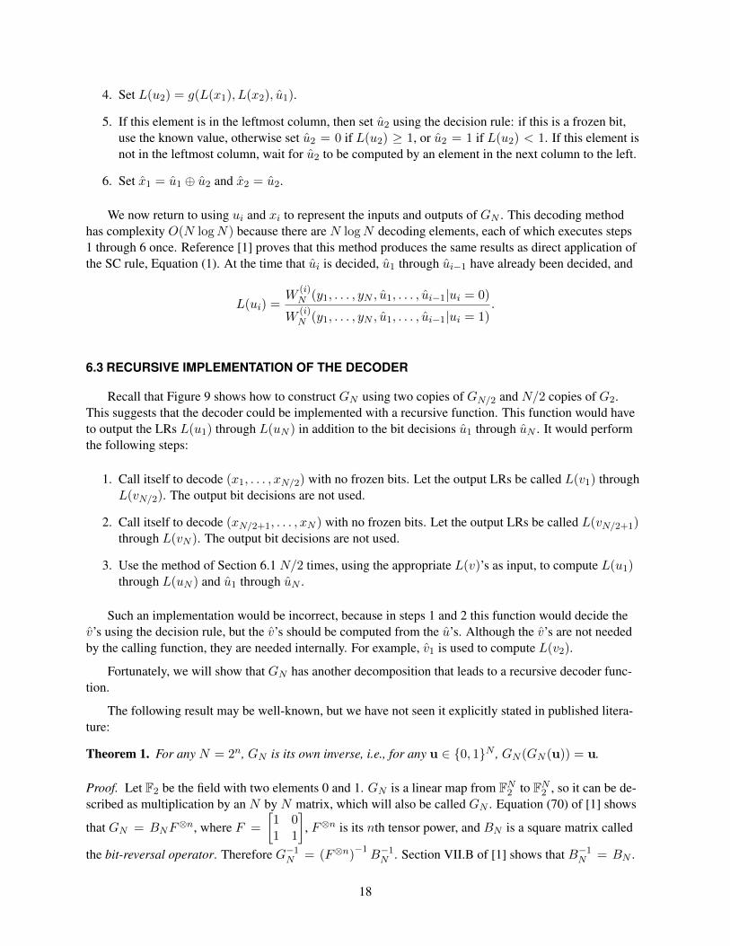
4. Set L(u2) = g(L(x1), L(x2), u1).
5. If this element is in the leftmost column, then set u2 using the decision rule: if this is a frozen bit,use the known value, otherwise set u2 = 0 if L(u2) ≥ 1, or u2 = 1 if L(u2) < 1. If this element isnot in the leftmost column, wait for u2 to be computed by an element in the next column to the left.
6. Set x1 = u1 ⊕ u2 and x2 = u2.
We now return to using ui and xi to represent the inputs and outputs of GN . This decoding methodhas complexity O(N logN) because there are N logN decoding elements, each of which executes steps1 through 6 once. Reference [1] proves that this method produces the same results as direct application ofthe SC rule, Equation (1). At the time that ui is decided, u1 through ui−1 have already been decided, and
L(ui) =W
(i)N (y1, . . . , yN , u1, . . . , ui−1|ui = 0)
W(i)N (y1, . . . , yN , u1, . . . , ui−1|ui = 1)
.
6.3 RECURSIVE IMPLEMENTATION OF THE DECODER
Recall that Figure 9 shows how to construct GN using two copies of GN/2 and N/2 copies of G2.This suggests that the decoder could be implemented with a recursive function. This function would haveto output the LRs L(u1) through L(uN ) in addition to the bit decisions u1 through uN . It would performthe following steps:
1. Call itself to decode (x1, . . . , xN/2) with no frozen bits. Let the output LRs be called L(v1) throughL(vN/2). The output bit decisions are not used.
2. Call itself to decode (xN/2+1, . . . , xN ) with no frozen bits. Let the output LRs be called L(vN/2+1)through L(vN ). The output bit decisions are not used.
3. Use the method of Section 6.1 N/2 times, using the appropriate L(v)’s as input, to compute L(u1)through L(uN ) and u1 through uN .
Such an implementation would be incorrect, because in steps 1 and 2 this function would decide thev’s using the decision rule, but the v’s should be computed from the u’s. Although the v’s are not neededby the calling function, they are needed internally. For example, v1 is used to compute L(v2).
Fortunately, we will show that GN has another decomposition that leads to a recursive decoder func-tion.
The following result may be well-known, but we have not seen it explicitly stated in published litera-ture:
Theorem 1. For any N = 2n, GN is its own inverse, i.e., for any u ∈ {0, 1}N , GN (GN (u)) = u.
Proof. Let F2 be the field with two elements 0 and 1. GN is a linear map from FN2 to FN2 , so it can be de-scribed as multiplication by an N by N matrix, which will also be called GN . Equation (70) of [1] shows
that GN = BNF⊗n, where F =
[1 01 1
], F⊗n is its nth tensor power, and BN is a square matrix called
the bit-reversal operator. Therefore G−1N = (F⊗n)
−1B−1N . Section VII.B of [1] shows that B−1
N = BN .
18

Also we see by direct computation that FF = I2. Using the tensor product identity (AC) ⊗ (BD) =(A⊗B)(C⊗D), we get that (F ⊗F )(F ⊗F ) = I2⊗ I2 = I4. By induction on n, we get F⊗nF⊗n = IN ,so (F⊗n)
−1= F⊗n. Combining these equations, we get G−1
N = F⊗nBN . Finally, Proposition 16 of [1]shows that F⊗nBN = GN .
We can make a diagram of G−1N by flipping Figure 9 horizontally, thus exchanging the roles of the in-
puts and outputs. Since G−1N = GN , this flipped diagram provides a second decomposition of GN , as
shown in Figure 11.
Figure 11. Second decomposition of GN .
(We have also replaced 2N with N , i.e., this figure shows GN in terms of GN/2, instead of G2N interms of GN .) When RN is flipped horizontally, it becomes R−1
N , which could be called the “shuffle”:
R−1N (v1, . . . , vN ) = (v1, vN/2+1, v2, vN/2+2, . . . , vN/2, vN ).
GN/2 and G2 also become their inverses, but by Theorem 1 this does not make a difference.
Now we can describe how to implement the decoder with a recursive function, using an algorithmbased on [11]. Recall that the inputs to the decoder are L(x1) through L(xN ), the set A of non-frozen in-
19

dices, and u(AC), the frozen bit values. The recursive function must output both u and x. The decoderexecutes these steps:
1. Split A into two pieces A1 = A ∩ {1, . . . , N/2} and A2 = A ∩ {N/2 + 1, . . . , N}, These arethe sets of non-frozen indices needed for the two recursive calls. Subtract N/2 from each element ofA2, because uN/2+1 through uN are called u1 through uN/2 within the second recursive call.
2. Split u(AC) into u(AC1 ) and u(AC2 ) in a similar way.
3. For 1 ≤ i ≤ N/2, compute L(w2i−1) = f(L(x2i−1), L(x2i)). This is step 2 from Section 6.2,repeated for each of the N/2 copies of G2 shown in Figure 11.
4. Call itself with inputs (L(w1), L(w3), . . . , L(wN−1)), A1, and u(AC1 ), producing outputs (u1, . . . , uN/2)and (v1, . . . , vN/2).
5. For 1 ≤ i ≤ N/2, compute L(w2i) = g(L(x2i−1), L(x2i), vi) (step 4 of Section 6.2).
6. Call itself with inputs (L(w2), L(w4), . . . , L(wN )), A2, and u(AC2 ), producing outputs (uN/2+1, . . . , uN )and (vN/2+1, . . . , vN ).
7. For 1 ≤ i ≤ N/2, compute x2i−1 = vi ⊕ vN/2+i and x2i = vN/2+i (step 6 of Section 6.2).
8. Return u and x.
This procedure has one minor shortcoming; it returns all N elements of u, instead of u(A), which is theestimate of the length K encoder input. In our MATLAB R© implementation, polarDecode.m version 3, thisproblem is handled by using a helper function to execute the above steps. The polarDecode functioncalls the helper function to obtain u (ignoring the x output) and then returns u(A).
6.4 NUMERICAL IMPLEMENTATION
Recall that f(x, y) = xy+1x+y is one of the functions we use to compute LRs. One difficulty in using this
function is that when we use it repeatedly, the LRs get closer to 1. The approach can be quite rapid: if δand ε are small, then f(1 + δ, 1 + ε) is approximately 1 + δε/2. Note that if neither x or y is exactly 1,then f(x, y) is not exactly 1, but when f(x, y) is computed in double-precision arithmetic the result couldbe 1, and this is likely to happen when decoding a large polar code. This is a problem because to make bitdecisions, we compare an LR to 1.
To avoid this problem, C. Leroux et al. [12] suggested computing the logarithms of the LRs (LLRs) in-stead of the LRs themselves. Then we make bit decisions by comparing LLRs to 0. This is better becausea double-precision LLR can be extremely close to 0. Such LLRs correspond to LRs extremely close to 1,which cannot be distinguished from 1 in double precision.
A hardware implementation of a decoder would usually compute with fixed-point numbers insteadof double precision. Fixed-point numbers cannot distinguish numbers near 0 as well as double precisionnumbers, but even so it is better to compute LLRs rather than LRs. The reason for this is that when decod-ing for a BMS channel, the LRs x and 1/x are equally likely to occur.
For example, if we are using LRs and are limited to 6 bits, we probably would choose to represent LRsfrom 1/8 to 8 in steps of 1/8 since 1/8 and 8 are equally likely. This means we have 56 different LRsgreater than 1 (probable zeroes), and only 7 less than 1 (probable ones). In contrast, we could represent
20

LLRs from −2 to 31/16 in steps of 1/16. These correspond to LRs from 0.135 to 6.94, roughly the samerange, with a good balance between probable zeros and probable ones, and slightly better resolution nearthe decision point.
Reference [12] showed that in decoding a (1024, 512) polar code, using 6-bit LLRs resulted in per-formance very close to floating point. did not specify The range of LLRs these 6 bits represented is notspecified in [12].
When we compute with LLRs, the formula for f(x, y) becomes
log
(exp(x) exp(y) + 1
exp(x) + exp(y)
).
If we use this formula as written when either x or y is near 0, it causes the same loss of precision that re-sults from computing with LRs near 1. Reference [10] gives the equivalent formula
f(x, y) = 2 tanh−1(
tanh(x
2
)tanh
(y2
)),
which is accurate near 0. The function g(x, y, 0) becomes x + y, and g(x, y, 1) becomes y − x. Reference[10] points out that these functions were already used for belief propagation decoding of LDPC codes. f isoften called the box operator, and is often replaced by an approximate formula sign(x) sign(y) min(|x|, |y|).Reference [12] showed that this approximation caused negligible performance degradation for N = 1024,and about 0.1 decibels (dB) performance degradation for N = 214.
Version 3 of polarDecode.m provides options to approximate the box operator and to compute in fixed-point. These features were removed in version 4 for ease of use.
6.5 FEASIBLE BLOCK SIZES
Because [1] proved that better results can be achieved with large block sizes, it is of interest to deter-mine what block sizes can be implemented in practice.
Many papers, including [12–17] have proposed implementing polar coding in field programmable gatearrays (FPGAs) or application-specific integrated circuits (ASICs). Such designs can be much faster thansoftware implementations, enabling large block sizes at high data rates.
Reference [14] describes an FPGA implementation that scales up to N = 221. The limiting factor isthe amount of SRAM on the chip. Table VIII of [14] shows that block size 221 requires 39,853,440 bits,which is available on an Altera Stratix R© V 5SGXMB6R3F43I4 FPGA. The maximum data rate of thisdesign is ρ = 33 K
221Mpbs. Therefore, it decodes a block in Td = 221
33·106s = 64 ms. With a code rate of
1/2 and data rate of 10 Mbps, the total latency is about 270 ms.
Using the formula from [14], but different numbers of quantization bits (Qc = 6, Q = 4), we foundthat block size 222 requires 48,236,032 bits of SRAM, which is available on some Stratix R© V models. De-coding a block requires 12.3 million clock cycles. We cannot predict Td because the clock speed must bedetermined through FPGA synthesis.
The largest block size we have found in the polar codes literature was 223, in [18]. This code size wassimulated in software. The throughput was not specified.
21


7. PERFORMANCE ANALYSIS
7.1 VIRTUAL CHANNELS
Figure 3 showed that an information-theoretic channel can encompass modulation and demodulationin addition to RF propagation. We can go further, and include the encoder and decoder in the channel, orparts of them, as shown in Figure 12. This figure shows a channel whose input is ui for some i between 1and N , and its output is the information that the decoder uses to determine ui, namely y and u1 throughui−1. (The set of possible output symbols is YN × {0, 1}i−1.) This channel represents how difficult it is tocorrectly decode ui.
Reference [1] describes an genie-aided decoder that has access to the true values of u1 through ui−1,but not ui, at the time it decides ui. The genie-aided decoder uses u1 through ui−1 the same way the realdecoder uses u1 through ui−1. The genie-aided decoder is easier to analyze than the real decoder, and ithas a very useful property:
Figure 12. Virtual channel.
Proposition 2. The genie-aided decoder will decode a block correctly if and only if the real decoder does.
Proof. If either decoder makes a mistake, let ui be the first bit that either decoder decodes incorrectly.Since the real decoder did not make a mistake before the ith bit, we have uj = uj for 1 ≤ j < i. Soboth decoders use the same input to decode ui, so they produce the same answer.
Therefore, by analyzing the genie-aided decoder, we can prove results about the BLER of the real de-coder.
For 1 ≤ i ≤ N , the virtual channel W (i)N is constructed from a channel W , a length N polar encoder,
and a length N SC polar decoder. It has input ui, and output (y, u1, . . . , ui−1). (Again, the set of possibleoutput symbols is YN × {0, 1}i−1.) This channel represents how difficult it is for the genie-aided decoderto correctly decode ui.
A virtual channel can be represented by an array with two rows, corresponding to the inputs 0 and 1,and one column for each output symbol. The entries in the array are the transition probabilities, and bydefinition each row must sum to 1. For example, if the outputs of W are Y = {1, 2, 3, 4, 5, 6, 7, 8}, thenW
(3)4 has 8422 = 16384 different output symbols ranging from (1, 1, 1, 1, 0, 0) to (8, 8, 8, 8, 1, 1).
23
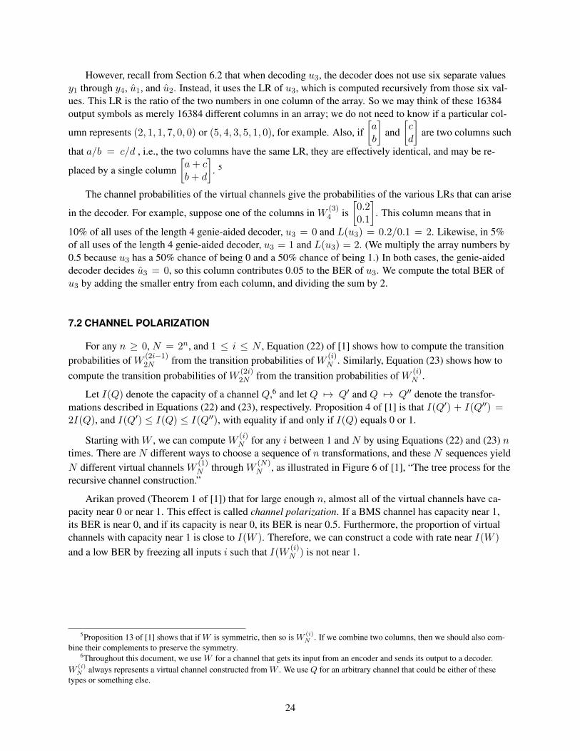
However, recall from Section 6.2 that when decoding u3, the decoder does not use six separate valuesy1 through y4, u1, and u2. Instead, it uses the LR of u3, which is computed recursively from those six val-ues. This LR is the ratio of the two numbers in one column of the array. So we may think of these 16384output symbols as merely 16384 different columns in an array; we do not need to know if a particular col-
umn represents (2, 1, 1, 7, 0, 0) or (5, 4, 3, 5, 1, 0), for example. Also, if[ab
]and
[cd
]are two columns such
that a/b = c/d , i.e., the two columns have the same LR, they are effectively identical, and may be re-
placed by a single column[a+ cb+ d
]. 5
The channel probabilities of the virtual channels give the probabilities of the various LRs that can arise
in the decoder. For example, suppose one of the columns in W (3)4 is
[0.20.1
]. This column means that in
10% of all uses of the length 4 genie-aided decoder, u3 = 0 and L(u3) = 0.2/0.1 = 2. Likewise, in 5%of all uses of the length 4 genie-aided decoder, u3 = 1 and L(u3) = 2. (We multiply the array numbers by0.5 because u3 has a 50% chance of being 0 and a 50% chance of being 1.) In both cases, the genie-aideddecoder decides u3 = 0, so this column contributes 0.05 to the BER of u3. We compute the total BER ofu3 by adding the smaller entry from each column, and dividing the sum by 2.
7.2 CHANNEL POLARIZATION
For any n ≥ 0, N = 2n, and 1 ≤ i ≤ N , Equation (22) of [1] shows how to compute the transitionprobabilities of W (2i−1)
2N from the transition probabilities of W (i)N . Similarly, Equation (23) shows how to
compute the transition probabilities of W (2i)2N from the transition probabilities of W (i)
N .
Let I(Q) denote the capacity of a channel Q,6 and let Q 7→ Q′ and Q 7→ Q′′ denote the transfor-mations described in Equations (22) and (23), respectively. Proposition 4 of [1] is that I(Q′) + I(Q′′) =2I(Q), and I(Q′) ≤ I(Q) ≤ I(Q′′), with equality if and only if I(Q) equals 0 or 1.
Starting with W , we can compute W (i)N for any i between 1 and N by using Equations (22) and (23) n
times. There are N different ways to choose a sequence of n transformations, and these N sequences yieldN different virtual channels W (1)
N through W (N)N , as illustrated in Figure 6 of [1], “The tree process for the
recursive channel construction.”
Arikan proved (Theorem 1 of [1]) that for large enough n, almost all of the virtual channels have ca-pacity near 0 or near 1. This effect is called channel polarization. If a BMS channel has capacity near 1,its BER is near 0, and if its capacity is near 0, its BER is near 0.5. Furthermore, the proportion of virtualchannels with capacity near 1 is close to I(W ). Therefore, we can construct a code with rate near I(W )
and a low BER by freezing all inputs i such that I(W(i)N ) is not near 1.
5Proposition 13 of [1] shows that if W is symmetric, then so is W (i)N . If we combine two columns, then we should also com-
bine their complements to preserve the symmetry.6Throughout this document, we use W for a channel that gets its input from an encoder and sends its output to a decoder.
W(i)N always represents a virtual channel constructed from W . We use Q for an arbitrary channel that could be either of these
types or something else.
24
8. CODE CONSTRUCTION
We construct an (N,K) polar code by choosing K elements of {1, . . . , N} to be the non-frozen in-dices. To get a good code for a particular BMS channel W , we must choose indices i such that I(W
(i)N ) is
near 1. However, computing I(W(i)N ) exactly is not feasible for even moderate code sizes, because if W
has a outputs, then W (i)N has aN2i−1 outputs. Various approaches have been proposed for estimating the
capacity or BER of W (i)N .
8.1 TAL/VARDY METHOD
We consider [19] by I. Tal and A. Vardy as the state of the art in code construction. Their methoduses a parameter µ. A larger µ means a better approximation but also longer running time. To constructa code of length N , the algorithm uses O(Nµ2 logµ) instructions. Reference [19] gives results for val-ues of µ ranging from 8 to 512. The method works by starting with the transition probabilities of W , andthen constructing virtual channels following the tree process shown in Figure 6 of [1]. Reference [19] usesQ 7→ Q�Q and Q 7→ Q~Q for the channel transformations described in Equations (22) and (23) of [1].
Whenever a channel is constructed with > µ outputs, it is replaced by a similar channel with µ out-puts. At each leaf of the tree, we produce a channel Qi that is similar to W (i)
N , and we compute the BER ofQi to estimate the BER of W (i)
N .
One might ask how a channel with a huge number of outputs could be similar to a channel with a smallnumber of outputs. The answer is that the decoder only cares about the LR of each output. If we havemany symbols with approximately equal LRs, we can combine them to one symbol whose LR is withinthe range of those LRs, and this change has very little effect on the channel’s BER.
Reference [19] presents two methods to reduce the number of channel outputs to µ. The first methodis called “degrading merge”. It is used in “Algorithm A”, which guarantees that BER(Qi) ≥ BER(W
(i)N ).
The second method is called “upgrading merge”. It is used in “Algorithm B”, which guarantees that BER(Qi) ≤BER(W
(i)N ). Thus BER(W
(i)N ) is bounded between two values.7 If these values are far apart, it may be
worthwhile to rerun the algorithms with a larger µ to get a better estimate. Reference [19] gives examplesshowing that the bounds can be close together for large enough µ. It also presents “Algorithm D”, whichis the same as Algorithm A except that it computes an additional number Zi that is guaranteed to satisfyBER(Qi) ≥ Zi ≥ BER(W
(i)N ), giving an even better upper bound.
After running Algorithm A (resp. D), we construct an (N,K) polar code by letting A be the indices ofthe K smallest values of BER(Qi) (resp. Zi). The sum of these K values is an upper bound on the BLERof this code when used for channel W . K could be chosen in advance, or it could be chosen to achieve aparticular BLER bound.
8.1.1 Implementation
The file algorithmA.m is a MATLAB R© implementation of Algorithm A, and AlgorithmD.java is aJavaTM implementation of Algorithm D. We did not implement Algorithm B. Reference [19] also showshow to modify the degrading merge algorithm to convert a continuous channel to a similar discrete chan-nel. This algorithm assumes that we are able to compute integrals of the transition probabilities. We im-
7These guarantees depend on exactly implementing the operations described in the paper. If these operations are implementedwith double precision arithmetic, it is possible that accumulated rounding error could cause violation of the bounds.
25
plemented the continuous degrading merge for the specific case of an AWGN channel. The MATLAB R©
version is degradeAwgnToDiscrete.m, and the JavaTM version is a constructor in Channel.java.
The function algorithmA returns the capacity, BER, and Bhattacharyya parameter (see [1] for defi-nition) of each Qi. The user can then use other MATLAB R© functions to sort the BERs and choose A.
In the JavaTM implementation, the AlgorithmD class has a compute method that estimates BER(W(i)
2j)
for 1 ≤ j ≤ m and 1 ≤ i ≤ 2j . This class also has a computeAndSaveFixedRateCodes method.For each j this method sorts the 2j BER estimates, chooses A to construct a length 2j code of a specifiedrate, and computes the bound for this code’s BLER. Finally, this method creates a MATLAB R© script file.When this script is run in MATLAB R©, it creates one MAT-file for each code. The individual BER esti-mates are not available to MATLAB R©, but they are saved by serialization of the AlgorithmD object.
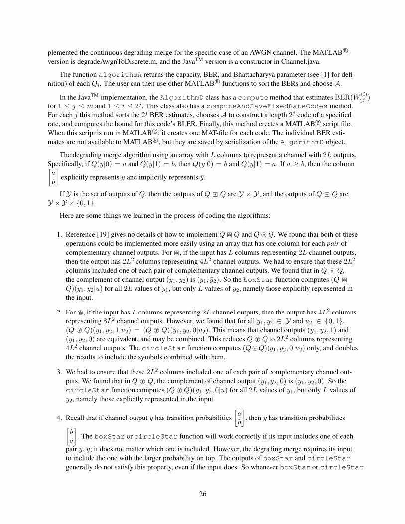
The degrading merge algorithm using an array with L columns to represent a channel with 2L outputs.Specifically, if Q(y|0) = a and Q(y|1) = b, then Q(y|0) = b and Q(y|1) = a. If a ≥ b, then the column[ab
]explicitly represents y and implicitly represents y.
If Y is the set of outputs of Q, then the outputs of Q � Q are Y × Y , and the outputs of Q � Q areY × Y × {0, 1}.
Here are some things we learned in the process of coding the algorithms:
1. Reference [19] gives no details of how to implement Q�Q and Q~Q. We found that both of theseoperations could be implemented more easily using an array that has one column for each pair ofcomplementary channel outputs. For �, if the input has L columns representing 2L channel outputs,then the output has 2L2 columns representing 4L2 channel outputs. We had to ensure that these 2L2
columns included one of each pair of complementary channel outputs. We found that in Q � Q,the complement of channel output (y1, y2) is (y1, y2). So the boxStar function computes (Q �Q)(y1, y2|u) for all 2L values of y1, but only L values of y2, namely those explicitly represented inthe input.
2. For ~, if the input has L columns representing 2L channel outputs, then the output has 4L2 columnsrepresenting 8L2 channel outputs. However, we found that for all y1, y2 ∈ Y and u2 ∈ {0, 1},(Q ~ Q)(y1, y2, 1|u2) = (Q ~ Q)(y1, y2, 0|u2). This means that channel outputs (y1, y2, 1) and(y1, y2, 0) are equivalent, and may be combined. This reduces Q ~ Q to 2L2 columns representing4L2 channel outputs. The circleStar function computes (Q~Q)(y1, y2, 0|u2) only, and doublesthe results to include the symbols combined with them.
3. We had to ensure that these 2L2 columns included one of each pair of complementary channel out-puts. We found that in Q ~ Q, the complement of channel output (y1, y2, 0) is (y1, y2, 0). So thecircleStar function computes (Q ~ Q)(y1, y2, 0|u) for all 2L values of y1, but only L values ofy2, namely those explicitly represented in the input.
4. Recall that if channel output y has transition probabilities[ab
], then y has transition probabilities[
ba
]. The boxStar or circleStar function will work correctly if its input includes one of each
pair y, y; it does not matter which one is included. However, the degrading merge requires its inputto include the one with the larger probability on top. The outputs of boxStar and circleStargenerally do not satisfy this property, even if the input does. So whenever boxStar or circleStar
26

outputs a column[ab
]with a < b, we replace this column with
[ba
], which represents the same pair
of complementary channel outputs.
5. The degrading merge works by combining channel outputs. Two columns[ab
]and
[cd
]with sim-
ilar LRs are replaced by a single column[a+ cb+ d
]. The degrading merge algorithm chooses which
columns to combine with the goal of minimizing the decrease in channel capacity.
One might ask, since we are ultimately interested in the BER of each virtual channel, why do weminimize the decrease in channel capacity, instead of minimizing the increase in BER? We discov-ered that combining columns of Q has no effect on the BER of Q, but it can increase the BER ofQ ~ Q and other channels that occur later in the tree. Reference [19] does not explain how to com-pute this effect, so it does not prove that this method of combining columns minimizes the increasein BER.
6. The degrading merge algorithm uses a heap data structure to determine which columns to combine.Reference [19] defines a heap as a data structure that associates keys to data, and supports four oper-ations:
• Insert: add a new key-value pair to the heap• GetMin: find the key-value pair with the minimum key in the heap• RemoveMin: remove the key-value pair with the minimum key in the heap• ValueUpdated: change the key of a key-value pair.
It states that getMin has running time O(1), and the other three operations have running time O(logL)where L is the size of the heap.
Such a structure is often called a min-heap, to distinguish it from a max-heap that supports getMaxand removeMax instead of getMin and removeMin.
Reference [19] refers to [20] for the heap implementation. However, the heap described in [20]does not support the valueUpdated operation. We searched the Internet for other heap implemen-tations, and found that max-heaps typically support increaseKey and min-heaps typically supportdecreaseKey, but we could not find an implementation that supports both. Fortunately, we found away to implement decreaseKey on a max-heap in O(logL) time.
8.1.2 Results
Table I of [19] shows some results of computing a (220, 445340) polar code for the channel BSC(p =0.11). It shows that using Algorithm A with µ = 8, the resulting BLER upper bound is 5.096030e-03.Using our implementation, we obtained 5.083668e-03, which is about 0.2% smaller.
Figure 2(b) of [19] shows some results of computing polar codes for the channel AWGN(σ2 = 0.1581).The code lengths are 210 and 220, and for each length the code rates range from 0.9 to 1. Reference [19]says “the value of µ did not exceed 512.” This figure is a graph with code rate on the horizontal axis, andthe base-10 logarithm of the BLER bound on the vertical axis.
We used AlgorithmD.java to repeat these calculations for the N = 210 case using µ = 512. Figure 13shows a graph of our results. The results appear to be very similar to Figure 2(b) of [19].
27

Figure 13. Reproducing a result from Tal and Vardy.
8.2 GAUSSIAN APPROXIMATION METHOD FOR AWGN CHANNELS
Recall from Section 7.1 that the transition probabilities of the virtual channels indicate the probabil-
ities of the various LRs that can arise in the decoder. A column[ab
]represents a probability (a + b)/2
that the LR equals a/b. The Tal/Vardy code construction method works by approximating the virtual chan-nel, using a channel with at most µ outputs. So the approximate LR distribution is described by a set of 2µnumbers, half of which may be omitted due to symmetry.
Several papers, including [6] and [21], have suggested that for an AWGN channel we can use a moreefficient method. If we describe the distribution of LLRs instead of LRs, we can use a much simpler ap-proximation: a Gaussian distribution. However, neither of these papers clearly explains why this methodworks. We found the explanation in [22] by D. Wu, Y. Li, and Y. Sun. However, their explanation requiresa correction.
Previously, we have used L to represent an LR, but in this section it will be an LLR. Let L(i)N denote
the LLR of W (i)N , i.e., the LLR of the ui computed by a genie-aided SC decoder. L(i)
N is a random variablethat depends on y and u1 through ui−1. L(2i−1)
N and L(2i)N are both computed recursively from two other
random variables that each have the distribution of L(i)N/2, using the functions f and g described in Section
6.4.
It is well known that when using optimal decoding of a linear block code with a BMS channel, theprobability of block error is the same regardless of which codeword was transmitted.8 The SC polar de-coder is not optimal, but Arikan proved something similar for SC decoding:
Theorem 3. (Corollary 1 of [1]) For 1 ≤ i ≤ N , the genie-aided decoder’s probability of incorrectlydecoding ui is the same regardless of which codeword is transmitted.
Therefore, we can assume for convenience that u and x are all zeroes. To see why this is helpful, referto the decoding procedure in Section 6.3. In the genie-aided decoder, it is the ui’s, not the ui’s, that propa-
8This assumes that ties are broken randomly. In an AWGN channel (or any continuous channel), the probability of an exact tieis 0, so we will ignore the possibility of ties in this section.
28

gate from left to right through the decoder. So when we compute L(w2i) = g(L(x2i−1), L(x2i), vi) in step5, vi is always 0, so g is always an addition, not a subtraction.
Now let W be an AWGN channel. Recall that its transition probabilities are W (y|0) = 1σ√
2πexp(− (y−1)2
2σ2 )
and W (y|1) = 1σ√
2πexp(− (y+1)2
2σ2 ). For any output y, the corresponding LLR is log(W (y|0)W (y|1)
), and since
we assume only 0’s are transmitted, the probability of this LLR occurring is W (y|0). We compute
L(y) = log
(W (y|0)
W (y|1)
)= log
1σ√
2πexp(− (y−1)2
2σ2 )
1σ√
2πexp(− (y+1)2
2σ2 )
= log
(exp
(−(y − 1)2
2σ2+
(y + 1)2
2σ2
))=−(y − 1)2 + (y + 1)2
2σ2=
2y
σ2.
Since y is a normally distributed variable with mean 1 and variance σ2, then L(y) = 2yσ2 is a normally
distributed variable with mean 2/σ2 and variance σ2(
2σ2
)2= 4/σ2. The variance is twice the mean. We
define a consistent normal density variable (CNDV) to be a normally distributed variable whose variance istwice its mean. Then L(y) is a CNDV.
Next, L(1)2 = f(L(y1), L(y2)), where L(y1) and L(y2) are both variables with the distribution of L(y).
According to the “GA principle,” when f is applied to two CNDVs, the result can be approximated by aCNDV. Therefore, L(1)
2 is an approximate CNDV. In addition, L(2)2 = g(L(y1), L(y2), 0) = L(y1) +L(y2).
It is well known that the sum of normal variables is a normal variable. The mean of the sum is the sum ofthe means, and the variance of the sum is the sum of the variances. So L(2)
2 has mean 4/σ2 and variance8/σ2, and is a CNDV. Applying these arguments repeatedly, we find that all of the virtual channels areapproximate CNDVs. However, it is not clear how much the approximation degrades when f is appliedrepeatedly.
Since each L(i)N is normally distributed with the variance equal to twice the mean, we can characterize
its distribution using the mean only, compared to µ parameters used in the Tal/Vardy method. We write thismean as E(L
(i)N ). We compute it recursively: E(L
(2i)N ) = 2E(L
(i)N/2), and E(L
(2i−1)N ) = ω
(E(L
(i)N/2)
),
where ω is defined byω(x) = φ−1
(1− (1− φ(x))2
)(2)
and φ is defined by
φ(x) = 1− 1√4πx
∫ ∞−∞
tanh(τ
2
)exp
[−(τ − x)2/(4x)
]dτ. (3)
Finally, BER(W(i)N ) = 1
2 erfc
(0.5
√E(L
(i)N )
).
8.2.1 Error in Wu, Li, and Sun
The procedure above computes an estimate of BER(W(i)N ), the probability of error of a genie-aided
decoder. However, [22] claims that this procedure computes P (Ci), defined as the conditional probabilityof a real (i.e., not genie-aided) SC decoder incorrectly decoding the ith bit, subject to the condition that allprevious bits are decoded correctly. The BLER is then computed as 1−
∏i∈A(1− P (Ci)).
At first glance, one might think that P (Ci) = BER(W(i)N ) because both are the probability of error
in a situation where the decoder has the correct value of all previous bits. However, BER(W(i)N ) considers
29
all possible values of y, but P (Ci) considers only values of y that would have caused all previous bits tobe decoded correctly. This imposes a selection bias on the channel noise. If several previous bits were alldecoded correctly, this probably means that not many bits were flipped in the channel, which means that uiis also more likely to be decoded correctly. Therefore, we expect P (Ci) < BER(W
(i)N ), although this is
not a proof.
P (Ci) is affected by frozen bits. If the ith bit is frozen then P (Ci) = 0, so assume the ith bit is notfrozen. If some of the first i − 1 bits are frozen, then this enlarges the set of vectors yN1 that will cause thefirst i − 1 bits to all be decoded correctly, so the bias is reduced. If the first i − 1 bits are all frozen, thenP (Ci) = BER(W
(i)N ).
For example, let N = 2, and let σ2 = 0.25. Using the algorithm of [22], we computed the esti-mates P (C1) = 0.04473 and P (C2) = 0.002363. We then ran 106 trials of encoding, transmission, andgenie-aided decoding with no frozen bits, producing the estimates P (C1) = BER(W
(1)2 ) = 0.044794,
BER(W(2)2 ) = 0.002304, and P (C2) = 5.4217 · 10−4. The corresponding 3-sigma confidence intervals are
(0.044173, 0.045415), (0.002160, 0.002448), and (4.5715 · 10−4, 5.9812 · 10−4). So the P (Ci)’s computedwith the algorithm agree with the simulation’s BER(W
(i)2 )’s.
If we had an efficient way to compute P (Ci), it would still be difficult to use this for code constructionbecause of the dependence on previous frozen bits.
8.2.2 Implementation
The file wuLiSun.m is our MATLAB R© implementation of the Gaussian approximation method.
The function φ is hard to compute because it requires integrating from −∞ to∞. Reference [22] usesan approximation:
φ(x) =
{exp(−0.4527x0.86 + 0.0218), 0 < x < 10,√
πx exp
(−x
4
) (1− 10
7x
)x ≥ 10.
(4)
Reference [22] then says “In practice, we can store samples of (4), and look up the result via a bi-searchmethod.” We took this to mean that the look-up table is used to compute φ−1. The look-up table containsφ(x) for many values of x. To compute φ−1(y), we find the value nearest y in the look-up table, and returnthe corresponding x. Reference [22] says nothing about how many values to include in the table or how tochoose them. We used 108 values of x, logarithmically spaced from 2−100 to 2100.
The file gaussianLlrXor.m is our MATLAB R© implementation of the function ω. We found that forvery small values of x, ω(x) > x. This cannot be correct because it would imply that Q � Q has a highercapacity than Q. Apparently, it indicates that the approximation of φ is not good for very small x. So wemodified gaussianLlrXor.m to return min(x, ω(x)). This is an improvement, but the results are still incor-rect for very small x.
8.2.3 Results
To compare the two code construction methods, we let W be AWGN(σ2 = 0.1581), N = 210, andused both methods to compute BER(W i
N ) for 1 ≤ i ≤ N . The function wuLiSun ran in 8 seconds,compared to 225 seconds for AlgorithmD.java. We also ran simulations of a genie-aided decoder in thischannel for about eight hours, a total of 479453 trials, to produce empirical estimates of BER(W i
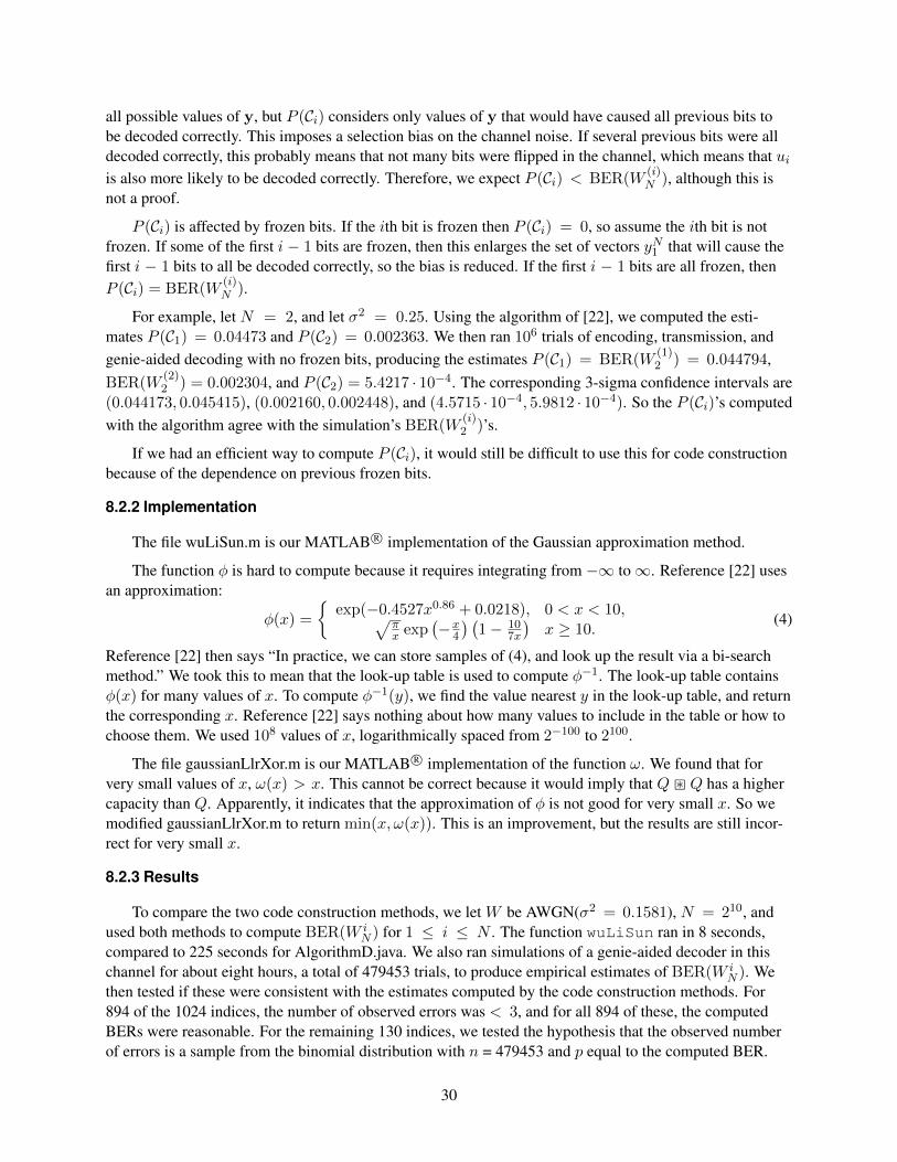
N ). Wethen tested if these were consistent with the estimates computed by the code construction methods. For894 of the 1024 indices, the number of observed errors was < 3, and for all 894 of these, the computedBERs were reasonable. For the remaining 130 indices, we tested the hypothesis that the observed numberof errors is a sample from the binomial distribution with n = 479453 and p equal to the computed BER.
30

We approximated the binomial distribution with a normal distribution with mean np and variance np(1 −p). The resulting Z-scores are in Figure 14.
Figure 14. Z scores.
The Tal/Vardy BER estimates appear very reasonable, as 64% are within one standard error of the em-pirical estimates, and 96% are within two standard errors, which is roughly what we expect. Only the one ,almost four standard errors above the mean, indicates a small inaccuracy in the method. In contrast, only47% of the Gaussian approximation estimates are within three standard errors, and 75% are within tenstandard errors. For seven of the indices (not shown), the empirical BER was more than 30 standard errorsabove the estimate.
On the other hand, if we are constructing a code with a predetermined rate, then this inaccuracy doesnot have a large effect. In Figure 15, the green line is the BLER bound computed with the Tal/Vardy method.The blue line is the BLER bound obtained by choosing A by the Gaussian approximation method, andthen using the BER estimates from the Tal/Vardy method.
The difference is never more than 10% except for lower values of K where the BLER bound is lessthan 10−6. The Gaussian approximation method may be useful if a code must be constructed quickly.However, for larger N or larger σ2, very small LLRs will arise more often, so the inaccuracy of this methodcould have a larger effect. It may be necessary to compute ω(x) more accurately for very small values ofx.
31
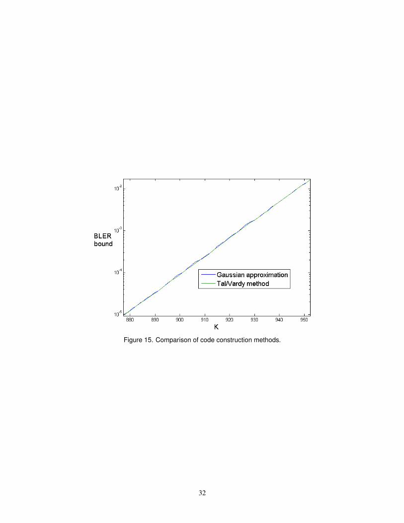
Figure 15. Comparison of code construction methods.
32
9. OTHER VERSIONS OF POLAR CODING
9.1 ENCODING WITH F⊗N
Recall that we defined the function GN as BNF⊗n. Section VII.C of [1] says “In an actual implemen-tation of polar codes, it may be preferable to use F⊗n in place of BNF⊗n as the encoder mapping in orderto simplify the implementation.”
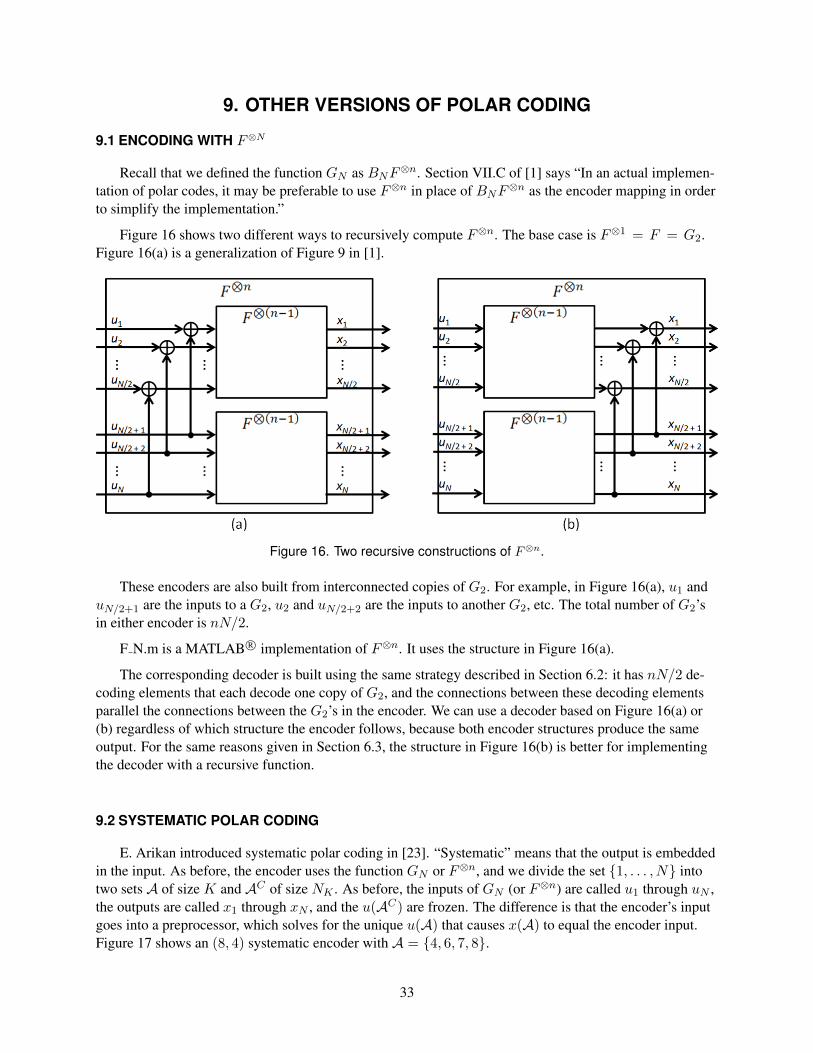
Figure 16 shows two different ways to recursively compute F⊗n. The base case is F⊗1 = F = G2.Figure 16(a) is a generalization of Figure 9 in [1].
Figure 16. Two recursive constructions of F⊗n.
These encoders are also built from interconnected copies of G2. For example, in Figure 16(a), u1 anduN/2+1 are the inputs to a G2, u2 and uN/2+2 are the inputs to another G2, etc. The total number of G2’sin either encoder is nN/2.
F N.m is a MATLAB R© implementation of F⊗n. It uses the structure in Figure 16(a).
The corresponding decoder is built using the same strategy described in Section 6.2: it has nN/2 de-coding elements that each decode one copy of G2, and the connections between these decoding elementsparallel the connections between the G2’s in the encoder. We can use a decoder based on Figure 16(a) or(b) regardless of which structure the encoder follows, because both encoder structures produce the sameoutput. For the same reasons given in Section 6.3, the structure in Figure 16(b) is better for implementingthe decoder with a recursive function.
9.2 SYSTEMATIC POLAR CODING
E. Arikan introduced systematic polar coding in [23]. “Systematic” means that the output is embeddedin the input. As before, the encoder uses the function GN or F⊗n, and we divide the set {1, . . . , N} intotwo sets A of size K and AC of size NK . As before, the inputs of GN (or F⊗n) are called u1 through uN ,the outputs are called x1 through xN , and the u(AC) are frozen. The difference is that the encoder’s inputgoes into a preprocessor, which solves for the unique u(A) that causes x(A) to equal the encoder input.Figure 17 shows an (8, 4) systematic encoder with A = {4, 6, 7, 8}.
33
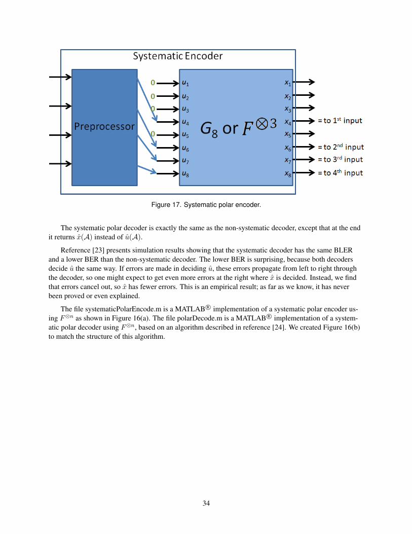
Figure 17. Systematic polar encoder.
The systematic polar decoder is exactly the same as the non-systematic decoder, except that at the endit returns x(A) instead of u(A).
Reference [23] presents simulation results showing that the systematic decoder has the same BLERand a lower BER than the non-systematic decoder. The lower BER is surprising, because both decodersdecide u the same way. If errors are made in deciding u, these errors propagate from left to right throughthe decoder, so one might expect to get even more errors at the right where x is decided. Instead, we findthat errors cancel out, so x has fewer errors. This is an empirical result; as far as we know, it has neverbeen proved or even explained.
The file systematicPolarEncode.m is a MATLAB R© implementation of a systematic polar encoder us-ing F⊗n as shown in Figure 16(a). The file polarDecode.m is a MATLAB R© implementation of a system-atic polar decoder using F⊗n, based on an algorithm described in reference [24]. We created Figure 16(b)to match the structure of this algorithm.
34
10. SIMULATIONS
10.1 MEASURES OF PERFORMANCE
Recall that in the Gaussian channel described in Section 3, the BPSK modulator outputs ±1, and thechannel output is ±1 + n where n is normally distributed with mean 0 and variance σ2. The quantity 1
2σ2
is often called the bit energy to noise power spectral density ratio (Eb/N0), and is usually expressed indecibels.
However, when FEC coding is used, Eb is redefined as the energy received per information bit, as op-posed to the symbol energy (Es), which is the amount of energy received in one use of the channel. Us-ing an (N,K) code, K bits of information are sent in N uses of the channel, so KEb = NEs. We haveEs/N0 = 1
2σ2 , and Eb/N0 = N2σ2K
. Es/N0 is a property of the channel, but Eb/N0 depends on the codeused with that channel.
In the polar codes literature, most reported simulation results are for Gaussian channels, and these re-sults are usually displayed with a graph called a waterfall plot. In these graphs, the vertical axis usuallyshows BER or BLER on a logarithmic scale, and the horizontal axis usually shows Eb/N0 in decibels.Figure 1 of [23] is a good example. This graph compares the performance of a systematic polar code withthe corresponding non-systematic code, so the graph has one line for each code. Each of these codes wastested in 13 different Gaussian channels, resulting in 13 points on each line.
10.2 ESTIMATING BER
We wrote the MATLAB R© function codeTest2 for simulating polar codes in Gaussian channels andestimating their BERs. It repeatedly performs the following steps:
1. Generate K random bits.
2. Input those bits to the encoder, which outputs N bits.
3. Map these N bits to ±1 and add normally distributed noise.
4. Compute the LLRs of the results.
5. Input these N LLRs to the decoder, which outputs K bits.
6. Compare the output bits to the original random bits, and count errors.
One difficulty is deciding when to stop. A common rule of thumb in digital communications is to stop atest when 100 bit errors have occurred ([25]). However, this rule is based on the assumption that each bit isincorrect with probability p, independent of all other bits. This assumption is incorrect when FEC codingis used. We might decode several blocks with no errors, and then get more than 100 bit errors in a singleblock. This tells us little about how frequently block errors will occur, and how many bit errors will beincluded in each block error. Figure 18 is a histogram showing various numbers of bit errors found in oneblock error.
Suppose we decode n blocks and get m block errors. We keep track of the number of bit errors in eachof these m blocks: x1, x2, . . . , xm. Let x be the mean of {x1, x2, . . . , xm} and let s be the standard devi-ation. Then the observed BER is m
nxK . mn is the observed BLER and we will call x
K the observed bit error
35

Figure 18. 177 block errors in a (1024, 512) polar code with Eb/N0 = 2.5 decibels.
rate of erroneous blocks (BEREB). We can estimate BLER and BEREB separately. Since we plot BER ona logarithmic scale, our metric is the relative error
(true BER)− (observed BER)
(observed BER).
Our goal is that the standard error of our estimates should be about 10%. We can make an exception forvery low BERs. A commonly used target BER is 10−5 (e.g., in Table XVI of [26]), so if we are confidentthat a BER is below 10−5 we are not concerned with the relative error.
The relative error of BER is the product of the relative errors of BLER and BEREB. For small errorsthese are roughly additive, e.g., if we overestimate BLER by 3% and BEREB by 5%, then we overestimateBER by about 8%. So if the standard errors of our estimates of BLER and BEREB are a% and b%, respec-tively, then the standard error of our BER estimate is about
√a2 + b2%.
If the true BLER is p, then m will have a binomial distribution with mean np and standard deviation√np(1− p). For small p, this is roughly
√np. Therefore, if we have observed m block errors, the stan-
dard error of BLER is about√m, and relative standard error is about 1/
√m.
If m ≥ 30, then x/K will have an approximately normal distribution with standard deviation s/√m,
so the standard error of our BEREB estimate is
sK
x√m.
For 1 ≤ m < 30, this formula is less accurate and tends to underestimate the standard error. The functioncodeTest2 roughly compensates by using
√m− 1 in the denominator in place of
√m:
sK
x√m− 1
. (5)
The function codeTest2 keeps track of the elapsed time as it repeatedly encodes and decodes. Ev-ery five minutes, it approximately computes the relative standard error of the BER estimate. It stops if therelative standard error is < 0.1. It also stops if the BER estimate is at least two standard errors below 10−5,indicating that the upper limit of a 95% confidence interval is < 10−5.
Equation (5) cannot be used when m = 0. In this case, we estimate the BLER to be (0.95)1/n be-cause this is the upper limit with 95% confidence. The function codeTest2 conservatively estimates the
36
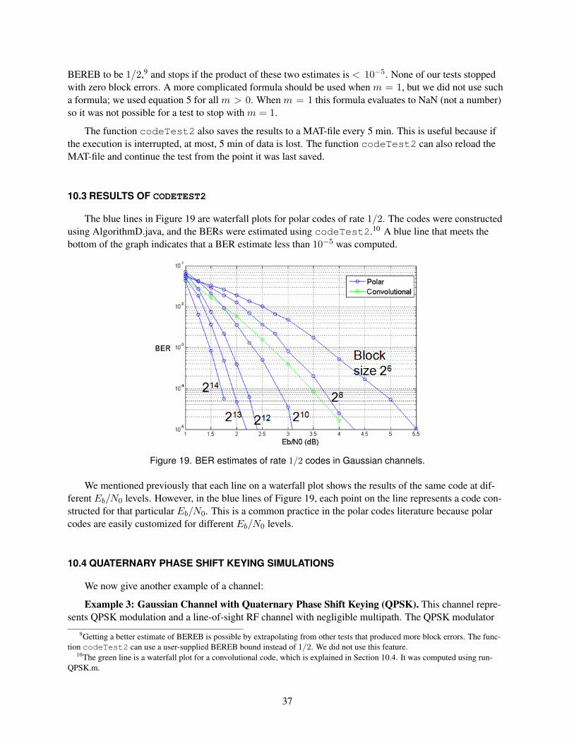
BEREB to be 1/2,9 and stops if the product of these two estimates is < 10−5. None of our tests stoppedwith zero block errors. A more complicated formula should be used when m = 1, but we did not use sucha formula; we used equation 5 for all m > 0. When m = 1 this formula evaluates to NaN (not a number)so it was not possible for a test to stop with m = 1.
The function codeTest2 also saves the results to a MAT-file every 5 min. This is useful because ifthe execution is interrupted, at most, 5 min of data is lost. The function codeTest2 can also reload theMAT-file and continue the test from the point it was last saved.
10.3 RESULTS OF CODETEST2
The blue lines in Figure 19 are waterfall plots for polar codes of rate 1/2. The codes were constructedusing AlgorithmD.java, and the BERs were estimated using codeTest2.10 A blue line that meets thebottom of the graph indicates that a BER estimate less than 10−5 was computed.
Figure 19. BER estimates of rate 1/2 codes in Gaussian channels.
We mentioned previously that each line on a waterfall plot shows the results of the same code at dif-ferent Eb/N0 levels. However, in the blue lines of Figure 19, each point on the line represents a code con-structed for that particular Eb/N0. This is a common practice in the polar codes literature because polarcodes are easily customized for different Eb/N0 levels.
10.4 QUATERNARY PHASE SHIFT KEYING SIMULATIONS
We now give another example of a channel:
Example 3: Gaussian Channel with Quaternary Phase Shift Keying (QPSK). This channel repre-sents QPSK modulation and a line-of-sight RF channel with negligible multipath. The QPSK modulator
9Getting a better estimate of BEREB is possible by extrapolating from other tests that produced more block errors. The func-tion codeTest2 can use a user-supplied BEREB bound instead of 1/2. We did not use this feature.
10The green line is a waterfall plot for a convolutional code, which is explained in Section 10.4. It was computed using run-QPSK.m.
37
first maps a pair of bits to a point in the in-phase/quadrature (I/Q) plane. There are several QPSK map-pings. We use (0, 0) 7→ (− 1√
2,− 1√
2), (0, 1) 7→ (− 1√
2, 1√
2), (1, 0) 7→ ( 1√
2,− 1√
2), (1, 1) 7→ ( 1√
2, 1√
2). The
I/Q point is then converted to a sinusoidal waveform that is transmitted. The receiver rescales the wave-form to compensate for the attenuation. The demodulator maps the waveform back to I/Q space, resultingin (± 1√
2+ nI ,± 1√
2+ nQ), where nI and nQ are random noise variables that are assumed to be indepen-
dent, normally distributed, with 0 mean and equal variance.
For any σ > 0, the Gaussian QPSK channel with noise variance σ2 has input set X = {0, 1}2, outputset Y = R2, and transition probabilities
W (y1, y2|u1, u2) =1
σ22πexp
−(y1 + (−1)u1√
2
)2+(y2 + (−1)u2√
2
)2
2σ2
.
Note that this is not a binary channel because it has more than two inputs. It is memoryless, and sym-metric in an appropriate sense.
Like the BPSK Gaussian channel, the QPSK Gaussian channel has the same Es/N0 = 12σ2 . However,
twice as much information is sent in each use of the channel, so Eb/N0 = N4σ2K
.
Section 4.8.4 of [27] shows that each use of the QPSK Gaussian channel is equivalent to two consecu-tive uses of the BPSK Gaussian channel with the same Eb/N0. So codeTest2 can simulate QPSK if weinterpret two consecutive bits as the I and Q components of the same signal. We also wrote runQPSK.m,a MATLAB R© script that explicitly simulates QPSK. This script can simulate polar coding, and it canalso simulate convolutional coding, using functions from the MATLAB R© Communications Toolbox. An(N,K, l) convolutional code is an FEC code that takes K bits as input and outputs N bits. However, theseN bits are determined not only by the input but also by the previous l − 1 inputs. Convolutional codes arenot block codes.
Figure 20 shows BER estimates computed with runQPSK.m. These include polar codes of three dif-ferent lengths. They also include two convolutional codes, a (2, 1, 7) and a (2, 1, 9). The former is used inseveral U.S. military communications systems (for example, see [26]).
10.5 SIMULINK R© RESULTS
We built Simulink R© models representing QPSK Gaussian channels. Figure 21 shows results for threedifferent FEC codes: a (1024, 512) turbo code, a (64800, 32400) LDPC code, and a (61, 51) Reed–Solomoncode.
38
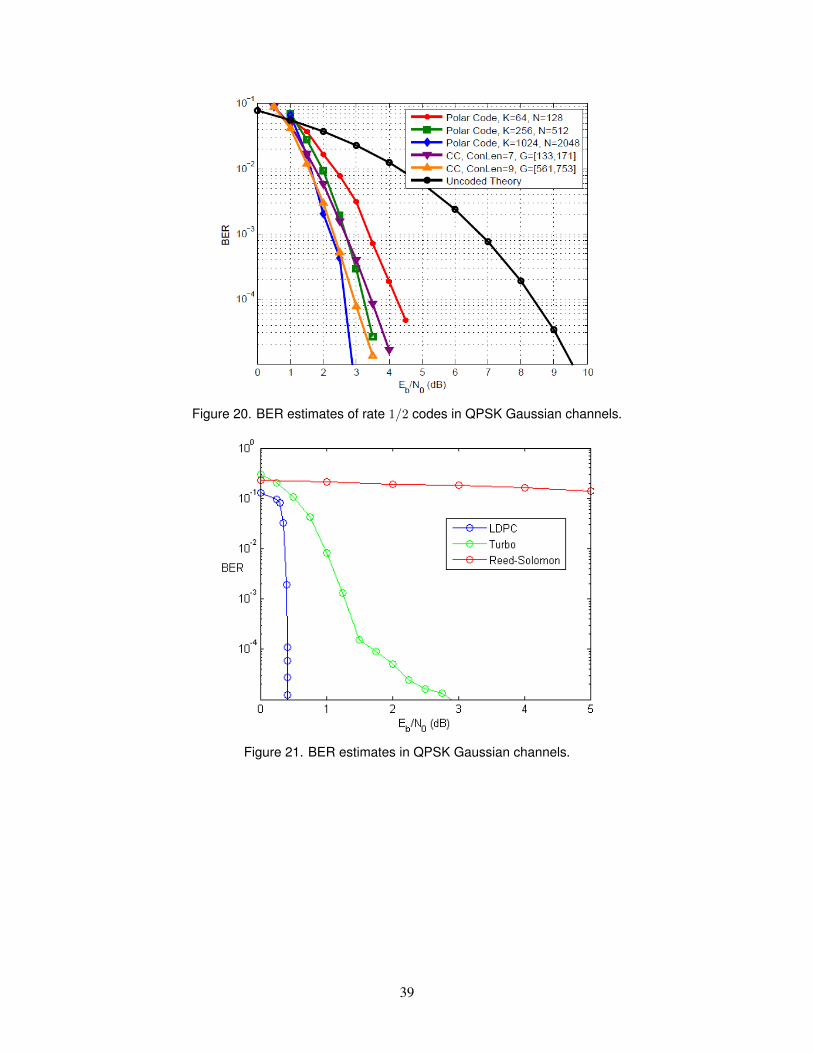
Figure 20. BER estimates of rate 1/2 codes in QPSK Gaussian channels.
Figure 21. BER estimates in QPSK Gaussian channels.
39


11. CONCLUSION
Our FY14 progress has consisted mostly of implementing published algorithms and reproducing pub-lished results. We have implemented and tested several methods for encoding, decoding, and code con-struction.
Our preliminary conclusion is that polar codes can outperform the FEC currently used in some modesof Navy communications systems. Polar codes may also be able to outperform other codes that could beused to replace the current codes. Polar codes are more likely to be useful at higher data rates. Further re-search is needed to test polar codes, using more realistic models of Navy systems and their RF environ-ments. We are now well positioned to do this further research.
41

43
REFERENCES
1. E. Arikan. 2009. “Channel Polarization: A Method for Constructing Capacity-Achieving Codes for Symmetric Binary-Input Memoryless Channels,” IEEE Transactions on Information Theory 55 (7):3051–3073. 2. D. Wasserman and A. Ahmed. 2014. “Polar Codes Source Codes.” Technical Document 3287. Space and Naval Warfare Systems Center Pacific (SSC Pacific), San Diego, CA. 3. R. W. Hamming. 1950. “Error Detecting and Error Correcting Codes,” Bell System Technical Journal 29(2):147–160. 4. C. Shannon. 1948. “A Mathematical Theory of Communication,” Bell Systems Technical Journal 27:379–423, 623–657. 5. I. Tal and A. Vardy. 2011. “List Decoding of Polar Codes.” Proceedings of the 2011 IEEE International Symposium on Information Theory (ISIT) (pp. 1–5), July 31–August 5, St. Petersburg, Russia. IEEE. 6. P. Trifonov. 2012. “Efficient Design and Decoding of Polar Codes,” IEEE Transactions on Communications 60(11):3221–3227. 7. A. Eslami and H. Pishro-Nik. 2011. “A Practical Approach to Polar Codes.” Proceedings of the 2011 IEEE International Symposium on Information Theory (ISIT) (pp. 16–20). July 31‒August 5, St. Petersburg, Russia. IEEE. 8. K. Niu. and K. Chen. 2012. “CRC-Aided Decoding of Polar Codes,” IEEE Communica-tions Letters 16(10):1668–1671. 9. K. Niu, K. Chen, and J.-R. Lin. 2013 “Beyond Turbo Codes: Rate-Compatible Punctured Polar Codes.” Proceedings of 2013 IEEE International Conference on Communications (ICC) (pp. 3423–3427). June 9–13, Budapest, Hungary. IEEE. 10. C. Leroux, I. Tal, A. Vardy, and W. Gross. 2011. “Hardware Architectures for Successive Cancellation Decoding of Polar Codes,” Proceedings of the 2011 IEEE International Conference on Acoustics, Speech and Signal Processing (ICASSP) (pp. 1665–1668). May 22–27, Prague, Czech Republic. IEEE. 11. A. Alamdar-Yazdi and F. R. Kschischang. 2011. “A Simplified Successive-Cancellation Decoder for Polar Codes,” IEEE Communications Letters 15(12):1378–1380. 12. C. Leroux, A. J. Raymond, G. Sarkis, I. Tal, A. Vardy, and W. J. Gross. 2012. “Hardware Implementation of Successive-Cancellation Decoders for Polar Codes,” Journal of Signal Processing Systems 69 (3):305–315. 13. B. Yuan and K. Parhi. 2014. “Low-Latency Successive-Cancellation Polar Decoder Architectures Using 2-Bit Decoding,” IEEE Transactions on Circuits and Systems I: Regular Papers 61(4):1241–1254.

17. Mishra, A., Raymond, A., Amaru, L., Sarkis, G., Leroux, C., Meinerzhagen, P., Burg, A., and Gross,W. 2012. “A Successive Cancellation Decoder ASIC for a 1024-Bit Polar Code in 180nm CMOS,”2012 IEEE Asian Solid State Circuits Conference (A-SSCC) (pp. 205–208).
18. Bravo-Santos, A. 2013. “Polar Codes for Gaussian Degraded Relay Channels,” IEEE CommunicationsLetters, vol. 17, no. 2, pp. 365–368.
19. Tal, I. and Vardy, A. 2013. “How to Construct Polar Codes,” IEEE Transactions on Information The-ory, vol. 59, no. 10, pp. 6562–6582.
20. Cormen, T. H., Leiserson, C. E., Rivest, R. L., and Stein, C. 2001. Introduction to Algorithms, vol. 2,MIT Press Cambridge.
21. Li, H. and Yuan, J. 2013. “A Practical Construction Method for Polar Codes in AWGN Channels,”2013 IEEE TENCON Spring Conference (pp. 223–226).
22. Wu, D., Li, Y., and Sun, Y. 2014. “Construction and Block Error Rate Analysis of Polar Codes OverAWGN Channel Based on Gaussian Approximation,” IEEE Communications Letters, vol. 18, no. 7,pp. 1099–1102.
23. Arikan, E. 2011. “Systematic Polar Coding,” IEEE Communications Letters, vol. 15, no. 8, pp. 860–862.
24. Sarkis, G. and Gross, W. 2013. “Increasing the Throughput of Polar Decoders,” IEEE Communica-tions Letters, vol. 17, no. 4, pp. 725–728.
25. Guimaraes, D. A. 2010. Digital Transmission: A Simulation-Aided Introduction with VisSim/Comm,Springer.
26. Department of Defense (DoD). 2011. Department of Defense Interface Standard MIL-STD-188-110C:Interoperability and Performance Standards for Data Modems, 23 September 2011.
27. Sklar, B. 2001. Digital Communications, vol. 2, Prentice Hall NJ.
44

5f. WORK UNIT NUMBER
REPORT DOCUMENTATION PAGEForm Approved
OMB No. 0704-01-0188
The public reporting burden for this collection of information is estimated to average 1 hour per response, including the time for reviewing instructions, searching existing data sources, gathering and maintaining the data needed, and completing and reviewing the collection of information. Send comments regarding this burden estimate or any other aspect of this collection of information, including suggestions for reducing the burden to Department of Defense, Washington Headquarters Services Directorate for Information Operations and Reports (0704-0188), 1215 Jefferson Davis Highway, Suite 1204, Arlington VA 22202-4302. Respondents should be aware that notwithstanding any other provision of law, no person shall be subject to any penalty for failing to comply with a collection of information if it does not display a currently valid OMB control number. PLEASE DO NOT RETURN YOUR FORM TO THE ABOVE ADDRESS.
1. REPORT DATE (DD-MM-YYYY) 2. REPORT TYPE 3. DATES COVERED (From - To)
4. TITLE AND SUBTITLE 5a. CONTRACT NUMBER
5b. GRANT NUMBER
5c. PROGRAM ELEMENT NUMBER
5d. PROJECT NUMBER
5e. TASK NUMBER
6. AUTHORS
7. PERFORMING ORGANIZATION NAME(S) AND ADDRESS(ES) 8. PERFORMING ORGANIZATION REPORT NUMBER
10. SPONSOR/MONITOR’S ACRONYM(S)
11. SPONSOR/MONITOR’S REPORT NUMBER(S)
9. SPONSORING/MONITORING AGENCY NAME(S) AND ADDRESS(ES)
12. DISTRIBUTION/AVAILABILITY STATEMENT
13. SUPPLEMENTARY NOTES
14. ABSTRACT
15. SUBJECT TERMS
16. SECURITY CLASSIFICATION OF: a. REPORT b. ABSTRACT c. THIS PAGE
17. LIMITATION OF ABSTRACT
18. NUMBER OF PAGES
19a. NAME OF RESPONSIBLE PERSON
19B. TELEPHONE NUMBER (Include area code)
Standard Form 298 (Rev. 8/98)Prescribed by ANSI Std. Z39.18
Dec
December 2014 Final
Polar Codes
David Wasserman
SSC Pacific, 53560 Hull Street, San Diego, CA 92152–5001
TR 2054
Naval Innovative Science and Engineering (NISE) Program (Applied Research) SSC Pacific, 53560 Hull Street, San Diego, CA 92152–5001
Approved for public release.
This is work of the United States Government and therefore is not copyrighted. This work may be copied and disseminated without restriction.
. The purpose of the project is to determine if polar codes can outperform the forward error correction (FEC) currently used in Navy wireless communication systems. This report explains polar codes to non-specialists. The project team has written and tested software that implements several published polar coding algorithms. For comparison, the team has also implemented and tested other forward error correction methods: a turbo code, a low density parity check (LDPC) code, a Reed–Solomon code, and three convolutional codes. The team’s preliminary conclusion is that polar codes can outperform the FEC currently used in some modes of Navy communications systems. Polar codes may also be able to outperform other codes that could be used to replace the current codes. Polar codes are more likely to be useful at higher data rates. Further research is needed to test polar codes, using more realistic models of Navy systems and their RF environments. Space and Naval Warfare Systems Center Pacific is now well positioned to do this further research.
Mission Area: Communications polar codes polar encoder polar construction Gaussian approximation method polar coding algorithms block codes polar decoder Tal/Vardy Method forward error correction
David Wasserman
U U U U 53 (619) 553-3003
INITIAL DISTRIBUTION
84300 Library (2) 85300 Archive/Stock (1) 56270 D. Wasserman (1)
Defense Technical Information Center Fort Belvoir, VA 22060–6218 (1)

Approved for public release.
SSC Pacific San Diego, CA 92152-5001


