Polarimetric Image Reconstruction Algorithms by John R. Valenzuela A dissertation submitted in partial fulfillment of the requirements for the degree of Doctor of Philosophy (Applied Physics) in The University of Michigan 2010 Doctoral Committee: Professor Jeffrey A. Fessler, Chair Professor Stephen C. Rand Associate Professor Selim Esedoglu Senior Scientist Brian J. Thelen, Michigan Tech Research Institute Chief Scientist Richard G. Paxman, General Dynamics – AIS
Transcript
Polarimetric Image Reconstruction Algorithms
by
John R. Valenzuela
A dissertation submitted in partial fulfillmentof the requirements for the degree of
Doctor of Philosophy(Applied Physics)
in The University of Michigan2010
Doctoral Committee:
Professor Jeffrey A. Fessler, ChairProfessor Stephen C. RandAssociate Professor Selim EsedogluSenior Scientist Brian J. Thelen, Michigan Tech Research InstituteChief Scientist Richard G. Paxman, General Dynamics – AIS
2.1 Noisy and blurred polarimetric imagery. The First row has an SNRof 25dB and the second row has an SNR of 15dB. From left to rightthe angle of the polarizer is 0, 45, 90, 135 . . . . . . . . . . . . 23
2.2 Estimates of Stokes images for SNR = 25dB. All rows read from leftto right: Pristine, Proposed Method, Traditional Method. First row:S0, second row: S1, third row: S2. . . . . . . . . . . . . . . . . . . . 24
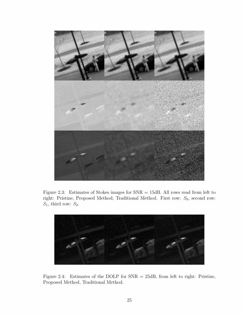
2.3 Estimates of Stokes images for SNR = 15dB. All rows read from leftto right: Pristine, Proposed Method, Traditional Method. First row:S0, second row: S1, third row: S2. . . . . . . . . . . . . . . . . . . . 25
2.4 Estimates of the DOLP for SNR = 25dB, from left to right: Pristine,Proposed Method, Traditional Method. . . . . . . . . . . . . . . . . 25
2.5 Estimates of the DOLP for SNR = 15dB, from left to right: Pristine,Proposed Method, Traditional Method. . . . . . . . . . . . . . . . . 26
2.6 Estimates of the DOLP for SNR = 25dB, from left to right: Pris-tine, Proposed method with cross channel regularization, Traditionalmethod with cross channel regularization. . . . . . . . . . . . . . . . 26
2.7 Estimates of the DOLP for SNR = 15dB, from left to right: Pris-tine, Proposed method with cross channel regularization, Traditionalmethod with cross channel regularization. . . . . . . . . . . . . . . . 26
3.1 Traditional phase-diversity imaging strategy. . . . . . . . . . . . . . 283.2 Geometry for defining the aberration function W (x, y). . . . . . . . 323.3 Polarimetric phase diversity strategy utilizing the division-of-focal-
3.9 Image estimation results for SNR = 45dB. From left to right: object,estimate using edge-preserving regularizer, estimate using quadraticregularizer, and the conventional estimate. . . . . . . . . . . . . . . 45
3.10 Image estimation results for SNR = 25dB. From left to right: object,estimate using edge-preserving regularizer, estimate using quadraticregularizer, and the conventional estimate. . . . . . . . . . . . . . . 45
3.11 Cuts through a column of TPOL for the object and reconstructionswith edge-preserving and quadratic regularization at SNR = 45dB. . 46
3.12 Cuts through a column of TPOL for the object and reconstructionswith edge-preserving and quadratic regularization at SNR = 25dB. . 47
3.13 Residual wavefront errors for SNR = 45dB. From left to right: edge-preserving regularization, quadratic regularization tuned for objectestimation, and quadratic regularization tuned for aberration esti-mation. . . . . . . . . . . . . . . . . . . . . . . . . . . . . . . . . . . 47
3.14 Residual wavefront errors for SNR = 25dB. From left to right: edge-preserving regularization, quadratic regularization tuned for objectestimation, and quadratic regularization tuned for aberration esti-mation. . . . . . . . . . . . . . . . . . . . . . . . . . . . . . . . . . . 47
4.1 Traditional phase-diversity imaging strategy. . . . . . . . . . . . . . 504.2 partitions of ∇[2,0]Φ and ∇[1,1]Φ . . . . . . . . . . . . . . . . . . . . 584.3 From left to right: pristine tank with subregion for processing indi-
cated by the red box, tank with 0.2 RMS waves of optical blur, tankwith 0.2 RMS waves of optical blur and additive noise to 25dB . . 63
4.4 From left to right: point object, point with 0.2 RMS waves of opticalblur, point with 0.2 RMS waves of optical blur and additive noise to5dB . . . . . . . . . . . . . . . . . . . . . . . . . . . . . . . . . . . 63
4.5 A particular wavefront realization in the Monte Carlo ensemble. . . 644.6 Individual aberration estimates and averaged estimates. . . . . . . . 654.7 Estimated standard deviation as a function of β. . . . . . . . . . . . 654.8 Comparison of the average of the estimate standard deviations calcu-
lated via both (4.43) and (4.30), as well as the RMSE of the MonteCarlo simulation, for the extended scene. . . . . . . . . . . . . . . . 67
4.9 Comparison of the average of the estimate standard deviations calcu-lated via both (4.43) and (4.30), as well as the RMSE of the MonteCarlo simulation, for the point object. . . . . . . . . . . . . . . . . . 68
B.1 Density plot of log(Ψ). . . . . . . . . . . . . . . . . . . . . . . . . . 83B.2 Density plot of log(Ψ) thresholded for enhanced color representation. 84
Fig. 2.1 show the noisy and blurred data for both SNR levels, Figs. 2.2 and 2.3
show estimates of the Stokes images for SNR levels of 25dB and 15dB respectively,
and Figs. 2.4 and 2.5 show estimates of the DOLP for SNR levels of 25dB and 15dB
respectively. Figs. 2.6 and 2.7 show estimates of the DOLP with the addition of cross-
channel regularization for both the proposed and traditional estimators for SNR levels
of 25dB and 15dB respectively.
22
Figure 2.1: Noisy and blurred polarimetric imagery. The First row has an SNR of25dB and the second row has an SNR of 15dB. From left to right the angle of thepolarizer is 0, 45, 90, 135
2.7 Conclusions and Future Work
Estimation of Stokes vectors directly provides estimates with lower overall RMS er-
ror as compared with restoring the intensity images and then transforming to Stokes
space for interpretation. The addition of a cross-channel regularization term im-
proves interpretability for both the proposed estimator and the tradtitional estimator
markedly. In the low (15dB) SNR regime the proposed estimator outperforms the
traditional estimator both with and without cross-channel regularization. Future
work includes addressing non idealities such aliasing and broadband optical PSF ef-
fects. Also, investigating estimator efficiency, convergence properties, and automatic
selection of regularization parameters will be done.
23
Figure 2.2: Estimates of Stokes images for SNR = 25dB. All rows read from left toright: Pristine, Proposed Method, Traditional Method. First row: S0, second row:S1, third row: S2.
24
Figure 2.3: Estimates of Stokes images for SNR = 15dB. All rows read from left toright: Pristine, Proposed Method, Traditional Method. First row: S0, second row:S1, third row: S2.
Figure 2.4: Estimates of the DOLP for SNR = 25dB, from left to right: Pristine,Proposed Method, Traditional Method.
25
Figure 2.5: Estimates of the DOLP for SNR = 15dB, from left to right: Pristine,Proposed Method, Traditional Method.
Figure 2.6: Estimates of the DOLP for SNR = 25dB, from left to right: Pristine,Proposed method with cross channel regularization, Traditional method with crosschannel regularization.
Figure 2.7: Estimates of the DOLP for SNR = 15dB, from left to right: Pristine,Proposed method with cross channel regularization, Traditional method with crosschannel regularization.
26
CHAPTER III
Phase-Diverse Polarimetric Image Reconstruction
3.1 Introduction
Polarimetric imaging systems acquire data that can be used to infer the polarization
state of an optical field [93, 7]. The polarization state of an optical field across a scene
contains information related to surface features such as shape and roughness [26].
Naturally occurring objects typically have a larger surface granularity than man-
made objects, so polarimetry offers the potential for improved target detection and
identification over other imaging modalities [37].
The polarization state of a transverse optical field can be specified by the Stokes
vector S = (S0, S1, S2, S3) [15, 45]. The elements of S are functions of the optical
intensity and defined in the following way: S0 is the total optical intensity, S1 is
the difference between the optical intensity transmitted by a linear polarizer with
pass axis oriented at 0 (reference) and one having pass axis oriented at 90, S2 is
the difference between the optical intensity transmitted by a linear polarizer with
pass axis oriented at 45 and one having pass axis oriented at 135, and S3 is the
optical intensity transmitted by a right circular polarizer and a left circular polarizer.
In the majority of remote-sensing applications the linear polarization state of the
optical field is of interest and so the S3 component is ignored. We adopt this usual
simplification of considering only the first three components of the Stokes vector,
27
though the method generalizes easily.
Polarimeters, like traditional incoherent imaging sensors, have resolution limits
that depend on noise and system point-spread function. In remote-sensing applica-
tions, degradations in the point-spread function are often due to atmospheric turbu-
lence, residual aberrations in the optical system or misalignment among components
in the optical system. We previously developed a method for estimating Stokes im-
ages directly from polarimetric measurements [97]. That work assumed complete
knowledge of the system point-spread function and was thus limited in its range of
application. In this paper, we propose methods that overcome this limitation by
introducing phase diversity into the polarimetric measurements. In traditional inco-
herent imaging the technique of phase diversity has been used to jointly estimate the
object and optical aberrations in the presence of atmospheric turbulence [69]. Phase
diversity requires the simultaneous collection of two or more images that are related
via a deterministic phase perturbation. Typically, two images are collected: one is
the conventional in-focus image and the second image is acquired on a separate focal
plane that is translated along the optical axis thereby inducing a known defocus to
the second image. Fig. 3.1 shows a typical phase diversity configuration. A direct ex-
Figure 3.1: Traditional phase-diversity imaging strategy.
tension of the traditional phase diversity strategy to polarimetry would be to acquire
28
two measurements per polarimetric channel; a four-channel polarimeter would be ex-
tended to an eight-channel polarimeter. Here we present two algorithms to jointly
estimate the Stokes vectors and optical aberrations using a simpler four-channel phase
diverse polarimeter. The method could be adapted easily to eight-channel polarime-
ters and other variations, but a four-channel polarimeter configuration is particularly
attractive in terms of cost and complexity of hardware.
One acquisition parameter that must be chosen is the amount of defocus in the
diversity channel(s). Choosing the optimal amount of phase diversity for phase-
diverse phase-retrieval in a traditional incoherent imaging system was investigated
in [53] using the Cramer-Rao lower bound. In this work we also use the Cramer-Rao
lower bound for phase-diverse phase-retrieval as a guide in choosing the amount of
defocus to introduce into the system.
For simplicity of presentation, all optical-system elements are assumed to be ideal
and all polarimetric measurements are assumed to be perfectly registered.
The organization of this paper is as follows. Section II presents the mathemati-
cal framework of joint estimation of object and aberrations from polarimetric mea-
surements. Section III formulates a reduced-parameter search strategy. Section IV
explores joint estimation numerically with both quadratic and edge-preserving regu-
larization. Sections V and VI give results and concluding remarks.
3.2 Mathematical Framework
3.2.1 Stokes-Vector Imaging
The optical intensity, Γ, at a single point in an imaging system with a linear
polarizer in the optical path having pass axis oriented at angle θ to the reference axis
29
can be expressed in terms of the Stokes vector,
Γ (θ) =1
2[S0 + S1 cos(2θ) + S2 sin(2θ)] . (3.1)
An imaging polarimeter has multiple channels, each with a different polarization
angle. For J measurements (channels) at polarization angles θ1, . . . , θJ , equation (3.1)
becomes a system of J equations. In matrix form the system is
Γ(θ1)
...
Γ(θJ)
=1
2
1 cos(2θ1) sin(2θ1)
......
...
1 cos(2θJ) sin(2θJ)
S0
S1
S2
. (3.2)
When Γ(θj), S0, S1, and S2 are images each of size N ×M , (3.2) can be configured
lexicographically to become
Γ =(TJ×3 ⊗ Inp
)S, np = NM, (3.3)
where S = (S0, S1, S2) is a 3np × 1 column vector, Inp is the np × np identity matrix,
⊗ is the Kronecker product, TJ×3 is the matrix in (3.2), and Γ is a Jnp × 1 column
vector. The conventional estimate of the Stokes images, Sconv, is formed by using the
pseudo-inverse of TJ×3 [15]
Sconv =
[(T′J×3TJ×3)−1T′J×3
]⊗ Inp
Γ, (3.4)
where “ ′ ” denotes conjugate transpose. The matrix inverse in (3.4) is guaranteed to
exist if J ≥ 3 and the θj are chosen so that TJ×3 has linearly independent columns.
In words, in (3.4) the J × 3 system of equations in (3.2) is solved by least-squares at
each voxel independently.
30
3.2.2 Forward-Imaging Model
The model (3.3) ignores measurement blur and noise. A more complete discrete-
discrete forward model for an incoherent imaging system that accounts for space-
invariant optical blur and additive noise can be represented by 2D discrete convolu-
tion:
yj(n,m) = bj(n,m) ∗ Γj(n,m) + εj(n,m) n = 1, . . . , N, m = 1, . . . ,M (3.5)
where yj(n,m) is the data for the jth channel, bj(n,m) denotes the incoherent point-
spread function associated with the jth channel, Γj(n,m) is the jth channel ideal
intensity image, ∗ denotes 2D convolution, and εj(n,m) is additive noise. A matrix-
vector representation of (3.5) is
yj = Bj
[(TJ×3)j ⊗ Inp
]S + εj, j = 1, . . . , J, (3.6)
where Bj denotes a np×np Toeplitz matrix whose entries depend on bj(n,m), (TJ×3)j
denotes the jth row of TJ×3, and εj is an additive noise vector. Stacking J channels
(each given by (3.6)) yields
y = B(TJ×3 ⊗ Inp
)S + ε (3.7)
where y4=(y1, . . . ,yJ), B
4= diagBj is a block diagonal matrix with the single-
channel blur matrices on the diagonal, and ε4=(ε1, . . . , εJ).
3.2.3 Point-Spread-Function Parameterization
Ideally the matrices Bj (or equivalently the PSFs bj(n,m)) would correspond to
diffraction-limited PSFs. In practice the PSF is often degraded by known or unknown
aberrations. In the presence of aberrations the generalized pupil function for the
31
system can be written
P(x, y) = A(x, y) exp [ıW (x, y)] , (3.8)
where A(x, y) is a binary aperture function and W (x, y) is an effective optical path-
length error. Figure 3.2 shows the geometry that defines the aberration function W .
If the system had no aberrations the exit pupil would have a perfect spherical wave
emanating from it towards the focal plane. However, when aberrations are present
the wavefront leaving the exit pupil departs from the spherical ideal. The aberration
function W (x, y) is the path-length error, with respect to a Gaussian reference sphere,
accumulated as a ray passes from the reference sphere to the actual wavefront [43]. It
Gaussian referencesphere
Ideal image point
Exitpupil
Actualwavefront
W(x,y)
Figure 3.2: Geometry for defining the aberration function W (x, y).
is a well known property of space-invariant optical imaging systems that the coherent
transfer function is a scaled version of the generalized pupil function and can be
32
written
H(u, v) = A(u, v) exp [ıW (u, v)] , (3.9)
where (u, v) are frequency domain coordinates [43]. Aberrations in an optical system
can be represented using a suitable basis set ϕk(u, v), such as Zernike polynomi-
als [60]. Representing W (u, v) in the basis ϕk(u, v) parameterizes the generalized
pupil function:
H(u, v;α) = A(u, v) exp
[ı
K∑k=1
αkϕk(u, v)
]where α = (α1, . . . , αK). (3.10)
Visible regime polarimeter configurations, such as division-of-focal-plane and division-
of-amplitude, simultaneously acquire all of the polarimetric channels and so are ex-
posed to identical optical aberrations, i.e., W (u, v) is the same for each channel.
3.2.4 Phase Diversity
To aid in the estimation of aberrations, we propose to introduce phase diversity,
typically by different amounts in the different polarimetric channels. Figs. 3.3 and 3.4
show two possible polarimetric-phase-diverse imaging strategies. If the phase diver-
sity function in channel j is denoted φj(u, v), then the generalized pupil function for
the jth channel can be written
Hj(u, v;α) = A(u, v) exp
ı
[K∑k=1
αkϕk(u, v) + φj(u, v)
]. (3.11)
The corresponding incoherent point-spread function, hj(x, y), and the optical
transfer function, Hj(u, v), can be written in terms of the generalized pupil func-
33
Figure 3.3: Polarimetric phase diversity strategy utilizing the division-of-focal-planetechnique.
tion:
hj(x, y;α) = c∣∣F−1 [Hj(u, v;α, φj)]
∣∣2 (3.12)
Hj(u, v;α) = c F[∣∣F−1 [Hj(u, v;α, φj)]
∣∣2] (3.13)
where F[·] is the Fourier transform and c is a constant that normalizes the point-
spread function to unit volume [53]. The modeled system point-spread function,
bj(n,m), and optical transfer function consist of samples of hj(x, y;α) and Hj(u, v;α)
at the Nyquist sampling rate [43], respectively. Consequently, each blur matrix, Bj, is
parameterized by the vector α. For analysis and implementation we assume periodic
boundary conditions on the object so that the blur matrices, Bj(α), are circulant
34
Figure 3.4: Polarimetric phase diversity strategy utilizing the division-of-amplitudetechnique.
and thus diagonalized by a 2D DFT matrix
Bj(α) = Q Ωj(α) Q′, (3.14)
where Q is a 2D unitary DFT matrix and Ωj(α) is a diagonal matrix whose entries
are the DFT coefficients of the first column of Bj(α).
3.3 Algorithms for Joint Estimation of Stokes Images and
Aberrations
This section describes novel algorithms for estimating S and α jointly under the
model (3.7). Under an additive Gaussian noise model εj ∼ N(0, σ2Inp) for j =
1, . . . , J , the log-likelihood function for both the object S and aberration parameters
35
α is
L(S,α) = − 1
2σ2
∥∥y −B(α)(TJ×3 ⊗ Inp
)S∥∥2. (3.15)
Conventional maximum-likelihood estimation is ineffective for this problem because
B(α) is ill-conditioned. Therefore we focus on penalized-likelihood estimators of the
form (S, α
)= argmin
(S,α)
− L(S,α) +R(S)
4= argmin
(S,α)
Ψ (S,α) (3.16)
where R(S) is a regularization term that penalizes an object, S, according to how
much it departs from our assumptions about the image properties [28]. In remote
sensing α is often a nuisance parameter. However, in an adaptive-optics system with
aberration correction capability, α is a parameter of interest. Depending on the
task at hand, either α or S or both can be parameters of interest. The choice of
regularization penalty will in general depend on the task, i.e., which parameters are
of interest and which are nuisance.
3.3.1 α as a Nuisance Parameter
When the Stokes images, S, are primary interest, then α is a nuisance parameter
and a regularization function that reflects a priori knowledge about the object should
be chosen. Stokes images (S1, S2) typically have sharp edges due to man-made objects
having stronger polarimetric signatures than naturally occurring objects. To recover
as much polarization information as possible the regularization function, R(S), should
preserve edges. Since quadratic regularization tends to wash out edges and smooth
noise we explore edge-preserving regularization using a hyperbolic potential function
ψ(t; δ) = δ2
(√1 +
(tδ
)2 − 1
). For fixed δ this function is approximately quadratic
for values of t < δ and approximately linear for t > δ. This behavior will tend to
36
smooth noise and preserve edges. Specifically, we chose R(S) be
R(S) =2∑l=0
2np∑k=1
βl ψ ([CSl]k; δl) , (3.17)
where C is a 2D finite-differencing matrix (horizontal and vertical differences). The
estimator (3.16) is then
(S, α
)= argmin
(S,α)
1
2σ2
∥∥y −B(α)(TJ×3 ⊗ Inp
)S∥∥2 +
2∑l=0
2np∑k=1
βl ψ ([CSl]k; δl). (3.18)
3.3.2 α As a Parameter of Interest — Reduced Parameter Search Strat-
egy
In [42] it was shown that, for a two channel phase-diversity system under an addi-
tive Gaussian noise model, the estimate of the object being imaged could be expressed
in terms of the system aberration parameters. This result was generalized in [69] for
phase-diverse imaging with an arbitrary number of channels. A similar procedure can
be used to derive a closed-form expression for the Stokes images in terms of system
aberrations for polarimetric phase-diverse imaging. Deriving this closed-form expres-
sion requires the use of a quadratic regularizer that can be diagonalized by the DFT
as in (3.14). We focus on quadratic regularizers of the form
R(S) =1
2
∥∥(√β3 ⊗C)S
∥∥2, (3.19)
where√β3
4= diag
√β0,√β1,√β2 and βi > 0 i = 0, 1, 2. Using this regularization
function (3.16) becomes
(S, α
)= argmin
(S,α)
1
2σ2
∥∥y −B (α)(TJ×3 ⊗ Inp
)S∥∥2
+1
2
∥∥(√β3 ⊗C)S
∥∥2. (3.20)
37
For a fixed aberration vector, α, (3.20) is convex in S and the column gradient of S
satisfies the stationary point condition ∇SΨ(S;α) = 0, where Ψ is defined in (3.16),
which leads to
S(α) =[(
T′J×3 ⊗ Inp
)B (α)′B (α)
(TJ×3 ⊗ Inp
)+ σ2β3 ⊗C′C
]−1
×(T′J×3 ⊗ Inp
)B (α)′ y.
(3.21)
The matrix inverse in (3.21) is guaranteed to exist provided the intersection of the
null spaces of the component matrices is the zero vector. Because C is a first-order
finite differencing matrix, the only nonzero vectors in its null space are of the form
γ1 where γ ∈ R and 1 is the np × 1 vector of ones. Therefore, nonzero vectors in
the null space of (√β3 ⊗ C) are of the form v = (γ11, γ21, γ31) where γ1, γ2, γ3
are not all simultaneously zero. It remains to show that v is not in the null space of(T′J×3 ⊗ Inp
)B (α)′B (α)
(TJ×3 ⊗ Inp
). Now,
(T′J×3 ⊗ Inp
)B (α)′B (α)
(TJ×3 ⊗ Inp
)v
=(T′J×3 ⊗ Inp
)QΩ (α)′Ω (α) Q′
(TJ×3 ⊗ Inp
)v︸ ︷︷ ︸
u
,
where the circulant approximation has been used. Observe that u is nonzero only
in the DC components. Recall that the optical transfer function, Ωj (α), for space-
invariant blur conserves energy and thus does not alter DC components. Thus,
(T′J×3 ⊗ Inp
)QΩ (α)′Ω (α)u =
(T′J×3 ⊗ Inp
)v 6= 0
since v is a nonzero constant vector.
Substitution of (3.21) into (3.20) yields an “aberration only” objective function,
α = argminα
1
2σ2
∥∥y−B (α)(TJ×3 ⊗ Inp
)S(α)
∥∥2+
1
2
∥∥(√β3⊗C)S(α)
∥∥2. (3.22)
38
The estimate in (3.22) is a joint estimate of object and aberrations, that is, mini-
mization over α implicitly minimizes over S. Once α has been estimated the object
estimate is given by (3.21). We note that this algorithm is a special case of the
variable projection method [39].
3.4 Simulation Experiments
We performed simulation experiments to evaluate joint estimation with both edge-
preserving regularization (3.18) and quadratic regularization (3.22). The simulations
were conducted using the circulant approximation, this approximation was facilitated
by tapering the object to its mean at the boundaries. Two situations were considered:
1. the object parameters are of interest and the aberration parameters are nuisance
parameters, and 2. the aberration parameters are of interest and the object param-
eters are nuisance parameters. Because of the significant computational savings af-
forded by (3.22) we evaluated it with distinct regularization tuned for each object and
aberrations. For comparison we also evaluated the conventional estimate (3.4) using
the same data without phase diversity. For ground truth, we used polarimetric images
collected using a division-focal-plane polarimeter by General Dynamics Advanced In-
formation Systems, Ypsilanti, MI. The linear polarizer pass axes were oriented at
0, 45, 90, 135, and the subsampled polarimetric image size was [256× 256] (sub-
sampled from a [512 × 512] micropolarizer array). The imagery was then corrupted
by space-invariant optical blur and additive zero-mean Gaussian noise. The optical
blur was constructed using an annular pupil with a phase distortion constructed from
Zernike polynomials 4-19 as defined in [60]; the phase distortion had an RMS strength
of 0.2 waves. The phase of the generalized pupil function is shown in Fig. 3.5. We
define the SNR of an image to be 20 log10(‖y‖ / ‖y − y‖)dB where y and y are the
noise free and noisy images respectively; the experiments were done at two SNR levels:
39
[waves]
−0.2
0
0.2
0.4
0.6
0.8
1
Figure 3.5: Phase of the generalized pupil function in units of waves.
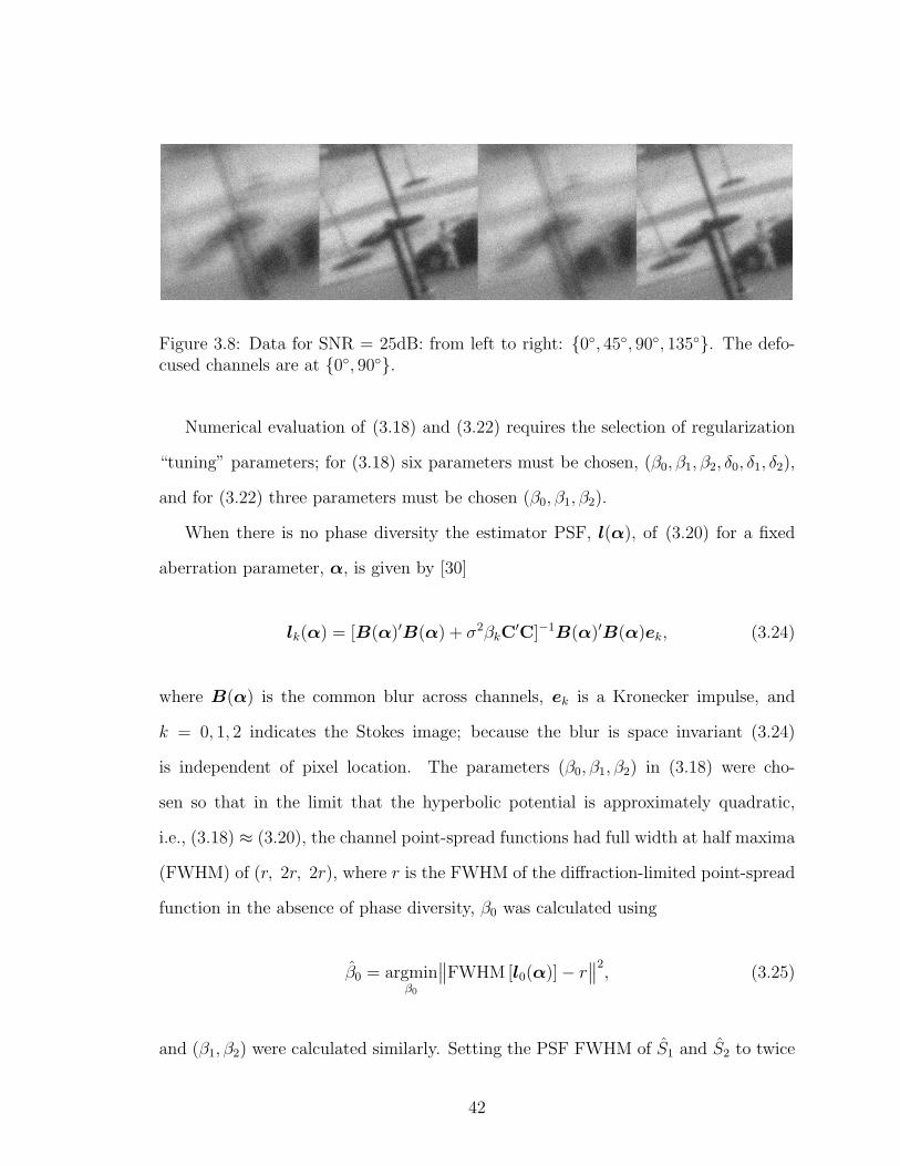
45dB and 25dB. To emulate a traditional phase-diversity configuration the defocused
channels were at angles 0, 90. In this configuration the 45, 135 channels sum
to form the conventional in-focus channel and the 0, 90 channels sum to form the
de-focus channel, see Fig. 3.7. To aid in selecting the amount of defocus to use in the
diversity channels we assumed complete knowledge of the object, as in the problem
of phase retrieval, in Figs. 3.9 and 3.10 (phase-diverse phase-retrieval) and computed
the Cramer-Rao bound for the aberration parameters over a range of defocus values
optimized for the estimation of α. The Fisher-information matrix is computed from
the log-likelihood function in (3.20)
F =1
σ2[∇αµ(α)] [∇αµ(α)]′ (3.23)
where ∇ denotes the column gradient and µ(α)4= B(α)
(T4×3 ⊗ Inp
)S. The Fisher-
information matrix was computed and inverted for various values of defocus. Since the
Zernike polynomials are orthonormal, the mean of the diagonal elements corresponds
40
to the minimum achievable mean-squared error, WMIN, of any unbiased estimator of
the degrading wavefront W (α). In Fig. 3.6 WMIN is plotted against peak-to-valley
defocus. The minimum occurs when the amount of defocus is 1.8 waves peak-to-
valley; we used this amount of defocus in the simulations but we note that it is
not necessarily the optimal choice for joint estimation of object and aberrations. The
blurry and noisy data with and without phase diversity are shown in Figs. 3.7 and 3.8.
0 0.5 1 1.5 2 2.5 3 3.5 4 4.5 50
0.1
0.2
0.3
0.4
0.5
0.6
0.7
Defocus [waves]
MS
E[w
aves]
Figure 3.6: Minimum mean squared error as a function of defocus measured frompeak to valley, both axes are in units of waves.
Figure 3.7: Data for SNR = 45dB: from left to right: 0, 45, 90, 135. The defo-cused channels are at 0, 90.
41
Figure 3.8: Data for SNR = 25dB: from left to right: 0, 45, 90, 135. The defo-cused channels are at 0, 90.
Numerical evaluation of (3.18) and (3.22) requires the selection of regularization
“tuning” parameters; for (3.18) six parameters must be chosen, (β0, β1, β2, δ0, δ1, δ2),
and for (3.22) three parameters must be chosen (β0, β1, β2).
When there is no phase diversity the estimator PSF, l(α), of (3.20) for a fixed
where B(α) is the common blur across channels, ek is a Kronecker impulse, and
k = 0, 1, 2 indicates the Stokes image; because the blur is space invariant (3.24)
is independent of pixel location. The parameters (β0, β1, β2) in (3.18) were cho-
sen so that in the limit that the hyperbolic potential is approximately quadratic,
i.e., (3.18) ≈ (3.20), the channel point-spread functions had full width at half maxima
(FWHM) of (r, 2r, 2r), where r is the FWHM of the diffraction-limited point-spread
function in the absence of phase diversity, β0 was calculated using
β0 = argminβ0
∥∥FWHM [l0(α)]− r∥∥2, (3.25)
and (β1, β2) were calculated similarly. Setting the PSF FWHM of S1 and S2 to twice
42
that of S0 is reasonable because of the significantly lower SNR in the S1 and S2 images.
We generated 20 realizations of α each having RMS phase strengths of 0.2 waves over
the pupil. For each aberration realization, (3.25) was solved numerically, then the
final values for (β0, β1, β2) were determined by averaging over the ensemble. Once the
β parameters were fixed the nonquadratic regularization parameters, δ0, δ1, δ2, were
determined by a brute-force multidimensional search for the parameter combination
which minimized the normalized RMS error between the Stokes object and the Stokes
estimate.
For (3.22) there were three regularization parameters to set for each case. These
parameters were determined by a brute-force multidimensional search for the param-
eter combination which minimized the normalized RMS error between 1. the Stokes
object and the Stokes estimate, and 2. the true aberrations and the aberration es-
timate. The regularization parameters that were “tuned” for object estimation were
10 orders of magnitude larger than those for aberration estimation.
After the regularization parameters were set, the estimators were evaluated over a
20 realization noise ensemble for each of two SNR levels. The initial estimate in each
case was formed using (3.4) with the phase-diverse data. Since closed form expres-
sions for the minimizers of (3.18) and (3.22) are not tractable they were minimized
numerically. The optimization was done using the limited memory Broyden-Fletcher-
Goldfarb-Shanno (L-BFGS) algorithm [57]. The minimization of (3.18) required pre-
conditioning due to the different scales of the Stokes images and the aberration pa-
rameters. Samples of the Hessian matrix of (3.18) were calculated via finite differences
and used in a diagonal preconditioner. The iterative search was stopped when the
iteration, k, satisfied (Ψk+1 −Ψk)/Ψk < 10−10, this corresponded to ≈ 200 iterations
for (3.18) and ≈ 30 iterations for (3.22).
43
3.5 Results
Tables 3.1 and 3.2 show normalized RMS estimation errors for each of (3.18),
(3.22), and (3.4). The reported errors are of the quantities S0, the total linear polar-
ization (TPOL)√S2
1 + S22 , and wavefront. There is no wavefront error to be reported
for the conventional estimate, (3.4), so a value of N/A is listed. Also, the estimates
of S0 and TPOL are listed as N/A for (3.22) when the regularization was tuned for
aberration estimation because the estimated images are unrecognizable. The poor
object estimates in this case are due to the small values of the regularization param-
eter. Recall that the object estimate is given by (3.21) which approaches the inverse
filter as β → 0 and thus greatly amplifies noise. The aberration estimation errors
for (3.22) when tuned for object estimation were reasonably good and are included
for completeness.
Table 3.1: RMS Error Percentages for SNR = 45dB
cost parameter of interest S0
√S2
1 + S22 wavefront
edge-preserving S 1.8%± 0.01% 36%± 0.3% 3.3%± 0.2%quadratic S 1.6%± 0.01% 40%± 0.2% 3.0%± 0.2%quadratic α N/A N/A 1.4%± 0.2%conventional estimate S 10%± 0.0013% 60%± 0.11% N/A
Table 3.2: RMS Error Percentages for SNR = 25dB
cost parameter of interest S0
√S2
1 + S22 wavefront
edge-preserving S 6.2%± 0.2% 59%± 1.4% 80%± 4.6%quadratic S 6.5%± 0.02% 61%± 1.0% 79%± 0.36%quadratic α N/A N/A 16%± 7%conventional estimate S 11%± 0.011% 490%± 1.7% N/A
Figs. 3.9 and 3.10 show object estimates for SNR = 45dB and SNR = 25dB
respectively. Each estimate is displayed in RGB format with the RGB channels set
44
as [S0+10√S2
1 + S22 , S0, S0]; in this display scheme the polarized elements of the scene
are red while the unpolarized elements are in gray scale; the factor of 10 in the red
channel was chosen for visual appeal. As expected, the estimates with data at a higher
SNR have lower RMS errors and are more visually appealing. Figs. 3.11 and 3.12
show cuts through TPOL reconstructions, at a column having an edge with large
polarization content, for SNR = 45dB and SNR = 25dB respectively. The benefit of
edge-preserving regularization is apparent in both cases but more pronounced at the
25dB SNR level as the quadratically regularized estimate shows significantly larger
blurring across the edge. Figs. 3.13 and 3.14 show the residual wavefronts, that is,
Figure 3.9: Image estimation results for SNR = 45dB. From left to right: object,estimate using edge-preserving regularizer, estimate using quadratic regularizer, andthe conventional estimate.
Figure 3.10: Image estimation results for SNR = 25dB. From left to right: object,estimate using edge-preserving regularizer, estimate using quadratic regularizer, andthe conventional estimate.
45
50 100 150 200
0.1
0.2
0.3
0.4
0.5
0.6
0.7
0.8
0.9
1
Row index
TP
OL [norm
aliz
ed to o
bje
ct]
object
edge−preserving
quadratic
Figure 3.11: Cuts through a column of TPOL for the object and reconstructions withedge-preserving and quadratic regularization at SNR = 45dB.
the estimated wavefront less the true wavefront. The estimates in all cases have lower
RMS errors with higher SNR data. At 45dB SNR the wavefront estimation errors
are all comparable. At 25dB SNR the wavefront error in using (3.22) (when tuned
for aberration estimation) is markedly lower than (3.18) and (3.22) (when tuned for
object estimation). This significant reduction in estimation error can be attributed
to the regularization being tuned for aberration estimation.
46
50 100 150 200
0.1
0.2
0.3
0.4
0.5
0.6
0.7
0.8
0.9
1
Row index
TP
OL [norm
aliz
ed to o
bje
ct]
object
edge−preserving
quadratic
Figure 3.12: Cuts through a column of TPOL for the object and reconstructions withedge-preserving and quadratic regularization at SNR = 25dB.
[wa
ve
s]
−0.03
−0.02
−0.01
0
0.01
Figure 3.13: Residual wavefront errors for SNR = 45dB. From left to right: edge-preserving regularization, quadratic regularization tuned for object estimation, andquadratic regularization tuned for aberration estimation.
[wa
ve
s]
−0.8
−0.6
−0.4
−0.2
0
0.2
Figure 3.14: Residual wavefront errors for SNR = 25dB. From left to right: edge-preserving regularization, quadratic regularization tuned for object estimation, andquadratic regularization tuned for aberration estimation.
47
3.6 Conclusions and Future Work
This paper has described two methods, (3.18) and (3.22), for joint estimation of
Stokes images and aberrations from polarimetric images with phase diversity. Estima-
tion accuracy follows a task-based hierarchy, i.e., in a joint-estimation framework the
choice of algorithm is task dependent. When the task is image restoration (aberrations
are nuisance parameters) an algorithm that jointly estimates object and aberrations
while incorporating a priori knowledge of the object is appropriate. However, if the
aberration parameters are of interest and the object is a nuisance parameter then
a reduced-parameter algorithm should be chosen. We mention that there contrived
situations for which aberration estimation in this context will fail. One such circum-
stance is when the scene is polarized in such a way that the diversity channel receives
little or no signal. For example, for a fixed set of polarizer angles 0, 45, 90, 135,
if the object is completely polarized along the reference axis (0), 90 channel will
have zero signal; if that channel is the diversity channel the ambiguity in the problem
will not be broken and the aberrations will not be able to be estimated.
Future work includes analyzing the bias and covariance of (3.20) and using those
expressions to investigate how the choice of diversity channels impacts estimation of
Stokes images and aberrations.
48
CHAPTER IV
Approximation to the object-aberration joint
covariance matrix in the phase-diversity context
4.1 Introduction
Incoherent imaging systems have resolution limits that depend, among other
things, on known or unknown phase aberrations. Phase aberrations arise from a
variety of sources including atmospheric turbulence, misaligned optics within the sys-
tem, improper mirror figure, and sub-aperture misalignments in multi-aperture sys-
tems [40]. Knowledge of system phase aberrations affords either correction through
the use of adaptive optics (AO), or post-detection deblurring of the collected imagery
via image restoration algorithms.
Phase diversity is an image-based wavefront-sensing technique that allows for the
joint estimation of object and phase aberrations. The technique of phase diversity
requires the simultaneous collection of two or more images that are related via a
deterministic phase perturbation. In the canonical phase diversity configuration, two
images are collected: one is the conventional in-focus image and the second image is
acquired on a separate focal plane that is translated along the optical axis thereby
inducing a known defocus to the second image, see figure 4.1.
For telescopes that require wavefront sensors, such as, telescopes that employ
49
extended object
beam splitter
known defocus
conventional image
diversity image
atmosphericdegradation
Figure 4.1: Traditional phase-diversity imaging strategy.
AO correction or multi-aperture telescopes that require sub-aperture phasing, phase
diversity is a candidate wavefront sensor [71]. When implementing a phase-diverse
wavefront sensor there are several acquisition parameters that must be chosen, such
as, the type and strength of phase diversity. Several analyses have been done to
address the optimality of acquisition parameters in the Cramer-Rao sense [53, 21,
20, 22, 19], however, these analyses assume complete knowledge of the object being
imaged and therefore may give misleading results. Moreover, many phase-diverse
wavefront sensors are biased estimators which are not bounded in variance by the
classical Cramer-Rao lower bound. An attractive class of phase-diverse wavefront
sensors are quadratically regularized weighted least squares estimators, this is due to
the availability of a reduced parameter formulation of the estimator that is explicitly
dependent on only the aberrations being estimated. In this paper we present an
approximation to the joint covariance matrix for a quadratically regularized weighted
least squares phase-diverse wavefront sensor; we use this approximation as an analysis
tool for aberration estimation performance in the presence of an unknown object.
The organization of this chapter is as follows: In section 2 we review the phase
diversity concept and algorithms. In section 3 we review approximations to the bias
and covariance of implicitly defined estimators. In section 4 we develop an expression
50
for the covariance of aberration estimates for a quadratically regularized weighted
least squares phase-diverse wavefront sensor. In section 5 we present simulation ex-
periments, and in sections 6 and 7 we present results and conclusions.
4.2 Review of the phase diversity concept
The technique of phase diversity was first proposed by Gonsalves [42, 41] and
was later generalized and put into the framework of maximum-likelihood estimation
by Paxman [69]. As an explicit maximum-likelihood estimator (MLE) of object and
aberrations phase diversity is not a viable wavefront sensing technique owing to the
large number of parameters that must be jointly estimated (object pixels + aberration
parameters). The viability of phase diversity as an ML wavefront sensor comes from
the availability of a closed-form expression for the object in terms of the aberration
parameters. In an ML framework that assumes additive Gaussian noise, the implicit
function theorems can be invoked and a closed-form expression for the object, in terms
of the aberration parameters, can be written . Back substitution of this expression
into the MLE reduces the dimensionality of the estimation problem down to only the
number of aberration parameters. For completeness we briefly restate these results
in the framework of linear algebra.
4.2.1 Forward imaging model
A discrete-discrete forward model for the jth channel of a J channel incoherent
imaging system that includes phase diversity, accounts for space-invariant optical
blur, and additive noise can be represented by
yj = tjBj(α)S + εj, j = 1, . . . , J, (4.1)
51
where yj is an (nd × 1) lexicographically ordered data vector, Bj(α) denotes an
(np × np) Toeplitz matrix that is parameterized by the vector α = (α1, . . . , αK), S is
an (np×1) lexicographically ordered object vector , εj is an (np×1) lexicographically
ordered noise vector, nd is the number of collected pixels, and np is the number of
object pixels. Stacking J channels (each given by (4.1)) yields
y = B(α)(TJ ⊗ Inp
)S + ε (4.2)
where y4=(y1, . . . ,yJ), TJ
4=(t1, . . . , tJ), B(α)
4= diagBj(α) is a block diagonal ma-
trix with the single-channel blur matrices on the diagonal, Inp is the np × np identity
matrix, ε4=(ε1, . . . , εJ), and ⊗ is the Kronecker product.
To aid in the analysis we make the common additional approximation that the
Bj(α) are circulant and are thus diagonalized by the unitary 2D-DFT matrix. We
discuss the parameterization of the Bj(α) in detail in the next section.
4.2.2 Phase aberration parameterization in the phase diversity context
Phase aberrations in a space-invariant incoherent imaging system are conveniently
represented through the generalized pupil function [43]. Let the continuous-space
generalized pupil function (also the coherent transfer function in this case) be denoted
by H(u, v), then
H(u, v) = P (u, v) exp [ıW (u, v)] , (4.3)
where P (u, v) is a binary aperture function, W (u, v) is a phase aberration function
proportional to an effective optical path-length error, and (u, v) are frequency domain
coordinates [43]. The phase aberration function, W , can be parameterized by repre-
senting it in an appropriate basis. Using a suitable basis, ϕk(u, v), W (u, v) can be
52
expanded leading to
H(u, v;α) = P (u, v) exp
[ıK∑k=1
αkϕk(u, v)
]where α = (α1, . . . , αK). (4.4)
If the phase diversity function in channel j is denoted φj(u, v), then the generalized
pupil function for the jth channel can be written
Hj(u, v;α) = P (u, v) exp
ı
[K∑k=1
αkϕk(u, v) + φj(u, v)
]. (4.5)
The continuous-space optical transfer function, Hj(u, v), is then
Hj(u, v;α) = c F[∣∣F−1 [Hj(u, v;α)]
∣∣2] , (4.6)
where F[·] is the Fourier transform and c is a constant that ensures that the corre-
sponding point-spread function is normalized to unit volume [53]. Let Ωj(α) denote
an (np×np) diagonal matrix consisting of samples of (4.6) taken at the Nyquist rate.
Then, by invoking the circulant approximation we may write
Bj(α) = Q Ωj(α) Q′ (4.7)
where Q is the unitary 2D-DFT matrix and ′ indicates conjugate transpose. Conse-
quently, each blur matrix, Bj, is parameterized by the vector α.
53
4.2.3 Maximum-likelihood framework
Under the noise model ε ∼ N(0,Kε) a maximum-likelihood estimate of the joint
parameter vector, [S,α], for the imaging model (4.2) is given by
[S, α] = argmin(S,α)
Φ(S,α) (4.8)
= argmin(S,α)
1
2
∥∥y −B(α)(TJ ⊗ Inp)S∥∥2
K−1ε, (4.9)
where Kε is assumed to be nonsingular. For a fixed aberration vector, α, (4.9) is
convex in S and so satisfies the stationary-point condition ∇SΦ(S, ·) = 0. Using this
condition an expression for the object in terms of the aberration parameters can be
derived:
S(α) =[T′JB
′(α)K−1ε B(α)TJ
]−1T′JB
′(α)K−1ε y. (4.10)
We note here that (4.10) contains a matrix inverse and so is not guaranteed to exist
for all blur matrices. We can gain insight into the validity of (4.10) by invoking (4.7):
[(T′J ⊗ Inp)B′(α)K−1
ε B(α)(TJ ⊗ Inp)]−1
(4.11)
=[(T′J ⊗ Inp)Q Ω′(α) Q′ K−1
ε Q Ω(α) Q′(TJ ⊗ Inp)]−1
. (4.12)
Observe that each matrix in (4.12) must be invertible. Thus, for (4.10) to exist, the
OTFs, Ωj(α), must not have zeros on the main diagonal. Since imaging system OTFs
are a normalized autocorrelation of the corresponding generalized pupil function, we
see immediately that systems with circular pupils, sampled at the Nyquist rate, will
necessarily have zeros in the OTFs. Traditionally, authors have had success evaluating
expressions of the form (4.10) only at points where the matrix inverse exists [12, 13].
As convenient as that is for numerical evaluation, it is an unsatisfying means of
regularizing an ill-posed problem. A sufficient condition for regularizing (4.9) while
54
retaining a closed form expression for the object in terms of the aberration parameters
is to use a quadratic regularizer that has a positive-definite Hessian. Adding quadratic
regularization of the form
R(S) = β1
2
∥∥CS∥∥2, (4.13)
where β is a regularization “tuning” parameter and C is a matrix such that C′C is
positive definite, to the objective function in (4.9) provides a sufficient condition for
the existence of an expression of the object in terms of the aberration parameters.
With regularization of this form (4.9) becomes
[S, α] = argmin(S,α)
1
2
∥∥y −B(α)(TJ ⊗ Inp)S∥∥2
K−1ε
+ β1
2
∥∥CS∥∥2
(4.14)
⇐⇒ argminα
1
2
∥∥y −B(α)(TJ ⊗ Inp)S(α)∥∥2
K−1ε
+ β1
2
∥∥CS(α)∥∥2, (4.15)
where
S(α) =[T′JB
′(α)K−1ε B(α)TJ + βC′C
]−1T′JB
′(α)K−1ε y. (4.16)
Observe that the matrix inverse in (4.16) exists because T′JB′(α)K−1
ε B(α)TJ is
nonnegative definite and βC′C is positive definite so their sum is positive definite.
Estimators of the form (4.14) are biased and not bounded in variance by the classical
Cramer-Rao lower bound. To obtain performance bounds, in terms of mean-squared
error, for estimators of the type (4.14) the bias and variance must either be calculable
directly or approximated. In the next section we review results on the approximation
of the covariance of an implicitly defined estimator.
55
4.3 Covariance approximation for implicitly defined estima-
tors
In this section we review the results of Fessler [29]. Let θ = (θ1, . . . , θnp) ∈ Rnp
be an unknown real parameter vector that is to be estimated from a measurement
vector Y = (Y1, . . . , Ynd) ∈ Rnd . Let the estimator be of the form
θ = argminθ
Φ(θ,Y), (4.17)
estimators of this form can be viewed as mappings from the data space to the param-
eter space. That is, (4.17) can be written θ = h(Y) where h : Rnd → Rnp . Under the
assumption that Φ(·,Y) has a global minimum, θ, the stationary-point condition is
satisfied for each component of the parameter vector at θ:
0 =∂
∂θjΦ(θ,Y)
∣∣∣∣θ=θ
j = 1, . . . , np. (4.18)
At this point we note that the implicit function theorems guarantee the existence of
h(Y) = (h1(Y), . . . , hnp(Y)) for suitable regular Φ. Thus, we can rewrite (4.18) as
0 =∂
∂θjΦ(h(Y),Y)
∣∣∣∣θ=θ
j = 1, . . . , np. (4.19)
Now, consider the first order Taylor expansion of h(Y)
h(Y) ≈ h(Y) +∇Yh(Y)(Y − Y) where ∇Y =
(∂
∂Y1
, . . . ,∂
∂Ynd
). (4.20)
Then,
Cov(θ) = Cov(h(Y)) ≈ ∇Yh(Y) Cov(Y)∇Yh′(Y), (4.21)
56
where we have used the identity Cov(Ax) = A Cov(x)A′. Note that the dependence
on h is only through its partial derivatives at Y. Applying the chain rule to (4.19)
where (j, k)th element of the (np×np) operator∇[2,0] is ∂2
∂θj∂θk, and the (j, n)th element
of the (np × nd) operator ∇[1,1] is ∂2
∂θj∂Yn. Substitution into (4.21), and evaluation at
Y, yields an approximation for the covariance of θ
Cov(θ) ≈[−[∇[2,0]Φ(θ, Y)]−1∇[1,1]Φ(θ, Y)
]Cov(Y)
[−[∇[2,0]Φ(θ, Y)]−1∇[1,1]Φ(θ, Y)
]′,
(4.25)
where θ4=h(Y).
4.4 Approximation to the covariance of aberration estimates
in the phase diversity context
In this section we give an expression for the approximate joint covariance matrix
for the aberration estimates obtained using (4.14). Let θ = [S,α], the operators ∇[2,0]
and ∇[1,1] are then of sizes (np +K)× (np +K) and (np +K)× Jnp respectively; the
operators acting on Φ are shown graphically in Figure 4.2.
Let ∇[2,0]Φ(S,α) = F, and its block-matrix representation be
F =
F11 F12
F21 F22
. (4.26)
57
!2!!Si!Sj
!2!!Si!"j
!2!!"j!Si
!2!!"i!"j
np
np K
K
(a) ∇[2,0]Φ
!2!!"j!yn
!2!!Si!yn
Jnp
np
K
(b) ∇[1,1]Φ
Figure 4.2: partitions of ∇[2,0]Φ and ∇[1,1]Φ
The block elements are given by
F11 = (T′J ⊗ Inp)B′K−1ε B(TJ ⊗ Inp) + βC′C (4.27)
F12 = (T′J ⊗ Inp)
(B′K−1
ε
∂B
∂α
)(TJ ⊗ Inp)S (4.28)
F21 = F′12 (4.29)
[F22](k,l) =
⟨∂B
∂αl(TJ ⊗ Inp)S ,
∂B
∂αk(TJ ⊗ Inp)S
⟩K−1
ε
, (4.30)
where we have suppressed the dependence on α for brevity. The matrix ∇[1,1]Φ can
be partitioned as a block-vector:
∇[1,1]Φ =
G
H
, (4.31)
58
where
G = (∇S [(∇yΦ)]) = −(K−1ε B(TJ ⊗ Inp)
)′(4.32)
H =∂
∂α(∇yΦ) = −K−1
ε
∂B
∂α(TJ ⊗ Inp)S. (4.33)
The covariance matrix of the aberration estimates can be extracted in the following
way. Let ek = (0, ek), where 0 is a vector of zeros with length np, and ek is a vector of
length K having a 1 in the kth location. The covariance of the kth and lth aberration
parameter estimates is then
Cov(αk, αl) = ek′Cov(θ)el (4.34)
≈ ek ′[−∇[2,0]Φ]−1[∇[1,1]Φ]Kε[∇[1,1]Φ]′[−∇[2,0]Φ]−1el (4.35)
= (K1/2ε [∇[1,1]Φ]′[∇[2,0]Φ]−1ek)
′(K1/2ε [∇[1,1]Φ]′[∇[2,0]Φ]−1el), (4.36)
where we have used the symmetry of ∇[2,0]Φ and assumed Kε is symmetric positive
definite. When the variance of the individual aberration estimates is desired (4.36)
simplifies to
Var(αk) =∥∥K1/2
ε [∇[1,1]Φ]′[∇[2,0]Φ]−1ek∥∥2. (4.37)
The expressions (4.36) and (4.37) can be reduced further by writing out the elements
of [∇[2,0]Φ]−1:
[∇[2,0]Φ]−1(S,α) = F−1 =
(F11 − F12F−122 F21)−1 −F−1
11 F12∆−1
−∆−1F21F−111 ∆−1
, (4.38)
where ∆ = F22 − F21F−111 F12 is the Schur complement. Observe that ∇[2,0]Φ is a
joint Fisher-Information Matrix (FIM ) that can be used when B(α) is nonsingular.
59
Moreover, F22 is the FIM that is typically used when computing the known-object
Cramer-Rao bound on aberration estimates for phase-diverse wavefront sensing. It
was first pointed out in [71] that the joint Cramer-Rao bound for aberration estimates
consists of a “known object” term less a correction term due to the object being
unknown. Continuing we have
[∇[2,0]Φ]−1ek =
(F11 − F12F−122 F21)−1 −F−1
11 F12∆−1
−∆−1F21F−111 ∆−1
0
ek
(4.39)
=
−F−111 F12∆−1ek
∆−1ek
(4.40)
=
−F−111 F12
I
∆−1ek. (4.41)
The covariance of the kth and lth aberration estimates can now be written
Cov(αk, αl) ≈(K1/2ε
(H′ −G′F−1
11 F12
)∆−1ek
)′ (K1/2ε
(H′ −G′F−1
11 F12
)∆−1el
). (4.42)
When the variances of the aberration estimates are desired (4.42) reduces to
Var(αk) ≈∥∥K1/2
ε
(H′ −G′F−1
11 F12
)∆−1ek
∥∥2. (4.43)
Recall that ∆−1ek = [∆−1]k, the kth column of ∆−1. Also recall that matrix-vector
multiplication is a weighted sum of the columns of the matrix with the elements of
the vector. So our matrix multiply is a weighted sum of images with the columns of
∆−1 as the weights.
60
4.4.1 Discussion
The expression (4.42) can now, in principle, be evaluated. However, care must be
taken when using (4.42) because it depends on the actual aberrations being estimated
and the object being imaged. In a practical application one would specify statistical
classes of aberrations and objects a priori and then run Monte Carlo experiments
over those classes. From those data conclusions might then be drawn for the variance
of the aberration estimates from a particular statistical class. Also, (4.42) will be of
higher value when the estimation error is dominated by variance; as such, our focus
will be on imaging scenarios of moderate to low SNR. In the following section we
adopt a Monte Carlo approach for evaluating (4.43) in imaging scenarios of moderate
to low SNR. We note that Monte Carlo techniques of this kind are commonly used in
the AO and wavefront sensing literature [60, 33, 35, 99, 53]. Considering, analytically,
the effects of a random aberration vector, α, on the covariance approximation will be
done in our future work.
4.5 Simulation Experiments
Our simulation experiments follow a straightforward Monte-Carlo paradigm. The
simulations were conducted using the circulant approximation, this approximation
was facilitated by tapering the object to its mean at the boundaries. For a given
phase-diverse wavefront sensing configuration we evaluate (4.43) over an ensemble of
phase screens from a particular statistical class. We then sum the variances for each
phase screen, and then average those results over the phase screen ensemble collapsing
the estimate variances to a scalar quantity. This scalar quantity is a figure of merit
for the particular phase-diverse wavefront sensing configuration under consideration.
For comparison, we evaluate the known object Cramer-Rao bound for the model (4.1).
The expression for the elements of the known object FIM are given by (4.30). The
61
FIM is populated and inverted for each phase screen realization, the diagonal elements
are averaged, then we average over the phase screen ensemble to obtain a scalar figure
of merit. We also evaluate (4.15) for verification. Equation (4.15) is evaluated over
both noise and phase screen ensembles. The reason for this is that we are building up
an empirical variance for each phase screen realization and then averaging that over
the phase screen ensemble to obtain a scalar quantity for the phase-diverse wavefront
sensing configuration under consideration.
The phase diversity configuration that has the least amount of hardware com-
plexity is the canonical configuration in Figure 4.1; for this reason we focus on the
canonical configuration. An important parameter to choose in this configuration is
the strength of defocus imparted to the out-of-focus image; analyses regarding the
selection of this parameter using the known-object Cramer-rao bound have been re-
ported in the literature [53, 21].
In our experiments we use two objects: (i) an extended scene, and (ii) a point
object. The extended scene was of size [64× 64] and taken from a larger [256× 256]
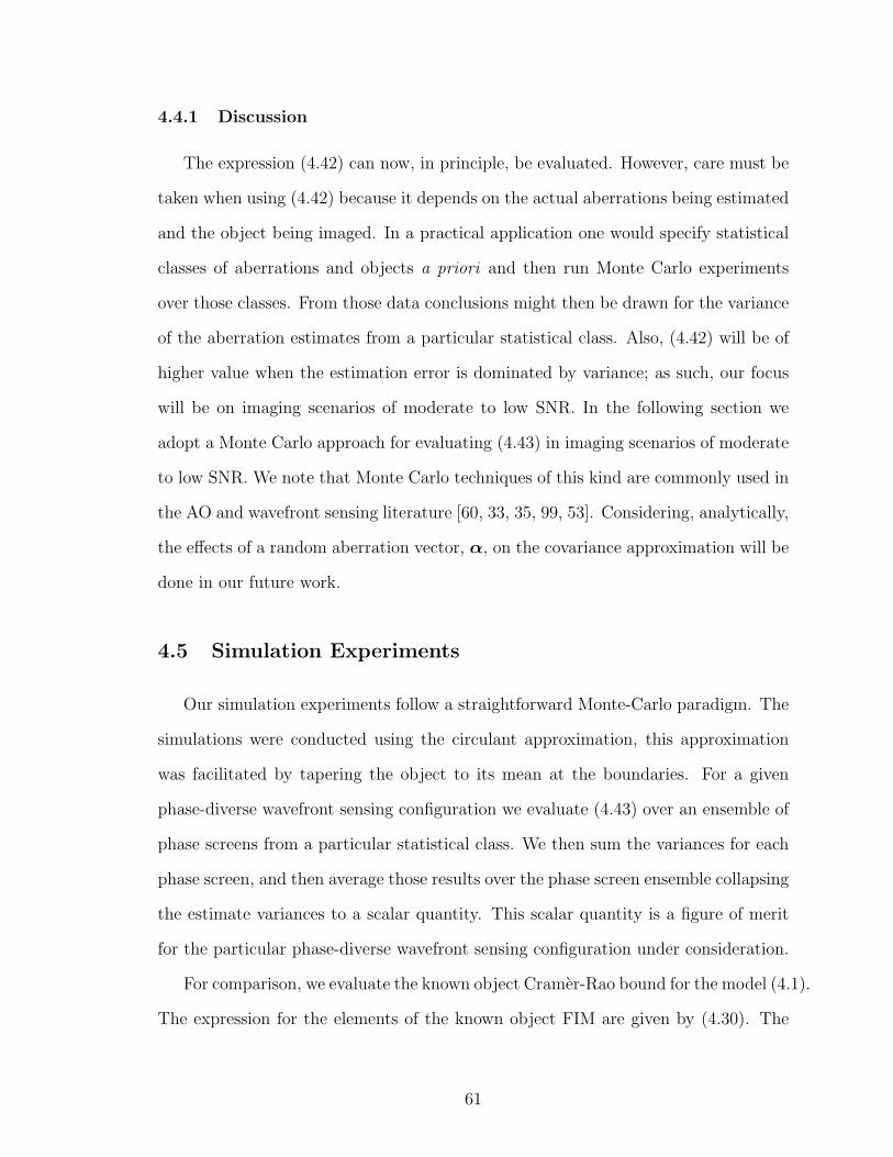
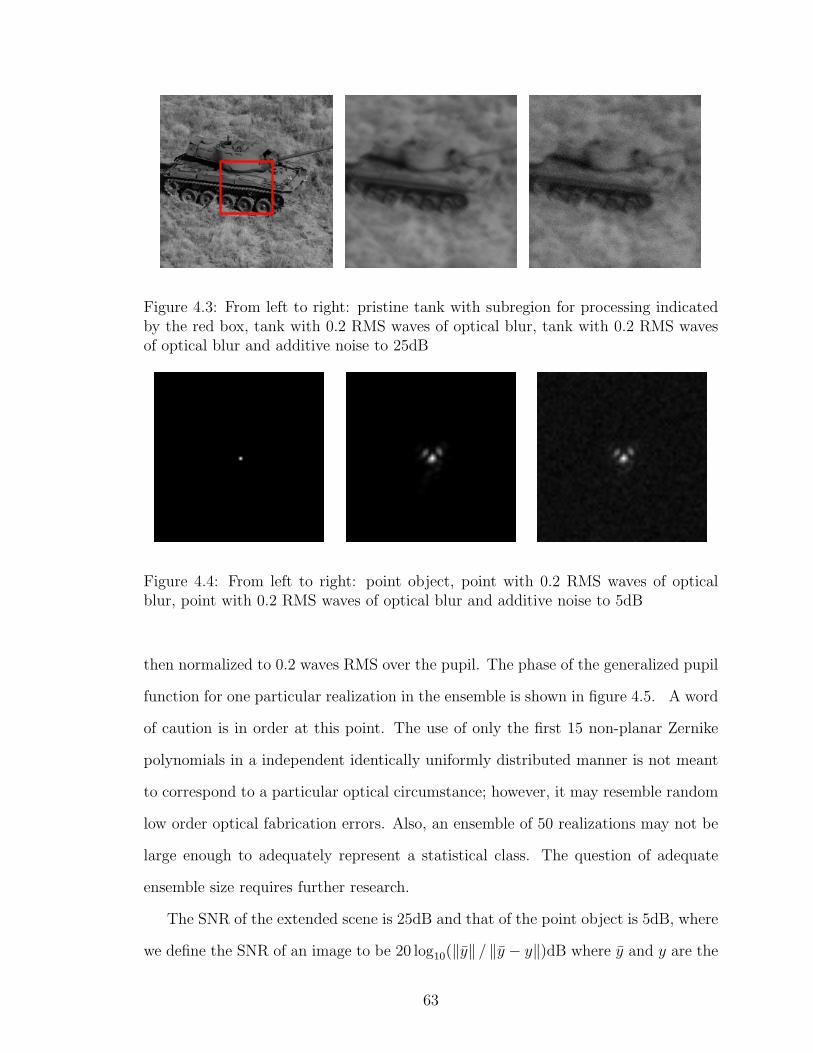
image, the subregion that is processed is indicated by a red box in figure 4.3; the point
object is also of size [64 × 64] pixels. The imagery is corrupted by space-invariant
blur and zero mean independent-identically-distributed additive Gaussian noise of
variance σ2. The objects, blurred objects, and blurry and noisy objects are shown in
figures 4.3 and 4.4.
In all of the calculations presented here the pupil phase aberrations were pa-
rameterized using Zernike polynomials 4 through 19 as defined in [60]; that is, the
expansion basis, ϕi, is composed of Zernike polynomials. Each phase screen re-
alization, in a 50 realization ensemble, was constructed by first drawing aberration
coefficients, α, from a uniform distribution over the interval [−1, 1] and using them
as weights in a basis expansion over an annular pupil. The resulting phase screen is
62
Figure 4.3: From left to right: pristine tank with subregion for processing indicatedby the red box, tank with 0.2 RMS waves of optical blur, tank with 0.2 RMS wavesof optical blur and additive noise to 25dB
Figure 4.4: From left to right: point object, point with 0.2 RMS waves of opticalblur, point with 0.2 RMS waves of optical blur and additive noise to 5dB
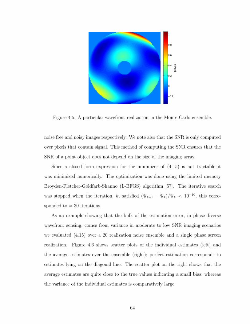
then normalized to 0.2 waves RMS over the pupil. The phase of the generalized pupil
function for one particular realization in the ensemble is shown in figure 4.5. A word
of caution is in order at this point. The use of only the first 15 non-planar Zernike
polynomials in a independent identically uniformly distributed manner is not meant
to correspond to a particular optical circumstance; however, it may resemble random
low order optical fabrication errors. Also, an ensemble of 50 realizations may not be
large enough to adequately represent a statistical class. The question of adequate
ensemble size requires further research.
The SNR of the extended scene is 25dB and that of the point object is 5dB, where
we define the SNR of an image to be 20 log10(‖y‖ / ‖y − y‖)dB where y and y are the
63
[wav
es]
−0.2
0
0.2
0.4
0.6
0.8
1
Figure 4.5: A particular wavefront realization in the Monte Carlo ensemble.
noise free and noisy images respectively. We note also that the SNR is only computed
over pixels that contain signal. This method of computing the SNR ensures that the
SNR of a point object does not depend on the size of the imaging array.
Since a closed form expression for the minimizer of (4.15) is not tractable it
was minimized numerically. The optimization was done using the limited memory
Broyden-Fletcher-Goldfarb-Shanno (L-BFGS) algorithm [57]. The iterative search
was stopped when the iteration, k, satisfied (Ψk+1 − Ψk)/Ψk < 10−10, this corre-
sponded to ≈ 30 iterations.
As an example showing that the bulk of the estimation error, in phase-diverse
wavefront sensing, comes from variance in moderate to low SNR imaging scenarios
we evaluated (4.15) over a 20 realization noise ensemble and a single phase screen
realization. Figure 4.6 shows scatter plots of the individual estimates (left) and
the average estimates over the ensemble (right); perfect estimation corresponds to
estimates lying on the diagonal line. The scatter plot on the right shows that the
average estimates are quite close to the true values indicating a small bias; whereas
the variance of the individual estimates is comparatively large.
64
−0.6 −0.4 −0.2 0 0.2 0.4 0.6
−0.6
−0.4
−0.2
0
0.2
0.4
0.6
α
α e
stim
ates
−0.6 −0.4 −0.2 0 0.2 0.4 0.6
−0.6
−0.4
−0.2
0
0.2
0.4
0.6
α
aver
age
α e
stim
ate
Figure 4.6: Individual aberration estimates and averaged estimates.
The evaluation of (4.43) requires the selection of a regularization “tuning” param-
eter. Previous experience with phase diversity suggests that the aberration estimates
are weakly dependent on the regularization parameter provided the regularization is
small. We verify this claim by evaluating (4.43) over our phase screen ensemble for
several different regularization parameters. The resulting curve is shown in Fig. 4.7.
The curve shows that for regularization parameters smaller than approximately 10−6
the standard deviation of the estimates is nearly constant.
10−15
10−10
10−5
100
105
0.6
0.7
0.8
0.9
1
1.1
β
Nor
mal
ized
std
[wav
es]
Figure 4.7: Estimated standard deviation as a function of β.
65
4.6 Results and discussion
The results of our simulation experiments for selection of the defocus parameter
are summarized in table 4.1. Figure 4.8 shows comparisons of the average of the
estimate standard deviations using (4.43) and the known-object Cramer-Rao bound
using (4.30), as well as the RMSE of the Monte Carlo simulation, for the extended
scene over a range of defocus values. An immediate observation is that the Cramer-
Rao bound method is lower than the estimated standard deviations using (4.43).
This is consistent with intuition as the Cramer-Rao bound assumes complete knowl-
edge of the object and one would expect improved estimator performance under that
condition. Observe further that the minima of the two methods are different. The
Cramer-Rao bound method predicts an optimal defocus value of 1.30 waves whereas
equation (4.43) predicts an optimal defocus value of 1.75 waves. The Monte Carlo
simulations yield an optimal defocus of 2.20 waves. The predicted optimal defocus
value using approximation (4.43) is closer to the Monte Carlo result than that pre-
dicted by the known-object Cramer-Rao bound. This makes intuitive sense as (4.43)
incorporates the uncertainty in the object whereas the Cramer-Rao method does not.
Table 4.1: Predictions of optimal defocus strength using (4.43), (4.30), and (4.15)
Figure 4.9 shows comparisons of the average of the estimate variances using (4.43)
and (4.30), as well as the RMSE of the Monte Carlo simulation, for the point object
over a range of defocus values. As with the extended scene, the Cramer-Rao bound
is lower than the variance predicted by (4.43). We see also that the optimal defocus
66
0 0.5 1 1.5 2 2.5 3 3.5 410−4
10−3
10−2
10−1
100
waves of defocus
RM
SE [w
aves
]
var−approxknown−obj CRBmonte carlo
Figure 4.8: Comparison of the average of the estimate standard deviations calculatedvia both (4.43) and (4.30), as well as the RMSE of the Monte Carlo simulation, forthe extended scene.
values for the two methods are very nearly equal; the minimum for the Cramer-Rao
bound occurs at 0.85 waves and the minimum for equation (4.43) is at 0.95 waves.
The optimal defocus value for (4.15) occurs at 1.05 waves. Although the minima
for the three methods are very near one another we note that the minimum given
by (4.43) is closer to the minimum obtained through Monte Carlo simulations.
It is important to note that both the Cramer-Rao bound and the variance ap-
proximation (4.43) are useful as guides in system parameter selection; one would be
remiss to use either of these methods as a complete substitute for full simulation
using (4.15). The primary benefit of (4.43) is that it can provide reasonable bounds
on parameters of interest for far less computational expense than performing full
Monte Carlo simulations. The ratio of computation time, for a single realization and
a [64× 64] object, of (4.15) to (4.43) is ≈ 12; a sizable time savings.
67
0 0.5 1 1.5 2 2.5 310−4
10−3
10−2
10−1
100
waves of defocus
RM
SE [w
aves
]
var−approxknown−obj CRBmonte carlo
Figure 4.9: Comparison of the average of the estimate standard deviations calculatedvia both (4.43) and (4.30), as well as the RMSE of the Monte Carlo simulation, forthe point object.
68
4.7 Conclusion and future work
A method for approximating the variance of aberration estimates for quadratically
regularized weighted least squares estimators in the phase diversity context have
been presented. The approximation has been shown to be a fairly accurate guide in
selecting an appropriate amount of defocus for the diversity channel. The benefit of
using (4.43) over (4.30) is delineated when the object is an extended scene; however
the two methods do not differ substantially when the object is a point source.
The next steps in this research are to explore approximations to the bias of (4.15).
An approximation to the bias could be used with (4.43) to approximate the entire
mean squared error for aberration estimation. These expressions could also be used
to explore how regularization of the object affects the aberration estimates. A natural
next step is also to investigate why the known-object Cramer-Rao bound differs from
the approximation (4.43) less for point objects than for extended scenes.
69
CHAPTER V
Conclusion and future work
5.1 Summary
In this dissertation we have analyzed penalized-likehood estimation techniques
for polarimetric imagery. We have explored the question of which space is the ap-
propriate space to estimate in: intensity space or Stokes space. It was found that
estimation of Stokes vectors directly provides estimates with lower overall RMS er-
ror as compared with restoring the intensity images and then transforming to Stokes
space for interpretation. We have also explored how the addition of a cross-channel
regularization term affects estimation accuracy. It was found that the addition of a
cross-channel regularization term improves interpretability of Stokes parameter esti-
mates when estimating the Stokes parameters directly and when using a traditional
estimator.
While the addition of a cross-channel regularization term has improved inter-
pretability for both estimators it has also added another set of regularization “tuning”
parameters. For practical implementation the added computation cost of additional
regularization penalty functions should be considered. The proposed Stokes space
estimator has been shown to provide lower RMS reconstruction errors, however, the
traditional estimator has only one tuning parameter to be adjusted as opposed to the
Stokes estimator which has three. Further study into the computational cost verses
70
reconstruction error between the proposed estimator and the traditional estimator is
warranted for implementation decisions.
We have also developed a unified framework for joint estimation of Stokes images
and aberrations from polarimetric measurements that contain phase diversity. We
explored two methods, (3.18) and (3.22), for joint estimation of Stokes images and
aberrations. It was found that estimation accuracy follows a task-based hierarchy,
i.e., in a joint-estimation framework the choice of algorithm is task dependent. When
the task is image restoration (aberrations are nuisance parameters) an algorithm that
jointly estimates object and aberrations while incorporating a priori knowledge of
the object is appropriate. However, if the aberration parameters are of interest and
the object is a nuisance parameter then a reduced-parameter algorithm should be
chosen.
The magnitudes of the regularization tuning parameters are very different depend-
ing on which parameters are of importance. When the aberration parameters are of
interest and the object is nuisance the regularization parameter is quite small and the
estimates are weakly dependent on the parameter over a wide range of values. In the
limit as the regularization parameter approaches zero (3.22) becomes a maximum-
likelihood estimator (that cannot be evaluated for circular apertures). It seems then,
that the primary role of regularization in (3.22) is to ensure invertibility of the matrix
in (3.21).
We have developed of a method for approximating the variance of aberration
estimates for quadratically penalized weighted least squares estimators in the phase
diversity context. Comparisons for system-parameter selection were made between
the commonly used known-object Cramer-Rao bound and our variance approximation
that takes into account an unknown object. The impact including the uncertainty
of the object in the formulation has been shown to be significant when selecting the
diversity defocus parameter when imaging extended scenes. When imaging a point
71
object the known-object Cramer-Rao bound yields a minimum variance defocus value
nearly equal to our approximation that incorporates the uncertainty in the object.
From a practical point of view our approximation to the variance has significant
utility; evaluation of the variance approximation (4.43) for 15 aberration parameters
is 12 times faster than a single evaluation of (4.15).
5.2 Future Work
While this dissertation has focused primarily on polarimetric image reconstruction
algorithms the framework is general and may be applied to other imaging modali-
ties. The framework developed may be immediately applied to any imaging modality
where there is a linear relationship between the estimation space and measurement
space. An example of this is multi/hyper-spectral imaging. Spectral measurements
are made using optical filters that pass a range of wavelengths. Real scenes under so-
lar illumination contain information across a continuum of wavelengths, each spectral
measurement is a sum of contributions from different wavelengths. In the polarimet-
ric case our linear transformation TJ×3 specified J ≥ 3, but with spectral imaging we
have TJ×K where K ≥ J . A model of this type highlights the possibility of estimating
fine spectral components from measurements that are coarsely sampled in wavelength.
This could be used, for example, for detection of materials with narrow spectral sig-
natures. For example, a typical multispectral imager may have four spectral bands
each with bandwidths of λ/5 where λ is the mean wavelength of a particular band. In
our proposed framework one could estimate spectral bands with bandwidths of λ/10
thereby effectively increasing the spectral resolution of the imager. Consequently,
there is the potential to detect finer spectral signatures. Moreover, improvement in
detection of fine spectral signatures is a motivation for regularization design.
There are subtleties that have to be addressed when applying these methods to
spectral imaging. The wavelength dependence of the point-spread-function as well as
72
the sample rate at the detector should be modeled appropriately. Research into the
impact of aliasing, due to wavelength variation, is of practical importance for spectral
imager design. Also, regularization strategies for recovery of aliased information in
the spectral imaging context has yet to be explored.
A more general extension of the Stokes estimation framework would be to con-
sider estimation spaces that are nonlinearly related to the measurements. Some re-
lated work has been done already in the area spectral anomaly detection [51, 50, 76].
However, development of image reconstruction algorithms in this area has received
little attention. Exploration of penalized-likelihood estimators that perform estima-
tion in a space that is nonlinearly related to the measurements offers the potential for
dimensionality reduction opens up new motivations for regularization penalty design.
All of the algorithms in this work have assumed a monochromatic object, in re-
ality the world polychromatic. These algorithms can be generalized to accommodate
polychromatic objects. There are two areas where the polychromatic nature of light
will enter: (1) point-spread function, and (2) detector sampling. The PSF scales with
wavelength to first order so that can be dealt with in a straightforward manner; the
detector sampling also scales with wavelength but one must be mindful of aliasing
effects at the blue end of the spectrum.
The polarimetric-phase-diverse wavefront sensing algorithm (4.15) can be explored
further by switching paradigms to a Bayesian framework. In the Bayesian frame work
the regularization penalty is viewed as a statistical prior on the object. In our frame-
work the only requirement on our quadratic regularization penalty was that C′C
be positive definite. Using Parseval’s theorem (3.22) can be written in the Fourier
domain. In the Bayesian paradigm, in the Fourier domain, the regularization penalty
now takes on the meaning of the inverse power-spectral density of the object. For
extended scenes different object PSDs can be explored. For example, an image of
Manhattan, New York, will have strong spatial frequencies corresponding to the grid-
73
like street structure of the city, whereas farm land may not exhibit any preferential
direction in the frequency domain.
It would be natural to extend the expression for the approximate joint covari-
ance matrix to include other system parameters. For example, in this dissertation we
have assumed that the measurements were all perfectly registered and sampled at the
Nyquist rate, however, this is seldom the case for real phase-diversity systems. Gen-
eralization of (4.43) to include multiple system parameters would provide a means
for studying the effects of channel misregistration, aliasing, or other system param-
eters on wavefront estimation. Similarly, in our polarimetric work we have assumed
the polarimetric channels were perfectly aligned and sampled at the Nyquist rate.
Again, a generalization of (4.43) to polarimetric-phase-diverse systems would provide
a starting point for analyzing how system nonidealities effect wavefront estimation.
Analytical analysis of our covariance approximation under the consideration of a
random α is forthcoming. To complement this we plan to compare variations of our
analytic predictions over an aberration ensemble with the variations of the Monte
Carlo simulations over the same ensemble. Moreover, we plan to tailor the aberra-
tion ensemble to more accurately represent atmospheric turbulence using Kolmogorov
statistics.
In our joint estimation of object and aberrations we have found that one can either
have better object estimates or better aberration estimates but not both. We plan to
thoroughly investigate joint estimation versus staged estimation. Intuitively it seems
that the full joint model would give the best estimates for object and aberration but
it is not clear that this is the case and it deserves further attention.
Further analysis of phase-diverse wavefront sensor performance would benefit from
an expression for the approximate bias of the aberration estimates. This calculation
involves a third order Taylor expansion of an implicit estimator[29] and so simpli-
fying assumptions seem imperative. However, once armed with approximations for
74
the covariance and bias of the aberrations estimates it would be of great utility in
analyzing how regularization of the object or aberrations, affects the estimation of
the aberration parameters. That is, one could analyze the effect of a statistical prior
on the aberrations in addition to the object regularization.
As mentioned above, higher fidelity system models are practical importance. Ap-
proximations for the covariance and bias of (4.15) can be generalized to accommo-
date registration parameters, channel transmission, pixel aggregation, etc. That
is, if the joint parameter to be estimated, Θ, consists of L types of parameters,
Θ = (θ1, . . . ,θL), that enter into the estimation problem both linearly and nonlin-
early, one could analyze their joint impact on reconstruction quality using approxi-
mations to the bias and covariance.
In appendix B we demonstrated graphically, for a three-channel polarimeter, that
the set of angles θi = π(i−1)J
for i = 1, . . . , J was an optimal in the Cramer-Rao
sense. We also conjectured that the same set of angles would be optimal for a J-
channel polarimeter and showed that those angles are indeed an extreme point of
the J-channel objective function. A path forward for proving that the set of angles
is indeed a minimum variance set includes showing that the set of angels is a local
minimum and not a maximum. This can be accomplished by showing that the Hessian
evaluated at the prescribed set is positive definite. The next, more difficult step, is
to show that the angles are a global minimum and not a local minimum. A second
approach would be to explore a single-value decomposition of the FIM . The FIM
has a large amount of structure and so may have a “nice” SVD. Once the SVD
is in hand one can use the fact that the trace is similarity invariant and obtain the
inverse without too much difficulty. From there one could work towards a closed-form
expression for the minimizing set of angles.
75
APPENDICES
76
APPENDIX A
Numerical minimization of (3.22)
Numerical minimization of equation (3.22)
The minimization of (3.22) is most easily accomplished by invoking Parseval’s
theorem. If we ignore inconsequential constants our objective function can be written
in the Fourier domain as
Φ(α) =1
2
J∑j=1
∥∥Yj −ΩjΛjΘ(α)∥∥2
+1
2
2∑n=0
βn∥∥DΘn(α)
∥∥2, (A.1)
where Yj = Q′yj, Λj = [TJ×3](j,1:3) ⊗ Inp , Θ(α) = Q′S(α), Ω(α) = Q′B(α), and D
is a matrix such that D′D = QCC′Q′. The partial derivatives of (A.1) with respect
to the ith aberration parameter can be written
∂Φ∂αi
= −12
J∑j=1
⟨∂Ωj
∂αiΛjΘ + ΩjΛj
∂Θ∂αi
, Yj −ΩjΛjΘ⟩
+12
2∑n=0
βn
⟨D∂Θn
∂αi, DΘn
⟩+ c.c,
where the dependencies on αi have been suppressed for brevity, 〈· , ·〉 is the Eu-
clidean inner product over C3np , and c.c denotes complex conjugate. To evaluate this
expression, the partial derivatives of Ωj and Θ(α) must be calculated.
77
Expression for ∂Θ∂αi
Recall, equation (3.21) expresses the Stokes parameters in terms of the aberration
parameters:
S(α) =
(T′J×3 ⊗ Inp
)B (α)′B (α)
(TJ×3 ⊗ Inp
)+ σ2β3 ⊗C′C︸ ︷︷ ︸
P
−1
×(T′J×3 ⊗ Inp
)B (α)′ y︸ ︷︷ ︸
V
.
(A.2)
This expression may be written as a matrix-vector product: S(α) = P−1(α;β3)V(α; y),
and a similar expression may be written in the Fourier domain
Θ(α) = A−1(α;β3)X(α; Y). (A.3)
The partial derivative of (A.1) with respect to αi is then
∂Θ
∂αi=
∂
∂αi
(A−1X
)=∂A−1
∂αiX + A−1 ∂X
∂αi(A.4)
= −A−1 ∂A
∂αiA−1X + A−1 ∂X
∂αi(A.5)
= −A−1
(2
J∑j=1
[TJ×3]′j[TJ×3]j ⊗ Re
Ω′j
∂Ωj
∂αi
)A−1
J∑j=1
Λ′jΩ′jYj
+ A−1
J∑j=1
Λ′j∂Ω′j∂αi
Yj
. (A.6)
With this expression in place it remains to write down an expression for A−1 and
compute the partial derivatives of Ωj with respect to αi.
78
Expression for∂Ωj
∂αi
∂
∂αiΩj =
∂
∂αic F
[∣∣F−1 [Pj]∣∣2] (A.7)
= c F
[∂
∂αi
∣∣F−1 [Pj]∣∣2] (A.8)
= 2c F
[Re
(F−1
[∂Pj∂αi
]) (F−1 [Pj]
)∗](A.9)
= 2c F[Re(
F−1 [ıψiPj]) (
F−1 [Pj])∗]
(A.10)
= 2c F[−Im
(F−1 [ψiPj]
) (F−1 [Pj]
)∗](A.11)
= 2c F[ImF−1 [Pj]
(F−1 [ψiPj]
)∗], (A.12)
where c normalizes the PSF to unit volume.
79
Expression for A−1 for the case of polarization angles 0, 45, 90, 135
For a J channel polarimeter the matrix A has a (3 × 3) block structure and so
can be inverted by hand. For our specific case, the expression for A−1 can be written
as horizontally concatenated (3× 1) block-column vectors in the following way:
A−1 =1
16 det [A]
(∣∣Ω1
∣∣2 +∣∣Ω3
∣∣2 + 4β1
∣∣D∣∣2)(∣∣Ω2
∣∣2 +∣∣Ω4
∣∣2 + 4β2
∣∣D∣∣2)−(∣∣Ω1
∣∣2 − ∣∣Ω3
∣∣2)(∣∣Ω2
∣∣2 +∣∣Ω4
∣∣2 + 4β2
∣∣D∣∣2)−(∣∣Ω2
∣∣2 − ∣∣Ω4
∣∣2)(∣∣Ω1
∣∣2 +∣∣Ω3
∣∣2 + 4β1
∣∣D∣∣2)
−(∣∣Ω1
∣∣2 − ∣∣Ω3
∣∣2)(∣∣Ω2
∣∣2 +∣∣Ω4
∣∣2 + 4β2
∣∣D∣∣2)(∑4j=1
∣∣Ωj
∣∣2 + 4β0
∣∣D∣∣2)(∣∣Ω2
∣∣2 +∣∣Ω4
∣∣2 + 4β2
∣∣D∣∣2)− (∣∣Ω2
∣∣2 − ∣∣Ω4
∣∣2)2
(∣∣Ω1
∣∣2 − ∣∣Ω3
∣∣2)(∣∣Ω2
∣∣2 − ∣∣Ω4
∣∣2)
−(∣∣Ω2
∣∣2 − ∣∣Ω4
∣∣2)(∣∣Ω1
∣∣2 +∣∣Ω3
∣∣2 + 4β1
∣∣D∣∣2)(∣∣Ω1
∣∣2 − ∣∣Ω3
∣∣2)(∣∣Ω2
∣∣2 − ∣∣Ω4
∣∣2)(∑4j=1
∣∣Ωj
∣∣2 + 4β0
∣∣D∣∣2)(∣∣Ω1
∣∣2 +∣∣Ω3
∣∣2 + 4β1
∣∣D∣∣2)− (∣∣Ω1
∣∣2 − ∣∣Ω3
∣∣2)2
,
where
64 det[A] =
4∑j=1
∣∣Ωj
∣∣2 + 4β0
∣∣D∣∣2(∣∣Ω1
∣∣2 +∣∣Ω3
∣∣2 + 4β1
∣∣D∣∣2)(∣∣Ω2
∣∣2 +∣∣Ω4
∣∣2 + 4β2
∣∣D∣∣2)
−(∣∣Ω2
∣∣2 − ∣∣Ω4
∣∣2)2 (∣∣Ω1
∣∣2 +∣∣Ω3
∣∣2 + 4β1
∣∣D∣∣2)−(∣∣Ω1
∣∣2 − ∣∣Ω3
∣∣2)2 (∣∣Ω2
∣∣2 +∣∣Ω4
∣∣2 + 4β2
∣∣D∣∣2) .With the component expressions for the partial derivatives for the reduced-parameter
objective function in place gradient-based search methods may be used. It is worthy
to note that search methods that do not use gradient information are futile for the
objective function (3.22). We examined the standard derivative-free simplex method
(the MATLAB fminsearch algorithm) and found that reaching the global minimum
of (3.22) would take more than 3 days of computation whereas the gradient-based
L-BFGS method requires less than 20 minutes to reach the global minimum.
80
APPENDIX B
Optimal angles for a three-channel linear
polarimeter
Optimal angles for a three-channel polarimeter
In this appendix we use the Cramer-Rao bound as a metric for determining the
optimal polarization angles for a three-channel linear polarimeter; we also provide a
conjecture for a set of optimal polarization angles for J-channel linear polarimeter.
Consider the following model for a J-channel linear polarimeter
y = (TJ×3 ⊗ Inp)S + ε, (B.1)
where,
TJ×3 =
12
12
cos(2θ1) 12
sin(2θ1)
12
12
cos(2θ2) 12
sin(2θ2)
......
...
12
12
cos(2θJ) 12
sin(2θJ)
(B.2)
This model ignores the effects of optical blur as polarization is independent of phase
in the visible regime. Under the noise model ε ∼ N(0, σ2Inp) we may write down the
81
following log-likelihood function
L(S;θ) =1
2
∥∥y − (T′J×3(θ)TJ×3(θ)⊗ Inp)S∥∥2, (B.3)
where θ = (θ1, . . . , θJ). The Fisher-Information Matrix (FIM ) for (B.3) is given by
F = T′J×3(θ)TJ×3(θ)⊗ Inp . (B.4)
At this point we may consider the FIM as a function of θ. The variances in the
estimates of the Stokes parameters are then a function of the polarizer angles and are
equal to the diagonal elements of the inverse FIM :
F−1 =[T′J×3(θ)TJ×3(θ)
]−1 ⊗ Inp , (B.5)
where
T′J×3(θ)TJ×3(θ) =
∑J
ı=114
∑Jı=1
14
cos(2θı)∑J
ı=114
sin(2θı)∑Jı=1
14
cos(2θı)∑J
ı=114
cos2(2θı)∑J
ı=118
sin(4θı)∑Jı=1
14
sin(2θı)∑J
ı=118
sin(4θı)∑J
ı=114
sin2(2θı)
. (B.6)
The inverse of any invertible 3× 3 matrix F is written
F−1 =1
det(F)
F22F33 − F2
23 F13F32 − F12F33 F12F23 − F13F22
F23F31 − F21F33 F11F33 − F213 F13F21 − F11F23
F21F32 − F22F31 F12F31 − F11F32 F11F22 − F212
. (B.7)
We define our performance metric to be the trace of the FIM :
θ = argminθ
= Tr[F−1(θ)]4= Ψ(θ). (B.8)
82
Without loss of generality we can set θ1 = 0. Now, specializing to three channels we
have θ = (θ2, θ3). The objective function Ψ(θ2, θ3) becomes
Ψ(θ2, θ3) = −1
8
4 cos (2θ2) + cos (4θ2) + 4 cos (2 (θ2 − θ3)) + cos (4 (θ2 − θ3))
sin2 (θ2) sin2 (θ2 − θ3) sin2 (θ3)
+4 cos (2θ3) + cos (4θ3)− 15
sin2 (θ2) sin2 (θ2 − θ3) sin2 (θ3)
(B.9)
Figures B.1 and B.2 show density plots of log[Ψ(θ2, θ3)] θ2, θ3 ∈ (0, π); figure B.2
has been thresholded at log(25) for better color representation. Observe that there
0 Π
3
2 Π
3
Π
0
Π
3
2 Π
3
Π
Θ2
Θ3
2
3
4
5
6
7
8
9
Figure B.1: Density plot of log(Ψ).
are two convex regions separated by the line θ2 = θ3. If we demand that the angles are
ordered in a monotonically increasing fashion, the valid solution space lies above the
line θ2 = θ3. We solve (B.8) numerically using a constrained Nelder-Meade numerical
optimization routine. The results of the search are
θ2 → 1.0471975511966241732
θ3 → 2.0943951023933713478.
83
0 Π
3
2 Π
3
Π
0
Π
3
2 Π
3
Π
Θ2
Θ3
1.8
2.0
2.2
2.4
2.6
2.8
3.0
3.2
Figure B.2: Density plot of log(Ψ) thresholded for enhanced color representation.
These numbers are suspiciously close to π/3 and 2π/3 respectively. Although (B.9)
does not appear to lend itself to an analytic minimum, we can evaluate the gradient of
our objective function at the intuitive solution of (π/3, 2π/3). If the gradient vanishes
we conjecture that (π/3, 2π/3) is the global minimum. The partial derivatives of (B.9)
are
∂Ψ
∂θ2
=sin (2θ2 − 5θ3) + sin (4θ2 − 5θ3) + 4 sin (2θ2 − 3θ3) + 3 sin (4θ2 − 3θ3)
8 sin3 (θ2) sin3 (θ2 − θ3) sin2 (θ3)
+−26 sin (2θ2 − θ3) + 3 sin (4θ2 − θ3) + 4 sin (2θ2 + θ3)
8 sin3 (θ2) sin3 (θ2 − θ3) sin2 (θ3)
+sin (4θ2 + θ3) + sin (2θ2 + 3θ3)
8 sin3 (θ2) sin3 (θ2 − θ3) sin2 (θ3)
(B.10)
∂Ψ
∂θ3
=4 cos (θ2) sin (2 (θ2 − 2θ3)) cot2 (θ2)
4 sin3 (θ2 − θ3) sin3 (θ3)
+(4 cos (2θ2) cos (4θ2)− 13) csc2 (θ2) sin (θ2 − 2θ3)
4 sin3 (θ2 − θ3) sin3 (θ3).
(B.11)
Evaluation the partial derivatives at (π/3, 2π/3) verifies that indeed the gradient of
the objective vanishes.
84
Conjecture
We conjecture that a set of minimum-variance angles, in the Crame-Rao sense,
for a J-channel linear polarimeter is θl = π l−1J for l = 1, . . . , J . We show next
that this set of angles is an extreme point of Ψ(θ). The diagonal elements of the
J-channel inverse FIM can be written as a ratio of functions, f(θ)/g(θ):
[F−1](1,1) =f1(θ)
g(θ), [F−1](2,2) =
f2(θ)
g(θ), [F−1](3,3) =
f3(θ)
g(θ), (B.12)
where the functions have been defined to be consistent with (B.7). Consider the
derivative of our metric with respect to the lth component of θ:
∂
∂θlTr[F−1] =
∂
∂θl
f1(θ) + f2(θ) + f3(θ)
g(θ)(B.13)
The general form of the first derivative of a ratio of functions is given by the quotient
rule (f(θ)
g(θ)
)′=f ′(θ)g(θ)− g′(θ)f(θ)
g(θ)2, (B.14)
this function vanishes if f ′(θ) and g′(θ) are both zero (g(θ) is nonzero by assumption).
We will differentiate each term in the numerator and show that the resulting sum
is zero for the conjectured set of angles, we will then differentiate the denominator
85
and show that it vanishes for the same set of angles.
∂f1
∂θl=
∂
∂θl
(F22F33 − F2
23))
(B.15)
=∂
∂θl
(J∑ı=1
1
4cos2(2θı)
)(J∑=1
1
4sin2(2θ)
)− ∂
∂θl
(J∑k=1
1
8sin(4θk)
)2
(B.16)
=
(cos(2θl) sin(2θl))
((J∑ı=1
1
4cos2(2θı)
)−
(J∑=1
1
4sin2(2θ)
))
− cos(4θl)J∑k=1
1
8sin(4θk)
. (B.17)
We evaluate (B.17) by invoking the following trigonometric identities
J∑ı=1
cos2(Lπı− 1
J) =
J∑ı=1
sin2(Lπı− 1
J) =
J
2, L = even (B.18)
J∑k=1
cos(Lπk − 1
J) =
J∑k=1
sin(Lπk − 1
J) = 0, L = even, (B.19)
using these in (B.17) yields
∂f1
∂θl= (1/4) cos(2π
l − 1
J) sin(2π
l − 1
J)(J
2− J
2)− (1/8) cos(4π
l − 1
J)(0) = 0. (B.20)
Continuing with the next two terms we have
∂f2
∂θl=
∂
∂θl
(F11F33 − F2
13))
(B.21)
=J
4
∂
∂θl
J∑=1
1
4sin2(2θ)−
∂
∂θl
(J∑k=1
1
4sin(2θk)
)2
(B.22)
=J
4cos(2θl) sin(2θl)−
1
4cos(2θl)
J∑k=1
1
4sin(2θk), (B.23)
86
evaluation over the prescribed set yields
∂f2
∂θl=J
4cos
(2πl − 1
J
)sin
(2πl − 1
J
). (B.24)
The third term is
∂f3
∂θl=
∂
∂θl
(F11F22 − F2
12))
(B.25)
=J
4
∂
∂θl
J∑ı=1
1
4cos2(2θı)−
∂
∂θl
(J∑k=1
1
4cos(2θk)
)2
(B.26)
= −J4
cos(2θl) sin(2θl)−1
4sin(2θl)
J∑k=1
1
4sin(2θk), (B.27)
evaluation over the prescribed set yields
∂f3
∂θl= −J
4cos
(2πl − 1
J
)sin
(2πl − 1
J
). (B.28)
Putting the three terms together we have
∂(f1 + f2 + f3)
∂θl
∣∣∣∣θl=π(l−1)/J
= 0, (B.29)
since this expression is independent of l, it holds for all components of θ. It remains
to show that ∂∂θlg(θ)
∣∣θl
= 0, l = 1, . . . , J .
Recall, g(θ) = det(F). We will use the following identity in our work:
∂ det(F)
∂θ= det (F) Tr
(F−1∂F
∂θ
). (B.30)
Equation (B.30) vanishes if Tr(
F−1 ∂F∂θl
)= 0. We now write out the elements of the
87
trace [F−1 ∂F
∂θl
]11
=(F22F33 − F2
23
) ∂F11
∂θl
+ (F13F32 − F12F33)∂F21
∂θl
+ (F12F23 − F13F22)∂F31
∂θl
, (B.31)
[F−1 ∂F
∂θl
]22
= (F23F31 − F21F33)∂F12
∂θl
+(F11F33 − F2
13
) ∂F22
∂θl
+ (F13F21 − F11F23)∂F32
∂θl
, (B.32)
[F−1 ∂F
∂θl
]33
= (F21F32 − F22F31)∂F13
∂θl
+ (F12F31 − F11F32)∂F23
∂θl
+(F11F22 − F2
12
) ∂F33
∂θl
. (B.33)
Each of these expressions must be evaluated at θl = π l−1J
. Consider (B.31); the first
term is zero due to F11 being independent of angle, the second and third terms also
vanish since F12
∣∣θl=π
l−1J
= F13
∣∣θl=π
l−1J
= 0. Equation (B.32) has two vanishing terms
since F23
∣∣θl=π
l−1J
= 0 as well. Lastly, using the previous identities, equation (B.32)
also has two vanishing terms. There are two nonzero terms left in the trace:
Tr(
F−1 ∂F∂θl
) ∣∣∣∣θl=π
l−1J
=[(
F11F33 − F213
) ∂F22
∂θl+(F11F22 − F2
12
) ∂F33
∂θl
] ∣∣∣∣θl=π
l−1J
. (B.34)
Observe that ∂F22
∂θl= −∂F33
∂θl, F12
∣∣θl=π
l−1J
= F12
∣∣θl=π
l−1J
= 0, and that F22
∣∣θl=π
l−1J
=
88
F33
∣∣θl=π
l−1J
= J8. Putting these together we have
Tr
(F−1 ∂F
∂θl
) ∣∣∣∣θl=π
l−1J
=J2
16− J2
16= 0. (B.35)
It has been demonstrated that the set polarization angles θl = π l−1J l = 1, . . . , J
is an extreme point of Ψ. Further research is needed to prove that the set of angles
θl = π l−1J l = 1, . . . , J is a global minimum of Ψ.
89
BIBLIOGRAPHY
90
BIBLIOGRAPHY
[1] S. Ahn and R.M. Leahy. Analysis of resolution and noise properties of non-quadratically regularized image reconstruction methods for PET. IEEE Trans-actions on Medical Imaging, 27(3):413, 2008.
[2] S. Ainouz, J. Zallat, A. de Martino, and C. Collet. Physical interpretation ofpolarization-encoded images by color preview. Optics express, 14:5916–5927,2006.
[3] A. Ambirajan and D.C. Look Jr. Optimum angles for a polarimeter: part I(Journal Paper). Optical Engineering, 34(06):1651–1655, 1995.
[4] A. Ambirajan and D.C. Look Jr. Optimum angles for a polarimeter: part I(Journal Paper). Optical Engineering, 34(06):1656–1658, 1995.
[5] I.B. Ayed, A. Mitiche, and Z. Belhadj. Polarimetric image segmentation viamaximum-likelihood approximation and efficient multiphase level-sets. IEEEtransactions on pattern analysis and machine intelligence, 28(9):1493, 2006.
[6] L. Bar, A. Brook, N. Sochen, and N. Kiryati. Deblurring of color images cor-rupted by impulsive noise. IEEE Transactions on Image Processing, 16(4):1101,2007.
[7] H.H. Barrett, K.J. Myers, and S. Dhurjaty. Foundations of image science.Journal of Electronic Imaging, 14:029901, 2005.
[8] J.D. Barter, H.R. Thompson, and C.L. Richardson. Visible-regime polarimetricimager: a fully polarimetric, real-time imaging system. Appl. Opt, 42:1620–1628, 2003.
[9] I. Berezhnyy and A. Dogariu. Polarimetric description of superposing randomelectromagnetic fields with different spectral composition. Journal of the OpticalSociety of America A, 21(2):218–222, 2004.
[10] A. Blanc, L.M. Mugnier, and J. Idier. Marginal estimation of aberrations andimage restoration by use of phase diversity. Journal of the Optical Society ofAmerica A, 20(6):1035–1045, 2003.
[11] P. Blomgren and T.F. Chan. Color TV: total variation methods for restorationof vector-valued images. IEEE Transactions on Image Processing, 7(3):304–309,1998.
91
[12] M.R. Bolcar and J.R. Fienup. Method of phase diversity in multi-aperturesystems utilizing individual sub-aperture control. In Proc. SPIE, volume 5896,pages 126–133, 2005.
[13] M.R. Bolcar and J.R. Fienup. Sub-aperture piston phase diversity for segmentedand multi-aperture systems. Applied Optics, 48(1):5–12, 2009.
[14] T.F. Chan and C.K.T. Wong. Multichannel image deconvolution by total vari-ation regularization. In Proceedings of SPIE, volume 3162, page 358, 1997.
[15] R.A. Chipman. ”Polarimetry” in Handbook of Optics, volume 2. McGraw-Hill,2 edition, 1995.
[16] G. Cincotti. Polarization gratings: design and applications. IEEE Journal ofQuantum Electronics, 39(12):1645–1652, 2003.
[17] F. Cremer, W. De Jong, and K. Schutte. Processing of polarimetric infraredimages for landmine detection. In 2nd International Workshop on AdvancedGround Penetrating Radar (IWAGPR. Citeseer, 2003.
[18] B.H. Dean, D.L. Aronstein, J.S. Smith, R. Shiri, and D.S. Acton. Phase re-trieval algorithm for JWST flight and testbed telescope. In Proceedings of SPIE,volume 6265, page 626511, 2006.
[19] B.H. Dean and C.W. Bowers. Diversity selection for phase-diverse phase re-trieval. Journal of the Optical Society of America A, 20(8):1490–1504, 2003.
[20] J.J. Dolne and H.B. Schall. Information theoretic bounds of phase diversityfor diversity polynomials and noise statistics. In Proceedings of SPIE, volume5553, page 127, 2004.
[21] J.J. Dolne and H.B. Schall. Cramer-Rao bound and phase-diversity blind decon-volution performance versus diversity polynomials. Applied optics, 44(29):6220–6227, 2005.
[22] J.J. Dolne and H.B. Schall. Fundamental performance bounds of phase diversityblind deconvolution algorithm for various diversity polynomials, noise statistics,and scene size. In Atmospheric Propagation II. Edited by Young, Cynthia Y.;Gilbreath, G. Charmaine. Proceedings of the SPIE, volume 5793, pages 118–128,2005.
[23] M.J. Duggin. Factors controlling discrimination in imaging polarimetry. InProceedings of SPIE, volume 5432, page 43. Citeseer, 2004.
[24] M.J. Duggin. Factors controlling the manual and automated extraction of imageinformation using imaging polarimetry. In Proceedings of SPIE, volume 5432,page 85. Citeseer, 2004.
92
[25] M.J. Duggin and R. Loe. Algorithms for target discrimination and contrastenhancement using narrowband polarimetric image data. In Proc. SPIE, volume4481. Citeseer, 2002.
[26] W.G. Egan. Polarization and surface roughness. In Proceedings of SPIE, volume3426, page 144, 1998.
[27] YC Eldar. Uniformly improving the Cramer-Rao bound and maximum-likelihood estimation. IEEE Transactions on Signal Processing, 54(8):2943–2956, 2006.
[28] H.W. Engl, M. Hanke, and A. Neubauer. Regularization of inverse problems.Kluwer Academic Pub, 1996.
[29] J.A. Fessler. Mean and variance of implicitly defined biased estimators (suchaspenalized maximum likelihood): applications to tomography. IEEE Transac-tions on Image Processing, 5(3):493–506, 1996.
[30] J.A. Fessler. Image Reconstruction: Algorithms and Analysis. TBD, TBD.
[31] J.A. Fessler and W.L. Rogers. Spatial resolution properties of penalized-likelihood image reconstruction: Space-invariant tomographs. IEEE Transac-tions on Image processing, 5(9):1346–1358, 1996.
[32] J. R. Fienup, J. C. Marron, T. J. Schulz, and J. H. Seldin. Hubble spacetelescope characterized by using phase-retrieval algoritihms. Applied Optics,32:1747–1768, 1993.
[33] JR Fienup, JC Marron, TJ Schulz, and JH Seldin. Hubble Space Telescopecharacterized by using phase-retrieval algorithms. Applied Optics, 32(10):1747–1767, 1993.
[34] B. Formwalt and S. Cain. Optimized phase screen modeling for optical turbu-lence. Appl. Opt, 45:5657–5668, 2006.
[35] D.L. Fried. Least-square fitting a wave-front distortion estimate to an array ofphase-difference measurements. J. Opt. Soc. Am, 67:370–375, 1977.
[36] V.L. Gamiz and J.F. Belsher. Performance limitations of a four-channel po-larimeter in the presence of detection noise. Optical Engineering, 41:973, 2002.
[37] G.C. Giakos. Multifusion, Multispectral, Optical Polarimetric Imaging Sens-ing Principles. IEEE transactions on Instrumentation and Measurement,55(5):1628–1633, 2006.
[38] G.C. Giakos, L. Fraiwan, N. Patnekar, S. Sumrain, G.B. Mertzios, and S. Periy-athamby. A sensitive optical polarimetric imaging technique for surface defectsdetection of aircraft turbine engines. IEEE Transactions on instrumentationand measurement, 53(1):216–222, 2004.
93
[39] G. Golub and V. Pereyra. Separable nonlinear least squares: the variable pro-jection method and its applications. Inverse Problems, 19:R1, 2003.
[40] J.D. Gonglewski, C.R. de Hainaut, C.M. Lampkin, and R.C. Dymale. Systemdesign of a wavefront sensing package for a wide field of view optical phasedarray. Optical Engineering, 27:785–792, 1988.
[41] R.A. Gonsalves. Phase retrieval and diversity in adaptive optics. Optical Engi-neering, 21:829–832, 1982.
[42] R.A. Gonsalves and R. Chidlaw. Wavefront sensing by phase retrieval. InProceedings of the SPIE, volume 207, pages 32–39, 1979.
[43] J.W. Goodman. Introduction to Fourier optics 3rd edition. Roberts & CompanyPublishers, 2005.
[44] E. Hecht. Note on an operational definition of the Stokes parameters. AmericanJournal of Physics, 38:1156–1158, 1970.
[45] E. Hecht. Hecht optics. Addison-Wesley, 1998.
[46] AO Hero and MASSACHUSETTS INST OF TECH LEXINGTON LINCOLNLAB. A Cramer-Rao type lower bound for essentially unbiased parameter esti-mation. 1992.
[47] AO Hero III, JA Fessler, and M. Usman. Exploring estimator bias-variancetradeoffs using the uniform CRbound. IEEE Transactions on Signal Processing,44(8):2026–2041, 1996.
[48] M. Houde, R.L. Akeson, J.E. Carlstrom, J.W. Lamb, D.A. Schleuning, and D.P.Woody. Polarizing grids, their assemblies, and beams of radiation. Publicationsof the Astronomical Society of the Pacific, 113(783):622–638, 2001.
[49] B. R. Hunt. The application of constrained least squares estimation to im-age restoration by digital computers. IEEE Transactions on Computation,22(9):805–12, 1973.
[50] H. Kwon and NM Nasrabadi. Kernel orthogonal subspace projection for hy-perspectral signal classification. IEEE Transactions on Geoscience and RemoteSensing, 43(12):2952–2962, 2005.
[51] H. Kwon and N.M. Nasrabadi. Kernel matched subspace detectors for hyper-spectral target detection. IEEE transactions on pattern analysis and machineintelligence, pages 178–194, 2006.
[52] L. Le Hors, P. Hartemann, D. Dolfi, and S. Breugnot. Phenomenological modelof paints for multispectral polarimetric imaging. In Proceedings of SPIE, volume4370, page 94, 2001.
94
[53] D.J. Lee, M.C. Roggemann, and B.M. Welsh. Cramer-Rao analysis of phase-diverse wave-front sensing. Journal of the Optical Society of America A,16(5):1005–1015, 1999.
[54] L. Lee, G. Vasudevan, and E.H. Smith. Point-by-point approach to phase-diverse phase retrieval. In Proceedings of SPIE, volume 4850, page 441, 2003.
[55] D.A. LeMaster and S.C. Cain. Multichannel blind deconvolution of polarimetricimagery. Journal of the Optical Society of America A, 25(9):2170–2176, 2008.
[56] E.A. Lewis and J.P. Casey Jr. Electromagnetic reflection and transmission bygratings of resistive wires. Journal of Applied Physics, 23:605, 1952.
[57] D.C. Liu and J. Nocedal. On the limited memory BFGS method for large scaleoptimization. Mathematical programming, 45(1):503–528, 1989.
[58] S.M.F. Nee, C. Yoo, T. Cole, and D. Burge. Characterization for imperfectpolarizers under imperfect conditions. Applied optics, 37(1), 1998.
[59] J.A. Nelder and R. Mead. A simplex method for function minimization. Thecomputer journal, 7(4):308, 1965.
[60] R.J. Noll. Zernike polynomials and atmospheric turbulence. Journal of theOptical Society of America, 66(3):207–211, 1976.
[61] R.J. Noll. Zernike polynomials and atmospheric turbulence. J. Opt. Soc. Am,66(3):207–211, 1976.
[62] R. G. Paxman. Roles for phase diversity in compensated imaging. In AdaptiveOptics, volume 13 of Technical Digest Series, pages 136–138, Maui, Hawaii,July 8-12 1996.
[63] R. G. Paxman and J. R. Fienup. Optical misalignment sensing and imagereconstruction using phase diversity. 5:914–923, 1988.
[64] R. G. Paxman, J. R. Fienup, and S. L. Crippen. Aberration correction forphase-array telescopes using phase diversity. In A. F. Gmitro, P. S. Idell, andI. J. LaHaie, editors, Digital Image Synthesis and Inverse Optics, volume 1351of Proc. SPIE, pages 787–797, San Diego, CA, July 1990.
[65] R. G. Paxman and J. H. Seldin. Fine-resolution astronomical imaging usingphase-diverse speckle. In Wavefront Supported Post-Facto Image Correction,Torben Anderson, ed., Workshop hosted by the Nordic Telescope Group, Risφ,Roskilde, Denmark, November 1992.
[66] R. G. Paxman and J. H. Seldin. Fine-resolution imaging of solar featuresusing phase-diverse speckle imaging. In R. R. Raddick, editor, Real Timeand Post-Facto Solar Image Correction, volume 13 of National Solar Obser-vatory/Sacramento Peak Summer Workshop, pages 112–118, Sunspot, NM,September 1992.
95
[67] R. G. Paxman and J.H. Seldin. Fine-resolution astronomical imaging withphase-diverse speckle. In Digital Recovery and Synthesis II, volume 2029, pages287–298, San Diego, CA, 1993.
[68] RG Paxman and JR Fienup. Optical misalignment sensing and image recon-struction using phase diversity. Journal of the Optical Society of America A,5(6):914–923, 1988.
[69] R.G. Paxman, T.J. Schulz, and J.R. Fienup. Joint estimation of object andaberrations by using phase diversity. Journal of the Optical Society of AmericaA, 9(7):1072–1085, 1992.
[70] R.G. Paxman, J.H. Seldin, M.G. Loefdahl, G.B. Scharmer, and C.U. Keller.Evaluation of phase-diversity techniques for solar-image restoration. The As-trophysical Journal, 466:1087, 1996.
[71] R.G. Paxman, B.J. Thelen, R.J. Murphy, K.W. Gleichman, and J.A.Georges III. Phase-diverse adaptive optics for future telescopes. In Proceed-ings of SPIE, volume 6711, page 671103, 2007.
[73] C.M. Persons, D.B. Chenault, M.W. Jones, K.D. Spradley, M.G. Gulley, andC.A. Farlow. Automated registration of polarimetric imagery using Fouriertransform techniques. In Proc. SPIE, volume 4819, pages 107–117, 2002.
[74] J. Peterson, G. Jensen, and J. Kristl. Imaging polarimetry capabilities andmeasurement uncertainties in remote sensing applications. In SPIE, volume4133, pages 221–232. Citeseer, 2000.
[75] N. Playle, M. Gaskell, R. Deas, and R. Rutherford. Feasibility of tripwiredetection using infrared polarimetric sensor. In Proceedings of SPIE, volume5415, page 745. Citeseer, 2004.
[76] KI Ranney and M. Soumekh. Hyperspectral anomaly detection within the signalsubspace. IEEE Geoscience and Remote Sensing Letters, 3(3):312–316, 2006.
[77] R.B. Reid, M.E. Oxley, M.T. Eismann, and M.E. Goda. Quantifying surfacenormal estimation. In Proceedings of SPIE, volume 6240, page 624001, 2006.
[78] N.A. Roddier. Atmospheric wavefront simulation and Zernike polynomials. InProceedings of SPIE, volume 1237, page 668, 1990.
[79] DS Sabatke, MR Descour, EL Dereniak, WC Sweatt, SA Kemme, andGS Phipps. Optimization of retardance for a complete Stokes polarimeter.Optics Letters, 25(11):802–804, 2000.
96
[80] D.S. Sabatke, A.M. Locke, E.L. Dereniak, and R.W. McMillan. Linear opera-tor theory of channeled spectropolarimetry. Journal of the Optical Society ofAmerica A, 22(8):1567–1576, 2005.
[82] F.A Sadjadi and C.S.L Chun. Passive polarimetric IR target classification.IEEE Transactions on Aerospace and Electronic Systems, 37(2):740–751, 2001.
[83] F.A. Sadjadi and C.S.L. Chun. Automatic detection of small objects from theirinfrared state-of-polarization vectors. Optics letters, 28(7):531–533, 2003.
[84] I.K. Sendur, J.T. Johnson, and B.A. Baertlein. Analysis of polarimetric IRphenomena for detection of surface mines. In Proceedings of SPIE, volume4394, page 153, 2001.
[85] B. J. Thelen, R. G. Paxman, D. A. Carrara, and J. H. Seldin. Map estimationof fixed aberrations, dynamic aberrations, and the object from phase-diversespeckle data. 1999.
[86] B. J. Thelen, R. G. Paxman, J. H. Seldin, and D. R. Rice. Bayes estimationof dynamic and fixed aberrations, and object from phase-diverse speckle data.In Digital Image Recovery and Synthesis III, volume 2827 of Proc. SPIE, pages32–43, Denver, CO, August 1996.
[87] B.J. Thelen and R.G. Paxman. Parameter dimension of turbulence-inducedphase errors and its effects on estimation in phase diversity. In Proceedings ofSPIE, volume 2302, page 300, 1994.
[88] B.J. Thelen, R.G. Paxman, D.A. Carrara, and J.H. Seldin. Overcomingturbulence-induced space-variant blur by using phase-diverse speckle. Journalof the Optical Society of America A, 26(1):206–218, 2009.
[89] J.S. Tyo. Relation between system optimization and systematic errors in Stokesvector polarimeters. Polarization Analysis, Measurement, and Remote Sensing,4481:22.
[90] J.S. Tyo. Optimum linear combination strategy for an N-channel polarization-sensitive imaging or vision system. Journal of the Optical Society of AmericaA, 15(2):359–366, 1998.
[91] J.S. Tyo. Maximization of information content in polarimetric measurements.In IEEE Antennas and Propagation Society International Symposium, 2000,volume 2, 2000.
[92] J.S. Tyo. Design of optimal polarimeters: maximization of signal-to-noise ratioand minimization of systematic error. Applied optics, 41(4):619–630, 2002.
97
[93] J.S. Tyo, D.L. Goldstein, D.B. Chenault, and J.A. Shaw. Review of passiveimaging polarimetry for remote sensing applications. Appl. Opt, 45:5453–5469,2006.
[94] J.S. Tyo and H. Wei. Optimizing imaging polarimeters constructed with im-perfect optics. Applied optics, 45(22):5497–5503, 2006.
[95] J.R. Valenzuela and J.A. Fessler. Regularized estimation of Stokes images frompolarimetric measurements. In Proceedings of SPIE, volume 6814, page 681403,2008.
[96] J.R. Valenzuela and J.A. Fessler. Joint estimation of stokes images and aberra-tions from phase diverse polarimetric measurements. In Computational OpticalSensing and Imaging. Optical Society of America, 2009.
[97] J.R. Valenzuela and J.A. Fessler. Joint reconstruction of Stokes images frompolarimetric measurements. Journal of the Optical Society of America A,26(4):962–968, April 2009.
[98] J.R. Valenzuela, J.A. Fessler, and R.G. Paxman. Joint estimation of stokesimages and aberrations from phase-diverse polarimetric measurements. Journalof the Optical Society of America A, 27(5), May 2010.
[99] E.P. Wallner. Optimal wave-front correction using slope measurements. SPIEMILESTONE SERIES MS, 92:413–413, 1994.
[100] J. Zallat, C. Collet, and Y. Takakura. Clustering of polarization-encoded im-ages. Applied optics, 43(2):283–292, 2004.
[101] J. Zallat et al. Optimal configurations for imaging polarimeters: impact ofimage noise and systematic errors. Journal of Optics A: Pure and AppliedOptics, 8:807–814, 2006.
[102] J. Zallat, P. Graebling, and Y. Takakura. Using polarimetric imaging for ma-terial classification. In Proceedings of IEEE International Conference on ImageProcessing, pages 827–830.
[103] J. Zallat and C. Heinrich. Polarimetric data reduction: a Bayesian approach.Optics express, 15(1):83, 2007.