Polarization Analysis of a Balloon-Borne Solar Magnetograph Final Report for NASA contract NAS8-38609 DoO 01 (NASA-CR-19390B) POLARIZATION ANALYSIS OF A BALLOON-BORNE SOLAR MAGNETOGRAPH Final Report (Alabama Univ.) 58 p N94-24852 Unclas G3/35 0206776 Daniel J Reiley Russell A Chipman (PI) Physics Department School of Science University of Alabama in Huntsville Huntsville, AL 35899 (205)895-6417x318 December 14, 1993 https://ntrs.nasa.gov/search.jsp?R=19940020379 2018-06-10T06:08:57+00:00Z
The main text of the report contains the particular results of our
research which relate directly to the Experimental Vector Magnetograph
(EXVM) and the Balloon-borne Vector Magnetograph (BVM).
I. Abstract 2
II. Polarization 3
A brief overview of which elements in the EXVM and BVM are
relevant to this polarization analysis.
II1.Calculating the polarization errors 4
A polarization budget for the various surfaces in the BVM which
will allow the polarization specification to be met. A brief summary of
how to calculate the polarization aberrations.
IV. Specifying the Coatings 12
An explanation of the various coating specifications
V. Optical Design of the EXVM 18
Vl. Coating specification sheets for the BVM 28
Appendices
The appendices of this report contain the more general results of
our research on the general topic of polarization aberrations.
Appendix I. 41
A general discussion of polarization aberration theory, in terms of
the SAMEX solar magnetograph.
Appendix II. 42
Rigorous derivations for the Mueller matrices of optical systems.
I. Abstract
The ] O- 5 polarization specification for the Balloon-borne Vector Magnetograph
(BVM) can be met. The ] 0 - 5; specification is shown to be a limitation on the
diattenuation and retardance along the chief ray path through the optical system, such
that the magnitude of the polarization aberration piston term is constrained to be less
than .5' 1 O- S. Coating specification sheets are provided which will ensure that the
polarization sensitivity of the BVM will be less than
! O- 5. An optical design is provided for a vector magnetograph. Finally, to provide a
concrete mathematical meaning for polarization sensitivity, the polarization aberration
matrix is averaged of the exit pupil, showing that the coupling between circular and linear
states depends only on the magnitude of the polarization aberration piston term.
II. Polarization
Since our last meeting, we have completely re-calculated the polarization analysis
of the Balloon-borne Vector Magnetograph (BVM). This analysis reflects our deeper
understanding of the 1 O- s polarization specification, and includes improved polarization
specification sheets, which should allow cost savings analogous to the savings we
allowed by moving from custom lenses to catalog lenses.
• The mirrors and lenses in optical systems can change light's polarization state.
Since solar magnetographs operate by measuring the polarization state of the solar disc,
the effect of the mirrors and lenses on the polarization state must be well-characterized.
One way to characterize mirrors' and lenses polarization properties is to use
polarization aberration theory. Polarization aberration theory is applied to a previous
solar magnetograph design in the paper "Polarization analysis of the SAMEX solar
magnetograph," which is included in this report as Appendix I.
2
Since the polarimeter used in this system will be a rotating-retarder polarimeter, the
polarization state exiting the polarimeter will be constant. Therefore, the only optical
elements which will affect the accuracy of the solar magnetic field measurements will be
the polarization that is caused be the optics in front of the polarimeter.
This report includes specification sheets for coatings which are to be deposited on
the optical surfaces in front of the polarimeter. These specifications will not only ensure
that the system's polarization sensitivity will be less than 1O-5, but will also ensure that
these coatings can be procured economically. Because limits on the polarization are
rarely specified on coatings, vendors might only quote very expensive coatings.
The improved coating specification sheets eliminate this possibility because they
include example coatings which meet the polarization specification. These example
coatings are very simple, and should be very similar to stock coating designs which
vendors commonly use for applications which aren't polarization-critical.
Because the BVM must accurately measure the linear polarized components of the
light from the sum, the optics in front of the polarimeter must not couple circular
poiarization states into linear polarization states. The 1 O-5 polarization specification
then means that, for circularly polarized light input to the system, the degree of linear
polarization at any image point must be less than ] O- 5
For the simple example coatings described in the coating specification sheets, the
maximum degree of linear polarization in the light incident on the polarimeter is
0.78" 1o- 5 For these coatings, several other polarization errors which we could identify
are also small. When unpolarized light is incident, the maximum degree of polarization is
0.60 ] 0 -5. When perfectly polarized light is incident, the degree of polarization is
reduced by less than 0.01' ! 0-5.
III. Calculating the polarization errors
3
The theory behind the calculations on this instrument is called "Polarization
aberration theory," and is presented in detail in Appendix I. For this analysis, polarization
aberration theory was expanded to include the polarization aberration expansion in the
form of a Mueller matrix.
To understand polarization aberration theory, one must first understand how the
angle of incidence behaves at an interface. Figure 1 illustrates this behavior. The first
column represents the angle of incidence and the orientation of the plane of incidence.
The second column shows the geometry of the spherical wavefront incident on a
spherical surface. Figure lc shows the behavior of the angle of incidence for an on-axis
object point. The angle of incidence increases linearly from the center of the pupil, and
the orientation of the plane of incidence rotates twice around the pupil.
For off-axis object points, the geometry is still that of a spherical wavefront
intersecting a spherical interface. Therefore, the angle of incidence will have the same
form as the on-axis pattern. However, because the angle of incidence at the center of
the wavefront is not zero, the pattern will be displaced from the center of the pupil.
To understand polarization aberration theory, one must also understand coating
behavior at small angles of incidence. For small angles of incidence, both diattenuation
and retardance are well-approximated by a quadratic, and go to zero at normal
incidence.
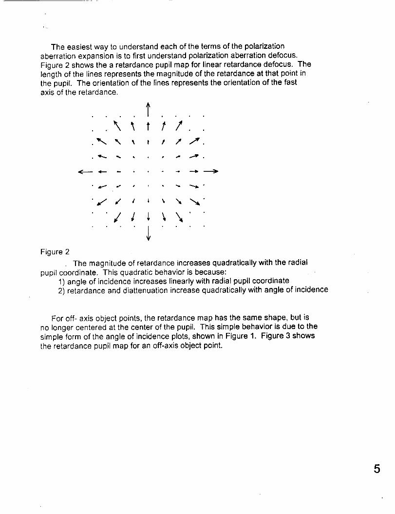
The easiest way to understand each of the terms of the polarizationaberration expansion is to first understand polarization aberration defocus.Figure 2 shows the a retardance pupil map for linear retardance defocus. Thelength of the lines represents the magnitude of the retardance at that point inthe pupil. The orientation of the lines represents the orientation of the fastaxis of the retardance.
t\ ttl
._.. \ _ t f ,," 7.
• _ q_. • , • _ _ .
• j # l _ ,, '_ "_"
Figure 2
The magnitude of retardance increases quadratically with the radialpupil coordinate. This quadratic behavior is because:
1) angle of incidence increases linearly with radial pupil coordinate2) retardance and diattenuation increase quadratically with angle of incidence
For off- axis object points, the retardance map has the same shape, but isno longer centered at the center of the pupil. This simple behavior is due to thesimple form of the angle of incidence plots, shown in Figure 1. Figure 3 showsthe retardance pupil map for an off-axis object point.
5
w
Figure 3
This off-axis retardance map can be decomposed into three components
as follows: Because there is some retardance in the center of the pupil,
we add piston, shown in Figure 4.
Figure 4
6
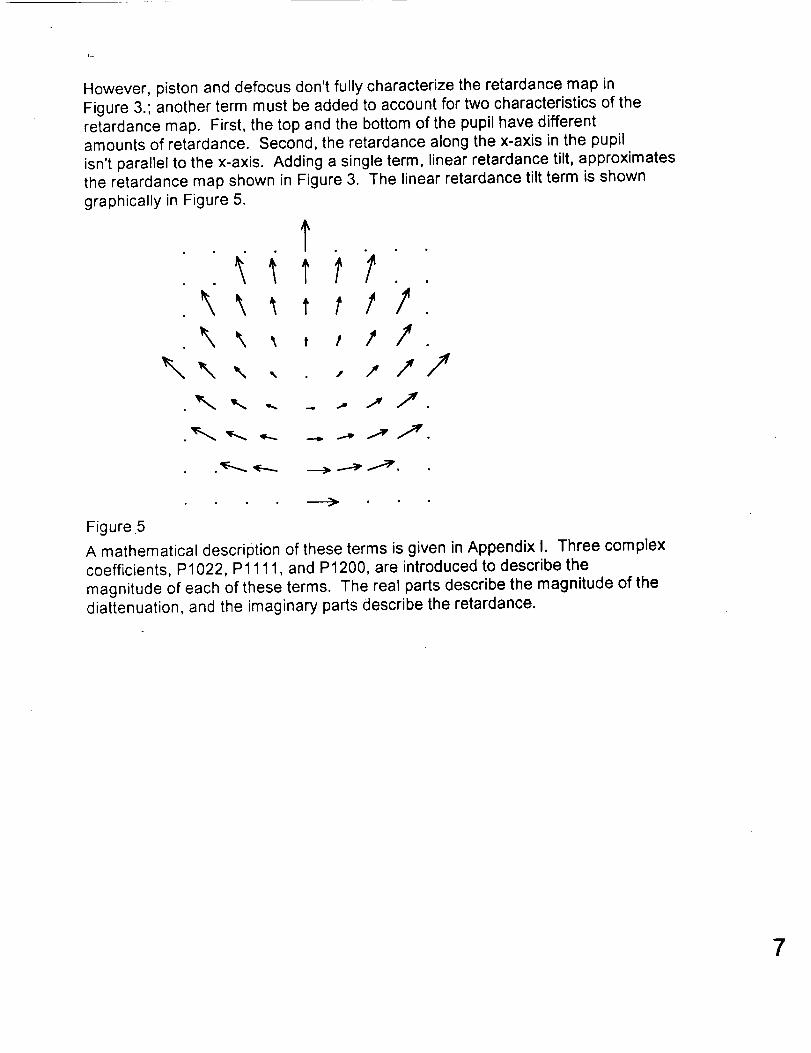
However, piston and defocus don't fully characterize the retardance map in
Figure 3.; another term must be added to account for two characteristics of theretardance map. First, the top and the bottom of the pupil have differentamounts of retardance. Second, the retardance along the x-axis in the pupil
isn't parallel to the x-axis. Adding a single term, linear retardance tilt, approximatesthe retardance map shown in Figure 3. The linear retardance tilt term is shown
graphically in Figure 5.
t
\ \ _ , i I /+\ ",,, ',, ,, , i 1,7
._,_.,,_ .,.... _.,, _ i_i _.
Figure 5
A mathematical description of these terms is given in Appendix I. Three complex
coefficients, P1022, P1111, and P1200, are introduced to describe the
magnitude of each of these terms. The real parts describe the magnitude of the
diattenuation, and the imaginary parts describe the retardance.
7
The polarization aberration coefficients depend on the angles of incidence for the
chief and marginal rays as well as the coatings on the various surfaces. With a tilted
secondary mirror, the angles of incidence on the relevant surfaces are listed in Table 1.
prefilter
primary mirror
secondary mirror
front surface of lens
inner surface of lens
back surface of lens
Angles of Incidence
(with secondary tilted .3 ° )
marginal ray chief ray
0° .16 °
3.6 ° .16 °
4.5 ° .3 °
2.3 ° 2.2 °
9.3 ° 4.7 °
6.5 ° 3.20
For tilted and decentered optical systems, such as the BVM with an articulating
secondary mirror, the meaning of the chief ray and the marginal ray are ambiguous. The
find the chief ray angle of incidence on each surface, we traced rays through the center
of the aperture stop to the center of the field of view and each edge of the field of view.
We called the maximum angle of incidence on that surface the chief ray angle of
incidence. This process was repeated for each of the relevant surfaces. A similar
process was used to find the marginal ray angles of incidence.
Most coating design programs give intensity reflection or transmission coefficients,
but the polarization aberration coefficients are defined in terms of amplitude reflection or
_CKDtNg PAGE BLANK NOT FILMED
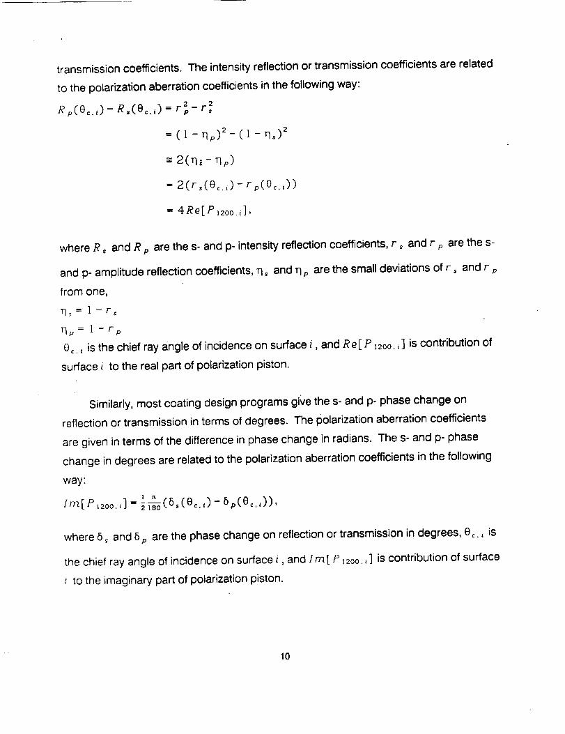
transmission coefficients. The intensity reflection or transmission coefficients are related
to the polarization aberration coefficients in the following way:
Rp(Oc._)- R,(Oc.,) = r 2p- r,2
= (l - qp)_- (l - q,)2
-= 2(q_ - qp)
=2(r,(e_,,)-rp(e_,,))
= 4Re[Pl2oo,,],
where R, and R p are the s- and p- intensity reflection coefficients, r _ and r p
and p- amplitude reflection coefficients, q, and q p are the small deviations of r, and r
from one,
11_ = ] - rs
q_, = I - rp
Oc., is the chief ray angle of incidence on surface i, and Re[ P 12oo. ,] is contribution of
surface L to the real part of polarization piston.
are the s-
Similarly, most coating design programs give the s- and p- phase change on
reflection or transmission in terms of degrees. The polarization aberration coefficients
are given in terms of the difference in phase change in radians. The s- and p- phase
change in degrees are related to the polarization aberration coefficients in the following
way:
] ft
lm[ P ,zoo.,] = 6p(e=.,)),
where 6 _ and 5 p are the phase change on reflection or transmission in degrees, e _. _ is
the chief ray angle of incidence on surface i, and Ira[ P _2oo. i] is contribution of surface
i to the imaginary part of polarization piston.
10
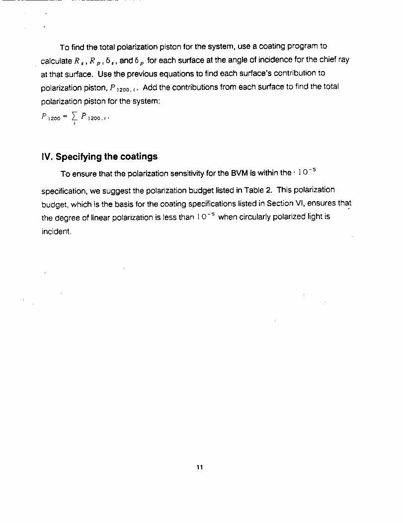
To find the total polarization piston for the system, use a coating program to
calculate R ,, R p, 6,, and 6 p for each surface at the angle of incidence for the chief ray
at that surface. Use the previous equations to find each surface's contribution to
polarization piston, .P _2oo.i. Add the contributions from each surface to find the total
polarization piston for the system:
P12oo = _ P12oo,i'
IV. Specifying the coatings
To ensure that the polarization sensitivity for the BVM is within the. 1 O- 5
specification, we suggest the polarization budget listed in Table 2. This polarization
budget, which is the basis for the coating specifications listed in Section VI, ensures that
the degree of linear polarization is less than ! O-s when circularly polarized light is
0.35" lO -s <ReP 12oo<0.5" lO -s O<Im P izoo<0.005' 10 -s
Re P,2oo=0.08' ]0 -5 ImP Izoo=0
-0.83" lO "s <RePIzoo<-0.5' ]0 -s 0<irn p 1zoo<0.33. ]0 -s,
We also suggest that the mirrors have high reflectivity and the lens surfaces have
high transmission, greater than 98% over the entire range of relevant incident angles and
apertures.
Although we provide simple example coating designs which meet this specification,
we choose not to recommend coating designs with this report because the most
economical way to meet these specifications varies widely from vendor to vendor. Most
vendors have stock coating designs which will meet these specifications, and will not
need to charge for a coating design. To demonstrate the ease of designing coatings
which meet these requirements,
12
Table
Polarization Piston Terms:
Simple coatings
_ RePl2oo IrnP12oo
Pref. Front (LH)4(HL) 4 0.03' lO -s 0.10' lO -s
Pref. Back QWOT MgF 0.01" 10-5 0.0004" 10 -s
Primary HLHLAI -0.005' 10-S -0.04" 10 -5
Secondary HLHLAI -0.02' IO -s -0.12' lO -s
Doub. Front QWOT MgF 0.39' l O -s 0.002" 10 -s
Doub.int. 1 none 0.06" l O-S 0
Doub.lnt. 2 none 0.02" 10-S 0
Doub. Back 4 layer AR -0.79' l o-S 0.30" l O-S
SUM -0.30' 10- s 0.24:10 -s
The coatings should be specified to degrade the surface figure by less than X/10
RMS over the entire clear aperture, to prevent degradation of image quality. Surface
quality should be specified to meet MIL-SPEC 60-40 scratch-dig specifications; this is a
typical surface quality specification for scientific-grade optics. Surface durability should
be specified to meet the MIL-SPEC scotch tape test and eraser test; this is a fairly
stringent requirement, which is justified because this instrument will be used outdoors.
The following three pages describe the polarization errors graphically.
13
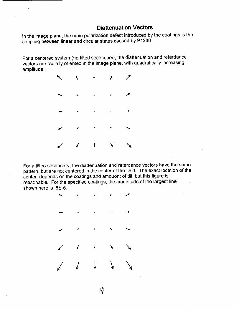
Diattenuation Vectors
In the image plane, the main polarization defect introduced by the coatings is thecoupling between linear and circular states caused by P1200
For a centered system (no tilted secondary), the diattenuation and retardancevectors are radially oriented in the image plane, with quadratically increasing
amplitude..
\ t / 7
For a tilted secondary, the diattenuation and retardance vectors have the samepattern, but are not centered in the center of the field. The exact location of thecenter depends on the coatings and amouont of tilt, but this figure isreasonable. For the specified coatings, the magnitude of the largest lineshown here is .8E-5.
Nasa2
• Effect of other polarization aberrations
In the image plane, the effect of the other polarization aberrations is depo arization.
For a radially symmetric system, this depolarization increases quadraticallyfrom the center of the field of view.
0.5
-0.5
-i
-I -0.5 0 0.5 1
With a tilted secondary, this depolarization increases quadratically
from some other point in the field of view.
The plot shown here is rotated 90 degrees with respect to the diattenuation plots.
1
0.5
-0.5
-I
-i -0.5 0 0.5 1
For the specified coatings, the maximum contour line shown here would beless than 1E-7.
m
16
V. Optical design of the EXVM
While working on the polarization analysis of the NASA-designed instrument, we
noticed that it could be fabricated much more economically if catalog lenses were used
instead of custom lenses. After discussing the possibility with Mona Hagyard, Allen
Gary, and Ed West of NASA, we decided to redesign the optical system to take
advantage of these lenses.
Catalog lenses are lenses which are made for common optical tasks such as
collimating and focussing laser beams. Companies such as Melles-Griot, Spindler &
Hoyer, JML, Newport, Edmund, and CVI have dedicated large amounts of capital to
produce large numbers of commonly-requested focal lengths and diameters. Because
these lenses are made on a regular basis, they are much less expensive than custom
lenses of similar quality.
lens.
Table 4 lists the optical prescription for this system.
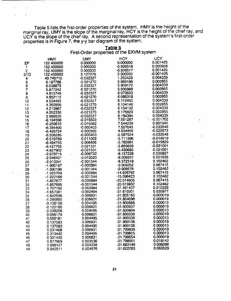
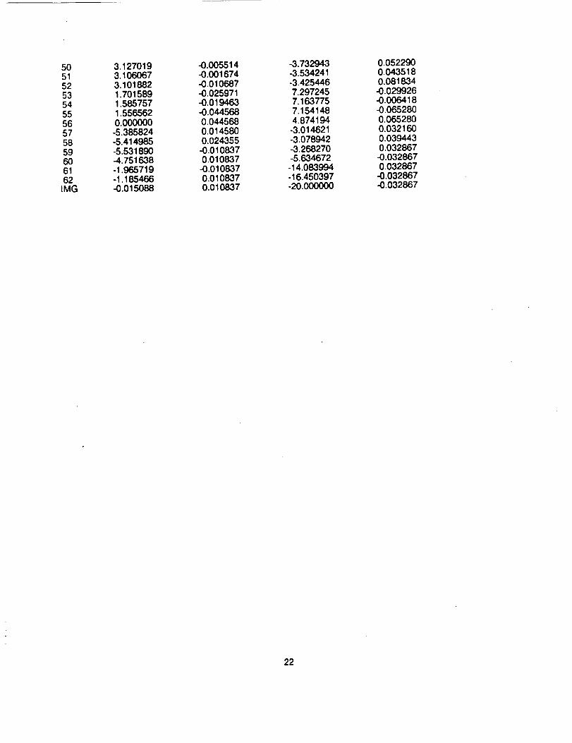
Table 5 lists the first-order properties of the system. HMY is the height of themarginal ray, UMY is the slope of the marginal ray, HCY is the height of the chief ray, andUCY is the slope of the chief ray. A second representation of the system's first-orderproperties is in Figure 7, the y-y bar diagram of the system.
Table 6 lists the surface-by-surface third-order aberrations of the EXVM. SA standsfor spherical aberration, TCO stands for tangential coma, TAS stands for tangentialastigmatism, SAG stands for sa_gital astigmatism, PTB stands for Petzval blur, and DSTstands for distortion. All aberrations are in millimeters.
Iabte_6Third-order aberrations of the EXVM
SA TCO TAS SAG PTB DST1 0.000000 0.000000 0.000000 0.000000 0.000000 0.0000122 0.000000 0.000000 0.000000 0.000000 0.000000 -0.000012
•Figure 8: Wavefront aberrations of the EXVM in the final image plane.
(-FA;_ _. oo aF:__,':._: :,:-F,_
F I ELD _F i GHT0.50 , 0.50
{ . OB',7 °1
i
oo,o , \\
-0.50
/f
4 /
J, .,j/.i
-0,50
0.50
-0.50
0.50
0.00 AEL._,T ]:','E
fiELD HFTGFIT
[ O. 000 °1O. 50
e×','_
-0.50
OPTICAL PATH
7.
DIFFEREHCE (HAVES)
"LG
-0.50
1
I
---- 525.0 1'4M t
I
ORIGINAL PAGE IS
OF POOR QUALITY
Section VI - Coating specification sheets
These optical elements will be used in a solar vector magnetograph, whichmeasures the magnetic fields on the sun's surface by measuring the polarization stateacross the surface of the sun. This particular instrument is designed to makeextraordinarily accurate magnetic field measurements, and therefore, must makeextraordinarily accurate polarization measurements. To make these accuratepolarization measurements, the coatings must be specified to maintain the image'spolarization state very accurately.
The angles of incidence for this system are small, so the polarization associatedwith the surfaces will also tend to be small. The polarization specifications for thesecoatings are meant to ensure that the polarization of the system is small enough to meetits design goals.
The small values for the polarization specifications are justified for several reasons.First, the extreme accuracy of the final instrument would be able to detect any increasefrom these values. Second, since there are several optical elements in the system, thepolarization induced by each element must be small. Finally, although the values for thepolarization specification are small, simple coatings meet the specification.
The example coatings which are included with these specification sheets are meantonly as a guide to vendors. We expect vendors to find stock coatings which are moreappropriate than the example coatings.
27
Prefilter - filter side
diagram of blank
The coating design should meet specifications 1 and 2.
1. Average intensity transmittance - bandpass filter> % over entire diameter, incident angles 0° - .16 °
;k = 525nm
< % outside of nm bandpass, centered on ;_ =525nm
over entire diameter, incident angles 0° - .16 °
2. Polarizationa) Retardance
Retardance is defined as:
A- 8_-8p,
where 8 _ and 8 _ are the phase change on transmission for the s- and p- polarizations
The retardance specification is:0</k <0.00014 °
over entire clear aperture, incident angles 0 ° - .16°
X. = 525nm
b) Intensity DifferenceIntensity difference is defined as:_'Rp-R,,
where R, and R _) are the intensity transmission coefficients for s- and p- polarized light.
The intensity difference specification is:0.0000002 < _ < 0.0000016
over entire clear aperture, incident angles 0° -. 16°
;_ = 525nm
3. Coating thickness variationsThe coating should be deposited with a process which is known to not degrade
transmitted wavefronts by over ;_/5 at 525 nm.
28
4. Surface qualitymust meet MIL-SPEC60-40 scratch-dig specification over entire surface
5. Surface durabilitymust meet MIL-SPECscotch tape and eraser tests over entire surface
The following simple coating meets the polarization specifications. This coating design ismeant only as a guideline for the vendors. The vendors should have stock coatingswhich are more appropriate.
Example coating design:Bandpass filter 1LHLHLHLHHLHLHLHL1.5
where L represents a coating layer of MgF 2 (n = 1.3883) of a thickness equalto one-quarter wave optical path length at X. = 525nm, and where H represents a coatinglayer of ZnS (n = 2.375) of a thickness equal to one-quarter wave optical path length atX. =525nm.
This example coating design gives a retardance value of/k =0.00011 ° and an intensity
difference of _ =0.0000014.
29
Prefilter - backing side
diagram of blank
The coating design should meet specifications 1 and 2.
1. Average intensity transmittance - backing side of filter plate> 97% over entire diameter, incident angles 0° -. 16°X = 525nm
2. Polarization - must be met on each side of prefiltera) Retardance
Retardance is defined as:A-Ss-8 pl
where 8, and 8, are the phase change on transmission for the s- and p- polarizations
The retardance specification is:0 < A < 0.00002 °
over entire clear aperture, incident angles 0° - .16 °
X = 525nm
b) Intensity DifferenceIntensity difference is defined as:
_DE Rp- R,,
where R s and R p are the intensity transmission coefficients for s- and p- polarized light.
The intensity difference specification is:0.0000002 < _ < 0.0000005
over entire clear aperture, incident angles 0° -. 16°
X = 525nm
3. Coating thickness variationsThe coating should be deposited with a process which is known to not degrade
transmitted wavefronts by over X/5 at 525 nm.
4. Surface quality
30
must meet MIL-SPEC 60-40 scratch-dig specification over entire surface
5. Surface durabilitymust meet MIL-SPEC scotch tape and eraser tests over entire surface
A single layer of quarter wave optical thickness at X = 525nm of MgF2 (n = 1.3883)meets the polarization specification. This coating design is meant only as a guideline forthe vendors. The vendors should have stock coatings which are more appropriate. The
example coating design gives retardance of/k = 0.0000004 ° and intensity difference of
= 0.0000004.
31
Primary mirror
diagram of mirror
The coating design must meet specifications 1 and 2:
° Average intensity reflectivity> 98% over entire diameter, incident angles 0 ° - 3.8 °
= 525nm
.
a)Polarization - must be met on each side of prefilterRetardance
Retardance is defined as:
A - 6s- 6_, where
6 s and 6, are the phase change on reflection for the s- and p- polarizations
The retardance specificationis:-0.00008 ° < & < -0.00003 °
5. Surface durabilitymust meet MIL-SPEC scotch tape and eraser tests over entire surface
A simple four-layer reflection-enhancement coating (HLHL) meets thisspecification. L represents a coating layer of MgF2 (n = 1.3883) of a thickness equal toone-quarter wave optical path length at ;_ = 525nm, and H represents a coating layer ofZnS (n = 2.38) of a thickness equal to one-quarter wave optical path length at
= 525nm. This coating design is meant only as a guideline for the vendors. Thevendors can probably design a coating which is more appropriate.
The example coating design gives retardance of _ = -0.00004 ° and an intensity
difference of _ =-0.0000002.
33
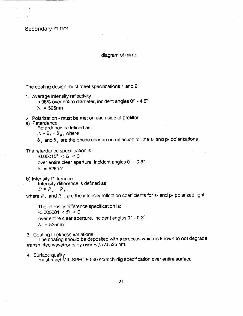
Secondary mirror
diagram of mirror
The coating design must meet specifications 1 and 2:
, Average intensity reflectivity> 98% over entire diameter, incident angles 0° - 4.6 °
X = 525nm
.
a)Polarization - must be met on each side of prefilterRetardance
Retardance is defined as:
A - 6s- 5p, where
6, and 5, are the phase change on reflection for the s- and p- polarizations
The retardance specificationis:-0.00015 ° < & < 0
over entire clear ape_ure, incident angles 0° -0.3 °
X = 525nm
b) Intensity DifferenceIntensity difference is defined as:
_D - R_,- R,,
where R s and R p are the intensity reflection coefficients for s- and p- polarized light.
5. Surface durabilitymust meet MIL-SPEC scotch tape and eraser testsA simple four-layer reflection-enhancement coating (HLHL) meets this
specification. L represents a coating layer of index 1.3883 of a thickness equal to
one-quarter wave optical path length at ;_ = 525nm, and H represents a coating layer of
index 2.38 of a thickness equal to one-quarter wave optical path length at X = 525nm.This coating design is meant only as a guideline for the vendors. The vendors canprobably design a coating which is more appropriate.
The example coating design gives retardance of _ = -0.00014 ° and an intensity
difference of _ =-0.00000068.
35
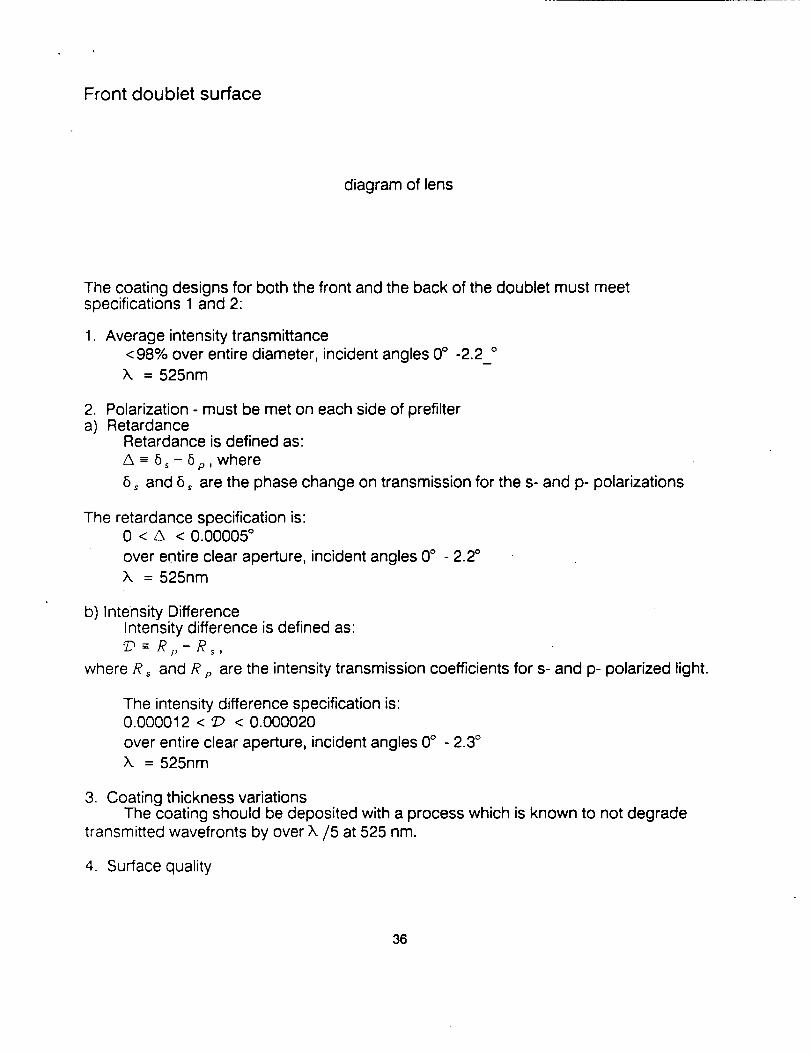
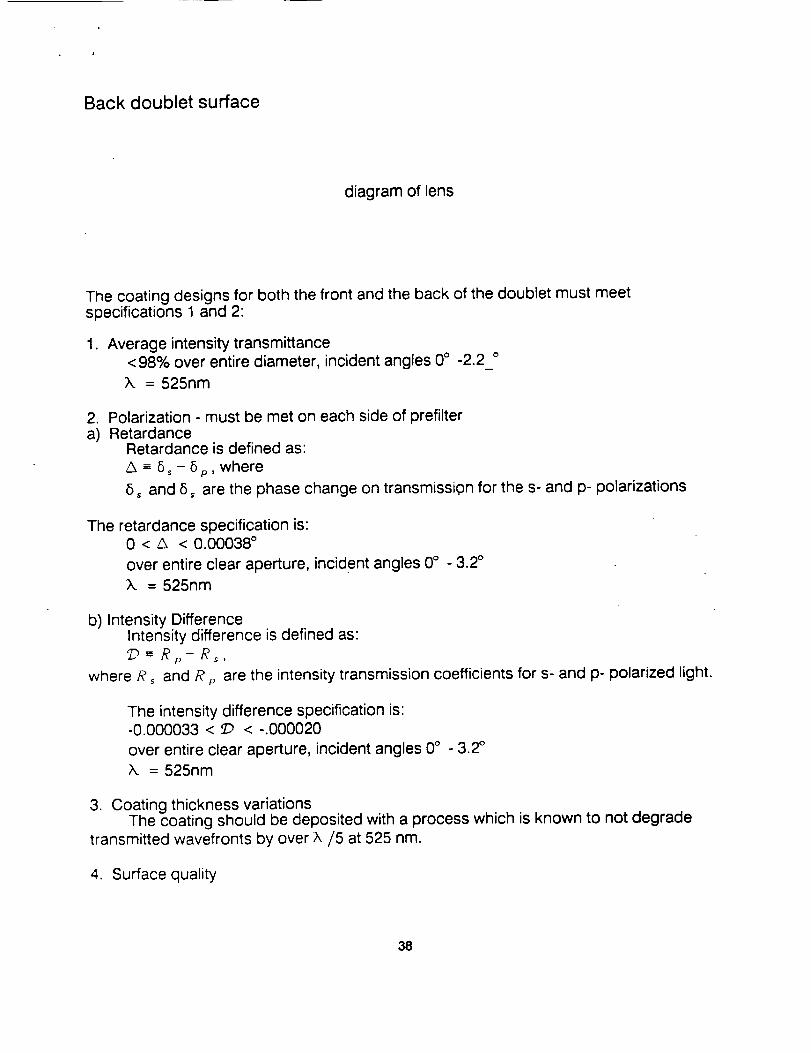
Front doublet surface
diagram of lens
The coating designs for both the front and the back of the doublet must meetspecifications 1 and 2:
1. Average intensity transmittance<98% over entire diameter, incident angles 0° -2.2 °X = 525nm
2. Polarization - must be met on each side of prefiltera) Retardance
Retardance is defined as:
A - 5,- 5p, where
8, and 5, are the phase change on transmission for the s- and p- polarizations
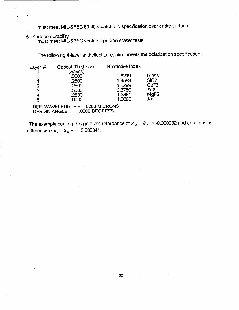
The examp!e coating design gives retardance of R p - R,
difference of 5, - 5 p = = 0.00034 ° .
= -0.000032 and an intensity
39
Appendix I. The paper "Polarization Analysis of the SAMEX SolarMagnetograph" contains both a good summary of polarization aberrationtheory and a good demonstration of polarization aberration analysis.
40
Appendix II. Polarization Aberrations of unresolved point spread functions
This section explicitly provides the mathematics behind the polarization
specification which was presented in the body of the report. First, we present the
reasoning for the derivation of the Mueller matrix averaged over the point spread
function. Next, we derive the average Mueller matrix for rotationally symmetric systems.
Then, we use this Mueller matrix to explore three possible explanations of the ] 0 - s
polarization specification in rotationally symmetric systems. Finally, we explain how the
result from rotationally symmetric systems can be generalized into a result for slightly
decentered systems, such as a vector magnetograph with an actuating secondary
mirror.
In many imaging situations, the point spread function that is formed by the
system's optics is smaller than the resolution of the system's readout. The EXVM is a
good example of this type of system; the pixels on the CCD array are about the same
size as the point spread function.
For this situation, the Stokes vector averaged over the point spread function is
equal to the pupil-averaged Stokes vector. This equality can be understood by
recognizing that the intensity in the pupil of any two orthogonal polarization states is the
same as the intensity of those polarization states in the image. For example, if a 90% of
the intensity in the pupil is y-polarized and 10% is x-polarized, the intensity distribution in
the image plane will also be 90% y-polarized and 10% x-polarized. The polarization state
changes across the pupil and also changes across the point spread function, but the
average Stokes vector will be the same.
This equality can also be derived. The Jones vector in the exit pupil is
41
E= Ey
The Stokes vector in the exit pupil is defined in terms of sums and differences in intensity
measurements,
-5: = I_-I_ :IE:E,.-E_E_
/ 2Re(E' Ey)'
IR--IL k2lm(E_Ey)
where I, Q, U. V are the Stokes vector elements, [ h is the intensity of the light which
would pass through a horizontal polarizer, 1 _ is the intensity of the light which would
pass through a vertical polarizer, l,s. is the intensity of the light which would pass
through a 45 ° polarizer, 1135. is the intensity of the light which would pass through a
135 ° polarizer, ! R is the intensity of light which would pass through a right circular
polarizer, and I L is the intensity which would pass through a left circular polarizer.