Polarization-Corrected Temperatures for 10-, 19-, 37-, and 89-GHzPassive Microwave Frequencies

DANIEL J. CECIL

NASA George C. Marshall Space Flight Center, Huntsville, Alabama

THEMIS CHRONIS

University of Alabama in Huntsville, Huntsville, Alabama

(Manuscript received 19 January 2018, in final form 15 June 2018)

ABSTRACT

Coefficientsarederived for computing thepolarization-corrected temperature (PCT) for 10-, 19-, 37- and89-GHz(and

similar) frequencies, with applicability to satellites in the Global Precipitation Measurement mission constellation and

their predecessors. PCTs for 10- and 19-GHz frequencies have been nonexistent or seldom used in the past; developing

those is themain goal of this study.For 37and89GHz, other formulationsofPCThavealreadybecomewell established.

We consider those frequencies here in order to test whether the large sample sizes that are readily available nowwould

point to different formulations of PCT. The purpose of the PCT is to reduce the effects of surface emissivity differences

in a scene and draw attention to ice scattering signals related to precipitation. In particular, our intention is to develop a

PCT formula that minimizes the differences between land and water surfaces, so that signatures resulting from deep

convection are not easily confusedwithwater surfaces. Thenew formulationsof PCT for 10- and19-GHzmeasurements

hold promise for identifying and investigating intense convection. Four examples are shown from relevant cases. The

PCT for each frequency is effective at drawing attention to themost intense convection, and removing ambiguous signals

that are related to underlying land or water surfaces. For 37 and 89GHz, the older formulations of PCT from the

literature yield generally similar values as ours, with the differences mainly being a few kelvins over oceans. An optimal

formulation of PCT can depend on location and season; results are presented here separated by latitude and month.

1. Introduction

Satellite-borne passive microwave imagers provide in-

formation on the characteristics of Earth’s surface, its

overlying atmosphere, and precipitation. Warm bright-

ness temperatures can result from high emissivity land

surfaces or from emission by liquid cloud or rain hydro-

meteors aloft. Low brightness temperatures can result

from low emissivity surfaces, such as ice and water

bodies, or from scattering by large precipitation ice

particles. Interpretation of the cause of a low bright-

ness temperature can be ambiguous because it could

result from scattering by graupel or hail in a convective

storm, or from a wet or water-covered surface. The

interpretation is especially difficult when an overland

scene includes convective storms, inland water bodies,

and potentially even floodwater or wet soil from recent

precipitation (Fig. 1). This paper aims to enable more

straightforward assessment of the impacts of hydrome-

teors on passive microwave measurements, by mini-

mizing effects due to variability in the underlying surface.

An example of the ambiguity in discriminating storms

from surface conditions is shown in Fig. 1. Strong con-

vective storms are depicted by radar in Fig. 1a, and some

of them produce lower brightness temperatures than the

adjacent land scenes in Figs. 1b–d, especially in the

37-GHz channel (and at higher frequencies, which are not

shownhere). For the lower frequencies,most of the storm-

associated brightness temperatures are no lower than

the precipitation-free brightness temperatures over the

nearby Gulf of Mexico (bottom-right portion of each

panel). Over the eastern part of Texas, there are several

small areas with reduced brightness temperatures that do

not correspond to storms in the radar image. Instead, they

are associated with lakes.

Most current imagers have separate horizontally po-

larized and vertically polarized channels for most fre-

quencies, particularly for frequencies near 10, 19, 37,Corresponding author: Daniel J. Cecil, daniel.j.cecil@nasa.gov

OCTOBER 2018 CEC I L AND CHRON I S 2249

DOI: 10.1175/JAMC-D-18-0022.1

� 2018 American Meteorological Society. For information regarding reuse of this content and general copyright information, consult the AMS CopyrightPolicy (www.ametsoc.org/PUBSReuseLicenses).

Unauthenticated | Downloaded 04/01/22 10:12 PM UTC

and 89GHz. Large polarization differences in the up-

welling brightness temperatures typically result from

water surfaces and surfaces with high soil moisture.

Scattering by large ice hydrometeors typically leads to

much smaller polarization differences. Dry land surfaces

also have smaller polarization differences. A linear com-

bination of horizontally polarized and vertically polarized

brightness temperatures, termed polarization-corrected

temperature (PCT), can remove much of the effect

from varying land surface characteristics (Weinman and

Guetter 1977; Grody 1984; Spencer et al. 1989; Barrett

and Kidd 1990; Todd and Bailey 1995; Kidd 1998;

Toracinta et al. 2002). The PCT is then useful for iden-

tifying scenes with precipitation, with less ambiguity re-

lated to the underlying surface type or surface conditions.

Formulas for PCT have been presented in various forms

in the literature, but here we follow the form

PCTf5 (11Q

f)TB

fV2Q

fTB

fH, (1)

where Q is a coefficient that minimizes the effects of

surface emissivity and TB is the brightness tempera-

ture at frequency f and vertical (V) or horizontal (H)

polarization).

Spatial resolution and sensitivity to typical graupel sizes

both increase with the increasing frequency (decreasing

wavelength) of the radiation. As such, much of the work

involving passive microwave PCT has focused on chan-

nels in the 85–91-GHz range, with some attention also

given to channels near 37GHz. The Spencer et al. (1989)

PCT85 is probably the most widely used today, with the

coefficient Q85 5 0.818 derived from several days of

Special Sensor Microwave Imager (SSM/I; Hollinger

et al. 1990) global observations of cloud-free oceanic

areas. Before settling on this value for Q85, Spencer et al.

(1989) also discussedmodel calculations that imply values

in the range of 0.54–0.61, but those values did not work

well with the observed SSM/I data. The Spencer et al.

(1989) formula was subsequently used in databases of

mesoscale convective systems (Mohr and Zipser 1996)

and more general precipitation features (Nesbitt et al.

2000; Liu et al. 2008), and numerous related studies.

Although Spencer et al. (1989) identified a constantQ85

value in order to apply a uniform standard for global

analysis, others have emphasized that optimal choices of

Q85 can be a function of location, season, and local con-

ditions. Barrett and Kidd (1990) proposedQ85 5 0.64 for

northwestern Europe and the United Kingdom during

summer and autumn. Todd and Bailey (1995) and Kidd

(1998) empirically derivedQ85 values separately for each

scene (each SSM/I overpass of the United Kingdom),

allowing Q85 to vary from day to day. Their Q85 values

generally ranged from about 0.5 to 0.75. Kidd (1998)

showed large daily and intraday variations superimposed

FIG. 1. Example convective outbreak in Texas at 2225 UTC 26 May 2015. (a) Ground-based radar reflectivity

mosaic. GMI (b) 37-, (c) 19-, and (d) 10-GHz vertically polarized brightness temperatures. Contour interval in

(b)–(d) is 25 K, with thick contours every 50K, and theminimumbrightness temperature in the domain is printed in

the panel title.

2250 JOURNAL OF APPL IED METEOROLOGY AND CL IMATOLOGY VOLUME 57

Unauthenticated | Downloaded 04/01/22 10:12 PM UTC

on an apparent annual cycle forQ85, with lowest values in

winter and highest values in summer. Todd and Bailey

(1995) and Kidd (1998) argued that allowing Q85 to vary

with local conditions is important for distinguishing light

rain from rain-free regions.

Before the first SSM/I was launched with its 85-GHz

frequency in 1987, 37-GHz measurements were used

from the Nimbus-6 Electrically Scanning Microwave

Radiometer (ESMR) and Scanning Multichannel Mi-

crowave Radiometer (SMMR). Weinman and Guetter

(1977) developed a linear transformation (they did not

use the term PCT) for use with ESMR. Their Eq. (16)

uses Q37 5 1.2 based on theory and Q37 5 1.5 based

empirically on ESMR observations. Grody (1984) de-

rived Q37 5 1.08 and Q19 5 1.38 for SMMR. Toracinta

et al. (2002) used Q37 5 1.2 for the Tropical Rainfall

Measuring Mission (TRMM; Kummerow et al. 1998)

precipitation feature database (Liu et al. 2008), using

TRMM Microwave Imager (TMI) data. That value

continues to be used for Global Precipitation Measure-

ment (GPM; Hou et al. 2014) mission precipitation fea-

tures. Lee et al. (2002) used Q37 5 1.18, and that value

continues to be used for the popular Naval Research

Laboratory–Monterey tropical cyclone web page. Jiang

et al. (2018) provide a nice discussion of PCT37 and use it

to interpret precipitation types in tropical cyclones.

Precipitation estimation, and more specifically the dis-

crimination between raining and nonraining areas, moti-

vated much of the aforementioned research involving

PCT85. Cecil et al. (2005) and Zipser et al. (2006) em-

phasized the use of PCT37 in studies of intense thun-

derstorms, using TRMM measurements. Cecil (2009)

empirically related TRMM PCT85 and PCT37 to re-

ports of large hail reaching the surface, and Cecil and

Blankenship (2012) applied the PCT37–hail relation-

ship to AdvancedMicrowave Scanning Radiometer for

Earth Observing System (AMSR-E) PCT36 [using the

same Q37 as in Toracinta et al. (2002)] in order to

estimate a global climatology of hailstorm occurrence.

Cecil (2009) also noted that 19-GHz measurements from

TRMM are more effective at giving a high-confidence

indication of large hail, although relatively coarse spatial

resolution and the lack of a well-established PCT19

made it more difficult to use. Mroz et al. (2017) tested an

early version of the PCT19 that is presented here and

found it to bemore effective for identifying hail than any

of the other GMI frequencies.We did not have a version

of PCT10 ready for inclusion in the Mroz et al. study, but

evenwithout applying the PCT, the low-resolution 10-GHz

measurements did show some usefulness in that study.

This paper is motivated by observations of reduced

brightness temperatures in the TRMM and GPM 19-

and 10-GHz channels for some intense thunderstorms,

besides the reduced brightness temperatures that have

already been well documented for the 85–89- and 36–

37-GHz frequencies. Systematic analysis of thunderstorm-

related signatures in the 19- and 10-GHz channels is

difficult without first applying a PCT transformation to

those channels. This paper empirically derives values for

Q10,Q19,Q37, andQ89 from 3 years ofGPMmeasurements

and considers their spatial and seasonal variability. The

main goal is to derive and evaluate useful coefficients for

PCT10 and PCT19, since those have rarely been used in the

past. The values for Q37 and Q89 from the literature have

proven effective over the years. We reexamine them here

because it has become convenient to apply our methods to

vastly larger sample sizes than were used in the previous

studies. Our optimal coefficients (producing the smallest

contrast between land and water surfaces, and thus less

ambiguity related to surface type) for PCT37 and PCT89 are

slightly different from those that have already been widely

used. Our analysis shows that a broad range of coefficient

values can be defensible for these frequencies, when applied

to global studies. As such, there may be little practical

benefit for many users in switching from the previous

Q37 andQ89 values to our marginally more effective values.

The values derived for Q10 and Q19 do show promise for

enabling improved analysis of vigorous, deep convection.

2. Data and methods

GPM Microwave Imager (GMI) version V05A

brightness temperatures (GESDISC 2016) from 1 April

2014 to 31March 2017 are used for development of PCT

coefficients in this study. Every other GPM orbit (odd-

numbered orbits from 503 to 17 553) and every 10th scan

position (of the 221 positions per GMI scan) are used, in

order to speed up the required processing. This amounts

to using 5% of the available data during a 3-yr period,

while still sampling a broad variety of conditions.

TheGMI level 2 (‘‘GPROF’’) files (Iguchi andMeneghini

2016) are further used to identify precipitation-free

pixels, and to classify each pixel as land (GPROF sur-

face types 3–5, corresponding to ‘‘maximum vegetation,’’

‘‘high vegetation,’’ and ‘‘moderate vegetation’’) or ocean

(GPROF surface type 1). The ‘‘ocean’’ classification can

include large water bodies, for example, the Great

Lakes. Sea ice, arid regions, surface snow cover, rivers,

coasts, and precipitation scenes are excluded.

Each orbit is divided into 58 latitude bins. Statistics

are derived separately for each of these bins that has at

least 10 land and 10 water pixels without precipitation.

Latitude bins without enough land and water pixels in a

given orbit are ignored, because a comparison between

land and water pixels is required for building the empir-

ical relationships. For a given latitude bin in a givenGPM

OCTOBER 2018 CEC I L AND CHRON I S 2251

Unauthenticated | Downloaded 04/01/22 10:12 PM UTC

orbit, candidate PCT values using a given Q are com-

puted for each pixel. The differences betweenPCT values

are then computed for every possible pairing of land and

water pixels within that latitude bin. If there are 10 land

and 10water pixels, for example, therewould be 100 pairs

with land–water PCT differences. Since the GMI swath is

about 900km wide and the satellite only takes a few

minutes to traverse 58, most of the land–water differences

are computed within a few hundred kilometers and a few

minutes of each other. Ideally, a perfect choice of Qwould yield PCT differences near zero for all possible

land–water pairings, and a poor choice of Q would yield

large PCT differences. That ideal scenario is not realistic,

because inhomogeneities in a scene besides surface type

would give nonzero differences. A histogram of PCT

differences is computed from the land–water pairings and

added to histograms computed from other orbits. This

process is repeated for candidate PCT values computed

with Q ranging from 0.3 to 1.79 in increments of 0.01.

Each GMI frequency under consideration is treated

separately, at its native resolution.

The PCT difference histograms are computedwith bin

size of 2K. They are accumulated separately for each

58 latitude bin, for each month of the year, and for each

Q value. Even though we considered only 5% of the

available GMI data, before further restricting the data

by surface type and precipitation, most latitudes (from

558S to 608N) and months contain tens of millions of

land–water pairings for the resulting histograms. The

sample size (Table 1) is relatively small at far the

southern latitudes because there is so little land there,

and is large at the far northern latitudes because of both

orbital geometry and the mix of land and ocean surfaces.

The seasonal variation in sample size is extreme at

far northern latitudes (2 million land–water pairings in

January, 357 million pairings in August) because the

surface snow and ice cover are eliminated.

The resulting histograms of land–water PCT differ-

ences are analyzed in section 3 to determine which Qvalues most consistently yield small PCT differences. A

small difference in PCT between land and water pixel

pairs indicates that the surface type is not strongly influ-

encing the PCT, and that we can use PCT to investigate

precipitation hydrometeor signatures instead. Section 3a

accumulates the histograms into probability density func-

tions across all latitudes and months for a global analysis,

and section 3b examines variability by latitude andmonth.

PCT coefficients based on the results from section 3

are applied to selected cases in section 4. Those cases

were observed individually by theGMI, TMI, AMSR-E,

and SSM/I sensors (Table 2). The GPM Intercalibration

(X-CAL)Working Group dataset (Berg et al. 2016; GES

DISC 2016, 2017a,b,c) is used for these, since it applies an

intercalibration among sensors, making their calibrations

consistent with GMI. The X-CAL brightness tempera-

tures are referred to as GPM level 1C version 05A, with

TABLE 1. Sample size (in millions) of land–water pairings for each 58 latitude bin (bottom latitude of the bin is listed in the first column)

and each month.

Lat (8) Jan Feb Mar Apr May Jun Jul Aug Sep Oct Nov Dec

55 2 4 17 136 273 293 338 357 308 200 38 6

50 6 8 26 153 209 225 241 255 221 164 53 11

45 12 21 65 133 159 173 180 193 165 143 85 29

40 43 47 91 112 118 119 127 133 120 115 96 62

35 81 75 112 122 128 129 125 128 116 117 109 96

30 72 68 86 87 89 84 82 86 80 79 87 87

25 78 70 82 75 69 61 52 53 60 60 74 84

20 75 71 86 76 73 65 40 34 38 45 60 73

15 58 59 73 68 58 45 36 37 38 32 45 55

10 108 111 120 101 92 85 72 77 86 82 89 100

5 104 112 123 95 96 94 91 95 91 89 98 100

0 103 97 101 86 98 97 98 108 108 102 100 100

25 86 80 80 72 92 91 95 103 100 95 91 88

210 85 80 84 83 103 102 110 121 119 111 103 89

215 89 83 90 94 120 113 121 132 130 124 108 94

220 81 78 85 86 104 95 99 108 114 104 99 86

225 77 75 79 79 95 84 87 92 93 82 82 77

230 76 72 74 78 95 83 85 90 91 81 83 76

235 90 88 83 86 97 88 89 93 97 88 95 91

240 50 48 47 45 46 42 41 41 44 41 48 52

245 28 27 26 26 25 22 20 20 22 23 26 28

250 17 16 16 16 17 13 12 12 16 15 16 18

255 6 5 6 6 6 5 3 3 5 5 5 6

2252 JOURNAL OF APPL IED METEOROLOGY AND CL IMATOLOGY VOLUME 57

Unauthenticated | Downloaded 04/01/22 10:12 PM UTC

other satellites included as GPM constellation members.

GPM level 1B version 05A 85-GHz data (GES DISC

2017d) are also used for the TMI case, because level 1C

unnecessarily sets values below 50K asmissing.AMSR-E

level 2A version 3 files (Ashcroft and Wentz 2013) from

the National Snow and Ice Data Center (NSIDC) are

also used for 89GHz for the same reason.

3. Results: Optimizing PCT coefficients

a. Global analysis

First, we consider statistics from the land–water PCT

differences accumulated over all months and all regions.

Since a motivation for using the PCT is to eliminate the

land–water differences as much as possible, Fig. 2 shows

what percentage of land–water pairs have PCT differences

below 2K (thick lines) and below 10K (thin lines) as a

function of the choice ofQ value. For convenience, we will

refer to the value yielding land–water PCT differences less

than 2K the most often as the ‘‘best’’ performing Q in a

given analysis. These are not the Q values we ultimately

recommend using. Defining the best Q based on how

rarely it produces large (.10K) differences would lead to

Q values 0.03–0.04 higher. Our ultimate recommendations

will consider both those definitions and the regional and

seasonal variability to be addressed in section 3b.

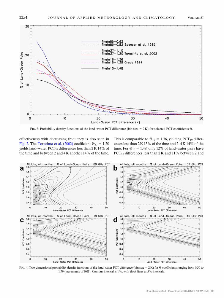
Figure 3 shows probability density functions of land–

water PCT differences for the Q values that yield PCT

differences of less than 2K most often and for some

other Q values from the literature. For Q89 5 0.63, 24%

of land–water pairings have PCT differences less than

2K, another 21% have differences between 2 and 4K,

and 16% have differences of 4–6K. Using Q89 5 0.82

based on Spencer et al. (1989) reduces those percentages

to 18%, 17%, and 16%, respectively. The best-

performing Q37 (1.10) in this global analysis yields

land–water differences in PCT37 that are slightly larger

than the differences in PCT89 based on using the Spencer

et al. Q85. In other words, a suboptimal choice of Q89 can

outperform an optimal choice of Q37. Moving to still

lower-frequency channels, the best-performingQ19 (1.36)

and Q10 (1.48) are progressively less effective at mini-

mizing the land–water PCT differences. This decreasing

TABLE 2. Footprint sizes (effective fields of view; km) for the frequencies and instruments used in this study.

Sensor

GMI (Hou

et al. 2014)

TMI (Kummerow

et al. 1998)

AMSR-E

(JAXA 2006)

SSM/I (Hollinger

et al. 1990)

Frequency (GHz) 10.65 18.7 36.5 89.0 10.7 19.35 37.0 85.5 10.65 18.7 36.5 89.0 19.35 37.0 85.5

Along track 32 18 15 7 63 30 16 7 51 27 14 6 69 37 15

Cross track 19 11 9 4 37 18 9 5 29 16 8 4 43 28 13

FIG. 2. Percentage of land–water PCT differences less than 2K (thick lines) and less than 10K (thin lines), as a function of Q value.

OCTOBER 2018 CEC I L AND CHRON I S 2253

Unauthenticated | Downloaded 04/01/22 10:12 PM UTC

effectiveness with decreasing frequency is also seen in

Fig. 2. The Toracinta et al. (2002) coefficient Q37 5 1.20

yields land–water PCT37 differences less than 2K 14% of

the time and between 2 and 4K another 14% of the time.

This is comparable to Q19 5 1.36, yielding PCT19 differ-

ences less than 2K 15% of the time and 2–4K 14% of the

time. For Q10 5 1.48, only 12% of land–water pairs have

PCT10 differences less than 2K and 11% between 2 and

FIG. 3. Probability density functions of the land–water PCT difference (bin size 5 2K) for selected PCT coefficients Q.

FIG. 4. Two-dimensional probability density functions of the land–water PCT difference (bin size5 2K) forQ coefficients ranging from 0.30 to

1.79 (increments of 0.01). Contour interval is 1%, with thick lines at 5% intervals.

2254 JOURNAL OF APPL IED METEOROLOGY AND CL IMATOLOGY VOLUME 57

Unauthenticated | Downloaded 04/01/22 10:12 PM UTC

4K. For this ‘‘best’’ choice ofQ10 from the global analysis,

about half the land–water pairs have PCT10 differences

greater than 10K. Any choice of Q10 will have many sit-

uations where it is not very effective at removing the

land–water contrast.

The probability density functions in Fig. 3 isolated the

Q values that gave the sharpest peaks in the 0–2-K PCT

difference bins. Figure 4 instead depicts the performance

for all Q values, in the form of two-dimensional proba-

bility density functions. The sideways V shapes for these

two-dimensional probability density functions indicate

that for each frequency, there is a preferred range of Qvalues where the land–water PCT differences tend to be

small. Moving away from that preferred range, Q values

that are too high or too low give larger land–water PCT

differences. Minimizing those land–water differences is

crucial for seamlessly interpreting the precipitation

characteristics across a coastline, or in a scene including

small water bodies. A narrow range of Q values gives

acceptably small land–water PCT differences for the low-

frequency channels, but a broad range ofQ89 values gives

small PCT89 differences.

b. Variability by latitude and month

Figures analogous to Figs. 2–4 were generated sepa-

rately for each 58 latitude bin and for each month. Lower

Q values generally have better performance (i.e., less

variation in PCT) in the deep tropics than at higher

latitudes. At mid- and high latitudes, higher Q values

performbetter during thewarm season and lowerQ values

perform better during the cold season. The Q values that

yield the highest percentage of land–water pairs with

PCT differences less than 2K are compiled as functions

of latitude and month in Table 3 (89GHz), Table 4

(37GHz), Table 5 (19GHz), and Table 6 (10GHz).

Just as a range of Q values works better for higher-

frequency channels than any Q value does for lower-

frequency channels in Figs. 2–4, a range ofQ values also

works well in the tropics, compared to higher latitudes.

As an example, the effectiveness of each Q value at re-

ducing the land–water contrast below 2K (thick lines)

and below 10K (thin lines) as in Fig. 2 is reproduced

separately for 08–58N in July (Fig. 5) and for 358–408N in

July (Fig. 6). The best-performing Q values are lower in

the tropics than in the midlatitudes (consistent with

Tables 3–6). The PCT is so much more effective at re-

ducing the land–water contrast in the deep tropics, thus

there is little need to find the precise Q value that gives

the best scores there. One could choose whichever

Q value is most acceptable for the midlatitudes, and that

Q would also work well in the tropics.

4. Discussion and examples

Consideration of Figs. 2–4, analogous figures that are

segregated by latitude and month, and Tables 3–6 leads

TABLE 3. The 89-GHz PCT coefficient Q89 for each latitude and month that gives the most land–water pixel pairs with PCT

differences , 2 K.

Lat (8) Jan Feb Mar Apr May Jun Jul Aug Sep Oct Nov Dec

55 0.54 0.57 0.60 0.63 0.64 0.72 0.74 0.69 0.61 0.55 0.58 0.62

50 0.52 0.53 0.56 0.60 0.64 0.80 0.74 0.72 0.63 0.55 0.56 0.57

45 0.55 0.58 0.60 0.66 0.69 0.79 0.77 0.67 0.64 0.58 0.57 0.58

40 0.51 0.56 0.58 0.59 0.64 0.72 0.66 0.63 0.61 0.58 0.55 0.53

35 0.48 0.55 0.55 0.63 0.65 0.75 0.67 0.66 0.62 0.57 0.51 0.48

30 0.46 0.51 0.58 0.65 0.69 0.78 0.70 0.65 0.66 0.56 0.49 0.41

25 0.44 0.56 0.65 0.73 0.82 0.70 0.68 0.66 0.61 0.59 0.55 0.46

20 0.51 0.57 0.70 0.83 0.81 0.74 0.64 0.51 0.54 0.58 0.56 0.51

15 0.59 0.64 0.68 0.77 0.73 0.68 0.64 0.59 0.57 0.54 0.58 0.58

10 0.62 0.68 0.73 0.85 0.87 0.85 0.74 0.64 0.66 0.69 0.60 0.61

5 0.65 0.71 0.73 0.69 0.66 0.63 0.57 0.53 0.58 0.61 0.62 0.61

0 0.58 0.63 0.57 0.52 0.52 0.56 0.59 0.57 0.59 0.60 0.60 0.60

25 0.59 0.62 0.56 0.52 0.56 0.61 0.61 0.64 0.64 0.63 0.61 0.61

210 0.52 0.55 0.49 0.51 0.57 0.65 0.66 0.68 0.70 0.67 0.57 0.53

215 0.53 0.50 0.50 0.52 0.59 0.65 0.65 0.68 0.69 0.64 0.58 0.51

220 0.68 0.62 0.59 0.63 0.61 0.64 0.62 0.64 0.72 0.75 0.72 0.68

225 0.81 0.77 0.70 0.67 0.66 0.61 0.60 0.63 0.73 0.81 0.78 0.82

230 0.84 0.85 0.77 0.72 0.63 0.59 0.60 0.63 0.70 0.81 0.77 0.84

235 0.84 0.80 0.74 0.68 0.64 0.57 0.60 0.61 0.65 0.75 0.73 0.79

240 0.78 0.76 0.72 0.63 0.62 0.58 0.58 0.58 0.62 0.72 0.72 0.77

245 0.71 0.66 0.62 0.58 0.55 0.49 0.52 0.54 0.55 0.66 0.62 0.67

250 0.74 0.67 0.67 0.61 0.56 0.51 0.53 0.56 0.56 0.62 0.69 0.70

255 0.81 0.69 0.70 0.59 0.57 0.57 0.56 0.58 0.61 0.59 0.76 0.71

OCTOBER 2018 CEC I L AND CHRON I S 2255

Unauthenticated | Downloaded 04/01/22 10:12 PM UTC

to the conclusion that while no single Q value gives an

ideal PCT formulation applicable to all places and

seasons, a range of Q values can generally give credible

results. Some readers may wish to use PCT formulations

that are most appropriate for particular regions or sea-

sons, and Tables 3–6 are suitable for selecting those

Q values. Others, including ourselves, will want to

apply a single Q value for each frequency globally, all

TABLE 5. As in Table 3, but for the 19-GHz PCT coefficient Q19.

Lat (8) Jan Feb Mar Apr May Jun Jul Aug Sep Oct Nov Dec

55 1.29 1.30 1.32 1.33 1.34 1.43 1.42 1.40 1.34 1.28 1.29 1.29

50 1.28 1.29 1.34 1.37 1.39 1.49 1.44 1.42 1.38 1.33 1.32 1.29

45 1.28 1.35 1.40 1.43 1.44 1.48 1.49 1.44 1.41 1.37 1.35 1.31

40 1.29 1.34 1.34 1.36 1.40 1.45 1.43 1.40 1.38 1.35 1.32 1.29

35 1.28 1.34 1.36 1.40 1.43 1.48 1.48 1.43 1.40 1.37 1.31 1.28

30 1.23 1.28 1.36 1.41 1.42 1.47 1.42 1.38 1.38 1.33 1.26 1.25

25 1.24 1.29 1.33 1.39 1.39 1.38 1.37 1.35 1.34 1.31 1.30 1.26

20 1.29 1.37 1.37 1.42 1.39 1.38 1.35 1.29 1.31 1.31 1.30 1.31

15 1.32 1.38 1.42 1.41 1.38 1.37 1.38 1.33 1.33 1.30 1.31 1.31

10 1.62 1.69 1.74 1.79 1.57 1.52 1.48 1.42 1.41 1.39 1.39 1.39

5 1.37 1.43 1.41 1.38 1.37 1.36 1.33 1.31 1.32 1.32 1.33 1.35

0 1.32 1.34 1.32 1.30 1.29 1.31 1.30 1.31 1.32 1.31 1.31 1.31

25 1.33 1.35 1.32 1.30 1.32 1.33 1.33 1.34 1.35 1.34 1.34 1.32

210 1.32 1.33 1.31 1.30 1.33 1.35 1.36 1.39 1.39 1.37 1.34 1.32

215 1.33 1.33 1.31 1.30 1.33 1.35 1.37 1.40 1.41 1.39 1.35 1.32

220 1.42 1.39 1.38 1.37 1.35 1.41 1.43 1.46 1.59 1.63 1.58 1.46

225 1.53 1.48 1.48 1.44 1.46 1.49 1.51 1.56 1.59 1.70 1.68 1.59

230 1.49 1.47 1.44 1.42 1.40 1.40 1.43 1.42 1.47 1.59 1.48 1.51

235 1.57 1.47 1.49 1.46 1.42 1.39 1.41 1.43 1.44 1.51 1.49 1.58

240 1.48 1.44 1.44 1.39 1.40 1.34 1.35 1.38 1.38 1.45 1.47 1.49

245 1.67 1.66 1.59 1.38 1.49 1.39 1.39 1.45 1.41 1.49 1.56 1.68

250 1.79 1.75 1.72 1.55 1.53 1.49 1.51 1.53 1.53 1.61 1.73 1.75

255 1.66 1.59 1.57 1.47 1.43 1.43 1.44 1.45 1.43 1.48 1.55 1.59

TABLE 4. As in Table 3, but for the 37-GHz PCT coefficient Q37.

Lat (8) Jan Feb Mar Apr May Jun Jul Aug Sep Oct Nov Dec

55 0.97 0.98 1.01 1.03 1.03 1.11 1.12 1.10 1.05 0.98 0.98 1.00

50 0.96 0.97 0.99 1.03 1.07 1.17 1.13 1.13 1.08 1.02 1.00 0.98

45 0.98 1.01 1.03 1.07 1.11 1.17 1.18 1.14 1.11 1.04 1.02 1.00

40 0.97 1.01 1.01 1.03 1.09 1.15 1.12 1.12 1.09 1.05 1.01 0.99

35 0.95 1.01 1.04 1.08 1.12 1.18 1.17 1.14 1.12 1.07 1.01 0.98

30 0.96 0.99 1.07 1.11 1.14 1.20 1.17 1.14 1.13 1.08 1.01 0.98

25 0.97 1.06 1.07 1.14 1.13 1.12 1.12 1.10 1.10 1.06 1.05 0.99

20 1.02 1.09 1.13 1.20 1.14 1.14 1.11 1.05 1.06 1.06 1.05 1.04

15 1.08 1.12 1.15 1.19 1.16 1.14 1.17 1.10 1.09 1.06 1.07 1.07

10 1.25 1.27 1.35 1.42 1.32 1.28 1.24 1.17 1.16 1.16 1.17 1.23

5 1.14 1.19 1.18 1.15 1.13 1.12 1.08 1.07 1.07 1.08 1.08 1.11

0 1.07 1.10 1.08 1.05 1.04 1.06 1.06 1.06 1.07 1.07 1.06 1.06

25 1.08 1.10 1.07 1.05 1.07 1.09 1.09 1.10 1.11 1.09 1.10 1.07

210 1.08 1.09 1.06 1.06 1.09 1.12 1.12 1.16 1.15 1.14 1.09 1.08

215 1.08 1.08 1.06 1.05 1.09 1.11 1.12 1.14 1.15 1.13 1.10 1.07

220 1.16 1.15 1.12 1.12 1.11 1.14 1.13 1.17 1.23 1.30 1.26 1.18

225 1.25 1.24 1.21 1.17 1.17 1.17 1.16 1.21 1.25 1.35 1.30 1.30

230 1.27 1.23 1.21 1.19 1.16 1.13 1.12 1.16 1.21 1.28 1.23 1.30

235 1.31 1.22 1.23 1.19 1.14 1.08 1.09 1.13 1.15 1.20 1.21 1.27

240 1.22 1.18 1.18 1.11 1.10 1.04 1.04 1.06 1.07 1.15 1.17 1.21

245 1.20 1.19 1.14 1.08 1.08 1.01 1.01 1.04 1.04 1.12 1.14 1.18

250 1.30 1.22 1.21 1.09 1.09 1.04 1.05 1.08 1.08 1.14 1.22 1.22

255 1.27 1.17 1.17 1.08 1.05 1.04 1.04 1.05 1.07 1.08 1.17 1.17

2256 JOURNAL OF APPL IED METEOROLOGY AND CL IMATOLOGY VOLUME 57

Unauthenticated | Downloaded 04/01/22 10:12 PM UTC

through the year. The most straightforward choice

would be to take the Q values highlighted in section 3a,

but instead we recommend some slight modifications to

account for varying performance in different regions

and seasons. Our recommendations (Table 7) also round

the Q values to the nearest 0.05, since Figs. 2–4 and the

analysis by latitude and by month suggest that precision

to the nearest 0.01 is not warranted.

TABLE 6. As in Table 3, but for the 10-GHz PCT coefficient Q10.

Lat (8) Jan Feb Mar Apr May Jun Jul Aug Sep Oct Nov Dec

55 1.47 1.50 1.53 1.53 1.53 1.61 1.58 1.55 1.49 1.45 1.47 1.48

50 1.47 1.50 1.55 1.54 1.54 1.65 1.58 1.55 1.52 1.49 1.48 1.47

45 1.44 1.49 1.73 1.79 1.58 1.63 1.63 1.57 1.55 1.53 1.49 1.47

40 1.48 1.54 1.56 1.57 1.58 1.62 1.58 1.53 1.52 1.51 1.49 1.48

35 1.45 1.53 1.57 1.60 1.61 1.63 1.62 1.51 1.50 1.52 1.46 1.46

30 1.36 1.40 1.50 1.55 1.55 1.57 1.52 1.48 1.48 1.44 1.38 1.37

25 1.36 1.41 1.46 1.49 1.50 1.50 1.47 1.45 1.44 1.42 1.38 1.37

20 1.40 1.47 1.47 1.51 1.50 1.47 1.45 1.40 1.42 1.42 1.42 1.43

15 1.42 1.47 1.50 1.49 1.48 1.47 1.46 1.43 1.43 1.41 1.41 1.42

10 1.79 1.79 1.79 1.78 1.68 1.64 1.58 1.53 1.51 1.48 1.48 1.79

5 1.46 1.50 1.49 1.46 1.46 1.45 1.43 1.42 1.43 1.42 1.43 1.43

0 1.42 1.44 1.43 1.42 1.41 1.42 1.40 1.41 1.42 1.42 1.42 1.41

25 1.43 1.45 1.42 1.41 1.42 1.43 1.43 1.44 1.45 1.44 1.45 1.43

210 1.43 1.44 1.42 1.40 1.43 1.45 1.45 1.49 1.49 1.47 1.44 1.43

215 1.44 1.44 1.42 1.41 1.43 1.45 1.50 1.51 1.52 1.49 1.46 1.43

220 1.54 1.50 1.49 1.47 1.45 1.57 1.59 1.66 1.75 1.79 1.79 1.61

225 1.64 1.57 1.61 1.55 1.67 1.71 1.73 1.78 1.79 1.79 1.79 1.79

230 1.59 1.56 1.54 1.53 1.51 1.51 1.58 1.56 1.60 1.73 1.61 1.62

235 1.69 1.58 1.62 1.58 1.58 1.55 1.57 1.59 1.61 1.71 1.66 1.72

240 1.62 1.57 1.55 1.52 1.55 1.50 1.52 1.59 1.54 1.59 1.61 1.61

245 1.56 1.53 1.53 1.79 1.79 1.76 1.77 1.79 1.79 1.79 1.53 1.53

250 1.62 1.56 1.59 1.79 1.79 1.79 1.79 1.79 1.79 1.79 1.58 1.59

255 1.79 1.79 1.79 1.79 1.79 1.77 1.79 1.78 1.76 1.79 1.79 1.79

FIG. 5. Percentage of land–water PCT differences less than 2K (thick lines) and less than 10K (thin lines), as a function ofQ value, for the

08–58N latitude bin during July.

OCTOBER 2018 CEC I L AND CHRON I S 2257

Unauthenticated | Downloaded 04/01/22 10:12 PM UTC

The result that a high degree of precision is not

warranted in selecting Q values also suggests that the

same coefficients should be appropriate for use with

other passive microwave sensors, despite differences in

footprint sizes or radiometer frequencies. Small varia-

tions in the frequencies used by different radiometers

can lead to brightness temperature differences of a few

kelvins in rain-free regions (or several kelvins in rain,

but raining pixels are omitted from the computation of

PCT coefficients) (Yang et al. 2014). If the entire anal-

ysis were repeated using an 85.5-GHz (e.g., SSM/I

or TMI) or 91.7-GHz (e.g., SSM/I/Sounder) frequency

instead of the GMI’s 89.0-GHz frequency, there might

be small changes in the details in section 3, but

likely no significant change in the choice ofQ. Likewise,

differences in the sensors’ footprint sizes should have

little effect, especially since the analysis is done using

precipitation-free pixels.

For passivemicrowave channels in the range 85–92GHz

(including SSM/I, TMI, GMI, and AMSR), we recom-

mend Q89 5 0.70. This tends more toward the higher

values that workwell in themidlatitudewarm seasons than

the lower values that work best in the tropics, since per-

formance of PCT89 in the tropics is less sensitive to the

precise choice of Q89. For similar reasons, we recommend

Q37 5 1.15 for the 36–37-GHz channels on SSM/I, TMI,

GMI, and AMSR.

Many publications have usedQ855 0.818 andQ375 1.2

for PCT based on Spencer et al. (1989) and Toracinta

et al. (2002), particularly for studies involving TRMM

FIG. 6. As in Fig. 5, but for the 358–408N latitude bin.

TABLE 7. The PCT coefficients Q from this study and from the literature.

Source 85–89GHz 36–37GHz 19GHz 10GHz

This study 0.70 (GMI) 1.15 (GMI) 1.40 (GMI) 1.50 (GMI)

Spencer et al. (1989) 0.818 (SSM/I)

0.54–0.61 (model)

Toracinta et al. (2002) 1.20 (TMI)

Weinman and Guetter (1977) 1.50 (ESMR)

1.20 (model)

Grody (1984) 1.08 (SMMR) 1.38 (SMMR)

Barrett and Kidd (1990) 0.64 (SSM/I)

Todd and Bailey (1995); Kidd (1998) 0.5–0.75 (SSM/I)

Lee et al. (2002) 1.18

2258 JOURNAL OF APPL IED METEOROLOGY AND CL IMATOLOGY VOLUME 57

Unauthenticated | Downloaded 04/01/22 10:12 PM UTC

and GPM precipitation feature databases (Nesbitt et al.

2000; Liu et al. 2008). Figures 7 and 8 compare PCT

values computed using our recommended Q values to

those computed using the Spencer et al. (1989) and

Toracinta et al. (2002) values. The differences aremostly

small, which was expected because the Spencer et al. and

Toracinta et al. versions have both proven effective over

the years. Figures 2 and 4 show that these small changes

do tend to slightly reduce the land–water contrasts when

using our new versions of PCT89 and PCT37. Since the

PCT formula in Eq. (1) can be rearranged to include a

term with Qmultiplying the polarization difference, our

lower choices of Q almost always lead to slightly lower

PCT values. The choice of Q has least effect where po-

larization differences are small (e.g., most land areas)

and greatest effect where polarization differences are

large (e.g., water surfaces beneath optically thin air

masses). For PCT89, the differences are less than 1K

over most land areas and 1–4K over most ocean loca-

tions. Exceptions over land are deserts and areas of snow

or ice cover, where PCT89 tends to be 1–3K lower using

our choice of Q89. Over oceans, the largest differences

(4–8K) coincide with dry air masses, particularly at mid-

and high latitudes. For PCT37, the differences over land

are again less than 1K except for deserts and snowpacks,

where the differences are 1–2K. Over oceans, the dif-

ferences are only 2–4K, with the higher values co-

inciding with drier air masses. For both frequencies, the

differences are only a few tenths of a kelvin for pixels

with substantial precipitation signatures.

FIG. 7. Difference between PCT89 computed using Q85 5 0.818 (Spencer et al. 1989)

minus that using Q89 5 0.70 (from this study). Three days of GPM orbits (26–28 May 2015)

are mapped.

FIG. 8. Difference between PCT37 computed usingQ375 1.20 (Toracinta et al. 2002) minus

that using Q37 5 1.15 (from this study). Three days of GPM orbits (26–28 May 2015) are

mapped.

OCTOBER 2018 CEC I L AND CHRON I S 2259

Unauthenticated | Downloaded 04/01/22 10:12 PM UTC

For 19-GHz channels (including SSM/I, TMI, GMI,

and AMSR), we recommend Q19 5 1.40. This is essen-

tially the same (after rounding) as the 1.38 value used by

Grody (1984), with which we were not familiar until

preparing this manuscript. For channels near 10GHz

(TMI, GMI, and AMSR), we recommend Q10 5 1.50.

As with the higher-frequency channels, these rec-

ommendations for the lower-frequency channels are

compromises that are intended to work best in both the

tropics and during midlatitude warm seasons. For the

lower-frequency channels, the ability to eliminate dif-

ferences between land and water-covered scenes is

substantially reduced compared to the higher-frequency

channels.

We briefly consider cases with intense convective

storms that were observed by GMI, TMI, AMSR-E, and

FIG. 9. GMI case from west of FortWorth on 26May 2015: (left) vertically polarized brightness temperature and

(right) PCT. Contour interval is 25K, with thick contours every 50K. The minimum brightness temperature (or

PCT) of the domain is printed.

2260 JOURNAL OF APPL IED METEOROLOGY AND CL IMATOLOGY VOLUME 57

Unauthenticated | Downloaded 04/01/22 10:12 PM UTC

SSM/I, in order to demonstrate the utility of these new

PCT formulations. These cases were previously identi-

fied by Cecil (2015) as having some of the most extreme

37- or 89-GHz scattering signatures for those satellites.

For each example in Figs. 9–12, the left panels show

vertically polarized brightness temperatures and the

right panels show PCT (using our recommended co-

efficients, as in Table 7).

The storms around Texas shown in Fig. 1 are revisited

in Fig. 9, a case observed by GMI on 26 May 2015. At

89GHz (Figs. 9a,b), the effect of the PCT is not espe-

cially noticeable for this case, other than bringing the

Gulf of Mexico temperatures closer to those over land.

For the 37-, 19-, and 10-GHz frequencies, the PCT

eliminates the sharp gradient at the coast and also

eliminates the signatures associated with lakes that were

FIG. 10. As in Fig. 9, but for a TMI case from northern Argentina on 30 Dec 1997. (a),(b) The TB85V and PCT85

were rederived with X-CAL offsets applied to level 1B files, because the level 1C X-CAL files have values below

50K set as missing.

OCTOBER 2018 CEC I L AND CHRON I S 2261

Unauthenticated | Downloaded 04/01/22 10:12 PM UTC

mentioned in Fig. 1. The individual figure panels identify

the minimum brightness temperature (or PCT) for each

panel. Most of these minima are associated with the

strongest storm, west of Fort Worth, Texas. The mini-

mum TB10V (Fig. 9g) is a precipitation-free Gulf of

Mexico scene, but PCT10 (Fig. 9h) is minimized over the

storm, as desired.

A case over northern Argentina observed by TMI is

shown in Fig. 10. The left panels have low brightness

temperatures from numerous intense thunderstorms,

along with low surface emissivity features such as the

ParanaRiver, IberaWetlands, and theMar Chiquita salt

lake. The PCT in the right panels only highlight the

strong storms. Zipser et al. (2006) highlighted this case

FIG. 11. As in Fig. 9, but for AMSR-E case of Typhoon Bolaven east of the Philippines on 18 Nov 2005.

(a),(b) The TB89V and PCT89 were taken from AMSR-E level 2A brightness temperatures distributed by NSIDC,

because the level 1CX-CAL files have values below 50K set as missing. Comparison of nearby pixels slightly above

50K suggests the calibrations are consistent within 1.0 K.

2262 JOURNAL OF APPL IED METEOROLOGY AND CL IMATOLOGY VOLUME 57

Unauthenticated | Downloaded 04/01/22 10:12 PM UTC

and mentioned its lowest PCT37 as 69K. Its minimum

PCT37 is higher (74K) in Fig. 10d because of two cali-

brations that were applied to TMI since that paper. The

update from TRMM version 7 to version 8 (now known

as GPM version 5, because TRMM is treated as part of

the GPM constellation) increased TB37V and TB37H by

2.8 and 2.5K, respectively, for the coldest pixel in this

case. The recalibration for consistency with GMI

(known as the GPM X-CAL level 1C brightness tem-

peratures) increases TB37V by 0.69K and decreases

TB37H by 1.56K for the low end of TB37 values, such as

this. The increased TB37V 2 TB37H polarization

difference adds to the PCT37. The change from using

Toracinta et al.’s (2002) Q37 coefficient [also used by

Zipser et al. (2006)] to ours only amounts to a 0.3-K

difference between the two formulations.

Typhoon Bolaven (2005) is shown in Fig. 11, as ob-

served near the Philippines (east of Luzon) by AMSR-E

on 18 November 2005. The use of PCT again eliminates

most of the land–water contrast (with the Philippines

on the far left of each panel). But the PCT also removes

much of the signal from rain in the lower-frequency

channels. Emission by liquid rain is seen as warm

brightness temperatures over ocean in the left panels,

but only the scattering by large ice particles is high-

lighted by the PCT in the right panels.

The SSM/I has coarser resolution than GMI, TMI, and

AMSR-E, and lacks a 10-GHz channel, but the PCT

highlights intense convection in SSM/I’s 19-, 37-, and

85-GHz frequencies. The ‘‘Boundary Waters Derecho’’

(Price and Murphy 2002) case (Fig. 12) featured an in-

tense storm in northern Minnesota. The PCT is again

effective at removing the signal associated with the lakes

in this region and drawing attention to the storm.

The cases shown in Figs. 9–12 were selected because

they were known to have extremely low PCT37 values,

so they were good candidates for having substantial ice

scattering signatures in the 19- and 10-GHz channels.

Indeed, the GMI and TMI cases had PCT19 reduced

from near 300K in the surrounding areas to 159 and

FIG. 12. As in Fig. 9, but for an SSM/I case from Minnesota on 4 Jul 1999.

OCTOBER 2018 CEC I L AND CHRON I S 2263

Unauthenticated | Downloaded 04/01/22 10:12 PM UTC

149K, respectively, at the convective cores. Those two

cases also had noticeable scattering signatures in PCT10

(241 and 265K, respectively), despite the longer wave-

length and coarser resolution for this frequency (Table 2).

The AMSR-E case (Typhoon Bolaven; Fig. 11) had

weaker signatures in the low-frequency channels (235-K

PCT19; 278-K PCT10) than the GMI and TMI cases, but

it also had a weaker signature at 37GHz (113K). It had

the lowest TBV89 (41K) and PCT89 (41K) values of all

these cases, which may result from having an extraordi-

narily deep vertical layer of large graupel. The SSM/I case

from Minnesota had PCT19 reduced to 230K, despite

SSM/I’s coarse resolution. Another SSM/I case from the

same region (28 June 1998) had PCT19 scattered to 217K

(not shown).

5. Conclusions

Coefficients have been derived for computing PCT for

10-, 19-, 37- and 89-GHz (and similar) frequencies from

GMI and related radiometers. While coefficient values

can be optimized for particular regions and seasons us-

ing Tables 3–6, we recommend the values listed in

Table 7 for global applications. These result in the fol-

lowing formulas:

PCT105 2.5TB

10V2 1.5TB

10H, (2)

PCT195 2.4TB

19V2 1.4TB

19H, (3)

PCT375 2.15TB

37V2 1.15TB

37H, and (4)

PCT895 1.7TB

89V2 0.7TB

89H. (5)

These values were tested using four cases with intense

convection observed separately by the GMI, TMI,

AMSR-E, and SSM/I sensors. The new PCT formulations

eliminated much of the contrast between land and water

surfaces in all four cases and for all four frequencies. The

intense convection is easily recognized with PCT de-

pressions in each case, without having surface-related

characteristics contributing other ambiguous PCT

depressions.

Other formulations of PCT89 and PCT37 have become

well established. Differences between our PCT89 and

that from Spencer et al. (1989) and between our PCT37

and that fromToracinta et al. (2002) were examined and

tend to be small, especially for measurements involving

ice scattering related to precipitation. Otherwise, our

PCT89 and PCT37 tend to be a few kelvins lower than the

previous formulations over the oceans. The largest dif-

ferences are over relatively dry oceanic air masses.

Differences over land are usually less than 1K, except

for deserts and snow- or ice-covered regions.

The key new developments from this paper are the

coefficients for computing PCT19 and PCT10. We see

these as tools for further investigating intense thunder-

storms, using GPM and other satellites with related

sensors. Indeed, Mroz et al. (2017) obtained higher skill

scores for hail detection using a preliminary version of

our PCT19 than the scores obtained using higher fre-

quencies or individual polarizations. Here, PCT19 and

PCT10 essentially mask the signals that come from in-

land water bodies or from coasts. They also have little

sensitivity to most precipitation, but help draw attention

to the most intense convection, capable of producing

large amounts of hail and/or graupel that scatter the

upwelling radiation in these frequencies.

Acknowledgments. This research is supported by

NASA’s Precipitation Measurement Mission Science

Team (NNH15ZDA001N-PMM). GPM data provided

by the National Aeronautics and Space Administration

(NASA) and the Japan Aerospace Exploration Agency

(JAXA) through the Precipitation Processing System

website (http://pps.gsfc.nasa.gov/).

REFERENCES

Ashcroft, P., and F. J. Wentz, 2013. AMSR-E/Aqua L2A Global

Swath Spatially-Resampled Brightness Temperatures, Ver-

sion 3. Distributed Active Archive Center, NASA National

Snow and Ice Data Center, accessed 18 June 2013, https://

dx.doi.org/10.5067/AMSR-E/AE_L2A.003.

Barrett, E. C., and C. Kidd, 1990: Rainfall monitoring by the SSM/I

in middle latitudes. Fifth Conf. on Satellite Meteorology and

Oceanography, London, United Kingdom, Amer. Meteor.

Soc., 210–214.

Berg, W., and Coauthors, 2016: Intercalibration of the GPM mi-

crowave radiometer constellation. J. Atmos. Oceanic Technol.,

33, 2639–2654, https://doi.org/10.1175/JTECH-D-16-0100.1.

Cecil, D. J., 2009: Passive microwave brightness temperatures

as proxies for hailstorms. J. Appl. Meteor. Climatol., 48,

1281–1286, https://doi.org/10.1175/2009JAMC2125.1.

——, 2015: Extremely low passive microwave brightness temper-

atures due to thunderstorms. 20th Conf. on Satellite Meteo-

rology and Oceanography, Phoenix, AZ, Amer. Meteor. Soc.,

J13.1A, https://ams.confex.com/ams/95Annual/webprogram/

Paper266429.html.

——, and C. B. Blankenship, 2012: Toward a global climatology of se-

vere hailstorms as estimated by satellite passivemicrowave imagers.

J. Climate, 25, 687–703, https://doi.org/10.1175/JCLI-D-11-00130.1.

——, S. J. Goodman, D. J. Boccippio, E. J. Zipser, and S. W.

Nesbitt, 2005: Three years of TRMM precipitation features.

Part I: Radar, radiometric, and lightning characteristics.Mon.

Wea. Rev., 133, 543–566, https://doi.org/10.1175/MWR-2876.1.

GES DISC, 2016: GPM_1BGMI: GPM GMI brightness tempera-

tures L1B 1.5 hours 13 kmV05. Goddard Earth Sciences Data

and Information Services Center, accessed 24 May 2017,

https://doi.org/10.5067/GPM/GMI/GPM/1B/05.

——, 2017a: GPM_1CTRMMTMI: GPM TMI on TRMM com-

mon calibrated brightness temperatures L1C 1.5 hours

2264 JOURNAL OF APPL IED METEOROLOGY AND CL IMATOLOGY VOLUME 57

Unauthenticated | Downloaded 04/01/22 10:12 PM UTC

13 kmV05. Goddard Earth Sciences Data and Information

Services Center, accessed 28 December 2017, https://doi.org/

10.5067/GPM/TMI/TRMM/1C/05.

——, 2017b: GPM_1CAQUAAMSRE: GPM AMSR-E on

AQUA common calibrated brightness temperatures L1C

1.5 hours 10.5 kmV05. Goddard Earth Sciences Data and

Information Services Center, accessed 28 December 2017,

https://doi.org/10.5067/GPM/AMSRE/AQUA/1C/05.

——, 2017c: GPM SSMI on F14 common calibrated brightness

temperatures L1C 1.5 hours 13 kmV05. Goddard Earth

Sciences Data and Information Services Center, accessed 28

December 2017, https://doi.org/10.5067/GPM/SSMI/F14/1C/05.

——, 2017d: GPM_1BTMI: GPM TMI on TRMM brightness

temperatures L1B 1.5 hours 13 kmV05. Goddard Earth

Sciences Data and Information Services Center, accessed 28

December 2017, https://doi.org/10.5067/GPM/TMI/TRMM/1B/05.

Grody, N. C., 1984: Precipitation monitoring over land from sat-

ellites by microwave radiometry. Proc. Int. Geosciences and Re-

mote Sensing Symp., Strasbourg, France, ESA SP-215, 417–423.

Hollinger, J. P., J. L. Pierce, andG.A. Poe, 1990: SSM/I instrument

evaluation. IEEE Trans. Geosci. Remote Sens., 28, 781–790,

https://doi.org/10.1109/36.58964.

Hou, A. Y., and Coauthors, 2014: The Global Precipitation Mea-

surement Mission. Bull. Amer. Meteor. Soc., 95, 701–722,

https://doi.org/10.1175/BAMS-D-13-00164.1.

Iguchi, T., and R. Meneghini, 2016: GPM_2AGPROFGPMGMI:

GPM GMI (GPROF) radiometer precipitation profiling L2A

1.5 hours 13 kmV05. Goddard Earth Sciences Data and In-

formation Services Center, accessed 24 May 2017, https://

doi.org/10.5067/GPM/GMI/GPM/GPROF/2A/05.

JAXA, 2006: AMSR-E data users handbook. 4th ed. Japan Aero-

space Exploration Agency, 115 pp., http://www.eorc.jaxa.jp/en/

hatoyama/amsr-e/amsr-e_handbook_e.pdf.

Jiang, H., J.P. Zagrodnik, C. Tao, and E.J. Zipser, 2018: Classifying

precipitation types in tropical cyclones using the NRL 37GHz

color product. J. Geophys. Res. Atmos., 123, 5509–5524, https://

doi.org/10.1029/2018JD028324.

Kidd, C., 1998: On rainfall retrieval using polarization-corrected

temperatures. Int. J. Remote Sens., 19, 981–996, https://doi.org/

10.1080/014311698215829.

Kummerow, C.,W. Barnes, T. Kozu, J. Shiue, and J. Simpson, 1998:

The Tropical Rainfall Measuring Mission (TRMM) sensor

package. J. Atmos. Oceanic Technol., 15, 809–817, https://doi.org/

10.1175/1520-0426(1998)015,0809:TTRMMT.2.0.CO;2.

Lee, T. F., F. J. Turk, J. Hawkins, and K. Richardson, 2002: In-

terpretation of TRMMTMI images of tropical cyclones.Earth

Interact., 6, https://doi.org/10.1175/1087-3562(2002)006,0001:

IOTTIO.2.0.CO;2.

Liu, C., E. J. Zipser, D. J. Cecil, S. W. Nesbitt, and S. Sherwood,

2008: A cloud and precipitation feature database from nine

years of TRMM observations. J. Appl. Meteor. Climatol., 47,

2712–2728, https://doi.org/10.1175/2008JAMC1890.1.

Mohr, K. I., and E. J. Zipser, 1996: Defining mesoscale convective

systems by their 85-GHz ice-scattering signatures.Bull. Amer.

Meteor. Soc., 77, 1179–1189, https://doi.org/10.1175/1520-

0477(1996)077,1179:DMCSBT.2.0.CO;2.

Mroz, K., A. Battaglia, T. J. Lang, D. J. Cecil, S. Tanelli, and

F. Tridon, 2017: Hail detection algorithm for the GPM core

satellite sensors. J. Appl. Meteor. Climatol., 56, 1939–1957,

https://doi.org/10.1175/JAMC-D-16-0368.1.

Nesbitt, S. W., E. J. Zipser, and D. J. Cecil, 2000: A census of pre-

cipitation features in the tropics using TRMM: Radar, ice scatter-

ing, and lightning observations. J. Climate, 13, 4087–4106, https://

doi.org/10.1175/1520-0442(2000)013,4087:ACOPFI.2.0.CO;2.

Price, C.G., and B.P. Murphy, 2002: Lightning activity during the

1999 Superior derecho. Geophys. Res. Lett., 29, 2142, https://

doi.org/10.1029/2002GL015488.

Spencer, R. W., H. M. Goodman, and R. E. Hood, 1989: Pre-

cipitation retrieval over land and ocean with the SSM/I:

Identification and characteristics of the scattering signal.

J. Atmos. Oceanic Technol., 6, 254–273, https://doi.org/

10.1175/1520-0426(1989)006,0254:PROLAO.2.0.CO;2.

Todd, M. C., and J. O. Bailey, 1995: Estimates of rainfall over

the United Kingdom and surrounding seas from the SSM/I

using the polarization-corrected temperature algorithm.

J. Appl. Meteor., 34, 1254–1265, https://doi.org/10.1175/1520-

0450(1995)034,1254:EOROTU.2.0.CO;2.

Toracinta, E. R., D. J. Cecil, E. J. Zipser, and S. W. Nesbitt, 2002:

Radar, passive microwave, and lightning characteristics of

precipitating systems in the tropics. Mon. Wea. Rev., 130,

802–824, https://doi.org/10.1175/1520-0493(2002)130,0802:

RPMALC.2.0.CO;2.

Weinman, J. A., and P. J. Guetter, 1977: Determination of rainfall

distributions from microwave radiation measured by Nimbus

6 ESMR. J. Appl.Meteor., 16, 437–442, https://doi.org/10.1175/

1520-0450(1977)016,0437:DORDFM.2.0.CO;2.

Yang, S., J. Hawkins, andK. Richardson, 2014: The improvedNRL

tropical cyclone monitoring system with a unified microwave

brightness temperature calibration scheme. Remote Sens., 6,

4563–4581, https://doi.org/10.3390/rs6054563.

Zipser, E. J., C. Liu, D. J. Cecil, S.W. Nesbitt, andD. P. Yorty, 2006:

Where are the most intense thunderstorms on Earth? Bull.

Amer. Meteor. Soc., 87, 1057–1071, https://doi.org/10.1175/

BAMS-87-8-1057.

OCTOBER 2018 CEC I L AND CHRON I S 2265

Unauthenticated | Downloaded 04/01/22 10:12 PM UTC