Vol. 4, No. 12/December 1987/J. Opt. Soc. Am. A 2205
Polarization properties of speckle patterns scattered fromrough conductors
Yeshayahu Fainman, Joseph Shamir, David Peri, and Andrei Brunfeld
Department of Electrical Engineering, Technion- Israel Institute of Technology, Haifa 32000, Israel
Received July 25, 1986; accepted August 12, 1987
The scattered field amplitude and its polarization and statistics are represented as functions of illuminating field,and surface statistics. The random contribution to the field is separated from its deterministic part and expandedinto several terms of decreasing orders of magnitude for detailed study. Various terms can be emphasized by propersystem design to extract specific information about surface parameters. Preliminary experiments confirm novelpredictions related to the correlations of polarized speckle patterns.
1. INTRODUCTION
Coherent light scattered from a rough surface carries muchinformation about the surface, and it is interesting to findeasily applicable mathematical relations that connect thescattered-light characteristics with the surface parameters.
The complicated nature of the scattering of electromag-netic radiation from randomly rough surfaces prompted var-ious approaches toward its mathematical analysis.1-' 6
These approaches differ in the mathematical tools utilized,the degree of approximations, and their limits of validity.Usually the results are also limited to special groups of ex-perimental situations, such as illumination at normal inci-dence and measurement along the plane of incidence only.The research reported here is an additional step toward theunderstanding of the complex nature of the field and inten-sity distributions due to scattering by a rough surface.
Using a conventional approach, the scattered field distri-bution may be calculated from a given current distributionover the surface of the scatterer.17'1 8 We assume that thephysical-optics approximation' is valid and calculate thescattered field resulting from the illumination of an idealrough conductor by a coherent plane wave. The compactnotation and approach of the operator algebra'9-2 ' intro-duced at this point provide a simplified derivation leading toquite general applicability of the final expressions. Manypolarization phenomena may be deduced, without mathe-matical calculations, just by separating the deterministiccontribution from the random one. Although many of thesephenomena are known1"8 in general, the derivation here issimple, and the final mathematical expressions lend them-selves to further study.
The properties of the speckle pattern are related in Sec-tions 3 and 4 to scattering surface statistics. A series expan-sion of the surface correlation function leads to the predic-tion of novel interesting phenomena that were qualitativelydemonstrated by preliminary experiments.
2. SCATTERED FIELD POLARIZATION
The scattering process treated in this paper is shown sche-matically in Fig. 1. A monochromatic, coherent plane wave
with its wave vector ki having a magnitude k = 27r/X illumi-nates a planar rough surface. The transversal coordinates,xl' and x2', are defined in the average plane of the object,while the third coordinate, X3', is perpendicular to it. Theobservation point P is referred to a coordinate system inwhich X3 coincides with X3', while x1 and x2 are parallel to xl'and x2', respectively.
It can be shown22-26 that the field scattered by the roughsurface may be expressed in the form
u(x) = jk(I + I VV A(X), (1)
where the dyadic notation was adopted, with 1 denoting theunit dyad. A is the vector potential of the current sourcegenerated by the incident illumination through the induc-tion theorem. The exact calculation, however, is too compli-cated, and we shall show that fair results can be obtained byusing a number of approximations applicable to variousphysical situations. In what follows we assume that thesurface is a perfect conductor and that the physical-opticsapproximation can be applied [i.e., (X/a)2
<< 1, with X thewavelength of the illuminating light and a the minimal radi-us of curvature of the local surface roughness].
We denote the transverse coordinates over the object sur-face and observation planes, respectively, by
p = X1'11 + X2'SX2,
r = xlpl + X2X2
(2)
(3)
and replace X3' by h(p), the height of the roughness distribu-tion above the average surface plane. From simple geomet-rical considerations, the transversal components of the sur-face unit vector are equal to the derivatives of h(p). Fur-thermore, with the above assumptions, these componentsare very small compared to unity, and we may state theapproximate relation:
(4)
In Appendix A we give the definition of the basic operatorsconstituting the operator algebral9 -21 and derive the Green's
2206 J. Opt. Soc. Am. A/Vol. 4, No. 12/December 1987
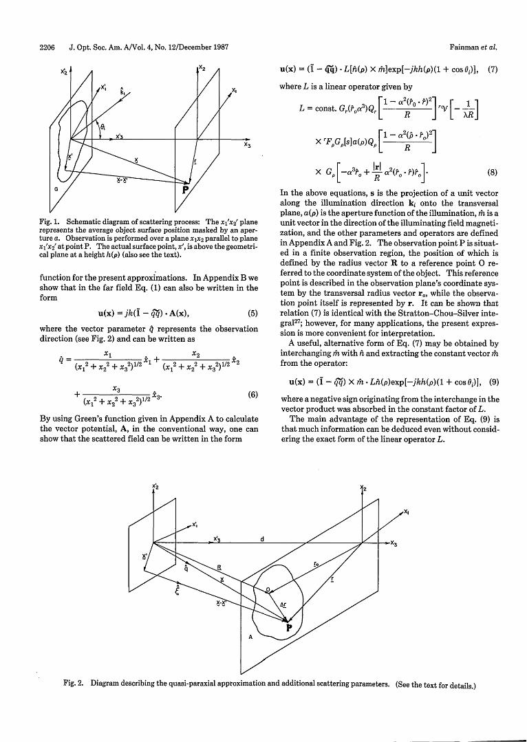
Fig. 1. Schematic diagram of scattering process: The xl'x2' planerepresents the average object surface position masked by an aper-ture a. Observation is performed over a plane x1x2 parallel to planeXl'X2' at point P. The actual surface point, x', is above the geometri-cal plane at a height h(p) (also see the text).
function for the present approximations. In Appendix B weshow that in the far field Eq. (1) can also be written in theform
u(x) = jk(I - qq) * A(x), (5)
where the vector parameter q represents the observationdirection (see Fig. 2) and can be written as
q (x2 + X22 + X32 )l/ 2 l (xI2 + x22 + x 2)1/2 X2
+ (X12 + X3(XI2 + X2
2 + X32)'1/
2X
(6)
By using Green's function given in Appendix A to calculatethe vector potential, A, in the conventional way, one canshow that the scattered field can be written in the form
u(x) = (I - Q) -L[h(p) X rh]exp[-jkh(p)(1 + cos 0)], (7)
where L is a linear operator given by
L = const. Gr(Poca3)Q [1 -a(P* rc, [_ ]
x rF G [sla(p)Qp [ --ao- (P °]
(8)
In the above equations, s is the projection of a unit vectoralong the illumination direction ki onto the transversalplane, a(p) is the aperture function of the illumination, mh is aunit vector in the direction of the illuminating field magneti-zation, and the other parameters and operators are definedin Appendix A and Fig. 2. The observation point P is situat-ed in a finite observation region, the position of which isdefined by the radius vector R to a reference point 0 re-ferred to the coordinate system of the object. This referencepoint is described in the observation plane's coordinate sys-tem by the transversal radius vector r0 , while the observa-tion point itself is represented by r. It can be shown thatrelation (7) is identical with the Stratton-Chou-Silver inte-gral27; however, for many applications, the present expres-sion is more convenient for interpretation.
A useful, alternative form of Eq. (7) may be obtained byinterchanging mh with h and extracting the constant vector thfrom the operator:
u(x) = (I-qq) X m - Lh(p)exp[-jkh(p)(l + cos 0)], (9)
where a negative sign originating from the interchange in thevector product was absorbed in the constant factor of L.
The main advantage of the representation of Eq. (9) isthat much information can be deduced even without consid-ering the exact form of the linear operator L.
x,I
Fig. 2. Diagram describing the quasi-paraxial approximation and additional scattering parameters. (See the text for details.)
Fainman et al.
X G , [_.3p� + Irl a 2(p, . p)p,)R I
Vol. 4, No. 12/December 1987/J. Opt. Soc. Am. A 2207
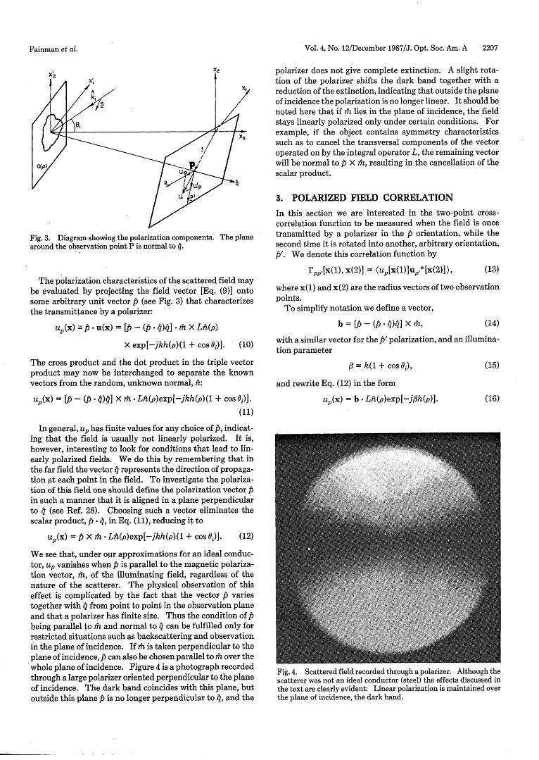
Fig. 3. Diagram showing the polarization components. The planearound the observation point P is normal to 0.
The polarization characteristics of the scattered field maybe evaluated by projecting the field vector [Eq. (9)] ontosome arbitrary unit vector D (see Fig. 3) that characterizesthe transmittance by a polarizer:
up(x) - iu(x) = Lb- (P -04)q - m X Lh(p)
X exp[-jkh(p)(1 + cos 0i)]. (10)
The cross product and the dot product in the triple vectorproduct may now be interchanged to separate the knownvectors from the random, unknown normal, h:
up(x) = [b - ( - OM] X mh * Lh(p)exp[-jkh(p)(1 + cos 0i)].
(11)
In general, up has finite values for any choice of P, indicat-ing that the field is usually not linearly polarized. It is,however, interesting to look for conditions that lead to lin-early polarized fields. We do this by remembering that inthe far field the vector q represents the direction of propaga-tion at each point in the field. To investigate the polariza-tion of this field one should define the polarization vector Din such a manner that it is aligned in a plane perpendicularto 0 (see Ref. 28). Choosing such a vector eliminates thescalar product, Db - , in Eq. (11), reducing it to
up(x) = D X 7h -Lh(p)exp[-jkh(p)(1 + cos 0)]. (12)
We see that, under our approximations for an ideal conduc-tor, up vanishes when P is parallel to the magnetic polariza-tion vector, rh, of the illuminating field, regardless of thenature of the scatterer. The physical observation of thiseffect is complicated by the fact that the vector D variestogether with from point to point in the observation planeand that a polarizer has finite size. Thus the condition of kbeing parallel to m and normal to q can be fulfilled only forrestricted situations such as backscattering and observationin the plane of incidence. If mh is taken perpendicular to theplane of incidence, i can also be chosen parallel to mh over thewhole plane of incidence. Figure 4 is a photograph recordedthrough a large polarizer oriented perpendicular to the planeof incidence. The dark band coincides with this plane, butoutside this plane i is no longer perpendicular to q, and the
polarizer does not give complete extinction. A slight rota-tion of the polarizer shifts the dark band together with areduction of the extinction, indicating that outside the planeof incidence the polarization is no longer linear. It should benoted here that if m lies in the plane of incidence, the fieldstays linearly polarized only under certain conditions. Forexample, if the object contains symmetry characteristicssuch as to cancel the transversal components of the vectoroperated on by the integral operator L, the remaining vectorwill be normal to P X mh, resulting in the cancellation of thescalar product.
3. POLARIZED FIELD CORRELATION
In this section we are interested in the two-point cross-correlation function to be measured when the field is oncetransmitted by a polarizer in the b orientation, while thesecond time it is rotated into another, arbitrary orientation,,b'. We denote this correlation function by
(13)
where x(1) and x(2) are the radius vectors of two observationpoints.
To simplify notation we define a vector,
(14)
with a similar vector for the JY polarization, and an illumina-tion parameter
(15)a = k(1 + cos i),
and rewrite Eq. (12) in the form
up(x) = b . LA(p)exp[-jflh(p)].
Fig. 4. Scattered field recorded through a polarizer. Although thescatterer was not an ideal conductor (steel) the effects discussed inthe text are clearly evident: Linear polarization is maintained overthe plane of incidence, the dark band.
(16)
Fainman et al.
rpp,[x(l), x(2)] = -(uP[x(1)JuP,* [x(2)]),
b = Lb - (P -4)41 X Ah,
2208 J. Opt. Soc. Am. A/Vol. 4, No. 12/December 1987
After substituting approximation (4), a simple differentia-tion will lead to the new form
up(x)= b . L exp(-jX3) Vexpt-if3[h(p)-xX3])
-exp(-j~3x,)- e j b -L(V exp{-jfl[h(p) - x 3l1), (17)
where the gradient is a three-dimensional operator but theoperator L operates only on the transversal coordinates.
Returning to the correlation function [Eq. (13)], we obtain
Fpp,[x(1), x(2)] = (uP[x(1)]uP,*[x(2)L)
= p3-2 expl-jf3[x 3(1) - x3(2)]}
X (b -Lj[Vj exp(-j03h[p(1)j - x 3(1)D)]
X b * L2 *[V2 exp(j/3jh[p(2)] - x3(2)})]>,
(18)
where the subscripts on the operators indicate the points onwhich they operate.
The b vectors are constant for a given optical configura-tion and, therefore, are not affected by the operators. Also,since each of the linear operators L operates on a singlevariable, Eq. (18) may be written in the alternative form
rpp,[x(1), x(2)] = /3-2 expi-j][x3(l) - x 3(2)]j
X LL 2 *(b * Vl exp(-j/3lh[p(2)] - x3(2)})). (19)
Again taking into account the linearity of all operations andthe fact that only h(p) is of a statistical nature, one mayfurther simplify this relation by extracting all deterministicvalues and operators from the averaging process:
rpp,[x(l), x(2)] = /3-2 expl-j3[x3(1) -X3(2)1
X LlL2 *(b . V,)(b' V2)R(d)exptj/[x3(1) - x3(2)]j, (20)
where we have defined the phase correlation function
R(d) = (exp(-j/3h[p(1)] - h[p(2)]) ), (21)
which is determined by the surface statistics. For simplicitywe assume that the surface is stationary and isotropic so thatthe phase correlation function R(d) depends only on theseparation d between the two points:
d Idl P - P21 - (22)
Performing the differentiations indicated in Eq. (20) leadsto
where R'(d) is the derivative of R with respect to d and d is aunit vector along d. In this relation the terms have beenrearranged in such a way as to provide a better understand-ing of their influence.
As a demonstrative example we estimate the orders ofmagnitude of the various terms for a surface with an isotro-pic height distribution having an autocorrelation function,
rh(d) = exp[-(d/lh)21, (24)
where th is the height correlation length. It can beshownl"29' 30 that for such a distribution the phase-autocorre-lation function is given by
R(d) = expl-,0ah 2[1 - rh(d)]I, (25)
where ah is the standard deviation of the height. To obtain afully developed speckle pattern, a-h should be at least of theorder of the wavelength. For this case, and under the physi-cal-optics approximation, it was shown in Ref. 31 that thephase correlation function is much narrower than the heightcorrelation function. This can also be seen if we denote by 1,6the width of the phase correlation function, i.e., R(lI) = lie,and write
( 2 = 1/ l _ ) 1(l0/lh) =-In(1 - 1 __ «1<. (26)
Taking into account that R(d) is negligible when d exceeds1,p, we can replace rh in Eq. (25) by the first two terms in theexpansion of relation (24) to obtain the approximation
(27)
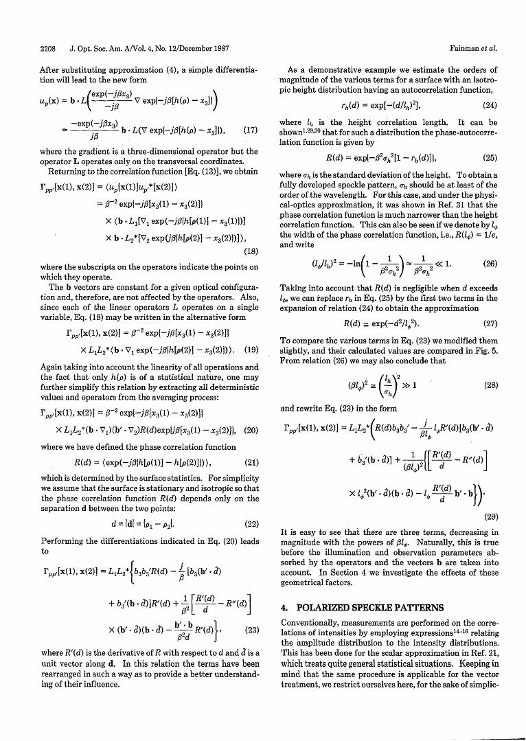
To compare the various terms in Eq. (23) we modified themslightly, and their calculated values are compared in Fig. 5.From relation (26) we may also conclude that
(/31_)2 ( ) >> 1 (28)
and rewrite Eq. (23) in the form
rpp,[x(1), x(2)] = L1 L2*(R(d)b3b3 ' - B lR'(d)[b 3(b' * a)
+ b3'(b * d)] + d R"(d)]
X l 2 (b'. *2)(b a d) - 1 R'(d) b' * b))
(29)
It is easy to see that there are three terms, decreasing inmagnitude with the powers of 61,0. Naturally, this is truebefore the illumination and observation parameters ab-sorbed by the operators and the vectors b are taken intoaccount. In Section 4 we investigate the effects of thesegeometrical factors.
4. POLARIZED SPECKLE PATTERNS
Conventionally, measurements are performed on the corre-lations of intensities by employing expressions'4' 6 relatingthe amplitude distribution to the intensity distributions.This has been done for the scalar approximation in Ref. 21,which treats quite general statistical situations. Keeping inmind that the same procedure is applicable for the vectortreatment, we restrict ourselves here, for the sake of simplic-
Fainman et al.
R(d) =_t 6xp(-d 2/1 02).
Vol. 4, No. 12/December 1987/J. Opt. Soc. Am. A 2209
Additional information may be obtained by choosing b orb' in such a way that its longitudinal component vanishes,eliminating the zero-order terms of Eq. (23) (i.e., the largescalar term). To perform observations one again has tochoose the polarization vector perpendicular to the observa-tion direction, q, as for Eq. (12), reducing the vector b to
b = D X mh = (p2 m3 - p3m2 )xl + (p3 m1 -PlMdC2
+ (pIm 2 - P2mO)X3, (32)
and one can always find a polarization vector such that
.0
Fig. 5. Comparison of the magnitude of the terms in Eq. (23)against the normalized separation, d/Il, for I32ah2 = 10: a, rh(d); b,R(d); c, IR'(d); d, 10f2R'(d)/d; e, l,,2[R"(d) - R'(d)/d].
ity, to circular complex Gaussian statistics, for which theintensity correlation obtains the form
Ip represents the intensity distribution of the scattered fieldobserved through a polarizer having the polarization vector,. The first term, giving the product of the average (overthe ensemble) intensities of two polarizations is a constant,while the degree of correlation is determined entirely by thesecond term, which is the square of the magnitude of theamplitude correlation given in Eqs. (23) and (29).
Returning to Eq. (29), we observe'that all the geometricalfactors involve scalar products of unit vectors that are usual-ly of the same magnitude. This means that in most cases,where b3 or b3' is not very small, the correlation is deter-mined essentially by the first zero-order term:
This relation is simply the requirement that the projectionof D upon a transversal plane (parallel to the object plane) beparallel to the projection of h on the same plane. Repeatingan experiment similar to that of Fig. 6 but satisfying Eq. (33)for one of the polarization directions leads to a correlation(fringe contrast) determined by the derivatives of R(d) rath-er than by the function itself. Returning to Eq. (23), howev-er, one should also consider the operation of L on its argu-ment. Among other things, this operation involves integra-tions that have an effect of averaging. For example, thefirst-order term depends on the projection of d upon b,which averages out to zero for a circularly symmetric aper-ture. As a matter of fact, there is a negligible contributionfor any wide aperture, and one may increase the contribu-tion of this term only by specially designed illuminationstructures. We may conclude that if the zero-order term iseliminated, the correlation will usually be small and willdepend mainly on the second-order term.
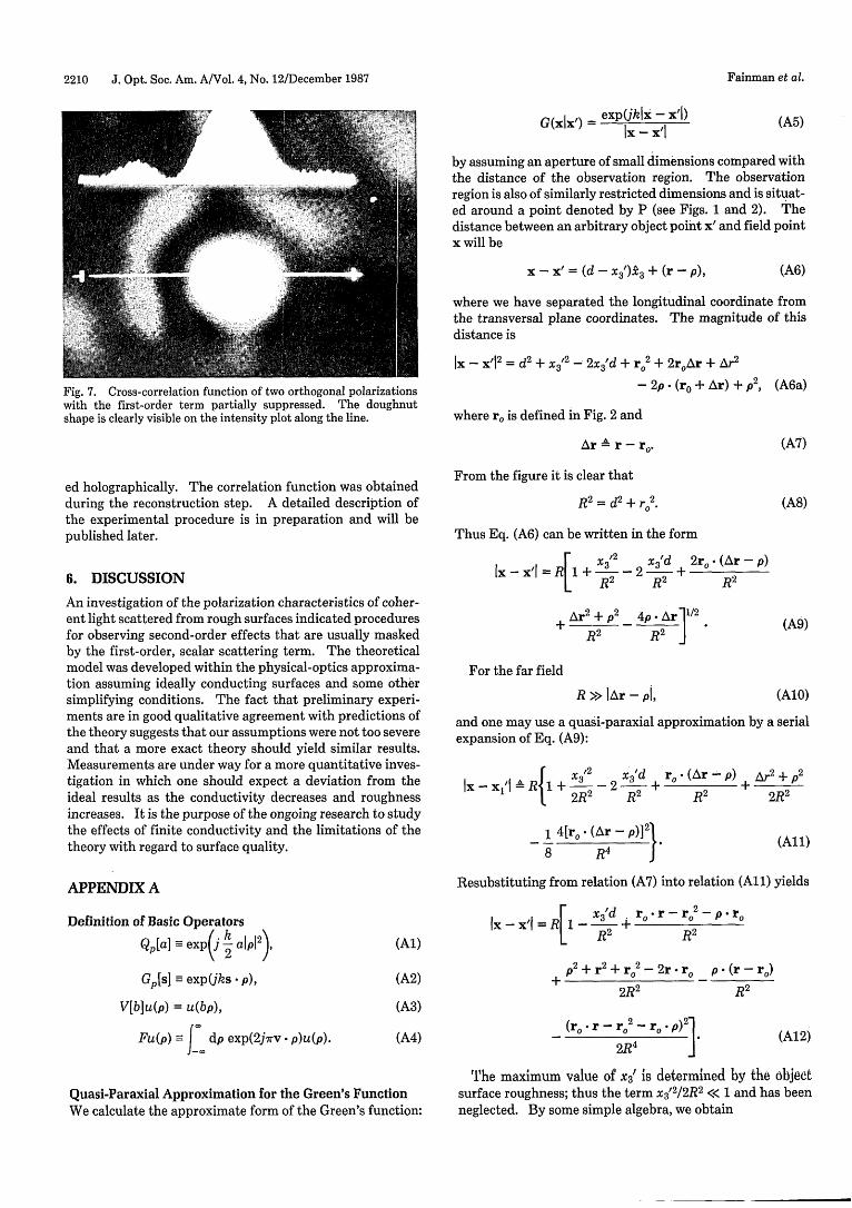
Returning to Fig. 5, we observe that lines b-e representthe various terms of the correlation function [Eq. (23)] withadjusted scales. The first term (line b) corresponds to theusually observed Gaussian shape. The smaller terms (linesc and e), however, vanish at the origin, leading to a dough-nut-shape correlation function.
Figure 7 is a preliminary result showing explicitly thedoughnut-shaped contribution of the second term in Eq.(23). To enhance this term as compared with the first one,the object was illuminated with a grating light structure, andthe two orthogonally polarized speckle patterns were record-
(31)
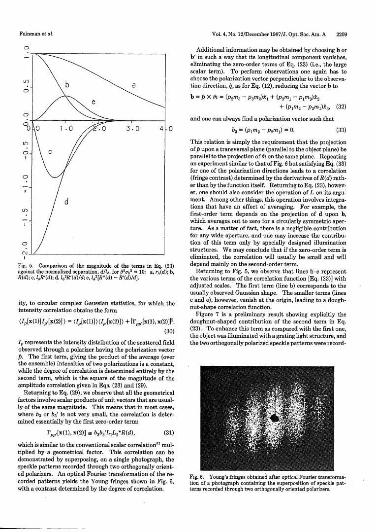
which is similar to the conventional scalar correlation 2 ' mul-tiplied by a geometrical factor. This correlation can bedemonstrated by superposing, on a single photograph, thespeckle patterns recorded through two orthogonally orient-ed polarizers. An optical Fourier transformation of the re-corded patterns yields the Young fringes shown in Fig. 6,with a contrast determined by the degree of correlation.
Fig. 6. Young's fringes obtained after optical Fourier transforma-tion of a photograph containing the superposition of speckle pat-terns recorded through two orthogonally oriented polarizers.
CD
b3 = (plm 2 - p2m) = 0. (33)
Fainman et al.
'L1L *R(d),rpp,[x(l), x(2)] = b3b3 2
2210 J. Opt. Soc. Am. A/Vol. 4, No. 12/December 1987
(A5)G(xlx') = exp(jkix - xl)Ix - X1
by assuming an aperture of small dimensions compared withthe distance of the observation region. The observationregion is also of similarly restricted dimensions and is situat-ed around a point denoted by P (see Figs. 1 and 2). Thedistance between an arbitrary object point x' and field pointx will be
x - x' = (d - x3')3 + (r -p), (A6)
Fig. 7. Cross-correlation function of two orthogonal polarizationswith the first-order term partially suppressed. The doughnutshape is clearly visible on the intensity plot along the line.
where we have separated the longitudinal coordinate fromthe transversal plane coordinates. The magnitude of thisdistance is
Ix - x'12 = d2+ x3
2 - 2x3'd + r02
+ 2r0 Ar + Ar2
-2p * (ro + Ar) + p 2, (A6a)
where r. is defined in Fig. 2 and
Ar r - r,. (A7)
ed holographically. The correlation function was obtainedduring the reconstruction step. A detailed description ofthe experimental procedure is in preparation and will bepublished later.
6. DISCUSSION
An investigation of the polarization characteristics of coher-ent light scattered from rough surfaces indicated proceduresfor observing second-order effects that are usually maskedby the first-order, scalar scattering term. The theoreticalmodel was developed within the physical-optics approxima-tion assuming ideally conducting surfaces and some othersimplifying conditions. The fact that preliminary experi-ments are in good qualitative agreement with predictions ofthe theory suggests that our assumptions were not too severeand that a more exact theory should yield similar results.Measurements are under way for a more quantitative inves-tigation in which one should expect a deviation from theideal results as the conductivity decreases and roughnessincreases. It is the purpose of the ongoing research to studythe effects of finite conductivity and the limitations of thetheory with regard to surface quality.
From the figure it is clear that
= d2 + r 20 (A8)
Thus Eq. (A6) can be written in the form
x3R2 X3Rd + 2r2. (Ar- p)Ix- x'I = R1+ - -2
(A9)+ r2 + p2 4p Ar 1/2
R2 'R2 J
For the far field
R >> lAr-pi, (A10)
and one may use a quasi-paraxial approximation by a serialexpansion of Eq. (A9):
Il A R{1 + X -2 X3 d r-(Arp) 2+p2'R
2 R 2 + R2 + 2R2
8 4[r ( Jr-p)]28 R4 J
(All)
APPENDIX A
Definition of Basic Operators
Qp[a] = exp( 2 alPl2),
Gp[s] - exp(jks * p),
V[b]u(p) = u(bp),
Fu(p) - dp exp(2j7rv * p)u(p).
(Al)
(A2)
(A3)
(A4)
Quasi-Paraxial Approximation for the Green's FunctionWe calculate the approximate form of the Green's function:
Resubstituting from relation (A7) into relation (All) yields
lI-iol=R[l-_+x3d + ro *r-ro2 -p-ro
p2 + r2 + r 2 -2r * ro p * (r-ro)2R2 R2
(r0-r - ro2 -ro p).2R4
(A12)
The maximum value of X3' is determined by the objectsurface roughness; thus the term x3'
2/2R2 << 1 and has beenneglected. By some simple algebra, we obtain
Fainman et al.
Vol. 4, No. 12/December 1987/J. Opt. Soc. Am. A 2211
Ix -x'= R- ~X3 d + p2 + r r,2 p . rix- =R-R +- 2R Rr,4-2r3,P. * r + 2rN3(P0.p) + r0
2r2(pO . p)2 + r02p2(p0 .A)2 - 2r0
2r2(pQ. *p)(pi .P)
2R3, (A13)
where P, PO, and b are unit vectors in the respective directionsof r, r0 , and p (see Fig. 2). Defining an observation angle Oobs
sin 0obs = a = r0/R, (A14)
Eq. (A13) may be written in a more compact form:
Ix-x'I = R- R -3 2° (1 + C2) + [2 [ Ra ° ]
2 2
+p2 1 - Ce2(p, )2 p - r2 R R
-p -[PO.a3_- r a2 (po . p)p9] + C3r * PO. (A15)R
If the same procedure as for the conventional paraxial ap-proximation is used, the denominator of the Green's func-tion does not vary much and can be approximated by R,while in the phase factor we substitute Eq. (A15):
G(xlx')_ const. exp -jk 3 )exp[j k 1 R 2(Po p)2r2]
X exp[j 2 1 °a2 )2 P2Jexp(jk r*P)
X exp{ jk[Pioa3 - R a.2(,o * P)o]* p}exp(jka 3po * r),
(A16)
where all the constant factors (magnitude and phase) havebeen absorbed by the constant. Translating this into opera-tor notation leads to the form
G(xlx') = const. exp( -jk X3 ) Qr [1 - (
X G p(_ r ) QP [1 0t 2(p bo2
V(x)V(x) * G(xlx')J(x') = (VG -V)J + (J * V)VG
+VGX(VXJ)+JX(VXVG)=(J*V)VG, (B2)
where we used the fact that V X VG = 0 and the derivativesof J, which is a function of x' only, vanish identically. Whenthe components of the current, Ji(i = 1, 2, 3), are used, thisexpression has three similar terms:
(J * V)VG = JV d + J2V OG + J3V OG
Reproducing Eq. (6) here, for convenience:
G(xlx') - exptiklx - x'I]jx- x'I
one can perform the calculation for the first term,
V o = Vr(jk - ]
or
(B3)
(B4)
V ddG = (jk- (VG + GV a1X x l)Ox, \.Ix XII\ Ox, Ox,/
-G OIxx V 1Ox' Ix - xT
(B5)
But
VIx - x'I = x - x, = ', (B6)
where we defined the unit vector t in the x - x' direction (seeFig. 2):
VOxxI = 0 VIX-X1 = Ox, Ox, Ox,
iX - X' IX - X12
(B7)
(B8)
and
X Gp[a3po - r aC2(po . p)poJGr(a PO). (A17)
APPENDIX B: DERIVATIVES INVOLVING THEGREEN'S FUNCTION
In the substitution of Eq. (7) into Eq. (5) we are interested inthe operation
V(x)V(x) * J(x')G(xlx'),
VG = (jk- l ,1) GVlx-x'I
= (jk - 1, G) . (B9)
In our far-field approximation,
k >> l 1Ix - X'I(B1)
where we took into account that the integration is performedon x' while the V(x) operates on the x coordinate only.Using vector analysis, we have, by interchanging J and G,
(B10)
and the variation of the direction t with xi is small; thus itcan be neglected together with all the terms of the order Ix -x''-1 or smaller, leaving us with the simple relation
Faimnan et al.
2212 J. Opt. Soc. Am. A/Vol. 4, No. 12/December 1987
V aG k2 IX - x | G&. (B11)ax, ax,
A similar treatment for the other terms of Eq. (B3) results in
(J -V)VG = k2G I + J2 1+ J3 1 )a~ x, OX2 OX3
(B12)
or, collecting all the terms in a vector form,
(J * V)VG 'A -h2 G(J - V*x - x'I)&, (B13)
which, by Eq. (B6) reduces to
(J * V)VG A--k G(J * it (B14)
In the framework of our approximations, & nearly coincideswith q [see Eq. (22)]; thus, returning to expression (Bi), wehave
V(x)V(x) -J(x')G(XIX') A--k 2[j(X,) * q1G, (B15)
and, in dyadic form one may write
VV = -h 2 qq. (B16)
ACKNOWLEDGMENT
This research was partially supported by a grant from theNational Council for Research and Development, Israel, andthe Heinrich Hertz Institute, Berlin, Federal Republic ofGermany.
REFERENCES
1. P. Beckmann, The Depolarization of Electromagnetic Waves(Golem, Boulder, Colorado, 1968).
2. J. C. Leader: "Bidirectional scattering of electromagnetic wavesfrom rough surfaces," J. Appl. Phys. 42, 4808-4816 (1971).
3. I. Ohlidal and F. Lukes, "Ellipsometric parameters of roughsurfaces and of a system substrate-thin film with rough boun-daries," Opt. Acta 19, 817-843 (1972).
4. J. C. Leader, "An analysis of the spatial coherence of laser lightscattered from a surface with two scales of roughness," J. Opt.Soc. Am. 66, 535-546 (1976).
5. K. Gasvik, "The depolarization of light scattered from roughmetal surfaces," Opt. Commun. 22, 61-65 (1977).
6. P. Hariharan, "Statistics of speckle patterns produced by arough metal surface," Opt. Acta 24, 979-987 (1977).
7. J. A. Krill and R. A. Farrell, "Comparison between variational,perturbational, and exact solutions for scattering from randomrough surface model," J. Opt. Soc. Am. 68, 768-774 (1978).
8. F. G. Bass and I. M. Fuchs, Wave Scattering from StatisticallyRough Surfaces (Pergamon, New York, 1979).
9. J. C. Leader, "Analysis and prediction of laser scattering fromrough-surface materials," J. Opt. Soc. Am. 69, 610-628 (1979).
10. K. Nakagawa, T. Nakamura, and T. Asakura: "Effects of polar-ization on the image speckle contrast," Bull. Res. Inst. Appl.Electr. Hokkaido Univ. 31, 20-26 (1979).
11. K. Gasvik, "A theory of polarization-dependent off-specularpeaks of light scattered from rough surfaces," Opt. Acta 27,965-980 (1980).
12. K. Gasvik, "Measurements of polarization dependent off-spec-ular peaks of laser light scattered from rough metal surfaces anddielectrics," Opt. Acta 28, 131-138 (1981).
13. M. Nieto-Vesperinas, "Depolarization of electromagnetic wavesscattered from slightly rough random surfaces: a study bymeans of the extinction theorem," J. Opt. Soc. Am. 72, 539-547(1982).
14. J. W. Goodman, "Some effects of target induced scintillation onoptical random radar performance," Proc. IEEE 53, 1688-1700(1965).
15. J. W. Goodman, "Statistical properties of laser speckle pat-terns," in Laser Speckle and Related Phenomena, J. C. Dainty,ed. (Springer-Verlag, Heidelberg, 1975).
16. J. C. Dainty, "The statistics of speckle patterns," in Progress inOptics, E. Wolf, ed. (North-Holland, Amsterdam, 1976), Vol.XIV.
17. W. H. Carter, "Properties of electromagnetic radiation frompartially correlated current distribution," J. Opt. Soc. Am. 70,1067-1074 (1980).
18. W. H. Carter, "Correlation theory of wavefields generated byfluctuating three dimensional, primary scalar sources. I. Gen-eral theory," Opt. Acta 28,227-244 (1981); "II. Radiation fromisotropic model sources," Opt. Acta 28, 245-259 (1981).
19. M. Nazarathy and J. Shamir, "Fourier optics described by oper-ator algebra," J. Opt. Soc. Am. 70, 150-159 (1980).
20. M. Nazarathy and J. Shamir, "Holography described by opera-tor algebra," J. Opt. Soc. Am. 71, 529-541 (1981).
21. Y. Fainman, J. Shamir, and E. Lenz, "Static and dynamic be-havior of speckle patterns described by operator algebra," Appl.Opt. 20, 3526-3538 (1981).
22. C. T. Tai, Dyadic Green's Functions in ElectromagneticTheory (Intext, San Francisco, Calif., 1971).
23. R. F. Harrington, Time-Harmonic Electromagnetic Fields(McGraw-Hill, New York, 1961).
24. J. D. Jackson, Classical Electrodynamics (Wiley, New York,1975).
25. A. J. Poggio and E. K. Miller: "Integral equation solutions ofthree dimensional scattering problems," in Computer Tech-niques for Electromagnetism, R. Mittra, ed. (Pergamon, Ox-ford, 1973).
26. R. Mittra, "Integral equation method for transient scattering,"in Transient Electromagnetic Fields, L. B. Felsen, ed. (Spring-er-Verlag, Berlin, 1976).
27. S. Silver, Microwave Antenna Theory and Design (McGraw-Hill, New York, 1947).
28. Y. Fainman and J. Shamir, "Polarization of nonplanar wave-fronts," Appl. Opt. 23, 3188-3195 (1984).
29. J. C. Leader, "Incoherent backscatter from rough surfaces: thetwo-scale model reexamined," Radio Sci. 13, 441-457 (1978).
30. W. C. Hoffman, "Scattering of electromagnetic waves fromrough surfaces," Q. J. Appl. Math. 13, 291-304 (1955).
31. H. Stark and Y. Fainman: "Temporal-coherence effects of amoving phase screen illuminated by spatially coherent quasi-monochromatic light," J. Opt. Soc. Am. A 2, 437-444 (1985).