Policy Volatility, Institutions and Economic Growth

Policy Volatility, Institutions and Economic Growth

Antonio Fatas and Ilian Mihov∗

INSEAD and CEPR

Abstract: In this paper we present evidence that policy volatility exerts a strong and directnegative impact on growth. Using data for 93 countries, we construct measures of policyvolatility based on the standard deviation of the residuals from country-specific regressions ofgovernment consumption on output. Undisciplined governments that implement frequent andlarge changes in government spending unrelated to the state of the business cycle generatelower economic growth. We employ both instrumental variables and panel estimation to addressconcerns of omitted variables and endogeneity. A one-standard-deviation increase in policyvolatility reduces long-term economic growth by about 0.74% in the panel regressions, and bymore than one percentage point in the cross-section.

JEL Classification: E60, H11, O11, O57.

∗ We would like to thank the editor and two referees for their comments and sugges-tions. We are grateful for the financial support from INSEAD via research grant 2010-530R.Nicolas Depetris and Rashid Ansari provided excellent research assistance. Address for cor-respondence: Antonio Fatas, INSEAD, Boulevard de Constance, 77305 Fontainebleau, France.E-mail:[email protected].

Policy Volatility, Institutions and Economic Growth 1

I. Introduction

The current economic crisis has generated a renewed interest in the role ofmacroeconomic policy as a stabilizing tool. In particular, fiscal policy is back infashion after years when it was considered as too slow and ineffective. While fiscaland monetary policy can have beneficial short-term effects, there are also reasons toworry about potential adverse long-term effects of policies that are too aggressive.In this paper we focus on fiscal policy and look at one potential long-term cost: ifused too often and at the wrong time, it can generate unnecessary volatility andlower growth.1

The growth literature has already looked at the role of fiscal policy for long-term economic growth. However, it generally considered fiscal policy in levels bylooking at government size, tax rates, and the level of debt. Interestingly, in mostcases the significance of these fiscal policy variables is very low and it disappearsonce the growth regression includes additional controls like the quality of politicalinstitutions. We show that if one considers the volatility instead of the level offiscal policy, there is a robust negative relationship between discretionary changesin government spending and economic growth. This relationship is robust to theintroduction of many control variables, including measures of institutional quality.

Our results are related to two different strands of literature on economicgrowth: one that looks at the link between volatility and growth and one thatstudies the determinants of growth by running a horse race among a large set ofmacroeconomic variables, some of which are related to economic policies.

The relationship between volatility and growth has been studied many timesbefore but the debate is still open. There is evidence of a negative relationshipbetween volatility and growth (Kormendi and Meguire (1985) and Ramey andRamey (1995)) but the evidence is weak. One of the reasons why this relationship

1 Some of the effects of fiscal policy on the economy have been documented in a large bodyof literature. For example, a stream of papers starting with Blanchard and Perotti (2002) haveanalyzed the dynamic effects of fiscal policy on the economy and have produced estimates of theso-called fiscal policy multipliers. Our approach here is different. We also study changes in fiscalpolicy that are unrelated to the state of the business cycle either because they are not timedproperly or because they are motivated by factors other than the macroeconomic conditions inthe country. However, the main goal of the paper is to show that the volatility of these policy

changes exerts a strong negative effect on long-term macroeconomic performance.


might not be as strong as expected is that there could be reverse causality:countries that adopt riskier technologies are countries that grow faster (see Black(1987) for a first reference to this idea and Imbs (2007) for empirical validationof this hypothesis). One way to deal with the problem of reverse causality is toidentify exogenous sources of volatility. By looking at the volatility induced byfiscal policy changes and by using instrumental variables estimation, we avoid theproblem and our results show a much more robust relationship between volatilityand growth than previous studies in this field. In fact, we show that in most of ourspecifications, volatility of output is not a significant explanatory variable, whilepolicy-induced volatility is.

The view that policy volatility is key to long-term economic performance iscertainly not new. In his Nobel laureate lecture, Friedman (1977) points out thatwhile high inflation per se does not change the natural rate of unemployment,an increase in the variance of inflation can generate grave economic inefficienciesand affect the long-term performance of the country by raising its natural rate ofunemployment. Thus long-term monetary neutrality holds when we consider thelevel of policy but not when we look at its volatility.

What is policy volatility? In this paper we construct a measure of policyvolatility based on the variance of unforecastable changes in government consump-tion. We interpret this variance as the aggressiveness with which politicians usespending for reasons other than smoothing the business cycle. Since there areobviously many dimensions of macroeconomic policy, we need to justify our choiceof policy volatility. We start with the idea that in order to estimate the varianceof exogenous shifts in policy stance, we should be able to specify an equation thatresembles a reaction function for every country in our sample. At first, it may seemeasier to do this for monetary policy: Many recent studies have proposed reactionsfunctions with the short-term interest rate as an instrument of monetary policy.This approach, however, leads to some fundamental difficulties: (1) Short-terminterest rates are not available for many countries in our sample, especially for theperiod before 1984; (2) When data are available, the series do not have consistentdefinitions across countries; (3) The interest rate is properly labeled as a monetarypolicy instrument only in few countries, and only since 1984 at best (with the USbeing a notable exception). An alternative approach would be to use monetaryaggregates, but again we face problems with the consistency of definitions. A thirdpossibility would be to use the inflation rate. We decided against this because evena well-specified equation for inflation will inevitably contain shocks that are due


to other factors and not to monetary policy (e.g. oil price shocks, terms of tradeshocks, etc.). As a result we focus on fiscal policy, and by using government con-sumption we can construct an imperfect and yet consistent measure of fiscal policystance. Comparable series for government consumption exist for many countriesand the time span is long enough to allow sensible time-series estimation of thereaction function.2

The second strand of literature that relates to this paper is the one that looksat the deep determinants of economic growth. This strand has recently questionedthe role of macroeconomic policies in determining long-term growth rates. First,policy variables traditionally become insignificant in growth regressions where alarge number of variables are tested as determinants of long-term performance.Second, while policies are very persistent over time, growth rates are not. Andfinally, there is evidence that some of the positive correlation that exists betweengood policies and growth is simply due to the fact that both are the result ofgood institutions, so once we control for the quality of institutions the correlationdisappears.3 In our analysis, we extensively test the robustness of our results byrunning specifications which are similar to those of Acemoglu et al. (2003) orSala-i-Martin et al. (2004). In these specifications, many other institutional andeconomic variables are included to test the robustness of the relationship betweenfiscal policy volatility and growth. The difference between our specification andthose of the previous literature is that while most previous empirical studies usepolicy levels as regressors to predict growth performance, we claim that a keypolicy characteristic that matters for the long-term country performance is thevolatility of policy.4 Thus we argue that it is not enough to attain low inflationand low budget deficits on average, but it is also necessary to have stable inflationand stable fiscal policy.

Using our measure of policy volatility, our findings strongly support the viewthat volatility in policy has a significant negative effect on long-term growth rates.In other words, the way that macroeconomic policy is conducted matters for

2 An alternative measure of policy volatility is to look at the volatility of exchange rates. Thisis the approach of Aghion, Bacchetta, Ranciere and Rogoff (2006) and their results are very much

consistent with the ones presented in our paper.3 One exception is Rodrik (2008a) where the level of the exchange rate is shown to be a

significant determinant of growth.4 Woo (2009) also provides evidence that mismanagement in fiscal policy measured as pro-

cyclical and volatile fiscal policy can harm growth.


growth.

In our analysis, we acknowledge the role of institutions as we uncover a strongrelationship between institutional settings (such as constraints on the executive)and fiscal policy outcomes. In this respect, political institutions that constrainthe executive have a powerful effect on growth by shaping macroeconomic policy.Macroeconomic policy is then the mediating factor through which institutionsaffect growth. By understanding the specific channels through which low-qualityinstitutions affect growth we can provide better recipes for institutional reform asargued by Rodrik (2008b).

But our results also suggest that even within similar institutional settingsdifferences in policy volatility result in different growth rates. This finding isconsistent with the view that policy volatility is determined both by the institutionalenvironment and by shifts in political preferences or other idiosyncratic shocks.

The paper is organized in the following way. Section II describes our empiricalstrategy, the data set and presents the construction of our measure of policyvolatility. Section III reports that in a large cross section of countries higher policyvolatility affects economic growth negatively. In Section IV we construct a panel of10-year averaged data in order to address issues of reverse causality and omittedfixed effects. The link of our results to the empirical and theoretical literature ongrowth is discussed in section V. We conclude the paper by summarizing our mainfindings and by raising some questions for future research.

II. Empirical strategy and data description

To test the hypothesis that policy volatility exerts a negative impact on long-term economic growth we have compiled annual data for 93 countries spanningthe years from 1960 to 2007. We posit that the link between policy volatility andeconomic growth can be identified with the following modification of a standardgrowth regression introduced by Barro (1991):

∆yi = α + λ log(σ�i ) + β�Xi + γ�Zi + ui (1)

In this regression ∆yi is the average growth rate of output per capita (1970-2007) for country i. Our key regressor is the volatility of the exogenous shocks togovernment consumption (σ�

i ). Throughout the paper we will refer to this variableas policy volatility with the obvious caveat that our measure relates only to one


instrument of macroeconomic policy. In equation (1), we also include a vector ofvariables (X) that have been identified as having significant explanatory powerfor the cross-country variation in growth. In order to verify that our key resultsare not due to omitted variables, we will also include other controls captured bythe vector Z. In this section we will discuss the definitions of the main regressorsin equation (1) and the justification for their inclusion. We start first with themeasure of policy volatility.

A. Policy volatility

Our goal is to isolate a measure of policy stance that captures the portion ofdiscretionary fiscal policy that is not explained by the state of the business cycle.Shifts of this kind may occur because of changes in the political preferences of theruling party or because of the desire of the incumbents to generate a temporaryboom before elections.5

In the introduction we explained our focus on fiscal policy by referring to thedifficulties with the estimation of a monetary policy reaction function consistentlyacross countries. In general, several variables can be used to characterize fiscalpolicy. We choose government consumption (as reported in the national incomeand product accounts) because this is the only series that is easily comparableacross countries. Needless to say, this is not a perfect measure — it does notinclude important parts of government spending such as transfers, and it is not acomprehensive measure of fiscal policy because it omits the revenue side. However,the series for the more comprehensive measures like the budget balance, totalexpenditures and total revenues are unreliable as there are frequent breaks andchanges of definitions.6

Equipped with our preferred measure of policy, government consumption, ournext goal is to isolate movements in government consumption that can be consid-ered as policy decisions exogenous to the state of the economy. The literature onfiscal policy uses several approaches to measuring policy volatility. One approach isto calculate raw standard deviations of policy variables (before or after detrending).

5 The literature on the political economy of policy making is enormous. Drazen (2000) andPersson and Tabellini (2000) discuss various models within the political business cycle literature, inwhich politicians have incentives to change spending levels for reasons other than macroeconomic

stabilization.6 The source for the data on government consumption is the World Development Indicators

database of the World Bank. Sources for all the other variables are listed in an appendix.


Another technique is to use GARCH models to construct smooth (time-varying)measures of volatility, which can be used also in panel estimation (as in Henisz,2004). Finally, one can use — as we do — regression analysis to isolate changes infiscal policy that are exogenous to changes in economic conditions. It is straightfor-ward to show that the first two methods do not extract the exogenous componentof policy changes (unless policy is itself exogenous). Therefore, we adopt the thirdapproach, which requires that for each country in our sample we run a regressionof the following type:

∆ln�G

�i,t

= αi + βi,j ∆ln�Y

�i,t

+ �i,t (2)

In these regressions we denote by G real government consumption spending,while Y is real GDP. One possible interpretation of this equation is that of a reactionfunction for the government. Following Alesina, Campante and Tabellini (2008),Lane (2003), Woo (2009), and Aghion, Hemous and Kharroubi (2009) who estimatesimilar policy reaction functions, we estiamte equation (2) by OLS. Of course, weare aware of the possible reverse causality from government spending to outputand we have also estimated several versions of equation (2) using instrumentalvariables.7

We interpret the country-specific volatility of �i,t as an estimate of discretionarypolicy or as a measure of fiscal activism.8 In the calculation of policy volatility werestrict the sample from 1970 to 2007 because we will use data from the 1960s asinitial conditions in the growth regressions.9

7 We have explored two sets of instruments. In a previous version of the paper, we estimatedequation (2) in levels and we instrumented output with a time trend, logarithm of oil prices anda lag of the GDP deflator. In Appendix C on our web sites, we also report results where weuse output in the rest of the world (current and lagged), as well as current and lagged oil pricesas instruments. This is reminiscent of the instruments used by Gali and Perotti (2003) wherethey use foreign output gaps to instrument for domestic output gap. Appendix C also reportsvariations of equation 2 where inflation is included as a control variable. The appendix provides acorrelation matrix between measures of policy volatility derived from various specifications. In allcases, the main results from these robustness checks are consistent with the OLS results presented

in the paper and are available upon request.8 In a recent paper, Aghion and Marinescu (2006) use an alternative measure of budgetary

activism based on the cyclicality of government debt. Their study is focused on understanding

the growth effects of counter-cyclical fiscal policy.9 A recent paper by Koren and Tenreyro (2007) decomposes output volatility in 45 countries

into volatility due to specialization in volatile sectors, volatility due to macroeconomic country-specific shocks, and volatility due to the covariation between sector specific and country-specificcomponents. They interpret the macroeconomic component as resulting from volatile policies or


B. Policy volatility and institutions

Before we proceed to the growth regressions, we investigate whether the newlyconstructed measure is related in any way to the institutional structure of thecountry. Our main institutional variable is Constraints on the executive. We havechosen this variable because a version of this institutional characteristic is used inthe previous literature (e.g. Acemoglu et al (2003)) and also because it shows howmuch freedom the executive has in changing policy stance. The particular variablethat we use takes five values depending on how many checks on the executiveexist. It is calculated as:

Constraints = Legislature + Upper chamber + Judiciary + Federal

Each of the variables on the right-hand side is a dummy variable that takesthe value of 1 for countries that have the specific institutions: Legislature is equalto 1 for countries where the parliament is freely elected and independent of theexecutive; Upper chamber is 1 if the country has a bi-cameral legislature; Judiciary

equals 1 for countries where the judiciary is separated from the executive branch;Federal equals 1 for countries with a federal structure whereby political poweris shared between central and local governments. Thus the variable Constraints

captures potential veto points on the decisions of the executive.10 The data usedto construct Constraints on the executive comes from Henisz (2000).

A variation of our measure of constraints is a variable constructed by Henisz(2000) called ‘political constraints’. This variable differs from our measure intwo ways: (1) the author adjusts for the ideological alignment across politicalinstitutions; and (2) he argues that each additional constraint has a diminishingmarginal effect on policy outcomes and therefore the link between the overallmeasure and the veto points should be nonlinear.11 We prefer to use the simplesum of constraints because it deals in part with the possibility of endogenous

political instability. In an earlier version of this paper, we used their data and we found thattheir measure of country-specific volatility had a correlation of over 0.75 with our policy volatilitymeasure. This result supports their interpretation and also provides evidence that our measure is

not capturing volatility due to the sectoral composition of country’s output.10 The role of veto players in policy-making has been studied extensively in the political econ-

omy literature. See for example Tsebelis (2002) for an insightful discussion of the policy effects of

veto players.11 We have run a nonlinear regression of policy volatility on our measure of constraints. The

nonlinearity was expressed as an exponent of the constraints measure that was estimated by themodel. Somewhat surprisingly the exponent is estimated to be very close to 1, i.e. there is no

strong evidence of non-linearity in the effect of constraints on policy volatility.


response of electoral outcomes (and hence ideological alignment) to economicdevelopments throughout the period.12

There are two other measures of the role of constraints used in the literature.Acemoglu et al. (2003) use Constraints on the executive from the Polity IV dataset. In contrast to our measure which simply records the number of independentveto points, the Polity IV measure is based on interpretation of the effectiveness ofthe veto points. The Database of Political Institutions (DPI) provides a series for avariable called ‘checks’. This variable, as it is the case for the ’political constraints’variable in Henisz (2000), captures not only institutional characteristics in thecountry but also political outcomes as its value is adjusted when, for example, thepresident and the legislature are members of the same party.13

[Insert Table 1 here]

Table 1 documents the institutional determinants of policy volatility. In thefirst column we report that our measure of constraints has a significant negativeeffect on policy volatility. Alone, this institutional characteristic explains 38% ofthe cross-country variation in policy instability. This is a very strong result whichhas a straightforward interpretation – countries with more checks and balances donot allow the executive to change policy for reasons unrelated to the state of theeconomy. Therefore in these countries overall policy volatility is lower.

Column 2 adds as controls three other political and institutional variables usedin the literature as determinants of policy volatility: (1) political system (presidentialvs. parliamentary); (2) electoral system (majoritarian vs. proportional); (3) numberof elections.14 These variables improve the fit of the regression by raising the R2

to 58%. Given that these variables (with the possible exception of the last one) areexogenous to the current state of the economy, we use them later in our analysisas instruments for policy volatility.

In the next two columns we report similar regressions by restricting the sampleto the set of the initially rich countries (column 3) and the set of initially poor

12 The ideological alignment across agents occupying various political institutions can be an

outcome of strategic voting, as Chari et al. (1997) argue.13 Although not reported in the tables below, we have replicated our results using the Polity

IV index, the DPI measure of checks and balances, and the index constructed by Henisz. The

results are available upon request.14 Persson (2005) discusses in detail why the nature of the political and electoral arrangements

might matter for policy outcomes. We refer the reader to his analysis and also to our brief

discussion of the related literature in Section V.


countries (column 4). The cutoff between rich and poor is set at $6,000 GDP percapita (average in 1967-1969), which is close to the mean income in that year.15

With this cutoff, 29 countries are classified as rich and the remaining ones aspoor. The coefficient on constraints is highly significant for poor countries andmarginally significant for the rich ones.16

C. Growth Data and Summary of Controls

In addition to constructing our measure of policy volatility for each country,we have also collected a set of controls that we will use in regression (1) toensure that the link between policy volatility and growth is not due to an omittedvariable. A detailed description of the series is provided in the Data Appendix.Here we offer only a brief overview of the data and the timing assumptions. Inequation (1), the dependent variable (∆yi) is the average growth rate of outputper capita (1970-2007) for country i. The period over which the growth rate iscalculated corresponds to the period over which we construct our measure of policyvolatility. As main controls in equation (1) (vector X) we include five variablesthat have been identified as having significant explanatory power for the cross-country variation in growth. Our choice of controls is based on a recent studyby Sala-i-Martin et al. (2004), who use Bayesian averaging of classical regressionestimates for 67 determinants of growth to identify 18 variables for which theposterior inclusion probability increases relative to the prior. Of these variableswe select four that have clear economic interpretation: (1) Initial GDP per capita;(2) Initial level of human capital; (3) Initial investment price level and (4) Initialgovernment consumption. In addition to these variables, we include in vector X

average openness to control for the effect of trade on economic growth (see Frankeland Romer (1999)). All variables, except initial human capital, are calculated asthe average over 1967-1969, i.e. the three years preceding the start of the growthsample. Initial level of human capital is measured as in Sala-i-Martin et al. (2004)as the percentage of population of relevant age enrolled in primary schools in 1960.The reason for the longer time lag is that those enrolled in primary school willcontribute to growth as workers only after ten or more years.

We choose these five regressors as our main controls because behind eachone of them there is a relatively well-accepted economic theory that explains why

15 The income data is real GDP per capita (chained series) from the Penn World Tables v.6.3.

Earlier version of the paper reports results based on PWT v.6.116 This result is consistent with Aghion et al. (2005).


these variables should predict growth.17 Thus one can explain why initial GDPper capita predicts growth by referring to the neoclassical growth model, but it isvery difficult to provide a theory explaining why, for example, a dummy variabletaking a value of 1 for East Asian countries should predict growth. Furthermore,if the East Asian dummy is indeed so successful in predicting growth, then manytheories would suggest that this predictive power is only temporary — once thecountries from the Asia-Pacific rim reach the technological frontier, their growthrate will slow down and the dummy variable will not be as successful as before.At the same time, GDP per capita will be a predictor (ceteris paribus) as long asthere are countries away from the technological frontier.

While our baseline results include only five controls, we are sensitive to thecriticism that the estimates might be driven by an omitted variable listed amongthe top predictors of growth in Sala-i-Martin et al. (2004). To investigate thesensitivity of our results to changes in the specification of equation (1), we includeadditional controls (vector Z). Within this set we will include sequentially all ofthe top 21 variables from Sala-i-Martin et al. (2004), as well as additional variableslike output volatility, inflation volatility, institutions, etc.

III. Policy volatility and economic growth

A. Baseline Regression

We start by documenting in Figure 1 the correlation between policy volatilityand long-term economic growth over the period 1970-2007. The most volatile fiscalpolicy is recorded in several African countries like Mozambique and Rwanda, whilethe most stable policies are those in the OECD economies. The unconditional rawcorrelation is negative and a regression of growth on policy volatility – reportedin column 1 of Table 2 – yields a negative coefficient of -0.813, which is significantat the 1% level of significance. Taken at face value, this coefficient suggests that acountry like Venezuela — with volatility of fiscal policy close to the mean of thesample — could raise its growth rate by about 0.5% per year if its fiscal policywere stabilized to the same level as Mexico.

[Insert Figure 1 here]


17 For a textbook presentation of the relevant theories see Barro and Sala-i-Martin, 2003.


There are several reasons why we should interpret the scatter plot and theregression results with caution. First, it is possible that our measure of policyvolatility is correlated with some other key determinant of economic growth andtherefore in column 1 the coefficient on policy volatility is biased and inconsistent.Second, the result reported in column 1 could be driven by outliers and hold onlyfor this specific sample. Third, it is possible that policy volatility does dependon recent growth performance and is therefore endogenous to long-term economicgrowth. The rest of Table 2 addresses in part the first two possibilities, while thereverse causality issue is taken up in Table 3.

To check for the possibility that a significant omitted variable is responsible forthe documented link between policy and growth, we include in column 2 five keydeterminants of growth as we discussed in the previous section. We note that all ofthe variables enter with the expected sign: Investment price 1960 and Government

size are not significant, while Initial GDP per capita, Primary enrolment, andOpenness are all significant at the 1% level. The coefficient on our key variable ofinterest – policy volatility – increases in absolute value and remains significant atthe 1% level.

Next, we take up the possibility that the negative effect of policy instabilityon economic growth holds only for this particular sample. In columns 3 and 4we split the sample into rich and poor countries.18 In the poor countries policyvolatility has a bigger impact on long-term growth than in the rich sub-sample.If we test in a nested model for the equality of the two coefficients, however, wefind that the difference is not statistically significant.

A slightly different concern is that we might have misspecified our first stageregression (equation 2) when generating exogenous shocks by running a regressionof government spending on output. It is conceivable that if we do not capturesufficiently well the reaction of fiscal policy to output growth, then a componentof output fluctuations will enter the residuals. Hence, instead of measuring theeffects of policy volatility, we might be documenting the effect of output volatilityon economic growth. A straightforward way to test this claim is to include outputvolatility as a regressor. We report the results in column 5 where we also includethe average inflation and its volatility as controls.19 This modification has no effect

18 As mentioned in the previous section, rich countries are defined as average GDP per capita

in 1967-69 of at least $6,000.19 Monetary variables are included because they can potentially affect both long-term growth

and fiscal policy and therefore our main estimates may suffer from omitted variables bias.


on the coefficient or significance of the policy volatility variable. This suggests thatour measure of policy volatility is not simply a proxy for the volatility of output.The fact that the volatility of output is not in itself significant confirms previousresults in the literature.20

In summary, our measure of fiscal policy volatility enters a standard growthregression with a negative and statistically significant sign. The effects are notnegligible: A reduction in policy volatility corresponding to one standard deviationin our sample raises long-term economic growth by about 0.92 percentage points.

B. Treating policy volatility as endogenous: An IV approach

There are still two potential problems with the results reported in Table 2:omitted variables and endogeneity of policy volatility. It is indeed plausible toargue that an omitted variable may affect both growth and policy volatility, orthat countries with low rates of growth resort more often to aggressive policy inorder to boost demand in the economy (reverse causality). Indeed, this version ofthe reverse causality argument does generate a negative (conditional) correlationbetween output growth and policy volatility. In this section we address theseconcerns by using instrumental variables. Incidentally, instrumental variables willalso help us deal with standard measurement error problems, which might bepresent because of the imprecision with which we have constructed the measure ofpolicy volatility. The presence of measurement error creates an attenuation bias,i.e., it works against finding a significant relationship between policy and growth.If the instruments help us deal with the measurement error we should see anincrease in the absolute value of the coefficient. If, on the other hand, endogeneityhas an important impact on our OLS estimates, then we should see a decrease inthe absolute value of the coefficient on policy volatility.21

From the analysis of the link between institutions and policy volatility in Table1, we know that the constraints on the executive that were in place in 1969, i.e.

20 As pointed out by Imbs (2007) and others, it is conceivable that there is a positive correlationbetween output volatility and growth. Countries that are willing to take more risks might growfaster and, as a result of investing in more innovative and risky technologies, they display higher

output volatility. Similar discussion can be found in Ramey and Ramey (1995).21 Of course, the magnitude of the coefficient could increase in the IV estimation if in the

original regression there is an omitted variable that has positive (negative) correlation with policyvolatility and affects growth in a positive (negative) way. The measurement error is just an

example of such influence.


the year before the start of our sample period, are very good predictors of policyvolatility. In the next battery of tests we use the institutional characteristics ofthe countries in our sample as instruments for policy volatility.


The univariate regression reported in column 1 reveals again the strong negativeimpact of policy volatility on growth. In the next column we add our standardcontrols and the nature of our results does not change. Interestingly, the coefficientestimates for policy volatility in both cases jump relative to the OLS results reportedin Table 2, which is consistent with the presence of measurement error in ourpolicy variable. In columns 3 and 4 we split the sample again into rich and poorcountries and still the coefficient for poor countries remain larger in absolute size.

Column 5 reports results from a perturbation of the baseline IV regression thatalso includes output volatility, inflation and its volatility as regressors. As before, thestandard deviation of output growth is insignificant and the inclusion of monetaryvariables has no impact on the significance of policy volatility. This result showsagain that one cannot attribute our key result to the role of general macroeconomicvolatility for output growth. In both cases the results are consistent with thosedocumented by Sala-i-Martin et al. (2004). Importantly, the coefficient on fiscalpolicy volatility is unaffected in terms of magnitude or statistical significance.22

C. Robustness

We return now to our selection of controls in the growth regression. The studyby Sala-i-Martin et al. (2004) shows that many geographical fixed effects — likea dummy for the East Asian countries or the percentage of the country area withtropical climate — predict growth quite well. Although it is difficult to see whyEast Asian countries would have different policy volatility, i.e. why the omittedvariable is correlated with our measure of policy, we explore later in this sectionhow the most significant regressors from the Sala-i-Martin et al. (2004) study affectour findings.

22 There are always concerns about the validity of instruments in growth regressions. One par-ticular problem occurs when the same instrument has been used in different papers to instrumentfor different growth determinants. In Appendix D we discuss this problem and we use a methoddeveloped by Conley, Hansen, and Rossi (forthcoming) to provide a sensitivity analysis by relaxing

instruments’ exogeneity assumption.


Because our sample period and some of our data sources differ from those usedby Sala-i-Martin et al. (2004), we start our robustness study by using exclusivelydata from their paper. In Table 4, the first column the dependent variable isgrowth from 1960 to 1996 and in addition to our measure of policy volatility, weinclude the controls as they are defined in their study. The fundamental differenceis only that the initial period is 1960 for the controls and dependent variable iscalculated over a different range. The estimation by OLS yields coefficients for thecontrols that are very close to the posterior means reported by Sala-i-Martin etal. (2004), while the coefficient on policy volatility remains close to the estimatesfrom Table 2. Thus the change of the time period and in the exact definition ofthe controls has no effect on our results.


We now proceed by using the top six variables from Sala-i-Martin et al.(2004). We change the range for the dependent variable back to 1970-2007 asin our baseline regression. The top six variables from Sala-i-Martin et al. (2004)are: (1) East Asian dummy; (2) Primary enrolment 1960; (3) Investment price inthe initial period; (4) Initial GDP per capita; (5) Fraction of tropical area; and(6) Coastal population density in the 1960s. Relative to our baseline regressionfrom Table 2, we now drop government consumption and openness and we includethree geographic and demographic characteristics. The OLS regression in column2 shows that the effect of policy volatility on growth is slightly moderated, butit remains significant at the 5% level. The other variables are all significant withthe exception of investment prices.

In the last column of Table 4 we replicate our baseline IV regression byinstrumenting policy volatility with the same instruments as in the previous sectionwhile using the top six controls from Sala-i-Martin et al. (2004). The results remainlargely unaffected with policy volatility still significant at 5%. An alternativeapproach to verify robustness of our results is to add sequentially all of the topeighteen variables from Sala-i-Martin et al. (2004) for which the posterior probabilityof inclusion is higher than the prior. We report the results from these regressionsin Appendix Table B1. In all regressions policy volatility remains significant atbetter than the 5% level.

In summary, we have searched over the space of a large number of variablesthat have been found to determine long-term growth. Our conclusion is that policyvolatility is robustly and significantly correlated with growth. We have not found a


single cross-sectional growth regression that challenges this conclusion. Of course,there might be some suspicion that the instruments are themselves determinants ofgrowth and thus belong to the growth regression as regressors, or that endogeneitycannot be addressed in a satisfactory manner by using cross-sectional regressions.To address some of these concerns we report in the later part of the paper estimatesfrom panel regressions designed to deal with the issue of reverse causality. In thenext section we turn to the marginal explanatory power of our key institutionalvariable – constraints on the executive.

D. The marginal effects of policy volatility and institutions on growth.

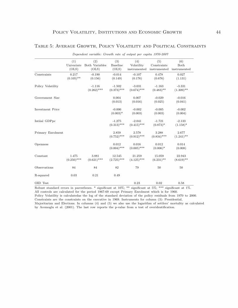
The fact that constraints on the executive affect policy outcomes and thuspolicy volatility is both theoretically justifiable and intuitive. In his book on therole of veto players, Tsebelis (2002) discusses the role of veto points for policystability and summarizes the evidence from a number of studies. The gist of themain argument is that countries with many veto players will have more stableand predictable policy because the process of negotiating new policy initiatives ismore difficult and more costly. So far our results confirm this logic. It is, however,possible that in addition to shaping policy outcomes, constraints on the executivealso exert a direct effect on growth. In this section we ask two related questions:(1) Do political constraints have any additional explanatory power for economicgrowth above the effect they have through policy volatility? (2) Within the sameinstitutional setup, do we observe any effect of policy volatility on growth? Inother words, is the link between volatility and growth fully explained by the waythat policies are shaped by institutions?


Table 5 is devoted to answering the first question. The univariate regressionof output growth rates from 1970 to 2007 on constraints on the executive in 1969show significant positive correlation. A causal interpretation of this result suggeststhat countries with more constraints on the executive achieve faster economicgrowth. But what is the channel? As we have shown in our main tables, oneexplanation is that political constraints lead to more stable policy, which in turncreates a more favorable environment for growth. In column 2 we discover thatthese constraints have no marginal power in explaining growth above and beyondtheir effect on policy stability. Importantly, the coefficient on policy volatility isclose to the estimates from Table 2, where political constraints are excluded. If the


institutional variable was a significant predictor of growth, then not only would weexpect the coefficient on constraints to be significant, but we should also expecta significant change in the estimated effect of policy volatility on growth. Thuswe can conclude that institutions do not affect growth directly and therefore theyare good instruments for policy volatility. This conclusion is confirmed also by theresults in column 3 where we include our standard controls.

Next we want to establish whether institutions have any marginal explanatorypower for growth within the IV framework. In column 4 we include politicalconstraints as a regressor in our baseline IV estimation. Policy is instrumentedonly with the political regime, electoral regime and number of elections. Constraintsremain insignificant while the coefficient on volatility changes in magnitude butremains significant at the 1% level.

One potential criticism of this regression is that constraints themselves areendogenous. Indeed this is the argument that prompted Acemoglu et al. (2003) touse settlers’ mortality rates as an instrument for institutional quality. Their maindependent variable is the level of GDP per capita and therefore in their case onecan plausibly argue that the endogeneity of institutions to past levels of income percapita may create bias in the estimation if both institutions and income per capitaare persistent processes. It is less clear how one can make the same argumentwhen the dependent variable is the subsequent growth rate and initial income percapita is used as a control. Nevertheless, in column 5 we use as an instrumentthe logarithm of settlers’ mortality and we instrument only political constraints.This estimation does not record a significant coefficient for constraints. In the lastcolumn – for completeness – we instrument both policy volatility and politicalconstraints.

In all variations reported in Table 5 we find a statistically significant negativeeffect of policy instability on output growth. At the same time, constraints onthe executive have little additional explanatory power. It is important to interpretthis result correctly. It does not say that institutions do not matter. They do.However, their effect — as one might reasonably expect — is manifested throughpolicy and there is very little (if any) additional impact of political constraints ongrowth.

Now we turn to the second question — whether within the same institutionalsetup policy volatility can make a difference. In the first two columns of Table 6we report OLS regressions for countries where the number of veto points is less


than 2 (column 1) or more than 2 (column 2). Columns 3 and 4 replicate thesame regressions by using our main instruments to instrument for policy volatility.In all cases except for column 2 the results are significant at 5% and indicatethat even within similar institutional frameworks in terms of veto points, policyvolatility matters.23 In the last column we look at the effect of policy volatilitywithin each institutional ‘cell’. First we generate five dummy variables for eachone of the institutional categories (from 0 to 4 constraints) and then interact thesedummies with our policy volatility measure. The coefficients show that withineach institutional structure the volatility of fiscal policy has a negative impact ongrowth. In all cases, except for the case with 4 constraints, the effect is statisticallysignificant. It appears, however, that the impact of policy stability on growth ismuch more pronounced within the low levels of constraints (either dictatorshipsor one veto player systems) than for countries with more developed checks andbalances.24


The results so far lead to potentially important policy recommendation: thereis room for both institutional reform and good macroeconomic policies as recipesfor growth. A simple way to illustrate this point is to look at Table 6. Bothfor the group of countries with low-quality institutions and for those with high-quality ones, the effect of policy volatility on economic growth is negative andsignificant. Thus, Table 6 provides some evidence that even when it is difficultto change institutions, growth performance can be improved by following stablemacroeconomic policies.

IV. Panel estimation

Possibly the most interesting direction for further investigation is the studyof the effects of policy changes on economic growth over time. Ideally, one wouldlike to see how shifts in policy volatility affect growth within a country. Onemight want to use estimation of average treatment effects in order to control

23 We have also estimated regressions for those countries with no constraints at all. We findthat the coefficient on policy volatility remains highly significant and negative. This result notonly confirms the importance of policy stability, but also indicates once again that our findings

cannot be driven by the omission of constraints from the main regression.24 In the last cell, where we have countries with 4 constraints on the executive, we have only 5 ob-

servations. Thus, the large standard errors might be due to the insufficient number of observations.


for observed heterogeneity across countries and to evaluate whether differences inpolicy volatility in otherwise similar countries lead to differences in growth rates.Unfortunately, the estimation of treatment effects is very difficult to implement inour setting. The main reason is that we do not know exactly when treatment —in our case, the shift in policy volatility — has occurred. Despite the difficulties inaddressing the time-variation in our data series, we have attempted to provide atleast a partial view of the robustness of our results using within-country variation.

We start by creating a panel of 10-year averaged data. We have four non-overlapping periods: 1965-1974, 1975-1984, 1985-1994, and 1995-2004. For eachdecade of growth we use as initial conditions data on income per capita, primaryeducation, investment price, government size and openness. These initial conditionsare calculated as averages for the three years preceding the relevant decade.For example, when growth covers the 1985-1994 period, the initial conditionsare calculated as the average from 1982 to 1984. All variables have the samedefinitions as before except primary education. In the cross-sectional regressionswe used primary school enrolment in 1960 because we argued that enrolment in1960 will determine to a large extent the educational level of the population in ourgrowth sample period from 1970 to 2007. In the panel, however, primary schoolenrolment in 1982 to 1984 is clearly a poor predictor for the level of education ofthe labor force from 1985 to 1994. So instead of enrolment we use the percentageof population with primary education.

In Table 7 we present results from this panel by using first pooled OLS.Columns 1 and 2 start by reporting regressions where policy volatility is measuredover the decade period. Focusing on the estimates in column 2, we notice thatthe coefficient on policy volatility is again negative, highly significant but it issomewhat smaller in magnitude compared to our cross-sectional estimate fromTable 2. All of the controls are also highly significant and of the expected sign.


In columns 3 to 7 we report results where policy volatility is lagged oneperiod (one decade). This is an important perturbation of our regression, becauseit deals with the criticism of reverse causality. A skeptic might argue that ourresults in the cross-section or in columns 1 and 2 are driven by the fact thatin a low-growth environment, governments are tempted to try various spendingprograms to jump-start growth. In columns 3, 4 and 5 our baseline regressionuses policy volatility from the previous decade to explain current growth for the


full sample, or from the two groups separated by their income per capita. Theresult is very encouraging for our argument: governments that use fiscal policy tooaggressively and for reasons other than to smooth business cycles, have generatedlower growth in subsequent years. Only for the group of rich countries does theeffect become statistically insignificant, even though it is still negative. Column 6confirms once again that this claim is not due to omitting the overall economicvolatility from the equation.

Although the results are sufficiently robust to every modification of thesepanel equations, it is important to report one particular modification in whichwe include lagged growth rates as regressors. The reason for this inclusion is thefollowing: Current growth rates cannot affect past policy volatility, and yet it is stillpossible that our results are biased if there is reverse causality within the periodand at the same time innovations to growth are highly persistent. In this scenarioa positive innovation to the growth rate may reduce contemporaneously policyvolatility (if there is reverse causality within the period) and raise future growthrates (because of persistence). One way to address this concern is to include laggedgrowth in the estimation. We report the results in column 7. Indeed lagged growthenters with a positive sign and a statistically significant coefficient. Nevertheless,the effect of this modification on the coefficient on policy volatility is minimal.Relative to column 3, the current estimate is marginally lower but its significanceis left virtually intact.

By including lagged growth in the regression we also control to a certainextent for fixed effects that explain cross-sectional differences in growth rates. InTable 8 we document the sensitivity of our key findings to the direct inclusion ofcountry and time fixed effects. Because of the well-known bias in the estimation ofpanel regressions with fixed effects and lagged dependent variable, initially we droplagged growth from the regression.The coefficient is somewhat lower in magnitudebut remains significant when controls are added.


The following three columns include our baseline controls within the panelregression and estimate the model successively with country effects, with time effectsand with both country and time fixed effects. The stability of the coefficient onpolicy volatility is quite remarkable. Among the controls the variable that exhibitsthe most consistent sign and significance is initial GDP per capita. Including outputvolatility as a separate control has no impact on the regression (column 5).


Note that the estimation in Table 8 has used lagged policy volatility as aregressor and therefore one can interpret the results as showing that neither omittedfixed effects, such as geography or weather, nor reverse causality can providea reasonable alternative interpretation. What about reverse causality throughpersistence of growth innovations as an alternative interpretation? In columns 6and 7 we estimate the panel regression by using the Arellano and Bond (1991)methodology, which allows us to include both fixed effects and lagged growth rates.All variables included in the regression are treated as predetermined, which impliesthat they might be correlated with lagged growth rate innovations but they arenot correlated with future growth innovations. The estimation is a two-step GMMusing all available lags of the dependent variable dated before the date of theincluded change in the lagged growth rate as instruments for the change in laggedgrowth. We include two lags of output growth since both lags seem to be highlysignificant. The results are quite telling — in this most demanding specification,policy volatility once again emerges as an important determinant of future changes

in growth rate. The specification tests in the last rows indicate that the conditionsrequired for this method to deliver consistent estimates are present – the test ofoveridentification indicates that there is no correlation between instruments andresiduals, while the test for autocorrelation confirms the presence of a first-ordercorrelation induced by differencing the data.

To sum up the panel estimation, we note that the negative impact of higherpolicy volatility on growth is confirmed in a wide variation of specifications.Even within countries, governments that pursue unstable fiscal policy create anenvironment that harms the subsequent growth performance of the country.

V. Discussion

The research agenda most closely linked to this paper focuses on the relationshipbetween macroeconomic volatility (including policy volatility) and growth. Oneset of papers in this literature looks directly at the relationship between volatilityand growth without focusing on a specific channel through which the effects takeplace. This group includes Ramey and Ramey (1995), Kormendi and Meguire(1985), Imbs (2007), Martin and Rogers (2000), Hnatkovska and Loayza (2005),and Aghion et al. (2005). All of these papers document a negative relationshipbetween overall macroeconomic volatility and economic growth.25

25 Koren and Tenreyro (2007) also document that the volatility of country-specific shocks,


When examining the relationship between volatility and growth there is concernabout omitted variables and reverse causality as there may be factors that driveboth the growth rate and the volatility of the country (as Imbs (2007) argues).To overcome these econometric issues one approach is to identify and isolate anexogenous source of volatility. For example, Alesina et al. (1996) and Dutt andMitra (2008) study the effects of political instability on macroeconomic outcomes,including growth, while Judson and Orphanides (1999) analyze the effects of thevolatility of inflation on growth. Ramey and Ramey (1995) also follow this route byusing fiscal policy changes as an instrument for output volatility. In this respect, ourpaper builds on their approach by focusing on the volatility of discretionary fiscalpolicy as an exogenous source of volatility in the economy. By using instrumentalvariables and also checking a much larger set of controls we provide a more robustset of results.

Aghion et al. (2006) study a different dimension of policy volatility: the effectof exchange rate volatility on productivity growth and their results are consistentwith the results presented in our paper. They find that volatility (of the exchangerate) has a negative effect on growth.

Finally, there is a set of papers that has looked at the effects of alternativedimensions of fiscal policy on growth. Aghion and Marinescu (2006) and Woo(2009) both study the link between the degree of countercyclicality of fiscal policyand growth. In Aghion and Marinescu (2006) less procyclical fiscal policy (“betterfiscal policy”) is associated with higher growth rates of productivity. Woo (2009)presents evidence suggesting that countries that run more procyclical fiscal policyhave lower growth rates. Both of these papers are consistent with our results.Although their policy variables is not volatility, one could establish links betweenthe cyclical stance of fiscal policy and its overall volatility. It is possible that bothmight be affected by the same budgetary processes or institutional variables thatwe use in our instrumental variables estimation; a higher degree of discretion infiscal policy could be linked to more procyclical fiscal policy.

Although our paper is empirical, it is also interesting to understand the link totheoretical models. In endogenous growth models, and from a theoretical point ofview, the relationship between volatility and growth is not an obvious one, as first

which they interpret as policy shocks or political stability, is more important for the overallmacroeconomic volatility in poor rather than in rich countries. Their study relates volatilityto the stages of economic development and thus it is complementary to those studies that link

volatility and growth.


documented in King, Plosser and Rebelo (1988). In a standard neoclassical modelwhere agents (firms) are risk-neutral, investment might increase with uncertainty(at least in prices) because of the convexity of the profit function. The recentmonograph by Aghion and Banerjee (2005) makes this theoretical point within theAK model. There are several ways of modifying the analysis so that volatility anduncertainty become detrimental to investment and long-term growth. The first isvery mechanical and consists of thinking about fluctuations as asymmetric, as inRodrik (1991). The link between volatility and growth could also be happeningthrough uncertainty, as in Feeney (1999). Finally, an endogenous growth modelcan also introduce general equilibrium effects of uncertainty on growth throughinvestment, consumer behavior and the labor supply, as in Aghion et al. (2005),Barlevy (2004), Jones et al. (2005) or de Hek and Roy (2001).

When we turn specifically to policy, we find fewer theoretical papers thatestablish a link between policy volatility and growth. Aizenman and Marion (1993)show that higher policy volatility (modeled as higher dispersion of tax rates) isdetrimental for growth. Hopenhayn and Muniagurria (1996) discuss growth andwelfare effects of policy volatility and persistence within a standard AK model ofgrowth and find that an increase in the frequency of policy changes can lower growth,whereas a greater amplitude of policy changes is associated with higher growthrates. The role of policy volatility can also be detected in Barro (1990), who showsthat growth is a concave function of government size and it is straightforward todemonstrate in his model that an increase in spending volatility will reduce growth.Chong and Gradstein (2006) emphasize a different and, in our view, a plausiblemechanism: In countries where governments cannot commit to a stable tax rate,fewer firms enter into productive industries, which in turn lowers the aggregategrowth rate. Using data from about 80 countries they document a negative effectof policy volatility on firms’ growth rates.

In general, theoretical models emphasize the uncertainty related to the levelof taxes and show that an increase in the variance of tax rates lowers growth.26

Our empirical estimation suggests that volatility of government spending lowersgrowth. One way to link our finding to the theoretical literature on policy volatilityis that an increase in spending volatility implies either concomitant increase in taxrate volatility or, more plausibly, raises the uncertainty about future tax rates,which in turn reduces investment and growth.

26 The fact that higher variance of tax rates has detrimental welfare effects was first emphasized

by Barro (1979).


Our paper also builds on several streams of research that link policy, economicgrowth and institutions. First, following Acemoglu et al. (2003) we explore therole of institutions and policies for economic development. Our main innovationis that we do not consider the level of policy variables (inflation, governmentconsumption, or overvaluation of the exchange rate, i.e., standard macroeconomicpolicy variables) but instead argue that it is policy volatility that is detrimental tomacroeconomic performance. Relative to Acemoglu et al. (2003), we also extendthe analysis to a larger set of countries (not only former colonies). These twopapers belong to a much broader and earlier literature on the effects of institutionson growth or volatility, which is surveyed in the paper by Acemoglu et al.(2004).

Another stream of literature that is related to our paper analyzes the effectsof institutions on macroeconomic policy outcomes. This is a growing field withimportant recent contributions by Persson and Tabellini (2003, 2004) who studyhow constitutional rules shape fiscal policy outcomes. Within this literature severalpapers have specifically looked at the role of constraints in determining policies.The main hypothesis is that governments where power is more concentrated andwhich face fewer veto points are less constrained in the implementation of fiscal andmonetary policy changes. In the case of fiscal policy, there is plenty of empiricalevidence in favor of the idea that constraints matter. Roubini and Sachs (1989)present evidence for OECD economies that governments where power is moreconcentrated create an excessive fiscal policy response to economic shocks. Similarevidence exists for US states. Both Poterba (1994) and Alt and Lowry (1992) showthat divided state governments display a less reactive fiscal policy to changingeconomic conditions. There is also plenty of evidence that veto points in budgetaryprocesses affect fiscal policy outcomes (see Tsebelis (2002)). Talvi and Vegh (2000)present evidence of differences in fiscal policy behavior across countries and examinehow these differences are associated with different political institutions or economicstructures.

VI. Conclusions

Does macroeconomic policy volatility represent a significant determinant ofeconomic growth? Our answer is ‘Yes’. The results documented in this paper showthat the volatility of fiscal policy has a first-order effect on long-term economicperformance. Countries where governments use aggressively discretionary fiscal


policy for reasons not related to the state of the cycle experience a lower rate ofeconomic growth.

This is an important result in light of the recent revival of fiscal policy as atool to manage business cycles. While our results do not question the effectivenessof fiscal policy as a stabilizing tool, they raise some serious concerns about theconsequences of its use. We show that exogenous changes in fiscal policy causeunnecessary output volatility and harm economic growth. Although by constructionthese changes are unrelated to the business cycle and, as such, one might think thatthey are unrelated to countercyclical fiscal policy, there can be a clear connectionbetween the two. First, if the timing of countercyclical fiscal policy is not right, itwill show up in the measure of fiscal policy volatility in our regressions. Second, ifthe asymmetric use of countercyclical fiscal policy leads to accumulation of debt,the government will be required to go through a fiscal consolidation which willalso be captured by our measure of volatility. Of course, our measure of volatilityalso includes changes in fiscal policy which are unrelated to the business cycle,changes that are motivated by political decisions or changes in the agenda of theparty in power.

The fact that macroeconomic policy is an important determinant of economicgrowth runs contrary to some of the recent results in the literature suggestingthat economic policies are simply a proxy for poor institutions and do not have asignificant role even as mediators in this relationship. By measuring macroeconomicpolicy in changes and in levels, as previous papers have done, we show that theresult is robust to the inclusion of a long list of controls, including institutionalvariables. To be clear, we do not deny the role of institutions; indeed we documenthow institutions — and in particular constraints on the executive — shape policyoutcomes. But at the same time we show that economic policies cannot simply beignored. In this respect, while we agree that certain institutions create incentivesfor bad economic policy, we do not conclude that the only way forward is toimprove institutions so that policy improves (and thus leads to higher growth);one can also envision improving policies without changing institutions. In fact, inour sample, policies do vary within the same set of institutions and this variationis robustly related to the subsequent growth of the country. A question for futureresearch is: What drives good fiscal policy above and beyond good institutions?

Finally, it is important to frame our results regarding fiscal policy properlyand within the limits of this analysis. Our findings warn of the potential costsof policy changes. It is, however, conceivable that in certain situations (e.g. fiscal


consolidations), a sharp and unexpected policy change might improve the long-termperformance of the economy. Our results simply imply that policy changes shouldbe implemented carefully, with an appropriate calculation of the long-term effectsstemming from policy instability.


VIII. References

Acemoglu, Daron, Simon Johnson, and James Robinson (2004), “Institutions Asthe Fundamental Cause of Long-Run Growth,” NBER Working Paper 10481.

Acemoglu, Daron, Simon Johnson, James Robinson, and Y. Thaicharoen (2003),“Institutional causes, macroeconomic symptoms: volatility, crises and growth,”Journal of Monetary Economics 50, pp. 49-123.

Aghion, Philippe, Philippe Bacchetta, Romain Ranciere and Kenneth Rogoff (2006),“Exchange Rate Volatility and Productivity Growth: The Role of FinancialDevelopment,” mimeo.

Aghion, Philippe, George-Marios Angeletos, Abhijit Banerjee and Kalina Manova(2005), “Volatility and Growth: Credit Constraints and Productivity En-hancing Investment,” NBER Working Paper 11349.

Aghion, Philippe and Abhijit Banerjee (2005), Volatility and Growth, OxfordUniversity Press.

Aghion, Philippe and Ioana Marinescu (2006), “Cyclical Budgetary Policy andEconomic Growth: What Do We Learn from OECD Panel Data?” manuscript.

Aghion, Philippe Aghion, David Hemous and Enisse Kharroubi (2009), ”CreditConstraints, Cyclical Fiscal Policy and Industry Growth”, manuscript.

Aizenman, J. and N. Marion (1993), “Policy Uncertainty, Persistence and Growth,”Review of International Economics 1(2), 145-163.

Alesina, Alberto, Sule Ozler, Nouriel Roubini and Phillip Swagel (1996), “PoliticalInstability and Economic Growth,” Journal of Economic Growth 1, 189-211.

Alesina, Alberto, Filipe Campante and Guido Tabellini (2008), ” Why is FiscalPolicy Often Procyclical?”, Journal of the European Economic Association, 5,1006-1036.

Alt, James and Robert Lowry (1994). “Divided Governments, Fiscal Institutionsand Budget Deficits: Evidence for the States.” American Political Science

Review, 88.

Arellano, Manuel and Steve Bond (1991), “Some Tests of Specification for PanelData: Monte Carlo Evidence and an Application to Employment Data,” Review

of Economic Studies, 58, 87-97.

Barlevy, Gadi (2004), “The Cost of Business Cycles Under Endogenous Growth,”American Economic Review 94, pp.964-990.


Barro, Robert (1979), “On the Determination of the Public Debt,” Journal of

Political Economy 87, pp.940-971.

Barro, Robert (1990), “Government Spending in a Simple Model of EndogenousGrowth,” Journal of Political Economy 98, pp.103-125.

Barro, Robert (1991), “Economic Growth in a Cross Section of Countries,” Quar-

terly Journal of Economics 106, pp.407-433.

Barro, Robert and Xavier Sala-i-Martin (2003), Economic Growth, The MIT Press.

Bazzi, Samuel and Michael Clemens (2009), “Blunt Instruments: A CautionaryNote on Establishing the Causes of Economic Growth, Working paper 171,Center for Global Development.

Blanchard, Olivier and Roberto Perotti (2002), “An Empirical CharacterizationOf The Dynamic Effects Of Changes In Government Spending And Taxes OnOutput,” The Quarterly Journal of Economics 117(4), pp 1329-1368.

Black, Fischer (1987), Business Cycles and Equilibrium. Basil Blackwell.

Chari, V.V., Larry Jones and Ramon Marimon (1997), “The Economics of Split-Ticket Voting in Representative Democracies,” American Economic Review

87, pp.957-976.

Chong, A. and M. Gradstein (2006), “Policy Volatility and Growth,” manuscript.

Conley, Timothy, Christian Hansen and Peter Rossi (forthcoming), “PlausiblyExogenous”, Review of Economics and Statistics.

Drazen, Allan (2000), Political Economy in Macroeconomics, Princeton: PrincetonUniversity Press.

Dutt, Pushan and Devashish Mitra (2008), “Inequality and the Instability of Polityand Policy,” Economic Journal, August.

de Hek, Paul and Santanu Roy (2001), “On Sustained Growth Under Uncertainty,”International Economic Review, vol. 42(3), pp. 801-814.

Feeney, JoAnne (1999), “International Risk Sharing, Learning by Doing, andGrowth”, Journal of Development Economics, 58, pp. 297-318.

Frankel, J. and David Romer (1999), “Does Trade Cause Growth?” American

Economic Review 89, pp. 379-399.

Friedman, Milton (1977), “Nobel Lecture: Inflation and Unemployment,” Journal

of Political Economy 85, pp. 451-472.


Gali, Jordi and Roberto Perotti (2003), ”Fiscal Policy and Monetary Policy Inte-gration in Europe,” Economic Policy 37, 533-572.

Henisz, Witold J. (2000), “The Institutional Environment for Economic Growth,”Economics and Politics XII, 1-31.

Henisz, Witold J. (2004) “Political Institutions and Policy Volatility,” Economics

and Politics 16.

Hnatovska, V. and N. Loayza (2005) “Volatility and Growth” in J. Aizenman andB. Pinto (eds.) Managing Economic Volatility and Crises: A Practitioner’s

Guide. Cambridge University Press.

Hopenhayn, Hugo A. and Maria E. Muniagurria (1996) “Policy Variability andEconomic Growth,” Review of Economic Studies 63.

Imbs, Jean (2007), “Growth and Volatility,” Journal of Monetary Economics 54(7),pp. 1848-62.

Jones, Larry, Rodolfo Manuelli, Henry Siu and Ennio Stacchetti (2005) “Fluctua-tions in Convex Models of Endogenous Growth I: Growth Effects”, manuscript.

Judson, Ruth, and Atanasio Orphanides (1999), “Inflation, Volatility and Growth,”International Finance 2(1): 117-38.

King, Robert G., Charles I. Plosser and Sergio T. Rebelo (1988), “Production,Growth and Business Cycles, II. New Directions.”Journal of Monetary Eco-

nomics, 21.

Koren, Miklos, and Silvana Tenreyro, (2007) “Volatility and Development,” Quar-

terly Journal of Economics 122(1), 243-287.

Kormendi, Roger, and Philip Meguire, (1985) “Macroeconomic Determinants ofGrowth,” Journal of Monetary Economics 16(2), 141-163.

Lane, Philip (2003), “The Cyclicality of Fiscal Policy: Evidence from the OECD,”Journal of Public Economics 87, 2661-2675.

Martin, Philippe, and Carol Rogers (2000), “Long-Term Growth and Short-TermEconomic Stability,” European Economic Review 44(2), 359-381.

Persson, Torsten (2005) “Forms of Democracy, Policy, and Economic Development,”CEPR Discussion Paper 4398.

Persson, Torsten and Guido Tabellini (2000). Political Economics: Explaining Eco-

nomic Policy. MIT Press.

Persson, T. and G. Tabellini (2003) The Economic Effect of Constitutions. MIT


Press.

Persson, T. and G. Tabellini (2004) “Constitutional Rules and Fiscal Policy Out-comes,” American Economic Review 94, pp. 25-46.

Poterba, James (1994). “State Responses to Fiscal Crises: The Effects of BudgetaryInstitutions.” Journal of Political Economy, 102.

Ramey, G. and V. Ramey (1995), “Cross-Country Evidence on the Link BetweenVolatility and Growth,” American Economic Review LXXXV, 1138-1151.

Rodrik, Dani (1991), “Policy Uncertainty and Private Investment in DevelopingCountries,” Journal of Development Economics 36(2), 229-242

Rodrik, Dani (2008a), “The Real Exchange Rate and Economic Growth,” Brookings

Papers on Economic Activity, 2.

Rodrik, Dani (2008b), “Second-Best Institutions,” American Economic Review,

Papers and Proceedings May.

Roubini, Nouriel and Jeffrey Sachs (1989). “Government Spending and BudgetDeficits in the Industrialized Countries,” Economic Policy, 8.

Sala-i-Martin, Xavier, Gernot Doppelhofer and Ronald Miller (2004), “Determi-nants of Long-Term Growth: A Bayesian Averaging of Classical Estimates(BACE) Approach,” American Economic Review 94, pp. 813-835.

Talvi, Ernesto and Carlos Vegh (2000) “Tax Base Variability and Procyclical FiscalPolicy”, NBER Working Papers No. 7499.

Tsebelis, G. (2002) Veto Players, Princeton University Press.

Woo, Jaejoon (2009), “Why Do More Polarized Countries Run More ProcyclicalFiscal Policy?” Review of Economics and Statistics 91(4), 850-870


Appendix A: Data description

We use annual data for 93 countries over the period 1960-2007. The choice of oursample is dictated by data availability on output and government consumptionwith the requirement that we have at least 20 years of data for each country.

List of CountriesAlgeria Gambia, The NicaraguaAustralia* Germany* NigerAustria* Ghana Norway*Bangladesh Greece* PakistanBelgium* Guatemala PanamaBenin Guinea Papua New GuineaBolivia Guinea-Bissau ParaguayBotswana Honduras PeruBrazil Hong Kong*, China PhilippinesBurkina Faso Iceland* Portugal*Burundi India RwandaCameroon Indonesia SenegalCanada* Ireland* SeychellesCape Verde Italy* SingaporeChad Japan* South Africa*Chile* Jordan Spain*Colombia Kenya Sweden*Comoros Korea, Rep. Switzerland*Congo, Rep. Lesotho Syrian Arab RepublicCosta Rica* Madagascar ThailandCote d’Ivoire Malawi TogoDenmark* Malaysia Trinidad and Tobago*Dominican Republic Mali TunisiaEcuador Mauritania TurkeyEgypt, Arab Rep. Mauritius UgandaEl Salvador Mexico United Kingdom*Ethiopia Morocco United States*Fiji Mozambique Uruguay*Finland* Namibia Venezuela, RB*France* Netherlands* ZambiaGabon* New Zealand* Zimbabwe

The countries with an asterisk are in the group of rich countries with over $6,000income per capita in 1967-69.


Data series used in the country time-series regressions:

Real government consumption — General government final consumption ex-penditure (constant LCU). General government final consumption expenditureincludes all government current expenditures for purchases of goods and services(including compensation of employees). It also includes most expenditures on na-tional defense and security, but excludes government military expenditures that arepart of government capital formation. Data are from World Development Indica-tors. Series identifier in the original data set: General government final consumption

expenditure (constant LCU) (NE.CON.GOVT.KN).

Real GDP — Real GDP in constant local currency units from World Develop-ment Indicators. Series identifier in the original data set: GDP (constant LCU)

(NY.GDP.MKTP.KN).

Price level — GDP deflator from World Development Indicators. Series identifierin the original data set: GDP deflator (NY.GDP.DEFL.ZS).

Index of oil prices — logarithm of petroleum spot price from InternationalFinancial Statistics. Series identifiers in the original data set: Average crude price

(US dollars per barrel, 00176AAZZF...).

Data series used in the cross-sectional regressions:

Real GDP per capita — Real GDP per capita on Purchasing Power Paritybasis from Penn World Tables (version 6.3). Series identifier in the original dataset: rgdpch.

Investment price — Price level of investment on Purchasing Power Parity basisfrom Penn World Tables (version 6.3). Series identifier in the original data set: pi.

Government size — government share of real GDP per capita from Penn WorldTables (version 6.3). Series identifier in the original data set: cg.

Openness — logarithm of the sum of imports and exports as percentage of GDPfrom World Development Indicators, CD-ROM 2002. Series identifier in the originaldata set: Exports of goods and services (percent of GDP) (NE.EXP.GNFS.ZS) andImports of goods and services (percent of GDP) (NE.IMP.GNFS.ZS).

Political system — dummy variable that takes a value of 1 for presidentialregimes and 0 for parliamentary regimes. Data for 51 countries are from Perssonand Tabellini [2001]. Series identifier in the original data set: pres. From theDatabase of Political Institutions (Beck et al. [2000]), for 40 countries. The DPI


variable system is recoded from the original 0, 1, 2 values to a dummy variablethat takes a value of 1 for presidential regimes. Series identifier in the originaldata set: System.

Electoral system — dummy variable that takes a value of 1 for majoritariansystems and 0 for proportional systems. Data for 51 countries are from Persson andTabellini [2001]. Series identifier in the original data set: maj. From the Databaseof Political Institutions for 40 countries. Series identifier in the original data set:Pr.

Number of elections — the average number of elections over the time periodfor which macroeconomic data are available. The series is constructed as the sumof legislative and executive elections from the Database of Political Institutions.Series identifiers in the original data set: legelec and execelec.

Constraints on the executive — from Henisz [2000]. Updated from author’sweb-site. Calculated as the sum of four dummy variables indicating the existence ofgovernment branches independent of the executive. Series identifiers in the originaldata set: L1, L2, J, F.

Primary enrolment — Enrolment rate in primary education in 1960 originallyconstructed by Barro and Lee. Data are posted by Sala-i-Martin et al. (2004) onthe AER web-site.

Log European settler mortality — Log of estimated mortality of Europeansettlers during the early period of European colonization. See Acemoglu et al.(2001) for data description.

Data for Table 4, column 1 is from Sala-i-Martin et al. (2004).


Appendix B: Robustness Using Sala-i-Martin et al. (2004)

To check whether our results are robust to the inclusion of the most significantvariables from Sala-i-Martin et al. (2004), we ran our baseline regression by includingsequentially one of the top 21 variables from their paper. Since we already include4 of these variables as our main controls, the list of new variables contains only17 entries. In all regressions reported in Table B1, we include the main controlsdescribed in the text, policy volatility and one of the 17 variables. To conservespace we report the coefficients only for policy volatility and for the new variable.The estimation is by instrumental variables as described in Table 3.

[Insert Table B1 here]


Appendix C: The effect of endogeneity on the measure ofpolicy volatility

We start with a simple univariate regression (we omit the subscript i). Assumethat all variables are in deviations from the mean:

yt = βxt + ut (C.1)

Suppose that xt is endogenous so that:

E[xtut] = γ

The OLS estimate is biased and inconsistent:

plim�βols = β +γ

σ2x

Thus the variance of the residuals will be:

�σ2u =

1N

T�

t=1

(yt − �βolsxt)2 =1N

T�

t=1

(yt − βxt −γ

σ2x

xt)2 (C.2)

By definition:

σ2u = plim

1N

T�

t=1

(yt − βxt)2 (C.3)

After expanding C.3 and using the definition C.4, we obtain:

�σ2u = σ2

u −γ2

σ2x

(C.4)

Equation C.4 implies that if x is endogenous, then our estimate of volatilitywill be contaminated by a component which is related to the volatility of outputgrowth (the regressor) and the degree of correlation between the errors in equationC1 and output growth.

In the paper we try to deal with this contamination in two ways: (1) bycontrolling for output volatility directly; and (2) by using instrumental variables


estimation in the growth regressions. If the political economy instruments affectoutput volatility only by influencing fiscal policy, then the growth regressions willnot be severely impacted by variations in the fiscal policy reaction function. Inother words, the misspecifications in the reaction function introduce a measurementerror in the volatility estimates. Under standard assumptions, IV estimation inthe growth regression will deal with the biases introduced by measurement errorsand produce consistent and unbiased estimates of the coefficients of interest.


Appendix D: Instrument Validity. Sensitivity Analysis.

While we have provided a large number of robustness tests, there can alwaysbe questions about the validity of our instruments and the possibility that thechannel through which they affect growth could be a different from the one thatwe stress. This is very much the criticism that Bazzi and Clemens (2009) raisefor a variety of papers that use cross-country growth regressions. Solving theendogeneity problem using instrumental variables can only work if the instrumentaffects growth only through the channel that the paper proposes (volatility offiscal policy in our paper). In that sense, using an instrument for more than onemediating channel is incorrect and the associated regressions will produce biasedand inconsistent results. Bazzi and Clemens (2009) illustrate this point by usingseveral empirical studies. The problem can fundamentally be seen as one of omittedvariables: if there is an omitted endogenous variable, which can be instrumentedwith our instruments (Z), then the instruments will be correlated with the errors;hence the argument that researchers cannot use the same instrument in regressionswith the same dependent variable instrumenting for different endogenous variables.One can reduce this problem to the following simple set-up with two endogenousvariables and one instrument. Suppose that the true regression is:

Y = βX + αW + � (D1)

Assume that both X and W are endogenous and Z is a valid instrumentfor both (i.e. orthogonal to the errors and highly correlated with X and W ).Because we have one instrument for two endogenous variables, it is impossible toidentify the effect of each of these variables on Y . Often this simple problem isoverlooked when W is excluded from the regression, and the researcher uses Z asan instrument for X to estimate:

Y = βX + ν (D2)

Since ν = αW + � and E[Z �W ] �= 0 , the IV regression is invalid.

There is a parallel between this problem and that of omitted variables in astandard OLS regression. Even if X and W are exogenous, omitting one of themcould produce biased results in the estimation of the equation above (as long asthey are not orthogonal). The literature on economic growth over the last decade


can be seen as an ongoing race to include an increasing number of controls in theregression to minimize the risk of an omitted variable bias.

In our setting, a skeptic might argue that there is an omitted endogenousvariable, which is also correlated with our main instrument (political constraints).What do Bazzi and Clemens (2009) recommend in this case? In their concludingremarks, they make two recommendations relevant to our paper:

(1) “Generalize the theoretical underpinnings of an instrument to account for

other published results with the same instrument.” Although we do not provide aspecific model, from a theoretical point of view the number of veto points can beeasily linked to fiscal policy volatility. An extensive literature has looked at theconnection between budget processes, institutions, and fiscal policy outcomes.27

We believe that what we are presenting is a very specific channel through whicha certain institutional set-up (number of veto points) affects growth. But whatmatters is whether there are other potential channels — different from policyvolatility — through which veto points affect economic growth. Following Bazziand Clemens’s suggestion, we have completed a thorough search of the papers thatcite Henisz’s work (our measure of constraints is borrowed from his work). Whilehis index has been used in many papers, we did not find a single paper wherepolitical constraints, as measured by Henisz, have been used as an instrument ina growth regression. This finding offers at least a minimum level of reassurancethat we are not using an instrument, which had been used by others to explore thevalidity of another growth channel. In other words, there is no obvious omittedvariable in the literature that could be a mediating channel in the regression we arerunning. Still, the fact that no one else has written a paper using this particularinstrument does not rule out that such a variable exists. It is also possible that ourinstrument is correlated with another instrument that is in turn correlated with anomitted variable. To address these concerns we follow the second recommendationof Bazzi and Clemens (2009).

(2) “Deploy the latest tools of probing validity.” In particular, they mentionseveral recent papers which propose different methods for sensitivity analysis whenusing instrumental variables. We borrow the set-up from Conley, Hansen and Rossi

27 One recent example is Alesina, Campante and Tabellini (2008). They provide a model toexplain fiscal policy outcomes and make use of the political constraints variable that we use in oneof their specifications. A second example, also close to our empirical specification, is Woo (2009).More generally, Persson and Tabellini (2002) offer a general discussion of the role of checks and

balances, separation of powers, and appropriate budgetary procedures.


(forthcoming), henceforth referred to as CNR, to present our sensitivity analysis.Going back to equation (D1) above: Suppose that the projection of W onto Z isθZ. Then in regression (D1), we can substitute for W its projection and generatethe following regression:

Y = βX + γZ + ξ (D3)

This equation is listed (in matrix form) as equation (1) in CNR. In this regression,Z will be a valid instrument for X, in the sense that it will be uncorrelated withthe error term. Of course, we cannot estimate this equation because Z is botha regressor and an instrument. The standard IV regression assumes that γ = 0.CNR suggest relaxing this assumption and exploring how the estimate of the maincoefficient of interest, β, varies when γ deviates from zero.

CNR propose three different methods for sensitivity analysis. We use the so-called Union of Confidence Intervals method. In terms of coverage, as CNR pointout, this is the most conservative interval estimate for the parameter of interestβ. The method is based on the assumption that the researcher knows the supportof γ, G. If the true value of γ is denoted by γ0 ∈ G, then we can estimate β

consistently by using Z as an instrument for X in the following regression:

(Y − γ0Z) = βX + ξ (D4)

The essence of this method is to obtain a (1−α) confidence interval for β conditionalon a specific γ0 ∈ G, and then to construct the confidence interval for β as theunion of all confidence intervals for γ0 ∈ G. This union of confidence intervals willbe quite large but it will cover the true parameter value with a probability of atleast (1 − α). The difficult question is to determine the support of γ. We followone of the examples from CNR by selecting a range linked to the key coefficient ofinterest. We let γ0 ∈ [−δβ, δβ], where β is the coefficient on policy volatility. Wetake the regression from Table 3, column 2 as our baseline. For this regression theestimate of β is -2.90. We focus on our main instrument political constraints and,following CNR’s example of demand for margarine, we allow the “indirect effect”of political constraints to be at most 30%. So, we vary δ from 0 to 0.3. This impliesthat the union of confidence intervals is constructed for γ0 ∈ [−0.87, 0.87]. Thereis one issue that is not easy to resolve: the interpretation of this range. Is it wideenough? The problem is that without having a detailed perspective on what theadditional channel is, the variance of the omitted variable or its correlation withthe instrument, it is impossible to provide a straightforward interpretation of this


range. If we had a specific channel or an omitted variable in mind, this exercisecould be even more meaningful. We still find this analysis quite useful becauseit shows that for some deviations from the assumption of pure exogeneity, theeffect of policy volatility on growth remains negative and significant. The dashedlines in Figure 2 represent the lower and upper bounds for the union of confidenceintervals, where the confidence interval for each specific γ0 has coverage of 95%.

[Insert Figure 2 here]

It is clear that at some point the union of confidence intervals will include zeroand the null of no effect will not be rejected. This observation, however, applies toany instrumental variables regression. But the main contribution of the sensitivityanalysis is to show that mild relaxation of the excludability restriction does notinvalidate our inference completely.

To sum up, Bazzi and Clemens (2009) argue that in order to produce moreconvincing results researchers should account for the findings in the literature,provide theoretical arguments to include both new and old results, and carry outsensitivity analysis. We think that these points can be linked together: If a variablehas a clear theoretical justification, the range for the sensitivity analysis can bereduced. The link between veto points and fiscal policy volatility is quite strongand obvious; hence we think that the sensitivity analysis performed is informative.Of course, in this methodology one will never have definitive evidence that rulesout the existence of other effects. The usefulness of our exploration is that it showsthat the additional effect must be very strong in order to overturn our findings.


Table 1. Institutions and Policy VolatilityDependent variable:Policy Volatility 1970-2007

(1) (2) (3) (4)

Univariate Baseline Rich Poor

Constraints on -0.365 -0.234 -0.143 -0.191

the Executive (0.046)*** (0.046)*** (0.070)* (0.085)**

Presidential 0.759 0.736 0.294

(0.139)*** (0.194)*** (0.254)

Majoritarian -0.122 0.081 -0.378

(0.116) (0.202) (0.155)**

Elections -1.469 -1.079 -1.182

(0.439)*** (0.635) (0.516)**

Constant 2.161 2.036 1.485 2.471

(0.084)*** (0.191)*** (0.246)*** (0.286)***

Observations 83 81 29 52

R-squared 0.38 0.58 0.40 0.28

Robust standard errors in parentheses.

* significant at 10%; ** significant at 5%; *** significant at 1%


Table 2. Average Growth and Policy VolatilityDependent variable: Growth rate of output per capita 1970-2007

(1) (2) (3) (4) (5)

Univariate Baseline Rich Poor Additional

Controls

Policy -0.813 -1.358 -0.585 -1.558 -1.011

Volatility (0.153)*** (0.356)*** (0.274)** (0.459)*** (0.362)***

Government -0.001 -0.066 0.007 -0.000

Size (0.013) (0.019)*** (0.014) (0.013)

Investment -0.003 -0.006 -0.003 -0.003

Price (0.003) (-0.004) (0.005) (0.003)

Initial -1.195 -0.719 -1.381 -1.232

GDPpc (0.277)*** (0.475) (0.370)*** (0.269)***

Primary 2.806 -0.526 2.896 3.153

Enrolment (0.732)*** (4.268) (0.800)*** (0.691)***

Openness 0.011 0.006 0.01 0.01

(0.004)*** (0.005) (0.006)* (0.004)**

Output -0.427

Volatility (0.412)

Inflation -0.02

(0.017)

Variance of 0.000

Inflation (0.000)

Constant 3.169 11.599 11.065 13.233 11.923

(0.268)*** (2.514)*** (6.426)* (3.297)*** (2.512)***

Observations 93 87 30 57 87

R-squared 0.16 0.45 0.57 0.45 0.49


* significant at 10%; ** significant at 5%; *** significant at 1%

All controls are calculated for the period 1967-1969 except Prim. Enrolment

calculated for 1960-1964. Policy Volatility is calculated as the log of the

standard deviations of the policy residuals from 1970 to 2007.


Table 3: Average growth and policy volatility:

Instrumental Variables EstimationDependent variable: Growth rate of output per capita 1970-2007

(1) (2) (3) (4) (5)

Univariate Baseline Rich Poor Additional

Controls

Policy -1.094 -2.902 -1.791 -2.871 -3.378

Volatility (0.234)*** (0.643)*** (0.838)** (0.966)*** (1.211)***

Government 0.005 -0.054 0.015 0.002

Size (0.014) (0.038) (0.015) (0.015)

Investment -0.002 -0.002 -0.006 -0.003

Price (0.003) (0.003) (0.006) (0.003)

Initial -2.066 -1.516 -2.036 -1.965

GDPpc (0.393)*** (0.708)** (0.455)*** (0.418)***

Primary 2.597 1.351 2.606 2.304

Enrolment (0.885)*** (7.955) (0.937)*** (1.217)*

Openness 0.016 0.009 0.015 0.014

(0.005)*** (0.009) (0.005)*** (0.005)**

Output Volatility 1.079

(0.992)

Inflation -0.012

(0.024)

Variance of 0.000

Inflation (0.000)

Constant 3.603 21.159 17.261 21.028 20.141

(0.426)*** (4.035)*** (9.954)* (4.772)*** (4.365)***


OID Test 0.01 0.81 0.85 0.73 0.86

Robust standard errors in parentheses. * significant at 10%; ** significant at 5%;

*** significant at 1%. All controls are calculated for the period 1967-69

except Primary Enrolment which is for 1960. Policy Volatility is calculated

as the log of the standard deviation of the policy residuals from 1970 to 2007.

Instruments for policy volatility: Constraints in 1969, Presidential, Majoritarian and

Elections. The last row reports the p-value from a test of overidentification.


Table 4: Robustness: Sala-i-Martin et al. (2004) VariablesDependent variable: Growth rate of output per capita 1970-2007

(1) (2) (3)

Using Sala-i- Top 6 Top 6

Martin et al. (OLS) (IV)

Data

Policy Volatility -1.373 -0.835 -2.309

(0.279)*** (0.365)** (0.873)**

Investment Price -0.004

-0.004

Government Size -5.88

(2.020)***

Initial GDPpc -1.294

(0.288)***

Primary Enrolment 2.816

(0.651)***

Openness 1.326

(0.443)***

Investment Price -0.002 0.000

(0.002) (0.003)

Initial GDPpc -1.042 -1.705

(0.249)*** (0.463)***

Primary Enrolment 2.426 2.324

(0.656)*** (0.766)***

East Asian 1.103 0.627

(0.554)** (0.810)

Tropical Area -0.917 -0.192

(0.301)*** (0.591)

Population Coastal Area 0.001 0.001

(0.000)*** (0.000)***

Constant 12.16 10.449 18.009

(2.377)*** (2.407)*** (4.812)***

Observations 85 85 78

R-squared 0.6 0.57

OID test 0.93


* significant at 10%; ** significant at 5%; *** significant at 1%.

In the first column we use data from Sala-i-Martin et al. (2004)

The dependent variable in this column is for the period 1960-69.

In columns (2) and (3) we use the same data as in Tables 2 and 3.

Initial GDPpc and Investment Price are calculated for the period

1967-69. Primary Enrolment is for 1960. The remaining controls

are as defined by Sala-i-Martin et al. (2004), see also Data Appendix.

Policy Volatility is claculated as the standard deviations of the policy

residuals from 1970 to 2007. Instruments for Policy Volatility:

Constraints in 1969, Presidential, Majoritarian and Elections.

The last row reports the p-value from a test of overidentification.


Table 5: Average Growth, Policy Volatility and Political Constraints

Dependent variable: Growth rate of output per capita 1970-2007

(1) (2) (3) (4) (5) (6)

Univariate Both Variables Baseline Volatility Constraints Both

(OLS) (OLS) (OLS) instrumented instrumented instrumented

Constraints 0.217 -0.190 -0.014 -0.107 0.478 0.027

(0.105)** (0.156) (0.149) (0.176) (0.676) (1.131)

Policy Volatility -1.116 -1.502 -3.031 -1.163 -3.331

(0.262)*** (0.373)*** (0.674)*** (0.483)** (1.309)**

Government Size 0.004 0.007 -0.029 -0.016

(0.013) (0.016) (0.025) (0.041)

Investment Price -0.006 -0.002 -0.005 -0.002

(0.003)* (0.003) (0.003) (0.004)

Intiial GDPpc -1.275 -2.041 -1.721 -2.133

(0.313)*** (0.415)*** (0.873)* (1.158)*

Primary Enrolment 2.859 2.578 3.288 2.677

(0.752)*** (0.912)*** (0.834)*** (1.241)**

Openness 0.012 0.016 0.012 0.014

(0.004)*** (0.005)*** (0.006)* (0.008)

Constant 1.475 3.881 12.545 21.259 15.059 22.943

(0.250)*** (0.621)*** (2.725)*** (4.125)*** (6.231)** (8.619)**

Observations 84 84 82 79 50 50

R-squared 0.03 0.21 0.49

OID Test 0.23 0.02 0.58

Robust standard errors in parentheses. * significant at 10%; ** significant at 5%; *** significant at 1%.

All controls are calculated for the period 1967-69 except Primary Enrolment which is for 1960.

Policy Volatility is calculatedas the log of the standard deviation of the policy residuals from 1970 to 2000.

Constraints are the constraints on the executive in 1969. Instruments for column (3): Presidential,

Majoritarian and Elections. In columns (4) and (5) we also use the logarithm of settlers’ mortality as calculated

by Acemoglu et al. (2001). The last row reports the p-value from a test of overidentification.


Table 6: The Effect of Policy Volatility

within Institutional StructureDependent variable: Growth rate of output per capita 1970-2007

(1) (2) (3) (4) (5)

Constr. < 2 Constr. >= 2 Constr. < 2 Constr. >= 2 with dummies

(OLS) (OLS) (IV) (IV) (OLS)

Policy Volatility -1.835 -0.387 -2.559 -1.713

(0.428)*** (0.318) (1.087)** (0.618)**

Government Size 0.022 -0.054 0.019 -0.03 -0.004

(0.014) (0.012)*** (0.031) (0.014)** (0.016)

Investment Price -0.009 0 -0.005 0.002 -0.009

(0.004)** (0.002) (0.005) (0.003) (0.004)**

Initial GDPpc -1.452 -0.574 -1.735 -1.475 -1.452

(0.317)*** (0.469) (0.507)*** (0.778)* (0.322)***

Primary Enrolment 2.986 -1.558 2.716 -0.191 3.015

(0.805)*** (2.228) (0.935)*** (2.944) (0.765)***

Openness 0.011 0.016 0.013 0.021 0.013

(0.006)* (0.007)** (0.006)** (0.010)** (0.005)***

d0 14.194

(2.990)***

d1 15.322

(2.603)***

d2 13.504

(3.021)***

d3 13.344

(2.843)***

d4 13.517

(4.184)***

d0*Policy Volatility -1.48

(0.510)***


(0.361)***


(0.401)**


(0.366)**


(3.519)

Constant 14.428 9.363 17.977 17.032

(2.764)*** (3.437)** (5.859)*** (5.047)***


R-squared 0.56 0.59 0.82

OID Test 0.05 0.71

Robust standard errors in parentheses. All regressions include an intercept.

significant at 10%; ** significant at 5%; *** significant at 1%. All controls are calculated

for the period 1967-69 except Primary Enrolment which is for 1960. Policy Volatility is

calculated as the log of the standard deviation of the policy residuals from 1970 to 2007.

Instruments for Policy Volatility: Constraints in 1969, Presidential, Majoritarian and Elections.

The dummies d0-d4 in the last column are defined as: d0 is equal to 1 for countries with no

constraints, d1 is equal to 1 for countries with 1 constraint, etc. The last row reports

the p-value from a test of overidentification.


Table 7: Panel Estimation I, Pooled OLS

Dependent variable: Growth rate of output per capita by decades: (1965-74, 1975-1984, 1985-1994, 1995-2004)

(1) (2) (3) (4) (5) (6) (7)

Univariate Baseline With lagged Rich Poor With output With lagged

volatility volatility growth

Policy -0.678 -0.918

Volatility (0.150)*** (0.279)***

Lagged Policy -1.042 -0.343 -1.294 -0.976 -0.957

Volatility (0.274)*** (0.453) (0.356)*** (0.294)*** (0.264)***

Initial GDPpc -1.152 -1.086 -0.565 -1.073 -1.110 -1.207

(0.286)*** (0.306)*** (0.808) (0.369)*** (0.309)*** (0.313)***

Primary 3.262 3.064 3.171 2.996 3.075 3.360

Schooling (0.817)*** (0.939)*** (2.216) (1.040)*** (0.944)*** (0.945)***

Openness 0.011 0.011 0.009 0.011 0.012 0.01

(0.003)*** (0.003)*** (0.006) (0.003)*** (0.003)*** (0.002)***

Government -0.05 -0.056 -0.056 -0.052 -0.054 -0.044

Size (0.025)** (0.022)** (0.045) (0.025)** (0.022)** (0.023)*

Investment -0.006 -0.001 -0.010 0.000 -0.001 0.000

Price (0.003)* (0.004) (0.007) (0.005) (0.004) (0.004)

Lagged 0.167

Growth (0.070)**

Lagged Output -0.060

Volatility (0.116)

Constant 2.821 11.602 10.856 5.874 11.109 11.084 11.081

(0.226)*** (2.460)*** (2.578)*** (7.131) (3.039)*** (2.595)*** (2.609)***

Observations 351 292 221 86 135 221 221

R-squared 0.06 0.20 0.18 0.14 0.18 0.18 0.21


The dependent variable and policy volatility are calculated for the periods 1965-74, 1975-1984, 1985-1994

and 1995-2000. When lagged policy volatility is used it is the policy volatility for the previous decade. The

controls are calculated for the three-year periods preceeding the decade for which the growth rate is calculated.


Table 8: Panel Estimation II, Controlling for Fixed EffectsDependent variable: Growth rate of output per capita by decades: (1965-74, 1975-1984, 1985-1994, 1995-2004)

(1) (2) (3) (4) (5) (6) (7)

Univariate Baseline Baseline With time Output Vol. Arellano Bond Arellano Bond

country country time and country time and estimator estimator with

effects effects effects effects country effects time effects

Lagged Policy -0.172 -0.921 -1.032 -0.857 -0.867 -1.033 -0.730

Volatility (0.323) (0.323)*** (0.278)*** (0.299)*** (0.300)*** (0.189)*** (0.195)***

Initial GDPpc -5.219 -1.050 -6.506 -6.478 -3.813 -4.304

(0.707)*** (0.306)*** (0.710)*** (0.713)*** (0.227)*** (0.360)***

Primary 9.418 2.876 1.308 1.213 2.447 -0.453

Schooling (2.005)*** (0.921)*** (2.449) (2.459) (1.171)** (1.225)

Openness 0.018 0.011 0.015 0.015 0.014 0.015

(0.011)* (0.003)*** (0.010) (0.010) (0.004)*** (0.004)***

Government -0.016 -0.058 -0.040 -0.042 -0.049 -0.033

Size (0.038) (0.022)*** (0.037) (0.037) (0.019)*** (0.016)**

Investment 0.008 -0.002 0.011 0.011 -0.005 0.000

Price (0.009) (0.004) (0.008) (0.008) (0.002)** (0.003)

Lagged Output 0.036

Volatility (0.060)

Lagged -0.297 -0.256

Growth (0.027)*** (0.044)***

Lagged -0.231 -0.129

Growth (2nd) (0.034)*** (0.040)***

Constant 1.647 40.525 11.069 58.225 57.985 35.981 41.471

(0.547)*** (5.762)*** (2.576)*** (6.481)*** (6.509)*** (2.234)*** (2.701)***

Country Effects Yes Yes No Yes Yes Yes Yes

Time Effects No No Yes Yes Yes No Yes

Observations 259 221 221 221 221 143 143

Number of 93 78 78 78 78 77 77

Countries

R-squared 0.00 0.32 0.19 0.43 0.43

OID Test 0.114 0.100

1st Order Serial 0.004 0.005

Correlation


The dependent variable and policy volatility are calculated for the periods 1965-74, 1975-1984, 1985-1994

and 1995-2000. When lagged policy volatility is used it is the policy volatility for the previous decade. The

controls are calculated for the three-year periods preceeding the decade for which the growth rate is calculated.


Appendix Table B1: Average Growth and Policy Volatility (controlling

for Sala-et-Martin et al. variables). IV estimation.Dependent variable: Growth rate of output per capita 1970-2000

(1) (2) (3)Included Control Coefficient on Coefficient on

the marginal policy R2

variable volatility

East Asian dummy -2.685 0.768 0.41(0.686)*** (0.723)

Fraction of tropical area -2.84 -0.244 0.37(0.792)*** (0.564)

Population density coastal 1960s -2.69 0.001 0.41(0.735)*** (0.001)

Ethnolinguistic fractionalization -2.994 0.461 0.33(0.672)*** (0.391)

Real exchange rate distortions -2.434 -0.001 0.47(0.753)*** (0.004)

Population density 1960 -2.907 0.001 0.38(0.635)*** (0.000)***

Fraction speaking foreign language -3.063 -1.143 0.38(0.662)*** (0.694)

Fraction Buddhist -3.407 0.618 0.25(1.107)*** (0.764)

Fraction Muslim -2.821 1.012 0.39(0.580)*** (0.546)*

Years open -2.752 0.215 0.39(0.778)*** (1.083)

Spanish colony -2.849 -0.167 0.37(0.891)*** (0.367)

Fraction GDP in mining -2.964 3.058 0.37(0.642)*** (1.304)**

Latin American dummy -2.795 0.596 0.38(0.706)*** (0.664)

African dummy -2.994 -1.224 0.37(0.666)*** (0.363)***

Fraction Confucian -2.685 3.607 0.43(0.603)*** (0.833)***

Life expectancy in 1960 -2.837 0.051 0.37(0.667)*** (0.028)*

Malaria prevalence in 1960s -3.311 -0.649 0.27(0.739)*** (0.584)

Robust standard errors in parentheses. * significant at 10%;** significant at 5%; *** significant at 1%.

POLICY VOLATILITY, INSTITUTIONS AND ECONOMIC GROWTH !"#

####

#

!"#$!"%$

&'($

&)*$

&)+$

&,!$&-'$

&.*$

&/!$

&0!$

1!+$

12)$

12*$

1(3$

14/$

1.-$1.*$

1.4$

153$

1/($')"$'+6$

'.4$

'7!$

)1"$

)-8$)#5$

)%2$

,(+$

,9($,/!$

-!&$

-&/$

-2!$

-(+$-4&$

-+&$

-/1$

-%4$

26-$

2+'$

('+$

(+'$

(/*$

(#*$

(%!$

9./$

95+$

6)+$

6./$

*#.$

4!/$

4'-$

4):$4*($

4.7$4/%$

4"#$

40($

48#$

+!4$

+)/$+(1$

+*'$

+./$

+7*$

5!6$5!+$

5)/$

52*$5+-$

5/%$

5/8$

/0!$#)+$

#-5$

#*3$

#0)$

#81$

#8/$

%1'$

%-.$

%2!$

%%.$

%"+$

%"/$

"-!$

"/8$"#!$

3)+$

7!,$

74&$

70)$$%&'#

'&'#

%&'#

!&'#

(&'#

'# '&)# *# *&)# %# %&)# +# +&)#

);<=

<>?;$@A<BCD$EF

G$$

5<H?;I$J<HKLH?CI$EH<@G$

,?@MAN$OP$5<H?;I$J<HKLH?CI$K=Q$N;<=<>?;$@A<BCD$EORST$U$VTTSG$

UW$

UX$

UY$

UZ$

UV$

UO$

T$

T$ TPO$ TPV$ TPZ$

!"#$%$&'"()"*(+,&-".(+/0+,'-"(1

"23(4'56"

7""88",19,3$&'"$%$&'"/:"*$3&$1'/2$"()"'5$"9,3$&'"$%$&'""

,?@MAN$V[$RXF$(=CNAJKH$)\L>KCN\$]<A$^$E!__N=Q?`$'G$

5<?=C$N\L>KCN$?=$CDN$aN=;D>KAb$AN@AN\\?<=$

Date post:	23-Nov-2021
Category:	Documents
Upload:	others
View:	3 times
Download:	0 times

Policy Volatility, Institutions and Economic Growth

Documents