APPORTIONMENT AND FAIR REPRESENTATION When Equal Population Isn’t Fair or Equal

March 5, 2004 CLARK BENSEN1

POLIDATA ® Political Data Analysis

The Census Clause of the U.S. Constitution2 has required a decennial count of the inhabitants of the United States for over two centuries. Originally there were two purposes for the census: the apportionment of members of the U.S. House, and the apportionment of direct taxes among the several states. From the beginning days of the Constitution there has been controversy over the degree to which there would be equality of representation as a result of the census count. George Washington vetoed only two bills in his eight years as President. In April of 1792 the first veto was of a bill establishing the method of apportionment of members to the House. Since then, various mathematical formulae have been selected from a variety of proposals, mostly attempts at minimizing the differences in population per member. The method in use since the 1940s is the so-called “Method of Equal Proportions”. The problem is that apportioning a whole member to a state which is “entitled” to only a fraction of a member results in inequalities. There are limits on the degree to which these inequalities can be minimized. There are two types of institutional bounds still involved in congressional apportionment: state boundaries, and the constitutional minimum of one per state3. Apportionment and State Boundaries: Based upon the 2000 apportionment, there are 7 states that are entitled to only 1 member of the U.S. House. These so-called “At-Large”

1 Clark H. Bensen, B.A., J.D., consulting data analyst and attorney doing business as POLIDATA ® Polidata Data Analysis and a publisher of data volumes operating as POLIDATA ® Demographic and Political Guides. POLIDATA is a demographic and political research firm located outside Washington, D.C. 2 Article 1, section 2, clause 3. Two amendments also affected the use of the census, see the 14th Amendment (1868) and the 16th Amendment (1913). 3 There is also a third bound in the Constitution; that “the number of representatives shall not exceed one for every thirty thousand” persons. This won’t apply unless the size of the U.S. House exceeds some 9,000 members.

POLIDATA® Political Data Analysis DATABASE DEVELOPMENT, ANALYSIS AND PUBLICATION; POLITICAL AND CENSUS DATA; REDISTRICTING SUPPORT

CLARK BENSEN

POLIDATA· 3112 Cave Court, Suite B· Lake Ridge, VA 22192-1167 Tel: 703-690-4066 · Fax: 202-318-0793 (efax)· email: clark@polidata.org

PUBLISHER OF THE POLIDATA ® DEMOGRAPHIC AND POLITICAL GUIDES AND ATLASES website: www.polidata.org

Apportionment and Fair Representation, Mar 2004, page 2

states are Vermont, Delaware, North Dakota, South Dakota, Wyoming, Montana and Alaska. Several of these have had this status for decades. The populations in these states affect the overall range of population per member in the U.S. House. Montana had the largest apportionment population of these states, at 905,316 persons. In fact, Montana only fell to the “At-Large” status following the 1990 census. The state with the smallest population was Wyoming, at 495,304 persons. These two states alone make the overall range 410,012 persons, which is 63% of the ideal population of 647,000. Discounting the 7 At-Large states produces a range from Rhode Island’s 524,831 persons per member to Utah’s 745,571 persons per member. This results in a range of 220,740 persons, which is 34% of the ideal population per member. Even if we disregard the 9 states that have the most atypical average populations, the range is from West Virginia’s 604,359 persons per member to Oklahoma’s 691,764. This is an overall range of 87,405 persons, which is 13% of the ideal population. No matter how one reviews the overall range of population per member in the U.S. House, there are clearly some substantial inequalities amongst states. Apportionment and Voters: The constitutional language clearly refers to the inhabitants as the basis for the census and all persons are included in the count, to the extent they can be found. However, there is a disparity between the Article 1, Section 2 mandates that the House be apportioned among the states on the basis of “their respective numbers” (clause 3) and that members of the House be elected “by the people” (clause 1). Census persons are not necessarily voters. The universe of voters is not coextensive with those enumerated by the census. The first obvious difference between these two groups, inhabitants and voters, is age. For 2000, the voting age (18 or over) proportion of the total population nationally was 74.3%. There is, in fact, some disparity among the states in this proportion. For example, the 5 states with the highest proportion of the total population that is of voting age include West Virginia, Florida, Maine, Massachusetts and Rhode Island. The average for these 5 states is 76.8%. The 5 states with the smallest proportion of the total population that is of voting age include Utah, Alaska, Idaho, Texas and New Mexico. The average for these 5 states is 70.5%. Therefore, even if the population per member is nearly equal, the number of potential voters may vary greatly. For example, for the U.S. House in 2000, the population per member for Florida was 641,156. The population per member for Texas was 653,250. The relationship between these two states can be measured by the use of fractional reduction to a value for “members per million”4. On the face of it, the representational weight of a person in

4 The “members per million” calculation used herein is just a shortcut way to reduce the fractional weights to a more easily understood concept. It is calculated by multiplying the decimal equivalent of the fraction by 1,000,000.

Apportionment and Fair Representation, Mar 2004, page 3

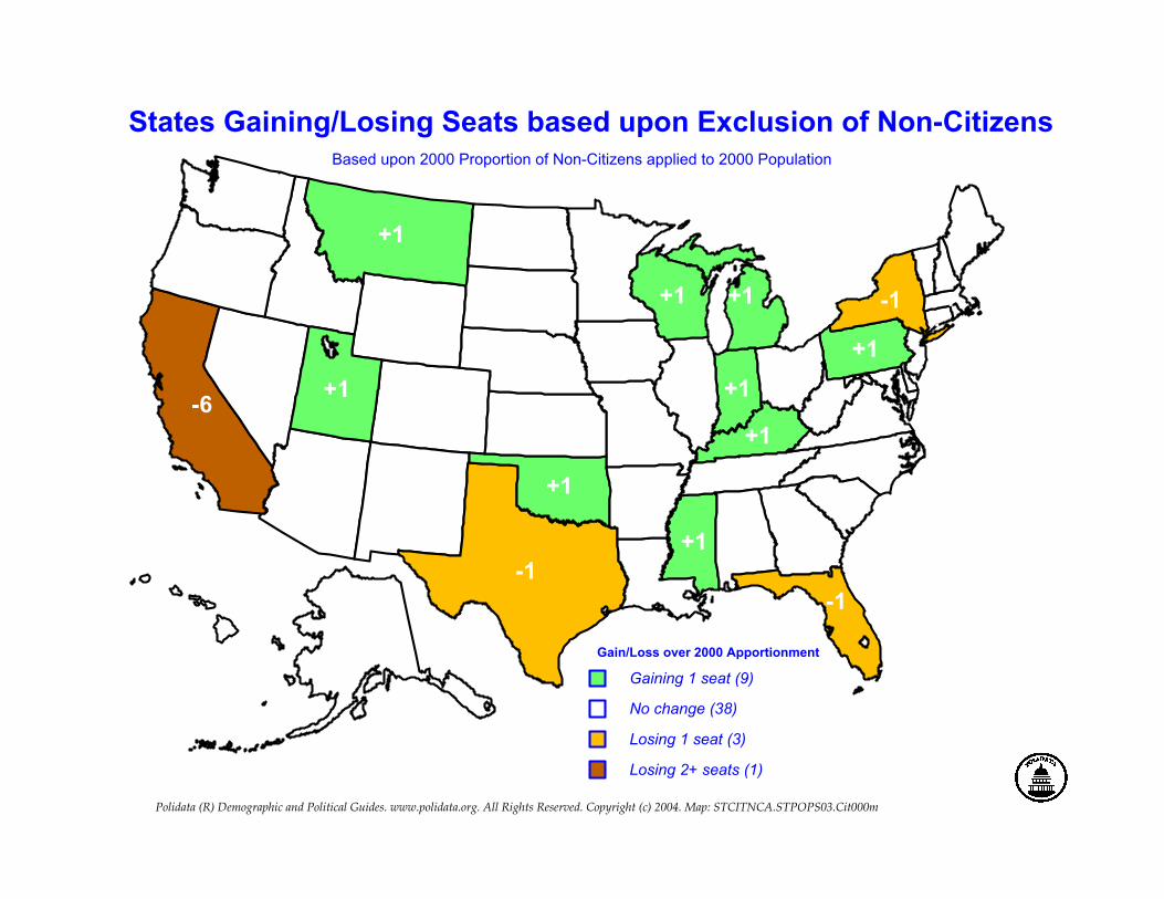
Florida is heavier, at 1.56 members per million persons, than that of a person in Texas at 1.53 members per million persons5 with respect to their representation in the House. Factoring in the differential in the voting age proportion for these two states produces a different result. With an estimated 494,972 persons of voting age in a Florida district (641,156 x 77.2%) and 469,033 persons of voting age in a Texas district (653,250 x 71.8%), the representational weight of the person in Florida, at 2.02 members per million persons of voting age, is now less than the weight of the person in Texas, at 2.13 members per million persons of voting age6. The second difference between inhabitants and voters is not so obvious. This difference is citizenship. The census has collected this information from respondents for the past few censuses, though it is now only a sample question. Nevertheless, it suffices for our purpose here, which is to point out the degree to which disparities exist in the apportionment process. For 2000, the states of California and Florida had approximately equal populations per member of the U.S. House. Yet, California, at 15.9%, had the highest percentage of any state that is non-citizen. Florida, at 9.2%, was ranked sixth amongst the states. Given California’s persons per member of 640,204, there are an estimated 538,412 citizens per member. With Florida’s 641,156 persons per member, there are an estimated 582,170 citizens per member. Thus the representational weight of person in California, at 1.85 members per million citizens, is heavier than that of a person in Florida, at 1.72 members per million citizens7. Apportionment and the Electoral College: Just as persons below the voting age can not vote, so too, non-citizens are deprived of this privilege. However, the young, the non-citizen, and the unregistered potential voter are still represented in the House. Moreover, while they can not make a personal choice in the election, they do “vote” for President, albeit indirectly. All three of these groups are factored into the apportionment, which is the basis for the Electoral College. States receive seats based upon the presence of the young, the non-citizen or the unregistered and not for voters or eligible voters. They have a vote in the Presidential Election as their state may have received electoral votes based upon their presence. For example, using the estimates of non-citizens from the 2000 census, we can run the apportionment formula and estimate the impact. A comparison of the apportionment determined from the 2000 census with that excluding non-citizens would result in a shift of 9 seats amongst 13 states. California would clearly be the largest loser: 6 seats could be lost dropping the delegation from 53 to 47 members. The other states that could lose by the exclusion of non-citizens are Florida, New York and Texas at 1 each.

5 For FL: 1/641,156. For TX: 1,653,250. 6 For FL: 1/494,972. For TX: 1/469,033. 7 For CA: 1/538,412. For FL: 1/582,170.

Apportionment and Fair Representation, Mar 2004, page 4

The states that could gain a seat by the exclusion of non-citizens include 4 states in the East and Midwest, regions that have been losing representation for the past generation. The states that could gain include Pennsylvania, Indiana, Michigan, and Wisconsin as well as Kentucky, Mississippi, Oklahoma, Montana and Utah. The impact that such an apportionment could have had on the 2000 Presidential Election would have been significant. The results of the 2000 election, one of the closest in our nation’s history, ended up in the Electoral College as 271 votes for Bush and 267 votes for Gore8, a Bush margin of 4 votes. But, the 2000 election was held under the 1990 Apportionment. Applying the 2000 Apportionment would increase the Bush margin, making the count 278 Bush to 260 Gore, a shift of 7 votes, and a Bush margin of 18 votes. Applying the 2000 Apportionment but excluding non-citizens, the count would be 282 Bush to 256 Gore, a shift of 4 votes, and a Bush margin of 26 votes. Districting and Votes Cast: Another perspective for the review of the role of apportionment9 is to consider the differential turnout of votes cast in congressional districts. The best data to use for this purpose are the results of the 2000 Presidential Election by Congressional District. Using the results for the Presidential Election helps to minimize the impact of factors that are specific to the Congressional Elections. Voter turnout for President in any district should not be significantly affected by factors affecting the congressional race. In this case, using the results for the 2000 election also coincides with the census data very well with a minimum of difference due to time. However, in all but a handful of states, there is no official compilation of these results. They must be compiled, district-by-district, from precinct-level election results. This requires contact with hundreds of local election officials. Even then, many problems remain, notably split precincts and centrally counted absentee or early votes. There is some judgment required depending upon the status of the data and the political geography. Polidata has played a role in the compilation of these data for the past 5 elections, in conjunction with several national organizations, including the Republican National Committee, Congressional Quarterly, the National Journal and the Cook Political Report. If the At-Large states are once again excluded from this dataset, it is clear that the difference in turnout of actual voters varies greatly across the nation. To some extent this is a factor of the disparities due to state boundaries. However, by reviewing districts in one state only, this problem is eliminated and the differences are still evident. For example, consider the 52 districts in California for the 2000 election.

8 Actually there was one faithless elector in D.C. who did not vote for Gore but we will assume this would, under normal circumstances, be a vote for the Democrat nominee. 9 While there may be a technical distinction between apportionment and districting, the term is used here to refer to the entire multi-step process of apportioning political power. This is the inclusive manner by which courts generally use the term to designate the overall process. Except for theAt-Large states, apportionment without districting is an incomplete process.

Apportionment and Fair Representation, Mar 2004, page 5

The California district that evidenced the highest turnout in the 2000 Presidential Election was CD-4 (Doolittle-R), with 326,224 votes cast for President. The California district with the lowest turnout was CD-33 (Roybal-Allard-D), with 76,762 votes. There were 10,965,856 total votes cast in the state for the Presidential Election, an average of 210,882 for each of the then 52 districts. The overall range here was 249,462 votes, or a staggering 118% of the average (ideal) votes per district. If we broaden the review to the 5 districts in California with the highest turnout in the Presidential Election versus the 5 districts in California with the lowest turnout, we find that there is still a huge disparity. The average for the highest turnout districts was 301,462 votes; the average for the lowest turnout districts was 109,052 votes. This represents an overall range of 192,410 or 91% of the ideal. Using these averages, the electoral weight of a voter in one of the districts with the high turnout, at 3.32 members per million voters, is significantly less than that of a voter in one of the districts with the low turnouts, at 9.17 members per million voters10. If we review districts across the country, a similar pattern emerges. The average for the 16 districts with a Presidential turnout over 325,000 was 344,361 votes. The average for the 18 districts with a Presidential turnout under 150,000 was 126,204 votes. This translates into an electoral weight for a voter in the high turnout districts, at 2.90 members per million voters, which is substantially lower than the electoral weight of a voter in the low turnout districts, at 7.92 members per million voters11. Districting and Common Characteristics: There are two commonalities in these high versus low turnout districts: political affiliation and race and ethnicity. We will review the top and bottom 44 districts as this represents 10% of the total of 435. Of the 44 districts with the highest turnout in the Presidential race, 26 voted for Bush, 18 for Gore. Similarly, 29 of these elected a Republican to the 107th Congress, 15 elected a Democrat. The average margin of victory (in the Presidential race) in these districts was 19.7%. Of the 44 districts with the lowest turnout in the Presidential race, 2 voted for Bush, 42 voted for Gore. Similarly, only 2 elected Republicans to the House, 42 elected Democrats. The average margin of victory (in the Presidential race) was 45.9%, Thus, from the partisan perspective, there is clearly a one-sided advantage for the Democrats. They have many districts, the so-called “cheap seats”, in which they are able to win seats with few votes cast, with little competition and with a heavier electoral weight. Of the 44 districts with the highest turnout, none of them had a significant subgroup of any racial or ethnic minority except one which had a group of Native Americans (AZ-6).

10 For the high turnout districts: 1/301,462. For the low turnout districts: 1/109,052. 11 For the high turnout districts: 1/344,361. For the low turnout districts: 1/126,204.

Apportionment and Fair Representation, Mar 2004, page 6

Of the 44 districts with the lowest turnout, all but 2 of them (TX-13 and TX-24) were classified as having a significant group presence of either Black/African American, or Hispanic/Latino or Asian. Thus, minority groups have an advantage in that many of their seats are low turnout districts with little competition and a heavier electoral weight. It is clear that there is a large degree of disparity between the electoral weights of some residents, or voters, in the nation compared with those of others in other districts. Districting and Population Equality: The concern with population equality is not that equipopulous districting minimizes all redistricting evils but that it is a commonly accepted means of attempting to level the playing field in an objective fashion12. While there is some debate about whether apportionment is a matter of representation or electoral equality, it is clear the genesis of the apportionment law has been a focus on electoral equality. Equal population was seen merely as a means of equalizing voting strength. That is, that the goal of apportionment is still to minimize the inequality in voting strength so that “one man's vote in a congressional election is to be worth as much as another's.” See Wesberry v. Sanders, 376 U.S. 1 (1964), (emphasis added).

Weighting the votes of citizens differently, by any method or means, merely because of where they happen to reside, hardly seems justifiable. One must be ever aware that the Constitution forbids “sophisticated as well as simple-minded modes of discrimination." Lane v. Wilson, 307 U.S. 268, 275 ; Gomillion v. Lightfoot, 364 U.S. 339, 342 . Reynolds v. Sims, 377 U.S. 533 (1964).

While there is still some difference of opinion as to how close a state legislature needs to come towards perfect equality in any reapportionment plan, it is clear that the fundamental goal should still be reaching 0% whenever practicable. The opinion in the recent apportionment case from Georgia13 (Larios v. Cox, N.D., GA, 2004), summarizes the one-person, one-vote reapportionment law as it has been shaped by a generation of court review. Contrary to some reports in the press14 this case was merely a logical reapplication of apportionment law that had been on the books since the Reapportionment Revolution of the 1960s. While Reynolds v. Sims, 377 U.S. 533 (1964) was the seminal case dealing with state legislative districting, another case decided the same day, Roman v. Sincock, 377 U.S. 695 (1964) addressed the issue of what was forbidden in the drawing of district boundaries. The courts were to determine if the state

12 In fact, a few states made a narrow range part of their adopted criteria to minimize the ability for redistricting shenanigans. (E.G., South Carolina at +/- 1% or Virginia at +/- 2%.) In other states, the legislative plans were drawn with a 0% overall deviation. (E.G., California or Illinois.) 13 For the sake of disclosure, Polidata principal consultant Clark Bensen was one of the expert witnesses for the plaintiffs. 14 N.B., the editorial in the New York Times for February 23, 2004 which misclassifies the case as one of partisan gerrymandering. In actuality, the partisan gerrymandering claim was dismissed by the court. The case was clearly based upon the one-person, one-vote jurisprudence.

Apportionment and Fair Representation, Mar 2004, page 7

process showed that “there has been a faithful adherence to a plan of population-based representation, with such minor deviations only as may occur in recognizing certain factors that are free from any taint of arbitrariness or discrimination.” The process of the Georgia legislative lines was most clearly not one that represented the neutral application of legitimate state interests. The state admittedly underweighted districts that were in areas that were already underweighted due to population loss. On the other end of the scale, they overpopulated districts that had experienced the largest growth over the past two decades. The overwhelming proportion of the underweighted districts leaned Democrat and the overwhelming proportion of the overweighted districts leaned Republican. The state plan was an attempt to contain the votes of the high growth areas (Republicans) and install a hold-harmless cushion for the areas that had been experiencing population loss for several decades (Democrats). Moreover, there was a clear discrimination against Republican incumbents (nearly half of the Republican caucuses were paired in the plans whereas almost no Democrats were paired). The plan also discriminated against residents who lived in areas supporting Republicans in general and against residents who lived in areas that had experienced continued high growth. Moreover, the impact was not inconsequential. Over 40% of the districts in the House plan had a population deviation over 4% and nearly 67% of the districts in the Senate plan were at the same level. There were hardly any districts at all near the 0%. The court found that these activities supported the conclusion that the “favoritism built into the Georgia House and Senate Plans created more than a taint of abritrariness and discrimination, violating Equal Protection by diluting the votes of citizens” in one area of the state and overweighting those in another. The Georgia case reaffirmed that the so-called “10% rule15” is only a rebuttable presumption and not a “safe-harbor” wherein anything goes. Clearly, the Georgia case points out that states can not use this 10% “window” to discriminate or to be arbitrary in the drafting of an apportionment plan. Equal Population and the Historic Record: A brief review of some selected states over time illustrates that the notion of population equality has had a checkered past in the American experiment in democracy. For much of the period before the Reapportionment Revolution of the 1960s, most districts were created solely upon the lines of political subdivision boundaries, e.g., counties, towns and cities, or wards within

15 That is, that range of the maximum positive deviation from the ideal to the maximum negative deviation would be under 10%. This could be -4.5% to +5.5% but in practice it is almost always from -5% to +5%.

Apportionment and Fair Representation, Mar 2004, page 8

cities. This had its own set of problems, some of which culminated in the abolishment of the so-called “county-unit” system in Georgia16. As one can imagine, this made the degree to which equal population was the standard amongst districts somewhat of a random event. Using these large units of geography and without the benefit of computers, there was bound to be some substantial variance even if a good faith effort was made to equalize population. Some states did manage to draw district lines within reasonable limits of overall deviation for their congressional districts. For example, West Virginia following the 1900 census had an overall range of only 5.5% while New York had an overall range of 57.8%. Following the 1930 census, Minnesota created a plan with an overall range of 17.4% while New York had an overall range of 245.1%. The state of Georgia has had a particularly high overall range in several plans, largely due to the containment of the Atlanta area counties into one district. Following the 1930 census, the range in Georgia was 67.3%; following the 1940 census the range was 80.7%; following the 1950 census the range was 134.3%; following the 1960 census the range was 139.9%. In each of these apportionment plans, it was CD-5 (basically Fulton, DeKalb and Rockdale counties) that had the highest number of persons assigned to it. For example, for the plan first drawn using the 1960 census data, the district with the smallest number of persons was CD-9 with 272,154 persons; CD-5 was assigned 823,680 persons17. Conclusion: Over forty years have passed since the Reapportionment Revolution began with Baker v. Carr, 369 U.S. 186 (1962). Four reapportionment cycles have been completed since the first flurry of activity in the mid-1960s. Over the passage of time most apportionment stakeholders have become accustomed to think of equipopulous districting as the great equalizer and as a concern that no longer needs to be addressed. Yet, as we have seen in the examples above, a great deal of inequality still exists in the process of apportionment and districting. From both Wesberry18 and Reynolds19 it is clear that the notion of population equality is only a means by which electoral equality can be attained. As we continue to refine the law of apportionment and as political activists call for reform of some of our fundamental electoral systems, this seems to be an important consideration to bear in mind. 16 The county-unit system involved statewide elections and overweighted the role of the small rural counties in determining the winner. See Gray v. Sanders, 372 U.S. 368 (1963), 17 In fact, it was this very situation that resulted in Wesberry v. Sanders, 376 U.S. 1(1964), the case that established that the Art. I, sec. 2, “means that as nearly as is practicable one person's vote in a congressional election is to be worth as much as another's.” 18 Ibid. 19 “Since the achieving of fair and effective representation for all citizens is concededly the basic aim of legislative apportionment” Reynolds v. Sims, 377 U.S. 533, 566 (1964),

Apportionment and Fair Representation, Mar 2004, page 9

Enclosures: 1. Map: States Gaining/Losing Seats based upon Exclusions of Non-Citizens 2. Press Release: Possible Delegation Changes in the U.S. House for 2012

[I:\polidata\COMMENTS\dc05_census\sympos1a.doc]

..

.

..

-6.

.

-1

+1

.

.

.

+1

.

.+1

..

.

..

+1

+1

+1

.

..

.

..

-1

.

..

.+1

..

+1+1 -1

..

..

.

.

.

.

Gain/Loss over 2000 Apportionment

Gaining 1 seat (9)

No change (38)

Losing 1 seat (3)

Losing 2+ seats (1)

States Gaining/Losing Seats based upon Exclusion of Non-CitizensBased upon 2000 Proportion of Non-Citizens applied to 2000 Population

Polidata (R) Demographic and Political Guides. www.polidata.org. All Rights Reserved. Copyright (c) 2004. Map: STCITNCA.STPOPS03.Cit000m

PRESS RELEASE

POSSIBLE DELEGATION CHANGES IN THE U.S.HOUSE FOR 2012 Population Trends for the 2010 Apportionment; the 2003 Estimates

February 19, 2004 CLARK BENSEN1

POLIDATA ® Political Data Analysis

For political observers, it’s never too early to monitor the possibilities of how population shifts over the decade may affect the political landscape following the next census. For politicians seeking higher office, thinking years in advance for the upcoming election calendars, this annual exercise is a must for any potential bid. For those like me, who have been steadily involved in the political thicket of apportionment and districting following the most recent census, well, some things get set aside for a while2. Nevertheless, here we have another installment in the periodic prognostication of how seats will shift amongst the states for the 2012 election. The Bureau of the Census releases estimates of the population by state annually. However, the Bureau does not generally release state-level projections of the population on a regular basis. These annual estimates form the basis for these numbers which are projected out to 2010 by POLIDATA. Projection: There are several means of projection, some more sophisticated than others. For the sake of these projections, based upon estimates very early in the decade, an unsophisticated methodology is used. The growth rates for each state for the previous two years, here from 2001-2002 and from 2002-2003, are averaged. This rate is then applied to the 2003 estimate in a step-wise fashion through 2010. The apportionment formula is then run on the basis of these 2010 projections.

1 Clark H. Bensen, B.A., J.D., consulting data analyst and attorney doing business as POLIDATA ® Polidata Data Analysis and a publisher of data volumes operating as POLIDATA ® Demographic and Political Guides. POLIDATA is a demographic and political research firm located outside Washington, D.C. 2 The results normally are released in December but we were preparing for the Georgia apportionment trial that commenced the first week of January 2004.

POLIDATA® Political Data Analysis DATABASE DEVELOPMENT, ANALYSIS AND PUBLICATION;

POLITICAL AND CENSUS DATA; LITIGATION SUPPORT

CLARK BENSEN POLIDATA· 3112 Cave Court, Suite B· Lake Ridge, VA 22192-1167

Tel: 703-690-4066 · Fax: 202-318-0793 (efax)· email: clark@polidata.org PUBLISHER OF THE POLIDATA ® DEMOGRAPHIC AND POLITICAL GUIDES AND ATLASES

website: www.polidata.org

Population Trends for the 2010 U.S. House Apportionment, the 2003 Estimates, page 2

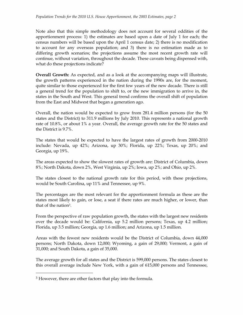
Note also that this simple methodology does not account for several oddities of the apportionment process: 1) the estimates are based upon a date of July 1 for each; the census numbers will be based upon the April 1 census date; 2) there is no modification to account for any overseas population; and 3) there is no estimation made as to differing growth scenarios; the projections assume the most recent growth rate will continue, without variation, throughout the decade. These caveats being dispensed with, what do these projections indicate? Overall Growth: As expected, and as a look at the accompanying maps will illustrate, the growth patterns experienced in the nation during the 1990s are, for the moment, quite similar to those experienced for the first few years of the new decade. There is still a general trend for the population to shift to, or the new immigration to arrive in, the states in the South and West. This general trend confirms the overall shift of population from the East and Midwest that began a generation ago. Overall, the nation would be expected to grow from 281.4 million persons (for the 50 states and the District) to 311.9 millions by July 2010. This represents a national growth rate of 10.8%, or about 1% a year. Overall, the average growth rate for the 50 states and the District is 9.7%. The states that would be expected to have the largest rates of growth from 2000-2010 include: Nevada, up 42%; Arizona, up 30%; Florida, up 22%; Texas, up 20%; and Georgia, up 19%. The areas expected to show the slowest rates of growth are: District of Columbia, down 8%; North Dakota, down 2%, West Virginia, up 2%; Iowa, up 2%; and Ohio, up 2%. The states closest to the national growth rate for this period, with these projections, would be South Carolina, up 11% and Tennessee, up 9%. The percentages are the most relevant for the apportionment formula as these are the states most likely to gain, or lose, a seat if there rates are much higher, or lower, than that of the nation3. From the perspective of raw population growth, the states with the largest new residents over the decade would be: California, up 5.2 million persons; Texas, up 4.2 million; Florida, up 3.5 million; Georgia, up 1.6 million; and Arizona, up 1.5 million. Areas with the fewest new residents would be the District of Columbia, down 44,000 persons; North Dakota, down 12,000; Wyoming, a gain of 29,000; Vermont, a gain of 31,000; and South Dakota, a gain of 35,000. The average growth for all states and the District is 599,000 persons. The states closest to this overall average include New York, with a gain of 615,000 persons and Tennessee,

3 However, there are other factors that play into the formula.

Population Trends for the 2010 U.S. House Apportionment, the 2003 Estimates, page 3

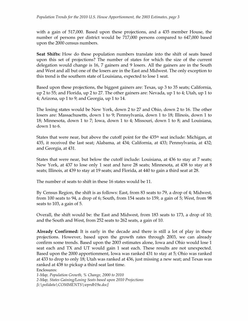
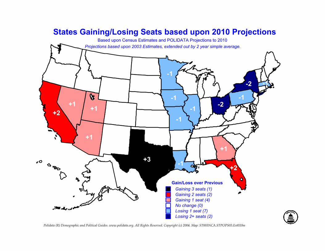
with a gain of 517,000. Based upon these projections, and a 435 member House, the number of persons per district would be 717,000 persons compared to 647,000 based upon the 2000 census numbers. Seat Shifts: How do these population numbers translate into the shift of seats based upon this set of projections? The number of states for which the size of the current delegation would change is 16, 7 gainers and 9 losers. All the gainers are in the South and West and all but one of the losers are in the East and Midwest. The only exception to this trend is the southern state of Louisiana, expected to lose 1 seat. Based upon these projections, the biggest gainers are: Texas, up 3 to 35 seats; California, up 2 to 55; and Florida, up 2 to 27. The other gainers are: Nevada, up 1 to 4; Utah, up 1 to 4; Arizona, up 1 to 9; and Georgia, up 1 to 14. The losing states would be New York, down 2 to 27 and Ohio, down 2 to 16. The other losers are: Massachusetts, down 1 to 9; Pennsylvania, down 1 to 18; Illinois, down 1 to 18; Minnesota, down 1 to 7; Iowa, down 1 to 4; Missouri, down 1 to 8; and Louisiana, down 1 to 6. States that were near, but above the cutoff point for the 435th seat include: Michigan, at 435, it received the last seat; Alabama, at 434; California, at 433; Pennsylvania, at 432; and Georgia, at 431. States that were near, but below the cutoff include: Louisiana, at 436 to stay at 7 seats; New York, at 437 to lose only 1 seat and have 28 seats; Minnesota, at 438 to stay at 8 seats; Illinois, at 439 to stay at 19 seats; and Florida, at 440 to gain a third seat at 28. The number of seats to shift in these 16 states would be 11. By Census Region, the shift is as follows: East, from 83 seats to 79, a drop of 4; Midwest, from 100 seats to 94, a drop of 6; South, from 154 seats to 159, a gain of 5; West, from 98 seats to 103, a gain of 5. Overall, the shift would be: the East and Midwest, from 183 seats to 173, a drop of 10; and the South and West, from 252 seats to 262 seats, a gain of 10. Already Confirmed: It is early in the decade and there is still a lot of play in these projections. However, based upon the growth rates through 2003, we can already confirm some trends. Based upon the 2003 estimates alone, Iowa and Ohio would lose 1 seat each and TX and UT would gain 1 seat each. These results are not unexpected. Based upon the 2000 apportionment, Iowa was ranked 431 to stay at 5; Ohio was ranked at 433 to drop to only 18; Utah was ranked at 436, just missing a new seat; and Texas was ranked at 438 to pickup a third seat last time. Enclosures: 1-Map, Population Growth, % Change, 2000 to 2010 2-Map, States Gaining/Losing Seats based upon 2010 Projections [i:\polidata\COMMENTS\wprdb19a.doc]

-1

+1

+2+1

+3

+1-1

-1

-1

-1

+1

+2

-1-2

-2 -1

Gain/Loss over Previous Gaining 3 seats (1) Gaining 2 seats (2) Gaining 1 seat (4) No change (0) Losing 1 seat (7) Losing 2+ seats (2)

States Gaining/Losing Seats based upon 2010 ProjectionsBased upon Census Estimates and POLIDATA Projections to 2010

Projections based upon 2003 Estimates, extended out by 2 year simple average.

Polidata (R) Demographic and Political Guides. www.polidata.org. All Rights Reserved. Copyright (c) 2004. Map: ST003NCA.STPOPS03.Est010m