Page 1
POLITECNICO DI MILANO
Facoltà di Ingegneria dei Sistemi
Corso di Laurea Specialistica in Ingegneria Gestionale
A MODEL OF TOTAL LANDED COST FOR
GLOBAL SUPPLY CHAIN MANAGEMENT
Relatore: Ing. Marco Melacini
Correlatore: Prof. Eero Eloranta
Tesi di Laurea di:
Simone Bonanni 736553
Anno Accademico 2010-2011
Page 3
ii
Acknowledgments
I wish to thank my Italian and Finnish supervisors Professor Marco Melacini and
Professor Eero Eloranta for guiding me during the realization of this research as well
as for their inspiring suggestions. I would like to thank my company instructor Panu
Kaila for involving me in this project and for the fruitful discussions that we had in
the past months. In general, thanks to the Globenet project researchers, with their
suggestions they contribute to the development of this research. Then, I would like to
express my gratitude to the people working in the case firm that contributed actively
for the realization of this work.
I would like to thank Finland and the Finnish people for the great opportunities
given to me. Among the Finnish friends, Petri, Tommi and Sanna deserve special
thanks.
I wish to thank also my Italian friends. They have been a necessary guidance in
the last 5 years of my life. Thanks to Chine and Rosi, they have taught me how to
love the reality. Thanks to Rosso, he has spiced up my life. Thanks to Pas, he has
never given up on me. Thanks to Peppe, he has made of me a better person. Thanks
to Paolo, Stefano, Seba, Zana, Funch and Anna, they have been great companions in
the recent years. The “Gruppo gestio” formed by Dave, Bibo, Stefy, Fede and Dany
also deserves many thanks. Finally, the friends met in “Totti” and “Interfacoltà” has
contributed greatly for my growth as a man. Among them I would like to mention
Simo Lena, Jack, Charlie, Bobo, Peco, Dory, Danielao, Luca, Dome, Ggg, Tommy
and Macca.
In the last three years, I met a bunch of great people from all around the world.
Even though it is impossible to list all of them, my appreciations go to them as well.
Special thanks go to Yiwen, Alberto, Goncalo, Juli, Emre, Yusuke, Jessica and Sum
for their passion for life. Their friendship has been a necessary part of my life.
My family has been a great support during my time in Finland and during all my
life. So my thanks go to my father (Fabio), my “mamma” (Antonella), my
grandmother (Elena), my brothers (Daniele and Matteo) and my sister-in-law
(Melania).
Simone Bonanni
Page 4
iii
Abstract
The recent economic trends has pushed companies to move their operations
globally. One of the key decisions concerns the allocation of the final demand
according to the available production facilities. To support this decision, the
estimation of the total landed cost is suggested. The studies identified in literature
limit their scopes in terms of products/markets and costs considered, while a wide
perspective on the costs should be considered to reach a satisfactory solution. The
purpose of the study is to build a comprehensive total landed cost model for the
estimation of the costs related to tactical configurations (i.e. scenario analysis) in a
case study
The research takes a constructive approach (Kasanen et al., 1993). Starting from
the needs expressed by the managers of a case study, it aims to build a tool to answer
to these needs and contribute to the literature on the topic. For the scope of the
research, fourteen people throughout the organization were actively involved in the
process for the collection of qualitative and quantitative data.
As result of the study, a model of the total landed cost for tactical planning is
provided to the company. The model evaluates the effects of production allocation
decisions on the following costs: transportation (inbound and outbound), customs,
handling, inventory carrying costs, hidden costs and production costs. Its internal
validity was tested and discussed with the future users of the application. As a result,
it is shown that considering the total landed cost improves management’s
understanding of the profitability and robustness of their decisions. The validity and
the limits of the approach are discussed. Finally, the study identifies new areas for
future research.
Page 5
iv
Table of contents
ABSTRACT ........................................................................................................ III
SOMMARIO .......................................................................................................... 1
CHAPTER 1 ........................................................................................................... 5
1. INTRODUCTION .......................................................................................... 5
1.1 BACKGROUND ........................................................................................... 5
1.2 RESEARCH PROBLEM ................................................................................. 5
1.3 GOALS OF THE RESEARCH .......................................................................... 7
1.4 METHODS .................................................................................................. 7
1.5 STRUCTURE OF THE STUDY ...................................................................... 10
CHAPTER 2 ......................................................................................................... 11
2. GLOBAL SUPPLY CHAIN MANAGEMENT ......................................... 11
2.1 GLOBALIZATION TREND .......................................................................... 12
2.2 SUPPLY CHAIN STRATEGY ........................................................................ 13
2.3 STRATEGIC, TACTICAL AND OPERATIONAL LEVEL DECISIONS .................. 14
2.4 SUPPLY CHAIN PLANNING ........................................................................ 15
2.5 LITERATURE GAP ANALYSIS .................................................................... 19
2.6 MODELING THE TOTAL LANDED COST ...................................................... 21
2.6.1 Production costs ............................................................................. 22
2.6.2 Logistics costs ................................................................................. 22
2.6.3 Hidden costs ................................................................................... 26
2.7 SUPPLY CHAIN COSTING .......................................................................... 26
2.7.1 Activity based costing ..................................................................... 26
2.7.2 Supply chain costing for planning support ..................................... 28
Page 6
v
CHAPTER 3 ......................................................................................................... 30
3. CASE DESCRIPTION ................................................................................. 30
3.1 OVERVIEW OF THE MARKET ..................................................................... 30
3.2 SUPPLY CHAIN CONFIGURATION .............................................................. 31
3.2.1 Description of the production processes ........................................ 35
3.3 STRUCTURE OF THE COSTS ....................................................................... 37
CHAPTER 4 ......................................................................................................... 38
4. TOTAL LANDED COST MODEL ............................................................ 38
4.1 SET THE PROBLEM ................................................................................... 38
4.1.1 Planning horizon ............................................................................ 38
4.1.2 Model characteristics ..................................................................... 39
4.1.3 The scope of the model ................................................................... 40
4.2 MAP OF THE COSTS .................................................................................. 42
4.2.1 Inbound logistics costs ................................................................... 45
4.2.2 Outbound logistics costs ................................................................. 46
4.2.3 Hidden costs ................................................................................... 50
4.3 COST DRIVERS ......................................................................................... 50
4.4 MODEL FORMULATION ............................................................................ 54
4.4.1 Inbound logistics ............................................................................ 55
4.4.2 Outbound logistics .......................................................................... 61
4.4.3 Total landed cost ............................................................................ 75
4.5 VALIDATE THE MODEL ............................................................................ 75
4.5.1 Accuracy ......................................................................................... 76
Page 7
vi
CHAPTER 5 ......................................................................................................... 81
5. RESULTS AND DISCUSSION ................................................................... 81
5.1 UNDERSTANDING CUSTOMER PROFITABILITY .......................................... 81
5.2 SCENARIO ANALYSIS ............................................................................... 82
5.3 THEORETICAL CONTRIBUTION ................................................................. 88
5.4 CONTRIBUTION TO SUPPLY CHAIN COSTING LITERATURE ........................ 88
5.5 EXTERNAL VALIDITY OF THE STUDY ........................................................ 90
5.6 LIMITS OF THE SOLUTION......................................................................... 92
CHAPTER 6 ......................................................................................................... 94
6. CONCLUSIONS ........................................................................................... 94
6.1. KEY FINDINGS ......................................................................................... 94
6.2. FUTURE RESEARCH .................................................................................. 97
REFERENCES .................................................................................................... 98
APPENDIX ......................................................................................................... 103
APPENDIX 1 ...................................................................................................... 103
Page 8
vii
List of Figures
FIGURE 1-1 - CONSTRUCTIVE APPROACH (KASANEN ET AL., 1993) ............................... 8
FIGURE 2-1 – SCOPES OF THE MODEL .......................................................................... 19
FIGURE 2-2 - PLANNING HORIZONS AND CHARACTERISTICS OF THE MODELS ............... 20
FIGURE 3-1 - SUPPLY CHAIN MAP ................................................................................ 32
FIGURE 3-2 – CONTRACT TERMS WITH SUPPLIERS ....................................................... 35
FIGURE 3-3 - ALPHA MANUFACTURING PROCESS ......................................................... 37
FIGURE 3-4 - COMPOSITION OF THE TOTAL LANDED COST [FISCAL YEAR 2009] .......... 37
FIGURE 4-1 – MAP OF THE COSTS ................................................................................ 43
FIGURE 4-2 – HISTORICAL DATA ON LOGISTICS COSTS ................................................ 43
FIGURE 4-3 – PROCESSES AT THE LOCAL DEPOSITS ...................................................... 49
FIGURE 4-4 - COMPARISON REAL DATA AND MODEL ................................................... 78
FIGURE 5-1 – RELEVANCE OF THE LOGISTICS COSTS FOR A SELECTION OF PRODUCTS . 82
FIGURE 5-2 – PRODUCTION MOVED TO CHINA ............................................................. 85
FIGURE 5-3 - PRODUCTION MADE LOCALLY................................................................. 86
FIGURE 5-4 - NEAR-SHORING FOR FLEXIBILITY ........................................................... 86
Page 9
viii
List of Tables
TABLE 2.1 LITERATURE REVIEW ON TACTICAL PLANNING MODELS ............................. 18
TABLE 4.1 – CLASSIFICATION OF THE MODEL .............................................................. 42
TABLE 4.2 – MATRIX COSTS AND DRIVERS .................................................................. 51
TABLE 4.3 - DECISION PARAMETERS ........................................................................... 52
TABLE 4.4 – THE INFLUENCE OF DECISIONS PARAMETERS ON LOGISTICS COSTS .......... 53
TABLE 4.5 - PARTIALLY INDEPENDENT PARAMETERS .................................................. 53
TABLE 4.6 - EXTERNAL PARAMETERS .......................................................................... 54
TABLE 5.1 TOTAL LANDED COST (TLC) FOR THREE PRODUCTION ALLOCATION
CONFIGURATIONS, COSTS EXPRESSED IN MILLION OF € ........................................ 87
TABLE 6.1 - COST DRIVERS CATEGORIZATION ............................................................. 96
Page 10
1
Sommario
Negli ultimi tre decenni, i trend economici hanno spinto le aziende a globalizzare
la supply chain attraverso la delocalizzazione della produzione e lo spostamento della
base fornitori verso il Far East. Negli ultimi anni, l’aumento dei costi del petrolio,
l’apprezzamento della moneta Cinese e l’inflazione del costo dei fattori produttivi nei
paesi in via di sviluppo sta portando alla revisione delle scelte di offshoring. In
questo contesto, la disciplina di global supply chain management risulta avere un
ruolo sempre più importante nel determinare i risultati delle aziende. I manager
devono prendere decisioni a tre livelli diversi: strategico, tattico e operativo. Una
delle scelte chiave che i manager devono affrontare a livello tattico è l’allocazione
della domanda finale ai siti produttivi disponibili. Per valutare queste scelte,
accademici e professionisti suggeriscono l’utilizzo di modelli di Total Landed Cost.
Gli studi identificati nella letteratura limitano il loro ambito in termini di mercati/
prodotti e costi considerati. L’obiettivo di questo studio è quindi lo sviluppo di un
modello di total landed cost per la pianificazione tattica sulla base della stima dei
costi generati dall’intera supply chain per un case study.
Classificazione letteratura su allocazione della produzione
Partendo dalle necessità espresse dal management dell’azienda considerata
(chiamata Alpha in questo studio), lo scopo della ricerca è quello di fornire uno
Page 11
2
strumento per migliorare le decisioni di allocazione della produzione nel caso di
supply chain globale. Nell’ambito della ricerca, quattordici persone all’interno
dell’azienda sono state attivamente coinvolte per la raccolta di dati quantitativi e
qualitativi.
L’azienda considerata opera a livello global gestendo production plant in Estonia
e Cina e servendo clienti in Europa, Cina e USA. Il management dell’azienda
dispone di un modello per la valutazione dei costi di produzione. L’aumento
dell’incidenza dei costi logistici rende importante considerare anche tali costi per la
valutazione di decisioni di allocazione della produzione. Come risultato dello studio
è stato sviluppato per l’azienda in esame un software tool. Il modello dei costi
logistici proposto si basa sui principi dell’ Activity Based Costing e integra il
modello per la valutazione dei costi di produzione già in uso all’interno di Alpha.
Complessivamente, il modello permette di valutare le decisioni tattiche di
allocazione della produzione sulle seguenti voci di costo: trasporto (inbound e
outbound), costi doganali, movimentazione materiali, costi delle scorte (di ciclo, di
sicurezza e in transito), hidden costs (costi di qualità, fluttuazione dei tassi di cambio
e incremento del capitale circolante) e costi di produzione. Date le caratteristiche del
sistema produttivo di Alpha, l’orizzonte di pianificazione considerato è un anno.
L’assenza di effetti di stagionalità permette di utilizzare un time bucket di un anno.
Partendo dallo studio della struttura corrente della supply chain, i driver di costo
sono stati identificati e legati alle voci di costo considerate. Nella tabella di seguito è
mostrata la relazione esistente tra costi logistici e variabili decisionali:
Driver
direction Transportation Inventory Customs Handling
Shipment frequency
(Outbound) + + - + Not influenced
Production allocation Offshoring + + + + or -
Shipment frequency
(Inbound) + + - + Not influenced
Page 12
3
La validità del modello è stata discussa con i futuri utilizzatori dello strumento di
pianificazione. Il modello è testato sui dati storici e si stima un errore minore del
10%. Inoltre i dati generati dal modello rappresentano in modo appropriato la
struttura dei costi dell’azienda. Considerato l’ambito di applicazione, l’accuratezza
del modello è stata considerata adeguata da parte del management dell’azienda.
Per valutare i benefici legati alla stima del total landed cost, il modello è stato
applicato ai dati di previsione della domanda, contribuendo a migliorare la
comprensione del management sulla profittabilità dei prodotti. In particolare,
permette di identificare i prodotti per cui la decisione di allocazione della produzione
dovrebbe essere rivista.
Inoltre, il tool sviluppato permette di analizzare le decisioni tattiche sulla base di
diversi scenari. Le decisioni di allocazione della produzione possono essere valutate
al cambiare dei noli di trasporto, dei costi di mano d’opera, apprezzamento del RMB
etc.etc. L’applicazione del modello permette quindi una migliore comprensione delle
alternative a disposizione del management.
All’interno della ricerca, il modello valuta la decisione di allocazione della
produzione per 7 prodotti. L’analisi effettuata considera tre possibili scenari: (1)
offshoring della produzione, (2) produzione locale e (3) nearshoring di parte della
produzione per aumentare flessibilità della supply chain. Nello studio viene mostrato
come la valutazione del total landed cost permette di identificare alternative che
altrimenti non sarebbero considerate dal management (l’alternativa 3 dal punto di
vista dei costi di produzione non porterebbe a nessun vantaggio). Valutando la
variazione dei fattori di incertezza è possibile comprendere meglio anche la
robustezza della decisioni. Nel caso considerato l’apprezzamento dell’ RMB e
l’aumento dei costi di nolo aumenta fortemente i costi legati all’alternativa 2 (un
aumento fino al 30% dei costi totali).
I limiti del modello considerato sono evidenziati all’interno della tesi. Inoltre,
partendo da questo lavoro è possibile identificare possibili aree di ricerca futura.
Infatti, il gap identificato all’interno della letteratura risulta essere solo parzialmente
colmato. Come prossimo step potrebbe essere considerato lo sviluppo di un modello
di ottimizzazione delle decisioni tattiche. Inoltre, per una migliore stima degli effetti
Page 13
4
dell’incertezza sui costi totali, le variabili aleatorie dovrebbero essere modellate
come tali e non come variabili statiche.
Page 14
5
Chapter 1
1. Introduction
1.1 Background
This thesis is developed within a collaboration between Politecnico di Milano and
Aalto University, School of science and technology. This study is a part of a broad
research project named GlobeNet – Global operations network – run by the BIT
research center. The GlobeNet project aims to identify the success factors and the
designing rules in managing effectively global operations. It is sponsored by Tekes
and by 10 global companies. This study is made in close collaboration with one of
the ten companies, which in this study will be named “Alpha”. In relation to the
globalization of market economies, it is extremely important to understand the costs
involved in the processes from sourcing to product delivering. Indeed, a better
understanding of these expenses would allow the manager to get better information
on the products profitability. Furthermore, it would support the choices of the
managers on tactical planning.
1.2 Research problem
The recent economy trends pushed companies to move their operations globally
(Pontradolfo & Okogbaa, 1999; Zeng and Rossetti, 2003; Christopher et Al., 2006;
Bartlett et Al., 2008). The relocation of production facilities is increasing the
distances between production plants and markets (Pontradolfo & Okogbaa, 1999;
Zeng & Rossetti, 2003). Hence, the relevance of logistics costs in companies’
profitability is rising (Kruger, 2002). The research has focused mostly on strategic
decisions on supply chain design (Swaminathan & Tayur, 2004), while managing
companies operating in the global environment requires taking decisions also at the
tactical and operational levels (Schmidt & Wilhelm, 2000). To be successful in the
current environment, it is important for the companies to coordinate the operations of
their subsidiaries (Thomas & Griffin, 1996). One of the key decisions is about the
Page 15
6
allocation of the final demand according to the possible production facilities (Allon
& Van Mieghem, 2010). In this perspective, tactical decisions take a critical role in
determining companies’ performance.
Damme and Zon (1999) noticed that companies lack tools for tactical decision-
making based on logistics cost information. In many companies, the focus is rather
on manufacturing costs (Scully & Fawcett, 1993). However, the end-to-end costs
should be considered in order to understand the implications of decisions on the all
supply chain.
In the literature, there are very few works that propose techniques supporting
tactical planning based on cost modeling (Comelli et Al., 2008). A study made by
Erhun and Tayur (2003) shows the benefits of introducing the total landed cost as a
tool for influencing managerial decisions. As far as my literature review goes, their
research is one of the few studies that develops a total landed cost model for a real
case and evaluates the benefits of its application. The model proposed by the authors
is built to support the decisions at the operational level for an organization operating
in the retail industry. Therefore, its application to a company operating in another
environment for supporting tactical planning decisions would be of relevance for this
research area.
Alpha is a Finnish company operating in the power supply systems industry, the
global nature of its supply chain increases the complexities of decision-making.
Furthermore, the high competition that the company is facing makes cost efficiency a
requirement for enhancing profitability. For tactical planning purposes, the company
is currently using a “cost of goods sold” model. It is through the forecasts of final
demand and manufacturing expenses that the company’s managers take decisions on
production allocation. However, the model currently used does not give information
about the impact of tactical decisions on logistics costs. As highlighted by the
literature, the globalization of supply chain requires evaluating decisions on costs
generated by sourcing, manufacturing and delivering processes (Goel et al.,2008).
Therefore, Alpha’s managers are calling for a tool that would integrate the
information given by the “cost of goods sold” model to the information regarding
logistics costs.
Page 16
7
Hence, the research question that will guide the study is:
How should the total landed cost be modeled in order to support the tactical
decisions on how to run the operations in an efficient and effective way?
The focus of the model will be to provide a tool to support decision-making
mainly for production allocation problems.
1.3 Goals of the research
In agreement with the research question, the study aims to:
1. Identify the variables that affect the total landed cost for production and
delivering of products;
2. Develop a total landed cost model for the case study;
3. Assess the benefits of introducing a total landed cost model as a supportive
tool in the tactical planning processes of the case study.
In building the model, the focus is on balancing the need of information for
tactical decision-making with the costs of maintenance of the model itself. To limit
the complexity of the tool, some costs were excluded. For instance the customer
related costs, like shortage costs, are not considered.
1.4 Methods
In agreement with Kasanen et al. (1993), the research takes a constructive
approach and aims to solve a managerial problem and contribute to the knowledge on
the topic. In Figure 1-1, the elements characterizing the constructive approach are
shown.
Page 17
8
Figure 1-1 - Constructive approach (Kasanen et al., 1993)
Constructive research accepts subjectivity as a part of science. Studies following
this approach can be based on qualitative or quantitative data and they normally take
the form of case study (Kasanen et al., 1993). Hence in the work here reported, the
real needs of Alpha management are considered. The research aims to find an
innovative solution through the collection of qualitative and quantitative data.
The process for model development was structured in stages similar to the ones
proposed by Shapiro (2001) for the execution of supply chain studies: 1)“Organize
the study”; 2) “Collect the data”; 3) “Validate the data and model” and finally 4)
“Analyze scenarios”.
Organizing the study
The objective of the first stage was to define the decision-making situation in
which the model should support the managers. This led to decisions regarding the
basic characteristics of the model to be created. For this purpose the main users of
the model, e.g. the logistics managers and the executive vice president of the
operation, were interviewed.
Collecting the data
To balance the trade-off between accuracy and complexity of the model, it is
necessary to collect information regarding the case study (Billington & Davis, 1992).
Data regarding the current status of the supply chain and the characteristics of the
environment in which Alpha is operating were collected. The information was
collected through interviews (oral interviews and e-mails) with the employees
working in the various departments of the organization, as following:
Sales department (3 account managers and 1 customer support officer);
Page 18
9
Sourcing department (sourcing senior manager);
Logistics department (logistics manager and logistics supervisor);
Finance department (business controller and 3 accountants);
Information technology (2 information systems specialists);
Operations & sourcing (executive vice-president of the operations).
The aim of this stage was also to get an understanding of the information system
structure and of the currently available data. This is a crucial stage for ensuring the
accuracy of the model (Kosior & Strong, 2006) and limiting the need of new
measures.
Validating the data and model
Based on the information collected in the interviews and on the literature studied,
a descriptive model of the total landed cost of Alpha’s supply chain was built.
According to Shapiro (2001), a descriptive model aims to enhance the managers
understanding of supply chains. This type of model corresponds adequately to the
requirements expressed by Alpha managers. Indeed, they are looking for a model
that would improve their comprehension of the supply chain costs. However, the
model built does not propose algorithms for dynamic optimization.
For the development of the tactical planning model, five steps are proposed:
1. Setting the problem and defining the planning context of the decisions (i.e.
planning horizon and time buckets) to be evaluated.
2. Creating a map of the supply chain topology and identifying the most
significant costs.
3. Identifying the parameters that explain the costs and then classifying them in
decision parameters and “external” ones.
4. Defining the relations between input variables and the costs identified in step
2.
Page 19
10
5. Verifying the internal validity of the model through the evaluation of its
accuracy and practical usefulness, as well as through its application to real
cases.
Analyzing scenarios
The model was tested in order to demonstrate that the information given as output
matches the real behavior of the supply chain. In doing this, the historical data were
compared with the data generated by the model. Finally to show its usefulness,
different scenarios are analyzed and presented.
1.5 Structure of the study
In agreement with the constructive approach, the research process is constituted
by 6 stages (Kasanen et Al., 1993):
1. Finding a practical and significant problem which offers a research
opportunity;
2. Gaining an overall understanding of the topic;
3. Finding an innovative solution for the problem;
4. Demonstrating the internal validity of the solution identified;
5. Showing the theoretical connections and the contribution to the subject;
6. Discuss the applicability of the solution in other contexts.
The structure of the thesis is aligned with the 6 stages listed above. In the first
chapter the research problem and its relevance are presented. In the second and third
chapters, the overall knowledge (theoretical and practical) gained for the scope of the
study is presented through the literature review and the presentation of the basic
characteristics of the supply chain studied. In chapter 4, the model developed is
presented and validated. Finally in the 5th
and 6th
chapters, considerations about the
theoretical contribution of the work and the external applicability of the solution are
drawn. This structure shows the steps taken during the research in order to ensure
that each of the elements presented in Figure 1-1 were considered. This is
particularly important to ensure that a scientific approach of the problem is taken and
to avoid reducing the project to a consulting work (Kasanen et Al., 1993).
Page 20
11
Chapter 2
2. Global Supply Chain management
The globalization forces, the increasing importance of quality and time in
competition and the environmental uncertainties are just some of the trends that can
be considered responsible for the rising importance of supply chain management in
the literature and in the corporate world (Mentzer et Al., 2001). The scope of this
chapter is to present an overview of the literature already existing on global supply
chain management and on management accounting. Given the scope of the study, the
main focus of the literature review is on the strategic and tactical planning models
already developed. In the review, their positive aspects and limits are discussed. The
main categories of logistics costs identified by past researches are presented. The
categorization presented will be used as a framework to develop the model for the
case study. Finally, a brief overview of the literature on supply chain costs modeling
is presented.
The research on supply chain management comprises a large number of studies.
Hence, the number of different definitions on basic concepts, such as “supply chain”
and “supply chain management”, is innumerous. For the sake of clarity, the
definitions created by Mentzer et Al. (2001) are accepted and stated below:
Supply chain can be defined as: “a set of three or more entities
(organizations or individuals) directly involved in the upstream and
downstream flows of products, services, finances, and/or information from a
source to a customer“ (Mentzer et Al., 2001, Page. 4);
Supply chain management can be defined as “ the systemic, strategic
coordination of the traditional business functions and the tactics across these
business functions within a particular company and across businesses within
the supply chain, for the purposes of improving the long-term performance of
Page 21
12
the individual companies and the supply chain as a whole” (Mentzer et Al.,
2001, page 18).
2.1 Globalization trend
The opportunity of getting access to low-cost factors, unique resources and new
markets as well as the increasing cooperation among nations and the decreasing costs
of international communication are pushing companies to move their operations
globally (Pontradolfo & Okogbaa, 1999; Zeng and Rossetti, 2003; Christopher et Al.,
2006; Bartlett et Al., 2008). Global competition puts pressure on companies toward
choosing the best places in the world where they can perform their activities (Vidal
& Goetschalckx, 2000). Due to the relocation of production facilities, the distances
between production plants and markets are increasing. Therefore, the importance of
the logistic costs is rising. At the same time, the access to low cost factors is
decreasing the production costs (Pontradolfo & Okogbaa, 1999; Zeng & Rossetti,
2003). Consequently, the logistics costs are taking a significant role in determining
the product total cost (Kruger, 2002) and companies’ profitability.
Furthermore, the increasing competition that the most of the markets are
experiencing is worsening the possible profit margins. So, getting a better
understanding on profitability is becoming more and more critical for the decision
makers within companies (Pontradolfo & Okogbaa, 1999; Giunipero & Eltantawy,
2004). The importance of this is also increased by cases of companies that have
experienced the paradox of moving the production abroad to get the access to low-
cost factors but ending up in high-costs supply chain outcomes (Christopher et Al.
2006). This paradox can be explained by the additional transportation costs and
uncertainties involved in global operations (Scully & Fawcett, 1993).
To sum up, the challenges, arising from the global environment, are increasing the
relevance of production and logistics operations management (Scully & Fawcett,
1993). Thus, the development of a tool supporting an effective and efficient
management of global supply chains is in the interest of a large number of
organizations.
Page 22
13
2.2 Supply chain strategy
A broad part of the literature has focused its attention on defining frameworks and
quantitative models to support the organizations in supply chain design (Meixell &
Gargeya, 2005). It has been found that the most appropriate supply chain design
depends on the characteristics of the products and the markets in which the various
organizations are operating (Fisher, 1997; Lovell et Al., 2005). The companies’
experiences in global operations have taught that product characteristics influence
the efficacy and efficiency of off-shoring supply chain strategies (Christopher et Al.
2006). These findings have increased the awareness of researchers and practitioners
that in supply chain design “one size does not fit all” (Lovell et Al., 2005).
In particular, Fisher (1997) categorizes the products in Functional and Innovative
depending on their demand uncertainty, length of product life cycle, average stock-
out rate, contribution margin, product variability and replenishment lead-time. The
supply chain should be able to support the product characteristics. Therefore, for
functional products, it is suggested to adopt efficient supply chain, and for innovative
products a responsive supply chain is preferable (Fisher, 1997).
Lovell at al. (2005) has further developed the concepts introduced by Fisher
(1997) through the introduction of the supply chain segmentation. Four categories of
parameters influence the effectiveness and efficiency of the various supply chain
designs: product factors, market factors, source factors, and geographic and
commercial environment. The parameters are reduced to three through a trade-off
analysis of the supply chain costs: throughput level, the demand variability of the
products, and product value density. Given the broad variety of products and
customers that companies have to deal with, the study suggests segmenting the
supply chain strategies in order to fulfil adequately the different product and
customer’s requirements.
Christopher et al. (2006) identified three factors that should be considered in
designing the supply chain strategies: products (standard or special), demand (stable
or volatile), and replenishment lead-times (short or long). Moreover, given that
normally the degree of innovation of the products depends on the demand stability,
the first two factors can be merged. So the attention in designing the appropriate
Page 23
14
supply chains should be given to the demand variability and lead times required by
customers.
2.3 Strategic, tactical and operational level decisions
Even though, the literature has focused mostly on defining taxonomies and
frameworks to support decisions on supply chain design, managing companies
operating in the global environment is not only about taking strategic choices.
(Pontradolfo & Okogbaa, 1999, Swaminathan & Tayur, 2004). Rather, managers
need to take decisions at three levels: strategic, tactical and operational (Schmidt &
Wilhelm, 2000). The tree types of decisions differ for their scope and the time frame
on which they are evaluated. The three categories are broadly named in the literature
and depending on the study, they may take different meanings. Hence, the objective
of this paragraph is to clarify their definitions.
Decisions at the strategic level regard the design of the supply chain in terms of
facilities locations, capacities and technologies to be employed. Generally, strategic
choices deal with decisions that have to be evaluated in long term (from two to five
years). The tactical decisions consider the product flows and the utilization levels of
the different production plants. Finally, the operational decisions deal with assuring
in-time deliveries and determining short-term scheduling (Schmidt & Wilhelm,
2000).
For the scope of this research, the supply chain decisions at the tactical level deal
with the allocation of production, transportation of products (Comelli et Al, 2008),
and the allocation of new products to the production plants. At the tactical level, the
managers have to deal with both production and transportation. Their objective
should be to minimize the overall costs spent in purchasing, producing and delivering
the final products to the customers (Schmidt & Wilhelm, 2000) as well as to ensure
that the expectations of the customers are fulfilled (Cohen & Lee, 1988, Christopher
et Al., 2006).
At the operational level the decisions deal with daily production scheduling and
the follow-up of job execution (Schmidt & Wilhelm, 2000). Even though, these
issues are considered highly significant, they will not be considered in the following
paragraphs as they are out from the scope of this research.
Page 24
15
Currently there is a need of developing effective tactical planning tools
(Swaminathan & Tayur, 2004). Indeed, the research on manufacturing strategy to be
adopted on international manufacturing networks is quite scarce. The issues related
to international manufacturing are normally reduced to factory-location and factory-
design decisions (Shi & Gregory, 1998). Moreover, it has been found that companies
invest more time in configuration decisions of the supply chain than in managing it.
On the other hand, logistics activities result to be critical in enhancing the advantages
related to global operations. Effective logistics planning is critical in optimizing the
performance of the companies (Scully & Fawcett, 1993).
2.4 Supply chain planning
In order to take advantage of the globalization, it is important to coordinate the
operations of the various subsidiaries (Thomas & Griffin, 1996). The current
environment is calling for a transnational approach to global operations, where the
strategy of the company has to be multi-local and global at the same time. Therefore,
the tactical planning takes a critical role in determining the performance of
companies.
When a company runs production in different locations one of the key planning
decisions is on how to allocate the demand on the manufacturing sites (Allon & Van
Mieghem, 2010). The objective of planning should be meeting the customers’
requirements in the most efficient way (Cohen & Lee, 1988; Thomas & Griffin,
1996). Efficiency improvement is even more critical in industries in which the profits
are shrinking due to the fierce competition (Erhun & Tayur, 2003). In many
companies, the cost of goods sold and production related issues take the most of the
attention in decision-making processes (Scully & Fawcett, 1993). For this reason,
managers may lack of awareness on the relevance of logistics costs that are required
to serve the various customers. Thus the development of a tactical planning tool,
which evaluates the consequences of the decisions in terms of distribution costs,
would support companies in improving their profitability (Damme & Zon, 1999) and
building competitive advantage (Cohen & Lee, 1988).
Cohen and Lee (1988) work represents one of the key researches on tactical
planning. The authors build a tool with the aim of evaluating the costs of the supply
Page 25
16
chain in relation with the type of products produced, the structure of the supply chain
and the type of markets in which the company is operating. The research aims to
build a tool that would lead the management in reducing the overall supply chain
costs. Therefore, it integrates in the same model the costs of the activities conducted
in procurement, manufacturing, and delivery. However, the model is built on strong
hypothesis on the transportation costs. Typically the freight rates are described by a
non-linear function of the volume or weight transported. In contrast, the authors
consider the freight rates as fixed to simplify their model. According to the authors,
if the model were applied to a case where transportation costs are of primary
importance, it would have been necessary to model them in a more accurate way.
Billington and Davis (1992) developed a cost model to support strategic and
tactical decisions in a global supply chain for the Hewlett-Packard case. The
approach is built on the hypothesis that the complexity of the problems analyzed
does not allow computing optimal solutions. The aim of the model is to offer support
to the management team rather than dictating decisions. Indeed, the authors
recognized that for strategic and tactical decisions there are many issues that have to
be considered qualitatively. So it is possible that the best solution is not the one that
assumes the lowest costs in the model. In the technique developed by Billington and
Davis (1992), the logistics costs are overly simplified. In fact only transportation and
customs costs are considered. In contrast, other cost categories, such as the inventory
holding costs, take a primary role in determining the total logistics costs (Zeng &
Rossetti, 2003).
In their study, Zeng and Rossetti (2003) developed a technique to evaluate the
logistics costs generated by the transportation modes available to the supply chain
analyzed. The aim of the model is to compute the most economical way of
transporting products on yearly basis. The approach does not consider the possibility
of using a mix of transportation modes during the year. On the other hand, it is
highly common among companies to switch transportation methods depending on
the circumstances in which the transportations are organized (e.g., balancing air and
sea shipments to hedge against demand uncertainty is an approach commonly and
successfully used by companies, Graves and Willems, 2005).
Page 26
17
Graves and Willems (2005) built a dynamic model to support supply chain
configuration decisions in case of new product introductions. The aim of the authors
(Graves & Willems, 2005) is to optimize the costs and the lead times required for the
processes that go from sourcing to final delivery. The authors acknowledge that
choosing the cheapest source for each stage of the supply chain may lead to
suboptimal decisions. As a result, they constructed an optimization model that
balances the “cost of goods sold” and the inventory holding costs generated by safety
stock and pipeline inventories. The application of this approach improves the
efficiency of the decisions on new codes’ production allocation. On the other hand,
the model proposed by the authors simplifies the nature of the logistics costs. In fact,
their optimization model does not consider transportation and customs costs.
Recently Allon and Van Mieghem (2010) have developed a model to formulate
the optimal production allocation. The research takes the form of a case study. The
company considered by the authors runs two production plants, in China and in
Mexico, and sells its products in North America. The model wants to optimize the
production allocation of one code along the two production plants. The research
demonstrates that the near shore production should be used to face demand
uncertainty (so it should be used in a responsive way) and the offshore one to cover
the expected level of demand. However as stated by the authors, the scope of the
model is limited. Indeed, it considers a single product and single market
configuration and it has to be expanded to more complex situations.
Finally Erhun & Tayur (2003) has developed an operational planning model for a
company operating in the grocery retail industry. The model is built in order to
support the management decisions on daily basis. The main objective of the model is
to minimize the total costs through short-term planning. The positive impacts of the
model are shown through pilot applications on a real case. In Table 2.1, a summary
of articles presented in this paragraph is shown.
Page 27
18
Table 2.1 Literature review on tactical planning models
Authors Objectives Costs Simplification
Cohen and Lee (1988) Evaluating supply chain costs for tactical
planning
Procurement, manufacturing
and delivery costs
Freight rates considered fixed,
customs not considered
Billington and Davis (1992) Cost model to support strategic and
tactical decisions for the Hewlett-Packard
case
Production, transportation and
customs costs
Inventory holding costs are not
evaluated
Zeng and Rossetti (2003) Technique to compute the most
economical way of transporting products
on a yearly basis
Transportation, inventory
holding, administration,
customs, risk and damage, and
handling and packaging costs
The production costs are not
considered
Graves and Willems (2005) Support supply chain configuration
decisions in case of new product
introductions
Production costs, inventory
holding costs generated by
safety stock and pipeline
inventories
Transportation and customs
costs are not included
Allon and Van Mieghem
(2010)
Optimize the production allocation of one
code along the two production plants
Production, inventory,
transportation and customs
costs
Single product and single
market configuration.
Erhun and Tayur (2003) Minimize the total costs through short-
term planning (support operational
decisions)
Transportation, inventory
holding, purchasing and
administration costs
Customs costs are not
considered
Page 28
19
2.5 Literature gap analysis
Based on the models described in the previous paragraph, the aim is to understand
whether there is a gap in the supply chain planning literature or not. To support this
analysis, the planning models presented in paragraph 2.4 are classified on four
dimensions. In the first matrix shown below (Figure 2-1), the objective is to evaluate
the scope of the model, whereas in the second one (Figure 2-2), the models are
classified according to the planning horizon and their characteristics.
In Figure 2-1, the vertical axis (“Cost variety included”) depicts the completeness
of the model in terms of the cost categories considered, whereas the horizontal axis
(“Product variety included”) portrays the scope of the model in terms of product
variety. In particular, it is interesting to consider whether the models are made for
single products or if they consider multiple products for cost estimation. In the latter
case, the models recognize the importance of taking a systemic perspective in order
to evaluate the cost generated by one product.
Figure 2-1 – Scopes of the model
In the top right corner of the matrix (Figure 2-1), a potential area for new research
is identified. Looking at the matrix, the study made by Erhun and Tayur (2003)
seems to fill the gap identified in the literature. In their model, the authors consider
Page 29
20
explicitly the effects of shipments consolidation on the transportation cost. In
addition, the authors (Erhun & Tayur, 2003) take into account a broad variety of
expenses like holding, purchasing and administration costs. However, the model
proposed by the authors (Erhun & Tayur, 2003) does not include the expenses related
to international trade (customs costs and exchange rates fluctuation). In the second
matrix (Figure 2-2), it is shown that the authors (Erhun & Tayur, 2003) consider a
short term planning horizon (one day).
Cohen and Lee (1988) develop a model for middle term planning in a multiple-
products configuration. In contrast, their approach simplifies the supply chain costs.
Cohen and Lee (1988) consider as significant only the production and holding costs,
whereas other authors (e.g. Zeng and Rossetti, 2003) have shown the importance of
other expenses like transportation and customs costs. Finally, the focus of Graves
and Willems (2005) and Billington and Davis (1992) is toward strategic decisions. In
this case, decisions have to be evaluated in a long-term perspective.
Figure 2-2 - Planning horizons and characteristics of the models
According to Shapiro (2001), the models presented can be categorized in:
dynamic and static (descriptive). Based on the matrixes and on the discussion above,
it is possible to argue that the dynamic approach requires simplifying the models in
terms of costs or number of products considered . On the other hand, the static
Page 30
21
approach, taken by Zeng and Rossetti (2003), allows modeling comprehensively the
total landed cost.
As stated in Chapter 0, the aim of this research is to build a total landed cost
model for tactical planning and production allocation decisions. Based on the
discussion based on Figure 2-1and Figure 2-2, it is possible to say that this research
might contribute to the current knowledge. Through the development of a planning
model for middle-term decisions, it might integrate the results obtained by Erhun and
Tayur (2003) and by Zeng and Rossetti (2003).
2.6 Modeling the total landed cost
Given the increasing importance of logistics costs in supply chain management
(Kruger, 2002) in order to enhance an effective tactical planning and to optimize
profitability, it is not possible to limit the cost analysis to production (“cost of goods
sold”). In contrast, to optimize the efficiency and effectiveness of production
allocation decisions, the estimation of the total landed cost is suggested (Goel et al.
2008, Allon & Van Mieghem, 2010). The total landed cost allows tactical decisions
to be evaluated based on the cost information generated by sourcing, manufacturing
and delivering processes. The benefits of applying a total landed cost model are
recognized in literature and by practitioners (Georgia Tech, 2010). In fact, modeling
the overall costs fosters collaboration among functional units (Erhun & Tayur, 2003).
However, the studies identified in literature limit their scopes in terms of
products/markets and costs considered, while a wide perspective on the costs should
be considered in order to reach a satisfactory solution. According to the study made
by Erhun and Tayur (2003), the application of the total landed cost model to an
organization operating in the retail industry has brought to significant results in
optimizing the overall costs of the supply chain. Indeed, the model has helped the
company in increasing the coordination of the organizational units. Modeling the
overall costs of the supply chain has shown the trade-offs and the effects of the
decisions of an individual organizational unit on the others (e.g. increase the
purchases lot sizes to obtain discounts from the suppliers rises the inventory carrying
costs). So, it has motivated the managers of the various units to focus on the overall
Page 31
22
effects of their decisions and not only on the performance improvements of the
singular departments.
2.6.1 Production costs
Mostly, research has focused its attention on production costs (Damme & Zon,
1999). In this category, the expenses related to the manufacturing activities are
collected. Typically they are divided in direct and indirect costs. The direct costs
include the expenses that are directly related to the production of singular unit, like
direct materials and direct work. Indirect costs or overheads include the expenses
related to manufacturing processes but that cannot be directly linked to the
production of a singular unit. In their article, Cooper and Kaplan (1991) propose
some examples of overheads, e.g. setups, material movements and plant management
costs.
2.6.2 Logistics costs
According to Christopher (2005), one of main reasons explaining the difficulties
of companies in taking a systemic perspective on logistics and distribution can be
found in the lack of adequate cost information. When the logistics costs are
considered, a total cost perspective should be taken. Indeed in logistics management,
decisions have effects on multiple aspects of the overall supply chain (Lambert et al.,
1998; Christohper, 2005). So the functional perspective on costs taken from
conventional budgetary system is not adequate in evaluating the effects of logistics
decisions. Furthermore, the logistics costs have to be evaluated in comparison with
the existing logistics set-up. Thus, a decision should be evaluated on the basis of the
differential costs that it generates (Christopher, 2005).
According to Zeng and Rossetti (2003), the logistics costs can be organized in six
categories: transportation, inventory holding, administration, customs, risk and
damage, and handling and packaging costs. The structure of the logistic costs is
significantly differentiated depending on the different organizations considered. In
particular, the product and supply chain characteristics influence their values in many
ways. Generally the costs of transportation, inventories and documentation represent
the most of the total logistic costs (around 90%) involved in international operations
Page 32
23
(Scully & Fawcett, 1993). Therefore, when logistics is considered, a particular
attention should be reserved to these costs.
In the following sections the cost categories identified by Zeng and Rossetti
(2003) are listed and explained. This categorization is used as a framework to
identify the main costs for the case study.
Transportation costs
Consolidation of orders and transportation modes have a primary role in
determining the freight rates to be paid per product. Normally companies can use
different means of transportation in order to reach different customers. In general,
firms can use a mix of slow and fast means of transportation to cope with the demand
and lead time uncertainties. For example, in case of delays in production, the
company may choose to use faster means of transportation to meet customers’
requirements on time. In other circumstances, the use of certain means of
transportation can be forced by the nature of the products. In certain industries,
customers’ pressure for quick deliveries may require the only usage of faster means
of transportation (for instance, shipment by air) (Zeng & Rossetti, 2003).
The choices taken on transportation do not affect only the transportation costs.
Rather, they affect other aspects of the supply chain, such the inventory levels. Even
though the literature has given little attention to the impacts of transportation
decisions on the efficiency and effectiveness of the whole supply chain (Creazza et
Al., 2010), to evaluate properly the consequences of tactical decisions these effects
should be considered as well.
Inventory holding costs
In general, companies carry inventories in order to buffer against uncertainties
(e.g. demand and lead-times variance) and to create economic efficiencies through
consolidation of production and transportation orders (Swaminathan & Tayur, 2004).
The consolidation of production and transportation makes possible to reduce setup
costs, improve the utilization of means of transportation, and obtain discounts on the
services offered by 3rd
party logistics companies. The inventory holding costs
normally represent one of the largest cost element among the logistics expenses
Page 33
24
(Christopher, 2005). So, it should take a significant role in the decision-making and
be carefully analyzed in the total landed cost calculation.
Based on the rationales motivating maintenance of stock in warehouses, it is
possible to define three inventory categories (Vollmann 2005):
Cycle stock, are kept in warehouse to fulfill in time the customers’
requirements and minimize setups and transportation costs. The main
challenge is normally to balance the trade-off between set-up and inventory
holding costs (Stadtler & Kilger, 2005);
Safety stock, are kept to buffer against uncertainties involved in supply chain
activities, such as internal lead-times (transportation and production lead-
times), unknown customer demand and uncertain suppliers’ replenishment
lead-times (Stadtler & Kilger, 2005);
Stock in transit, are kept in the pipeline of the supply chain during the
transportation lead-times.
The inventory holding costs consist of the cost of capital and the storage costs to
maintain and protect the materials in the warehouses. The inventory related costs
depend strongly on the lead-times and the uncertainties involved in the supply chain
processes (Allon & Van Mieghem, 2010). So in case of cost estimation, the
inventory holding costs depend on many factors and have to be evaluated at their
expected values. For these reasons, the estimation of these costs complicates the
computation of future logistic expenses. The risks of obsolescence and of price
erosion have to be considered as well among the inventory holding costs. In
particular, changes in product specifications or introduction of new products can
make obsolete or reduce the value of the products kept in the warehouses.
To sum up, Christopher (2005) lists the costs that should be included in the
inventory holding costs:
Cost of capital, it evaluates the opportunity costs of the capital tied up in
inventory instead of being used for other investments (Lalonde and Lambert,
1977). Normally the cost of capital is the most significant among the
inventory holding costs;
Page 34
25
Storage and handling;
Obsolescence, it is generated by material disposals and it is evaluated as the
difference existing between the original costs and the salvage value (Lalonde
and Lambert, 1977);
Damage and deterioration;
Pilferage/ shrinkage;
Insurance;
Management costs.
Administration costs
In this category, the costs of personnel involved in managing customer’s orders
and material purchasing are considered. The costs related to information exchange
along the supply-chain are included as well.
Customs costs
In accordance with the policies of the countries, international trade may require
the payment of taxes, duties and customs clearance. Even the costs of brokers, which
may operate in behalf of the company, are taken into account.
Risk and damage costs
In this category, the costs related to the damages, losses, and stolen products are
considered. Normally companies cover these risks through insurances. If the term
“risk” were considered from a broader point of view, the logistics costs to be
included in this category would be much higher. Indeed, many other costs can be
related to operations uncertainty, e.g. costs of faster means of transportation used to
face unexpected demand and the inventory holding costs of safety stock (Giunipero
and Eltantawy, 2004). However, these costs are already taken into account in the
other categories, so they are not repeated here.
Handling and packaging costs
Finally, at the various nodes of the supply chain, handling and packaging
activities are performed. Their consumption of resources may take a significant role
Page 35
26
in determining the efficiency of decisions on supply chain. Examples of the costs
involved in this category are the expenses of collecting containers from the receiver
warehouses and the material handling fees charged by transportation companies
(Zeng & Rossetti, 2003).
2.6.3 Hidden costs
In addition to the costs listed above, Goel et al. (2008) has underlined the
importance of considering the “hidden costs” to get a true picture of the landed costs.
The authors has included in this category the following costs: reworking errors,
incremental financing and, exchange rate risk. These costs take a significant role in
determining the total costs in case of production offshoring. Indeed, the longer
throughput time of the supply chain (time from sourcing to final delivery) stretches
the cash-to-cash cycle. Moreover, operating with different currencies exposes the
supply chain to the risks related with exchange rates.
Offshoring suppliers and production makes even more critical the quality
problems. The long time elapsing from the start of the shipment till the delivery at
the final destination increases strongly the costs related to a delivery of goods which
do not respect the quality requirements. The long lead time incurring from the source
to the final destination reduce the possibility of activating contingency plans (e.g.
require a new shipment of goods) to avoid supply chain disruptions.
2.7 Supply chain costing
The objective of the research is to construct a total landed cost model. Hence in
this paragraph, the main theories on supply chain costing are presented.
2.7.1 Activity based costing
In last two decades the activity-based costing approach has emerged among the
other internal accounting techniques (Gupta & Galloway, 2003). Nowadays, this
technique results to be well-known and widely accepted among practitioners and
researchers (Schneeweiss, 1998). Given its broad acceptance and its suitability for
this research, an adapted version of the activity-based costing is used for the tool
built in this study. For this reason the literature review made for this research is
focused mainly on this method. After a brief introduction of other accounting
Page 36
27
methods for allocation and control of logistics expenses, the attention is shifted
mainly to the activity-based costing technique.
Lin et al. (2001) list two accounting methods for supply chain costing: “total cost
of ownership” and the “direct product profitability”. The former approach focuses its
attention on the total costs related to purchasing from a particular supplier. The latter
approach focuses its attention on determining the profitability of specific products.
Lambert et al. (1998) show other techniques to control the logistics costs, the most
significant for the scope of this research is the “standard costs”. In the approach
suggested by Lambert et al. (1998), the objective is to calculate the logistics costs
under the hypothesis that the company operates as planned. The planned operating
levels are multiplied for cost indexes, which are identified through regression
analysis and studies on historical data. The control system allows the company to
estimate future costs and run variance analysis. Thus, it supports the evaluation of the
operations efficiency compared with historical data.
The activity-based costing allows identifying accurately the real costs of doing
business with a business unit or a customer as well as commercializing a product
(Cooper and Kaplan, 1991, Lin et Al., 2001). Indeed, through the allocation of the
overhead costs on the basis of consumption of activities, it is able to represent the
real consumption of resources more accurately than the traditional accounting
systems. Traditional accounting systems allocate overhead costs on volume-based
drivers, which do not grasp the differences in resource consumption of different cost
objects (Lin et Al., 2001). The activity-based costing method proposes to allocate the
overhead costs on the activities performed in the various departments. Then, the
costs of the activities are distributed on the basis of the activities consumed by the
cost objects (e.g., products, customers and business units) (Kaplan & Cooper, 1998).
The use of this technique has improved the understanding on how resources are
consumed within organizations (Cooper and Kaplan, 1991). Therefore, it has brought
many benefits in decision-making situations. The activity-based costing technique
can be considered one of the most common supporting tools discussed by the
literature for improving supply chain management and firms’ performance (Askarany
et Al., 2009). In fact, its introduction led to many performance improvements, such
Page 37
28
as increasing effectiveness and efficiency of companies and providing a better
understanding of customer and product profitability (Askarany et Al., 2009).
Even though the number of applications of the activity-based costing to
production costs is large, the same cannot be affirmed for its applications on logistics
costs. Indeed, researchers and practitioners have focused their attention mostly on
manufacturing activities (Damme & Zon, 1999). Damme and Zon (1999) noticed that
managers lack tools for evaluating logistics decisions on the basis of cost
information.
According to the literature review, the research made by Lin et al. (2001) is one of
the few studies applying the activity-based costing method to logistics costs. The
authors suggest a framework for the application of activity-based accounting
technique to logistics costs. For the construction of the accounting model, it is critical
to analyze the processes involved in the execution of logistics (Damme & Zon, 1999;
Lin et al. 2001).
2.7.2 Supply chain costing for planning support
To evaluate decisions in supply chain management, it is necessary to consider its
effects on the future total landed cost. The high uncertainties involved in global
operations call for accounting models that enhance better understanding of the effects
of uncertainties on the costs. Thus, it is not enough to build accounting models for
the allocation of historical costs to cost objects (Askarany et al., 2009). Managers
need models that allow them testing the future effects of decisions before they are
put in practice (Salafatinos, 1996). In particular, planning models that show the
cause-effect relationships between costs and decisions are of primary importance in
improving decision-making (Lin et Al., 2001; Askarany et al., 2009). Even though
the study made by Singer and Donoso (2008) is limited to the production activities,
they demonstrate that activity-based costing approach can be used for cost
estimation. Similarly, Salafatinos (1996) proposes to expand the scope of activity-
based costing technique for the evaluation of decision profitability.
When planning models are built, it is necessary to define the existing relations
between overhead costs and tactical planning decisions (Schneeweiss, 1998). Thus,
the following scheme is proposed for cost estimation (Schneeweiss, 1998, page 278):
Page 38
29
“Amount of output → Required Activities → Required resources → Incurred
overhead costs”. In this approach, the direction of the process is opposite to the one
used for the allocation of historical costs. The accounting models normally consider
the incurred overhead costs and allocate them on the actual cost objects. In contrast
in the planning models, given the amount of cost objects planned a certain amount of
overhead costs are projected to incur in the future.
Finally in contrast with Singer & Donoso (2008) and Salafatinos (1996),
Schneeweiss (1998) shows the limitations of the activity-based costing technique
when it is employed for planning purposes. The author shows that for portfolio, make
or buy or outsourcing decisions, other approaches result to be more accurate.
However, it is recognized that for tactical planning the activity-based costing
approach may be accurate enough. The application of the activity-based costing can
be considered a necessary first step for companies that aim to get the access to more
sophisticated planning models. In fact, its application requires companies to collect
data and information that are prerequisites for the employment of advanced planning
models (Schneeweiss, 1998).
Page 39
30
Chapter 3
3. Case description
Since the total landed cost is to be modeled, it is necessary to understand the
purchasing, manufacturing and delivering processes executed in the supply chain
(Damme & Zon, 1999; Lin et al. 2001). According to Zeng and Rossetti (2003), each
business is characterized by different costs. To provide a usable planning tool to
Alpha, it is important to balance the existing trade-off between accuracy and
complexity of the model (Billington & Davis, 1992). The first step is then to
understand how the processes are executed in the case study to identify the
significant costs. This paragraph shows the competitive environment of the case
study and the characteristics of its supply chain.
3.1 Overview of the market
Alpha operates in the B2B business and its main customers are Telecom,
Industrial and Healthcare industries. Aside from the stand-alone products, the
company offers also customized solution and maintenance services for its customers.
Alpha is a Finnish enterprise, while it has established operations even outside the
home country. Alpha is present with its facilities in Finland, Estonia, China, Sweden
and United States. During 2009 the number employees was 550 and the net sales
64.062 k€.
The market for power supply systems is characterized by fierce competition.
Consequently, the available profit margins are decreasing. The company has also to
deal with high demand uncertainty, which increases the complexities for an efficient
operations management. The down term that has hit the world economy since 2008
has induced the suppliers in engaging in divestment activities. These strategies are
now showing their effects in generating component shortage and unbalanced demand
Page 40
31
and supply. As a result of this phenomenon, the purchasing price of the inbound
components is increasing. The costs of direct materials represent 80% of the cost of
goods sold of Alpha products. Hence, the tough situation of the supply market is
undermining Alpha profitability.
In the industry where Alpha is operating, the focus of competition is mainly on
cost leadership so cost efficiency is a critical requirement for competitiveness. At the
same time, high product mix and volume flexibility have to be maintained to answer
to the uncertain final demand. In these circumstances, Alpha management would like
to have a decision-making tool that allows evaluating the effects of the decisions on
the overall costs of the supply chain. The development of a total landed cost model,
which integrates the data obtained from the “cost of goods sold” model currently in
use with information on logistics costs, is consequently required.
3.2 Supply chain configuration
The aim of this paragraph is to describe the network currently used by the case
study to serve the final customers. In Figure 3-1, a diagram representing the available
solutions for purchasing (global and local suppliers) and delivering (local and global
transportation to customers and consignment deposits) are shown.
Alpha runs two productions plants in Estonia and China. The company has sales
office located in China, Finland and USA. Furthermore, with the collaboration of
third-party logistics partners, it runs consignment deposits in Sweden, Estonia and
China. Most of the suppliers are located in Estonia and China whereas for
components with particular quality requirements or characterized by significant
differences in purchasing price Alpha recurs to global sourcing. For the Chinese
production plant 4% of the value of the components is bought globally while in the
Estonian case 13% of the value of the materials is sourced outside the European
Union.
Page 41
32
Figure 3-1 - Supply chain map
Even though the production plants adopt the same processes and technologies for
their operations, their performances differ strongly. It is estimated that the production
in China is 20% cheaper than in Estonia. The difference is explained by the current
exchange rates and the differences in the costs of the production factors. On the
inbound side, the replenishment lead-time of the suppliers differs strongly for the two
production plants: on average the suppliers of the Estonian production plant
replenishes three times faster than in the Chinese case.
Depending on the products considered, the production planning process might
follow different logics: make-to-order (MTO), assembly-to-order (ATO), and ship-
to-order (STO). For the first two logics, the processes that lead the company to fulfill
the customers’ orders are the same. The orders received are added to the production
schedule. When the production is finalized, the orders are delivered to the customers.
The make-to-order and assembly-to-order logics differ only for the presence of
critical components. In cases where products contain critical components (long
replenishment lead-times or high uncertainties related to their sourcing), the
company hedges against the risk of shortage of components through safety stock.
For the products managed through ship-to-order logic, the company agrees with
the customers on minimum and maximum days-of-supply to be kept in the
warehouses. These boundaries are the result of the negotiation process between
Alpha and the buyer. The buyer normally pushes for high availability and Alpha to
keep the inventories at low levels. For these products the company offers “vendor
managed inventory” services. In some cases, Alpha has agreed with the customers to
Page 42
33
open local deposits in proximities of the customers’ production plants in order to
shorten the delivery lead times and increase the service level. The consignment
deposits are managed by third-party logistics companies. Depending on the case, the
company has agreed with the customers on how to share the handling expenses at the
local deposits. In all the deposits, Alpha owns the products until their consumption.
For the demand planning process, the organization requires the customers to
provide twelve months consumption forecasts. These data are then analyzed and
adapted by the sales function, which is responsible to provide the final forecasts to
the operations. Customers do not have any liability on the forecasts provided. Hence,
the reliability of the data received differs greatly customer-by-customer. The final
outcome of the demand planning process is used for capacity and supply planning. In
case of ship-to-order logic, the forecasts are also used for production and
transportation scheduling.
The supply planning is mainly automatic. Indeed, the call-off process is run
mainly by the MRP system. Manual operations are required for the introduction of
new components or in case of critical situations, e.g. when the information system
detects risks of component shortage. According to purchasing volumes and values,
the components are classified in ABC categories. Different MRP replenishment
parameters (e.g. the planning horizon) are assigned to different categories. On the
basis of the consumption forecasts, the batch sizes of the orders are determined. In
most of the cases, the complexity of the supply market requires to use physical and
time buffers in order to avoid shortage of components. For this purpose, the purchase
orders are anticipated a period of time before the real need on the production lines.
For the components characterized by stable consumption and short delivery lead-
times, material replenishment is managed with Kanban logic or consignment stock.
In case of consignment stock, the materials are stored in Alpha inbound warehouse
but they become Alpha property only when they are used in production. In case of
Kanban replenishment logic, the functioning parameters, such as number of cards
and card size, are agreed with the suppliers. Even in this case, the information
necessary for sourcing management is recorded in the information system. Therefore,
most of the activities for the call-off process are automatically executed by the
information system.
Page 43
34
Based on the Incoterms 2000, Alpha has negotiated different contract terms with
suppliers and customers. Alpha is responsible for arranging and carrying the
transportation costs for part of the inbound components as well as for part of the final
products. In these cases, third party logistics companies execute the transportation.
In fact, the complexities related to international trade make impossible for the
company to organize the transportation by itself (Scully & Fawcett, 1993). The
company uses normally a global partner to organize transportations. However
depending on the circumstances, the company may resort to “occasional agreements”
with other suppliers in order to get better freight rates.
In Figure 3-2, the share of the contract terms used in inbound logistics in both
production plants is shown. The percentages are calculated on the value of the total
purchases. The DDU/DDP and CIF contracts cover more than 90% percent of the
purchases in both cases. This means that for the 90% of the components purchased,
the suppliers organize completely or partially the transportation to the Alpha
facilities.
When Alpha resorts to global sourcing, the transportations are mainly executed
through air shipments (see Figure 3-1). In fact the high value density of the
components makes profitable the use of fast means of transportation.
Page 44
35
Figure 3-2 – Contract terms with suppliers
In outbound logistics, Alpha has to arrange and pay the transportation for 20% of
the sales. The transportations under Alpha responsibility are directed to Sweden,
Finland, China and Estonia. They can be categorized in local and global shipments.
For the local shipments (e.g. the transportation from Estonia to Sweden) the only
mean of transportation available is truck. For global routes (e.g from China to
Estonia), sea or air shipments can be selected. In making this choice, the company
aims to optimize the existing trade-off between transportation lead-time and freight
rates. The general policy adopted by the company consists in using sea shipments
(characterized by long lead times and low freight rates) to cover the expected
demand and the air shipments (characterized by short lead time and high freight
rates) to increase the flexibility of the logistics network.
3.2.1 Description of the production processes
In the two production plants run by Alpha, the production processes used are the
same (Figure 3-3). Thus, the existing cost differences are related to differences in
wage levels, component prices and exchange rates. The production process is not
highly automated. Rather, most of the activities are executed manually, for instance
the assembly and test processes. This makes significant the tacit knowledge to gain
to execute efficiently the production activities. In agreement with Grant (1996), this
knowledge is difficult and costly to transmit and it is mainly transmitted through
Page 45
36
observation and practice. For this reason, the introduction of a new worker or a new
product requires time and costs before the process is running in the most efficient
way. Furthermore, different products are normally allocated to the different
production plants. Therefore, it is not suitable in the short-term run to switch the
venue of product manufacturing.
In this perspective, tactical decisions regarding production allocation result to be
critical in determining the results of the company. Indeed, this decision is difficult to
be changed in the short term. The company considers two production allocation
strategies. The most commonly used is to dedicate the production of a particular code
to only one facility, i.e. Estonia or China. On the other hand, the production can be
shared across the two facilities, i.e. Estonia and China. The latter solution is rarely
used at the moment. In fact sharing the production volumes decreases the slope of the
“experience curve” (Johnson et Al., 2008, page: 123) and it makes this solution less
efficient.
Given the characteristics of the process, the maximum capacity results to be
flexible. Indeed, the low automation characterizing the production processes allows
the production capacity to be increased through overtime work. Moreover, the
capacity of the machines used (e.g. the SMD production line) is higher than the
capacity currently consumed. For these reasons the production capacity is not
considered as constraining factor in Alpha. So the managers do not have to deal with
capacity allocation and mix optimization problems.
Finally, the manufacturing process supports the production on ca. 350 codes that
require ca. 11000 components in inbound for their assembly. For this reason, the
management of sourcing results to be critical to ensure the correct functioning of the
operations.
Page 46
37
Figure 3-3 - Alpha manufacturing process
3.3 Structure of the costs
For the purpose of the study, the relative importance of the costs generated by the
supply chain should be considered. In Figure 3-4, the data collected from the
“accounting and finance” department on the fiscal year 2009 are presented. The cost
of goods sold cover on average the 96% of the total landed cost. The company is
already running a model for budgeting and evaluating the effects of decisions on the
production costs. For this reason, the modeling attention is on the logistics costs.
Figure 3-4 - Composition of the total landed cost [Fiscal year 2009]
Page 47
38
Chapter 4
4. Total landed cost model
As explained in the previous chapters, the focus of modeling is on the logistics costs.
They are integrated with the output data provided in the “cost of goods sold” model
in use by the case study. In this chapter, the process that led to the model
construction is presented. The various costs identified by the literature are analyzed
and the design decisions taken during the modeling process are shown. Finally, the
internal validity and the accuracy of the model are discussed thoroughly.
The structure of the chapter follows the steps that were taken during the design of the
tool constructed. The chapter is divided in the following paragraphs:
1. Set the problem and define the planning context of the decisions;
2. Create a map of the supply chain costs;
3. Identify and classify the cost drivers;
4. Define the relations between input variables and the costs;
5. Validate the model.
In Appendix 1, the structure of the software developed to run the model is briefly
presented through diagrams.
4.1 Set the problem
4.1.1 Planning horizon
The objective of the model is to provide support in global supply chain
management, which means to develop a tool for supporting the planning activities
that Alpha has to execute to enhance the benefits of global operations (Scully &
Fawcett, 1993). Depending on the decisions supported, different aspects of the
supply chain system should be emphasized. In this research, the decisions that the
Page 48
39
management wants to evaluate are at the tactical level. The significant managerial
decisions to be evaluated by the model emerged during the interviews, some
examples are: to switch the production allocation, to determine the production venue
for new products, and to start manufacturing common codes in the two production
plants. The efficiency of the decisions considered depends on uncertain factors like
the transportation freight rates, customers’ behavior and exchange rates fluctuation.
Therefore, managers are interested in a tool that would allow them to evaluate the
effects of external uncertainty on the alternatives analyzed.
In order to evaluate such decisions, it is necessary to decide on an adequate time
frame. The time frame selected should consider the minimum period of time during
which the decisions evaluated cannot be changed. Consideration of a longer planning
period would not add any pertinent information to help the decision-making process
and would decrease the accuracy of the input data. As mentioned in paragraph 3.2.1,
the characteristics of the production process do not allow changes in decisions
regarding production allocation in the short term. A one-year planning horizon was
considered as adequate. Nevertheless, the model can be easily adapted for shorter
planning horizons (for example 6 months). The data collected did not show seasonal
factors during the time frame of the model. Thus, the time bucket of the model is one
year. The presence of seasonal effects on the input variables would require modeling
separately the different periods. Subsequently the different periods should be merged
in order to get the complete estimation of the total landed cost.
4.1.2 Model characteristics
This model follows Billington and Davis (1992) approach. According to the
authors, three characteristics should be respected in creating a decision-making
model. Firstly, the model should allow scenario analysis. Secondly, it should be
based on the already existing data within the organization, because the collection of
additional data would add unaffordable costs to the project. Thirdly, the model
should be based on spreadsheet software. The usage of this type of software makes it
efficient to communicate data to managers. Therefore, the model makes use of such
characteristics.
Page 49
40
Following the categorization made by Shapiro (2001), the current model is
“descriptive” and it does not propose “dynamic” optimization. As discussed in
paragraph 2.5, this approach allows modelling comprehensively the supply chain
costs. The complexity of the decisions considered and the influence of uncertain
factors require the managers’ judgements for decision-making. Therefore, the model
does not want to dictate optimal solutions. Rather, it is intended as a supporting tool
in decisions-making. For this purpose, the model represents the causal relationship
between decisions and cost as well as allows the evaluation of the effects of
uncertainty. The quality of an optimization model is affected by the “garbage-in,
garbage-out” problem (Shapiro, 2001). The usage of the data already measured
within the organization as well as the usage of spreadsheet software requires taking
simplified assumptions in representing the real processes. In running the model it is
necessary to estimate future input variables, like the final demand and the average
exchange rates. So in case of dynamic optimization, the optimal solutions suggested
could mislead the managers in their decision-making. Rather, the necessity of
comparing “manually” various solutions leads the managers toward a better
understanding of the model functioning and subsequently the understanding of the
consequences of their choices. Finally, the creation of an optimization model would
complicate critically the problem, as it would require the usage of more advanced
software, what in its turn would compromise the simplicity and easiness of
operations of the model, which are considered key factors for its internal validity
(Kasanen, 1993).
4.1.3 The scope of the model
The total landed cost model is applied to the 350 products sold to twelve groups
of customers. The minimum part of the system to be considered to get a reliable cost
estimation should be defined. In this case, since transportation are not merged across
customers, it is required to consider at least all the products sold to one customer on a
particular route (for example all the products sold to the customer c, that are
produced in China and sent to Europe).
According to the focus of the research, decisions regarding the costs to be
included and excluded from the model are made. This is critical to balance the
accuracy of the model with its complexity. In particular, considering the
Page 50
41
characteristics of the case study, it is decided to exclude the shortage costs
(Stevenson, 2002, page: 556) or “customer related” costs from the scope of this
research. The static approach of the model does not allow to evaluate them.
Furthermore, according to the Alpha managers, the quality of the relation with
customers is not influenced by the occurrence of occasional shortage of products or
delivery delays and they do not result in loss of sales opportunity. The main
customers are involved in long-term relations with Alpha. The competitive advantage
offered by the company is based on the flexibility in product development and cost
competitiveness. Alpha plans the production following make-to-order and assembly-
to-order logic for more that 90% of the total sales. The characteristics of the
production processes and the high production capacity make unlikely delays in
production. Nevertheless, in case of delays the sale of the products is just postponed.
From the interviews with the sales department, it emerged that Alpha has to pay fees
for late deliveries or shortage of products only in few cases. The sales managers
explained that normally customers do not require the payment of these fees. For
these reasons, the shortage costs identified by Stevenson (2002) do not take a critical
role for the case considered.
To sum up, Table 4.1 lists the characteristics of the model presented in the
discussion above.
Page 51
42
Table 4.1 – Classification of the model
Planning
horizon Reversibility period of the tactical decisions (1 year)
Characteristics
of the model
Descriptive model (optimization is not required and it could be
misleading, not feasible or compromising the simplicity of the
model)
Cost variety
included
Logistics costs and production costs. The shortage costs are
excluded.
Product variety
included
Multiple products - define the minimum portion of products that
should be considered to ensure accuracy
4.2 Map of the costs
In this stage the costs generated by the supply chain activities are identified and
mapped. In Figure 4-1, the significant costs identified are located in the current
supply chain setup. The map is the final result of the modeling stage described in this
paragraph.
Since the aim of the model is to support tactical decisions, the basic structure of
the supply chain is considered as given during the development of the model.
Depending on the agreements established by Alpha with customers and suppliers, the
responsibilities in the logistics processes are distributed to the various players. In
accordance with the requirements of the managers, the scope of the model is only
limited to the costs under Alpha’s responsibility.
Following the categorization made by Zeng and Rossetti (2003), two of the six
cost categories are discarded. Indeed, the risk and damage costs are covered by an
annual insurance contract that the finance department signs with counterparty. Under
the hypothesis that the supply chain structure remains the same, the insurance cost
can be considered as fixed. Hence, this cost is not influenced by tactical decisions
and it can be excluded from the total landed cost calculation. The administration
costs are not considered as well. Indeed on the supply side, they are already included
in the “cost of goods sold” model, and on the demand side each customer has been
assigned to a sales person. So even in this case, these costs do not depend from
tactical decisions taken by the managers of the operations.
Page 52
43
Figure 4-1 – Map of the costs
To understand the relative importance of the costs included in the model, the data
on the real logistics expenses are collected for the fiscal years 2008, 2009 and 2010
until the end of June (Figure 4-2).
Figure 4-2 – Historical data on logistics costs
As it is shown in Figure 4-2, the cost structure represents well the complexities
involved in managing Alpha supply chain. The inbound activities explain more than
70% of the logistics costs. In particular, the most of the logistics expenses are
explained by the inventory holding costs at the inbound inventories. On the other
Page 53
44
hand, the customs costs for outbound products result to be small. In fact, the products
commercialized by Alpha are not subjected to duties.
From Figure 4-2, the relevance of the inbound transportation costs is clear.
Currently, the purchasing price of the inbound material is evaluated at the landed
cost, which in addition to the purchasing price includes also the transportation
expenses. The inbound transportation costs are already accounted in the “cost of
goods sold” model in use in the company. Moreover, from the interviews, it emerged
that the inbound transportation costs are not influenced by the planning variables
available to the managers. In fact, the choice regarding the usage of global or local
suppliers results to be quite straightforward. For example, when the production is
made in Europe, components like surge protectors and printed circuit boards are
sourced from Chinese suppliers. The component high value density and the cheap
prices offered by Chinese suppliers make profitable the transportation of goods.
Similar considerations can be made for components bought in Europe and used for
the Chinese production. In this case, global sourcing is necessary for components
that require specific know-how or particular quality requirements. Moreover Alpha
does not have the planning capability and the size for consolidating the orders
coming from suppliers located in the same countries. So, the transportation costs
associated to the components can be considered independent by the decisions taken
on production allocation. Even though the choice regarding where to locate the
production affects the inbound transportation costs (production in Europe requires to
purchase a bigger share of the value of the bill of materials in China than vice versa),
this difference can be well captured by the differences in purchasing prices. For these
reasons, there would not be any advantage in separating these costs from the “cost of
goods sold” calculation.
In the same manner, the inbound handling and packaging costs are included in the
cost of goods sold (Figure 4-1). So, they are not considered in the total landed cost
calculation either. In the following paragraphs, a deeper analysis of the remaining
logistics costs and their drivers is made.
Page 54
45
4.2.1 Inbound logistics costs
In this paragraph, the logistics costs generated by sourcing processes are
considered. The aim of the paragraph is to define the most significant costs and
define the basic drivers that explain them.
Inventory holding costs
The inventory holding costs depend mainly on the holding costs per unit and the
average level of inventories kept in the warehouses. The average level of inventory
depends on the replenishment logic used for the components. Depending on the three
possible replenishment logics in use (traditional MRP-based replenishment; Kanban
or consignment stock), the level of the stock of a particular component is determined
by different parameters.
As presented in the literature review, Christopher (2005) proposes six different
categories of costs to be included in the holding costs. The costs of storage and
handling are already included in the “cost of goods sold” calculation. Additionally
the damage and deterioration, pilferage and shrinkage as well as insurance costs are
covered by the insurance that was mentioned in paragraph 4.2. These costs should be
excluded from the analysis in order to ensure the coherence of the model. Therefore,
the inventory holding costs are determined by the cost of capital and the
obsolescence cost. In addition to these, even the price erosion cost is evaluated. The
relevance of this expenditure emerged during the interviews. In the industry in which
Alpha is operating, the components lose on average 15% of their value during a year.
Thus, maintaining the components within the processes of the company generates an
opportunity cost. This cost can be evaluated by the value loss that a component
experiences during the time elapsing from its purchase to the sale of the product
including the component itself.
The three costs considered can be expressed as percentage of the component price.
In fact, the cost of capital is the minimum rate of return required for new investments
(La Londe & Lambert, 1977). The obsolescence cost indicates the probability for a
component to become obsolete. Finally, the price erosion cost can be expressed as
the percentage reduction of the component value. To sum up, the significant
variables that drive the average level of stock kept in inventory are: the
Page 55
46
replenishment parameters used in the MRP system, the amount of components
consumed, the size of kanban cards and the number of cards and finally the
suppliers’ delivery lead-times and the contract terms agreed with them.
Customs costs
Depending on the policies of the countries, imports of components can require the
payment of duties and customs clearance fees. In accordance with the contract terms,
the customs costs can be shared among the players or associated to only one of them.
Normally Alpha is responsible for the payment of the import duties.
The components are categorized in bonded and non-bonded. In the former case
the components are exported again after the production is finalized, in the latter they
remain in the country. The duties have to be paid only for non-bonded components.
The taxes charged vary for different materials. In general, electronic materials are
free of charge. On the other hand, components like plastics and chemicals require
paying on average duties equal to 10% of the value of the goods imported.
The customs clearance costs are related to fees that Alpha needs to pay for invoice
handling in international trade. In the current case, the customs clearance costs are
included in the calculation of the inbound freight costs and thus in the purchasing
price of the materials. As the inbound transportation costs, they are considered in the
model through the inclusion of data on the cost of goods sold of the products.
4.2.2 Outbound logistics costs
In this paragraph, the outbound logistics costs are evaluated. The responsibility
for the outbound logistics costs is shared between Alpha and the customers in
accordance with the contract terms.
Transportation costs
The transportation costs are considered in the total landed cost model only when
they are under Alpha’s responsibility. Depending on the various routes, different
means of transportation may be available. The choice about the available
transportation modes is made at the strategic level. In fact, these decisions affect the
logistics system for a long period of time. Since the focus of the research is on
tactical decisions, the transportation modes available are considered as taken.
Page 56
47
Therefore for each route, the available transportation modes are clearly defined. For
local routes, the transportation by truck is the only one available. On the contrary for
global routes, the company balances the usage of sea and air shipments in order to
optimize the trade-off between transportation costs and responsiveness of the supply
chain. In order to model the transportation costs, it is necessary to consider freight
rates, physical characteristics of the products (volume and weight), number of
shipments during the year, and amount of products to be transported on various
routes.
The estimation of the freight rates results to be challenging. Typically they depend
on many factors, such as: route covered, means of transportation used, amount of
goods transported per shipment (expressed in volume or weight depending on the
type of transportation), and logistics company offering the transportation service.
Furthermore, the freight rates are driven also from factors that are out of control of
the organization like: oil price, macroeconomic situation, and global balance of the
logistics network of the partners (e.g. in different seasons of the year the freight rates
fluctuate depending on the level of usage of the logistics network of the
transportation companies). The freight rates are fluctuating in the short term and
operational decisions are influenced strongly by their fluctuations. For the scope of
the model, it is necessary to define a standard situation in which the average freight
rates can be estimated for tactical planning.
Inventory holding costs
The holding costs depend on the average amount of stock kept in the system and
the inventory holding costs per unit. Before considering how to define the average
level of stock, the inventory holding costs per product are discussed. Following the
same approach used for the inbound holding costs, the six costs categories proposed
by Christopher (2005) are considered. Even for outbound products, the storage and
handling costs as well as the management costs at the production plants are already
considered in the “cost of goods sold” model. On the other hand, the storage and
handling costs at the local deposits are considered in the outbound handling and
packaging costs. The final products are insured, the insurance covers the damage and
deterioration and pilferage/ shrinkage costs. Hence, these expenses can be left out
from the analysis.
Page 57
48
Therefore, among the categories proposed by Christopher (2005), only the costs of
capital and obsolescence are significant for the analysis. In addition to the six cost
categories, the price erosion cost is considered as well. Indeed, it may represent a
significant cost in case of a systematic reduction of the prices. However, data on the
evolution of the product price in the past four years has shown that the price erosion
is not significant for Alpha products. As for the inbound logistics, the inventory
holding costs can be expressed as percentage of the product value. Under the
hypothesis that the product prices are higher than the manufacturing costs, the value
of the products can be expressed by the cost of goods sold.
Following the framework proposed by Vollmann (2005), inventory can be
categorized in: cycle stock, safety stock and stock in transit. To be able to evaluate
the impact of tactical decisions on the inventory holding costs, it is necessary to
define the parameters and variables that influence the average level of stock kept in
the logistics system. The average level of stock has to be modelled in different ways
depending on the type of inventory considered. The cycle stock depend mainly on
the final demand and the production lead-times. The stock in transit depend on the
total volume transported and the transportation lead-times. Finally, the level of safety
stock is mainly correlated to the uncertainty that the supply chain has to face. In this
context, the demand and lead-times (e.g. transportation lead-times) are considered
the main sources of uncertainty.
Customs costs
As in the inbound logistics, the trade policies established by different countries
may require the payment of customs costs for exports. The type of products
commercialized by Alpha does not require the payment of export duties. In contrast,
the customs clearance costs to be paid on the exports may be significant in evaluating
the efficiency of tactical decisions. The customs clearance fee to be paid per invoice
is related to the number of lines contained in it and not from the value of goods
exported. Hence, when the amount of products per invoice is low, the customs
clearance costs may take a significant role in determining the profitability of the
products. The production venue affects the customs clearance fees to be paid so in
certain cases these costs may take a significant role in determining the best
production allocation for profit optimization. For this reason, even though their
Page 58
49
absolute value is of secondary importance, it is decided to include the customs
clearance costs in the total landed cost model.
Handling and packaging costs
The costs generated by packaging and handling activities should be considered in
this category. In Alpha accounting system, the packaging and handling costs
generated at the production plants are already recorded in the “cost of goods sold”
model. So, the only expenses to be considered are the one at the local deposits.
To calculate the costs generated by handling activities, it is necessary to consider
the activities and the processes performed at the local deposits. In Figure 4-3, a
sketch of the activities performed at the deposits is presented.
Figure 4-3 – Processes at the local deposits
The division of the responsibility between customers and Alpha is clearly stated in
the contracts established for the management of the consignment deposits. This
allows allocating the handling costs properly. As stated previously, the ownership of
Page 59
50
the goods is shifted only when the products are delivered to the customers’
production plants.
4.2.3 Hidden costs
According to the article written by Goel et al. (2008), the hidden costs described
in the literature review should be included in the total landed cost model. During the
interview with Alpha operations and logistics managers, it emerged that Chinese
production plan and the Estonian did not show any difference in terms of quality.
Therefore, the costs related to reworking errors were excluded from the analysis.
On the other hand, the costs linked to incremental financing and exchange rate
risk take a significant role in the case study. Based on the data collected, it is
estimated a supply chain throughput time toward the European market of 88 days for
the Chinese production plant against 34 days for the Estonian one (the lead time
includes the activities from the order of the inbound material until the final delivery
at the local hub). The strong difference among the production plants has a significant
impact on the stock in transit in the system and it requires incremental financing in
case of production offshoring in China. The two production plants finance their
activities with different currencies (Chinese RMB and Estonian EEK) and Alpha
economic results are expressed in Euro. Therefore, the company is exposed to
exchange rate risk and its profitability depend on the exchange rates.
4.3 Cost drivers
To summarize the considerations made in the previous paragraph, the drivers of
the costs considered are collected in Table 4.2. The categorization allows getting a
better understanding of the data to be collected from the information system.
The drivers listed in the table are valid for both inbound and outbound logistics.
The consumption of the inbound materials can be directly connected to the demand
of products through the bills of materials.
Page 60
51
Table 4.2 – Matrix costs and drivers
Drivers Transportation Inventory Customs Handling
Final demand x x x x
Logistics network (production plants,
hubs, suppliers location) x x x x
Exchange rates x x x x
Production allocation x x x x
Shipment frequency (Outbound) x x x x
Product packaging (volume, weight) x x
Freight rates (transportation mode) x
Cost of capital X
Demand variability x
Bill of materials value erosion x
Product value x x
Process lead times (production,
transportation) x
Contract terms x x
Shipment frequency (Inbound) x x x x
“Harmonized system” codes x
Country policies x
The “shipment frequency” and the “transportation mode” take a significant role in
determining the final results of the model. As the production allocation, the number
of shipments and the mix of means of transportation are considered as a decision
variable. Depending on these variables, the freight and the inventory carrying costs
are defined.
To get a better understanding on which analyses the model should support, it is
useful to categorize the drivers of the costs. They can be divided in the drivers under
the control of the management, “decision parameters”, and the drivers that are
partially or completely outside the control of the organization.
Page 61
52
Table 4.3 - Decision parameters
Strategic
parameters
Transportation modes
Logistics network (production plants, hubs, suppliers location)
Tactical
parameters
Shipment frequency (Outbound)
Production allocation (current and new products)
Shipment frequency (Inbound)
Negotiable
parameters
Product packaging
Contracts terms
In Table 4.3, the “decision parameters” are further divided on the basis of their
planning horizons (strategic and tactical planning decisions). It is significant to make
this classification to define clearly the focus of the model, which in this research
results to be on tactical decisions. Therefore, the model is built to support the
comparison of alternative configurations of the tactical parameters, whereas
modification of the strategic variables would require upgrading the model.
Based on the parameters identified, the table below (Table 4.4) shows the existing
relation between decisions variables and the logistics costs considered. The decision
on the shipment frequency (Inbound and Outbound) requires to balance the trade-off
between the transportation cost and the inventory holding cost. On the one hand
increasing the shipment frequency allows reducing cycle and safety stock. On the
other hand, it decreases the volumes shipped per time and it raises the transportation
cost. The reduction of the volumes shipped increases the impact of customs cost as
well. The decision of production off-shoring to China rises the logistics costs. The
usage of sea shipment increases significantly the relevance of stock in transit.
Instead, it is difficult to describe a priori the behavior of handling cost. In fact, it
depends on a large number of factors like: unloading time (truck versus containers),
wage levels, building costs, etc.etc.
Page 62
53
Table 4.4 – The influence of decisions parameters on logistics costs
Driver
direction Transportation Inventory Customs Handling
Shipment frequency
(Outbound) + + - + Not influenced
Production allocation Offshoring + + + + or -
Shipment frequency
(Inbound) + + - + Not influenced
In Table 4.3, the “negotiable parameters” are divided from the others to indicate
that they affect the operations of third parties like suppliers, customers and logistics
partners. A change in these variables should be discussed with all the parties
affected, since the modification of these variables might affect also their efficiency.
In a total cost perspective, the model developed would not be adequate to evaluate
fully the impact of these decisions on the supply chain. Alternatively, if the model
were focused on the “negotiable parameters”, it would have been necessary to extend
its scope at least to the first tier of suppliers and customers.
Table 4.5 - Partially independent parameters
Partially
independent
parameters
Product packaging (volume, weight)
Product value
Process lead times (production, transportation)
Table 4.5 lists the parameters that are only partially under the control of the
company. These factors are influenced by the decisions taken within the organization
as well as the technology available for the design of the products and by the
requirements of the customers. These parameters are taken as input by the model and
can be easily updated. If needed, it is possible to evaluate the effects of potential
modifications of these parameters on the supply chain performance.
Page 63
54
Table 4.6 - External parameters
External
parameters
Final demand
Demand variability
Freight rates
Exchange rates
“Harmonized system” codes
Country policies
Bill of materials value erosion
Finally, Table 4.6 lists the factors that are strongly influenced by the “outside
world” circumstances. In fact, parameters like freight rates and exchange rates are
greatly dependant on the status of the world economy. At the same time, they have a
primary role in determining the efficiency of decisions taken on global supply chains.
Thus, it is of primary interest for the managers to understand their effects on the
decisions analyzed. In some circumstances, a more robust choice may be preferred to
an alternative that seems to be more efficient. To support this type of reasoning, the
model should provide the possibility of analyzing different scenarios with the aim of
evaluating the effects of uncertainty.
In the following paragraph, the equations representing the relationships between
drivers and costs are presented. From the equations, it is also possible to get a better
understanding of the information to be collected to run the model.
4.4 Model formulation
In this paragraph the hypothesis, the simplifications and the equations used in
modeling the total landed cost are presented. For each of the cost category identified,
the links between costs and the input data are explained. The formulas presented are
strongly dependent on the context in which the model is applied. So the application
of the same model in different contexts would require adapting them to new
circumstances.
The planning model is based on a similar approach to the one proposed by
Schneeweiss (1998). Starting from the final demand, the expected costs are
calculated. For the inbound logistics, the amount of components consumed is directly
Page 64
55
determined from the final demand through the bill of materials of the products. The
approach taken for cost modeling can be classified as activity-based costing.
However, the application of the activity-based costing technique for planning
purposes requires its adaptation. Therefore, this classification might result forced.
Since the company operates internationally, the data on the expenses are
expressed in different currencies (Euro, Chinese Yuan or RMB, and Estoninan Kroon
or EEK). In the model all the costs are converted into Euro. Even though, it is not
specified in the formulas listed below, the final costs are influenced strongly by the
exchange rates. The analysis made in the following section is organized in
accordance to Zeng and Rossetti (2003) cost categorization, as in paragraph 4.2.
4.4.1 Inbound logistics
In this section, the costs, generated by the inbound logistics, are modeled.
Inventory holding costs
In the industry where the case study is operating, the effects of price erosion on
the value of the inbound components are significant. So the value loss of the
components incurring from the purchase of the component to the sale of the final
product has to be evaluated. The price erosion cost is accounted in the inbound
logistics costs until the consumption of the components in production. Under the
hypothesis that the price of the components is established when the suppliers accept
the orders, the delivery lead-times of the suppliers should be considered when the
price erosion cost is calculated. Therefore, the value loss of the l-components
purchased from the s-supplier during the replenishment lead-time can be calculated
as:
Price erosion cost on stock in transit at the i-production plant for the l-component purchased
from the s-supplier [Eur]
365
),(*),(*),(*),(),( i
iii
slDLTslVPAslPEslCDslICTPE
4.1
Page 65
56
Where:
o islCD ),( = Consumption forecast during the planning horizon of the
component l at the i-production plant purchased from the s-supplier
[unit]. The consumption of components is directly related to the
demand of final products. The spreadsheet software does not allow
keeping information regarding the bills of materials in the model.
Rather, the MRP system computes the consumption forecast of the
components based on the demand of the products;
o ),( slPE = Yearly price erosion of the l-component purchased from s-
supplier [1/year];
o islVPA ),( = Price agreed with the s-supplier for the l-component at
the i-production plant [Eur/unit];
o islDLT ),( = Delivery lead-time agreed for the l-component with the
s-supplier at the i-production plant [days].
Depending from the contract terms agreed with the suppliers, Alpha might have to
cover a part of the costs and risks of the transportation. Through a percentage, it is
possible to express the share of the responsibility taken by Alpha. In agreement with
Alpha accountant rules, it is hypothesized that the shift of ownership and the
economic transaction are realized when the responsibility passes from the supplier to
Alpha. Thus, the number of components in transit that has to be considered in
computing the inventory holding costs is:
Stock in transit, l-component and s-supplier at the I-production plant [unit]
i
i
ii slRSTD
slCDslDLTslIST ),(*
),(*),(),(
4.2
Where:
o TD = Number of days in the planning horizon considered [days];
o islRS ),( = Percentage of the transportation process carried by Alpha
for the l-component purchased from s-supplier.
Page 66
57
To evaluate the average level of inventory at the inbound warehouses at the
production plants, it is necessary to consider the replenishment logics that the
company is adopting for the purchase of direct materials. For those components
managed through VMI, the stock level is of secondary importance. In fact in this
case, the materials become Alpha’s property only when they are consumed. The
suppliers carry the inventory holding costs so this cost is not considered in the model.
The components managed with MRP logic are organized in ABC categories
depending on the consumption volumes and their value per unit. According to the
category that the component belongs to, the orders are prepared with different
planning horizons. The planning horizons determine the amount of days of
consumption that the order should cover and it influences the average level of cycle
stock kept in the inbound inventory. The average level of stock can be estimated as:
Cycle stock of l-component purcahsed from s-supplier at the i-production plant - MRP
replenishment logic [unit]
TW
slPHslCDslICS
MRPslRLif
ii
i*2
),(*),(),(
)""),((
4.3
Where:
o ),( slRL = Replenishment logic adopted for the l-component
purchased from s;
o islPH ),( = Planning horizon for the purchase of l-component at the i-
production plant from the s-supplier [weeks];
o TW = Number of weeks in the planning horizon considered [weeks].
For the components purchased through MRP system, the safety stock of the
inbound material are generated by the anticipation of the purchase orders:
Page 67
58
Safety stock of l-component purcahsed from s-supplier at the i-production plant - MRP
replenishment logic [unit]
i
i
i
i
i
i
slPH
slWBCslPH
TW
slCDslISS
MRPslRLif
),(
),(*)),(*
),((),(
)""),((
4.4
Where:
o islWBC ),( = Advance time of order generation for the component l
purchased from s-supplier at the i-production plant [weeks].
In case of Kanban replenishment logic, the average inventory for a component
depends mainly on the amount of cards and the quantity of components contained in
each Kanban box. Under the hypothesis of short lead times (in the case considered,
Kanban logic is adopted for components with one day replenishment lead time) and
constant consumption, it is possible to approximate the average level of stock.
The average number of cards moving in the system can be estimated as:
Number of l-components in movement, purchased from s-supplier at the i-production plant –
Kanban replenishment logic [unit]
iii slBSslBCRslBM ),(*),(1),( 4.5
Where:
o islBS ),( = Card size of the l-component purchased from the s-
supplier at the i-production plant [unit/card];
o islBCR ),( = Number of boxes consumed during the replenish lead
time, which can be calculated as:
Number of cards of l-component purchased from s-supplier consumed during the
replenishment lead time at the i-production plant [card]
i
ii
islBSTD
slDLTslCDslBCR
),(*
),(*),(),(
4.6
Page 68
59
Thus, the average level of stock created by the Kanban replenishment logic for the
l-component is given by the following formula:
Stock of the l-component purchased from the s-supplier at the i-production plant - Kanban
replenishment logic [unit]
2
),(
),(),(*),(),(
)""),((
slBM
slBMslNBslBSslICS
KanbanslRLif
iiii
i
4.7
Where:
o islNB ),( = Number of cards for the l-component purchased from the
s-supplier at the i-production plant [card];
Finally, the average inventory for the l-component at the i-production plant can be
expressed as:
Average l-component’s stock at the i-production plant purchased from s-supplier [unit]
iii slISSslICSslIS ),(),(),( 4.8
The inventory holding costs per unit is a function of the cost of capital and the
cost of obsolescence. The price erosion cost instead is treated separately. The cost of
capital is taken as input from the “Finance and Administration” department. On the
other hand, the obsolescence cost can be estimated from the historical data on the
inbound inventory. It can be calculated as the percentage of the inventory value that
is scraped during a period of time equal to the planning horizon. The inventory
holding costs per unit is expressed as a percentage of the purchasing price of the
component:
Holding costs to be considered in the inbound inventory
IORCCIHC 4.9
Where:
Page 69
60
o CC = Cost of capital;
o IOR = Obsolescence risk on inbound components.
The inventory holding costs generated by the l-component purchased from s-
supplier at the i-production plant can be calculated as following:
Inbound inventory holding costs for the l-component purchased from the s-supplier at the i-
production plant [Eur]
IHCslVPA
slISTslISslHCIS
i
iii
*),(*
*)),(),((),(
4.10
The price erosion cost has to be evaluated also for the time that the components
spend in the inbound inventory. Under the hypothesis that the materials are
consumed through FIFO (First in First out) logic, the average period of time that the
l-component spends in the inbound warehouse is equal to its “days of supply”. It can
be calculated as:
Days of supply for the l-component purchased from s-supplier at the i-production plant
[days]
i
i
islCD
TDslISslDoSC
),(
*),(),(
4.11
Therefore, the price erosion cost is given by the following formula:
Inbound price erosion cost for the l-component purchased from s-supplier at the i-
production plant [Eur]
ii
i
i slCDslVPAslPEslDoSC
slICPE ),(*),(*365
),(*),(),(
4.12
Customs costs
The duties to be paid for the inbound components depend on the final destination
of the products and the type of materials. The duties are normally expressed as a
Page 70
61
percentage of the purchasing price of the component. Hence, the duties to be paid on
the l-component at the i-production plant can be calculated as following:
Inbound duties to be paid on the l-component purchased from the s-supplier at the i-
production plant [Eur]
n
j jiiii PSjilHSDFslVPAslCDslIDC1 ,*)),,((*),(*),(),(
4.13
Where:
o )),,(( jilHSDF = Duty fee associated to the HS code of the l-
component imported in i and with j-final destination. The fee might be
different from zero when the country of the production plant coincides
with the final destination of the product containing the component;
o jiPS ,= Share of the production of the i-production plant sold to the j-
destination. It is hypothesized that the components are sent to the j-
destination with the same proportions.
jiPS , can be calculated as:
Production share of the i-production plant sold in j
n
j ji
ji
ji
kcDC
kcDPS
1 ,
,
,
),(
),(
4.14
Where:
o jikcD ,),( = Demand forecast of the k-product ordered by the c-
customer at the j-destination to be produced in the i-production plant
within the planning horizon.
4.4.2 Outbound logistics
Transportation costs
When the transportation costs are calculated, one of the challenges to face is the
evaluation of the freight rates. Swenseth and Godfrey (1996) have considered five
Page 71
62
different functions for the calculation of the freight rates. The study shows the
challenges to build a function of the freight rates. Given the complexity in modeling
them, it is decided to let the user choose the appropriate freight rates to be applied on
each route. Therefore, the model estimates the average weights and volumes
transported on each route. Consequently, the user is required to input the
transportation costs per kilogram or m3. In this way, the user is also allowed to
evaluate how changes in the freight rates would affect the total landed cost.
For the construction of the model, it is important to notice that the costs of
transportation and customs are influenced by the consolidation of the orders.
Therefore, the costs generated by one product are influenced by the decisions taken
on the whole supply chain. For instance, the freight rates per product are affected by
the total amount of products transported on the same route. Given the relevance of
the transportation costs (Figure 4-2), it is necessary to maintain a systemic point of
view on the supply chain to get a reliable estimation of the total landed cost. The
collection of the data regarding the whole system requires a significant amount of
time and resources. So, it is useful to define the minimum part of the supply chain
that should be considered to get reliable estimation of the costs. Since transportation
and invoices cannot be merged across customers, they can be considered as the
minimum part of the supply chain to be considered when the model is applied. In
other words, it is possible to get reliable estimation of the total landed cost generated
by one customer without collecting data regarding the rest of the organization.
The elements that define a route are: a starting point (i-production plant), an
ending point (j-final destination), a mean of transportation (z-mean of transportation)
and a final customer (c-customer). The hypothesis underlying the calculations is that,
Alpha consolidates orders only when they are made from the same customer. In fact
from the interviews, it emerged that Alpha does not have the capability of merging
orders across customers. The average weight of the goods transported per shipment
on the i, j, z route for the c-customer can be calculated as:
Page 72
63
Average weight carried per shipment on the i, j,z route, c-customer [Kg/Shipment]
p
k
jiji
zjiji
zjickSQTY
ckWSBzTSkcD
kcScQTW
1
,,
,,,
,,),(
),(*)(*),(*
),(max
1)(
4.15
Where:
o jizTS ,)( = Share of the products to be transported with the z-mean of
transportation on the i, j route;
o ),( kcSQTY = Standard number of k-products sent to the c-customer
contained in the delivery box [Unit/Box];
o ),( kcWSB = Standard weight of the delivery box used for the k-
product, c-customer [Kg/Box];
o zjikcS ,,),( = Number of shipments within the planning horizon
planned on the i,j route for the k-product, c-customer with the z-mean
of transportation [Shipment].
Similarly, the average volume transported per shipment on the route i, j, z for the
c-customer is:
Average volume carried per shipment on the i, j, z route, c-customer [m3/shipment]
p
k
jiji
zjiji
zjickSQTY
ckVSBzTSkcD
kcScQTV
1
,,
,,,
,,),(
),(*)(*),(*
),(max
1)(
4.16
Where:
),( kcVSB = Standard volume of the delivery box used for the k-product, c-
customer [m3/box].
Page 73
64
The transportation costs on the i, j route for the c-customer can be calculated as:
Transportation costs for c-customer for products transported on i, j route [Eur]
q
z
p
k zji
jiji
ji cFRkcVSB
kcWSB
kcSQTY
zTSkcDcTRC
1 1 ,,
,,
, )(*),(
),(*
),(
)(*),()(
4.17
Where:
o )(,, cFR zji= Freight rates associated to the average weight/volume
carried per shipment on the route i, j, z for the c-customer [Eur/kg or
Eur/ m3];
o Depending from the different z-mean of transportation, the freight
rates might be expressed in Eur/kg or Eur/ m3.
To identify the total transportation costs, it is necessary to sum the costs on all the
possible routes i, j for all the c-customers.
Inventory holding costs
As shown in Figure 4-1, the final products can be kept in three different locations:
at the production plants, in the pipeline and in the local deposits. Since quantities and
the inventory carrying costs differ for these categories, the analysis is divided in
three sections. The effects of the price erosion are considered in a fourth section. In
fact, the price erosion cost is transversal to all the three inventory categories.
Inventories at the production plants
Independently of the production planning logic considered (MTO, ATO and
STO), the level of safety stock is considered null at the production plants. Indeed, it
is assumed that the production plants have enough capacity to face all the orders
received from the customers and the local deposits. The production processes
generate two categories of stock: the “work-in-process” stock (intermediate
warehouses and components in production), and the final product cycle stock.
The average level of “work-in-process” stock created at the i-production plant can
be estimated as:
Page 74
65
“Work-in-process” stock generated by k-product at the i -production plant directed at the j-
destination for the c-customer [unit]
TD
kLTPkcDkcWIP
ji
ji
)(*),(),(
,
, 4.18
Where:
o )(kLTP = Production time for the lot of k-product [days]. According
to the interviews, the throughput time of the production lot is constant
independently from the lot size. In fact in Alpha production processes,
the production times per unit are significantly smaller than the setup
times.
The growth pace of the stock of final products is considered constant during
production. Thus, the cycle stock created by the orders generated from the c-
customer for the k-product can be modelled as:
Cycle stock of k-product at the i -production plant directed at the j-destination for the c-
customer [unit]
TD
kLTPkcDkcCSP
ji
ji
)(*
2
),(),(
,
, 4.19
In paragraph 4.2.2 was discussed that the cost of capital and the cost of
obsolescence should be considered in the inventory holding costs. La Londe and
Lambert (1977) suggested that the value of the inventory might be evaluated in many
ways. Normally, the most appropriate logic is the one currently used by the company
for bookkeeping purposes. Therefore in this case, the cost of goods sold is the most
appropriate measure to be used in determining the value of the inventory. Instead, the
value to the “work-in-process” stock can be approximated to the value of the direct
materials. The inventory holding costs generated at the i-production plant by the
products sold to the c-customer can be calculated as:
Page 75
66
Outbound inventory carrying costs of “work -in-process” stock generated by c-customer’s
orders at the i-production plant [Eur]
p
k i
n
j jii kcHCMSkCOGSkcWIPcHCWIP1 , ),(**)(*),()(
4.20
Outbound inventory carrying costs of cycle stock generated by c-customer’s orders at the i-
production plant [Eur]
p
k i
n
j jii kcHCkCOGSkcCSPcHCP1 , ),(*)(*),()(
4.21
Where:
o ikCOGS )( = Cost of goods sold of the k-product produced at the i-
production plant [Eur/Unit];
o MS = Share of the cost of goods sold covered by the direct material;
o ),( kcHC = Inventory holding costs per unit of k-product. It is
calculated as the sum of the cost of capital and the cost of
obsolescence:
Outbound inventory holding costs per unit of k-product ordered by the c-customer
),(),( kcORCCkcHC 4.22
Where:
o ),( kcOR = Obsolescence risk of the k-product, c-customer.
For the calculation of the obsolescence cost, it is assumed that the “salvage value”
(La Londe & Lambert, 1977) of the products is equal to 0. The cost of an obsolete
product is equal to its value (i.e.. the cost of goods sold). Therefore, the obsolescence
probability of the k-product can be added to the cost of capital in order to calculate
the expected holding cost per unit. The obsolescence risk is a parameter estimated
by the company, which mainly depends on the life cycle stage of the product and the
behavior of the customer purchasing the product. Indeed, the behavior of the
Page 76
67
customer has a great impact in mitigating or increasing the obsolescence risk
(Hoover et Al., 2001).
Stock in transit
To evaluate the costs generated by the stock in transit, it is necessary to estimate
the average amount of inventory kept in the pipeline of the supply chain. The amount
of units carried per route (i, j, z) depends on the transportation lead-times and the
amount of products to be transported during the planning period. Through the
following equation, it is possible to estimate the average amount of k-products in
transit on the route i, j, z per unit of time:
Average number of k-products shipped on the route i, j on the z-mean of transportation per
unit of time [unit/days]
TD
zTSkcDkcSLS
jiji
zji
,,
,,
)(*),(),(
4.23
The average amount of k-products in transit on the i, j, z route is:
Average units of k-product in transit on the i, j, z route [unit]
zjizjizji TLTkcSLSkcST ,,,,,, *),(),( 4.24
Where:
o zjiTLT ,,= Expected transportation lead-time between the i-production
plant and j-destination using the z-mean of transportation [days].
The inventory holding costs of the stock in transit generated by the c-customer on
the i, j route can be calculated as:
Page 77
68
Outbound inventory holding costs, stock in transit associated to c-customer on the i, j route
[Eur]
p
k
i
q
z zji
ji
kcHCkCOGS
kcSTcHCST
1
1 ,,
,
),(*)(*
*),()(
4.25
Local deposits
For the consignment deposits, it is necessary to model the average level of final
products kept in the warehouses. In the supply chain considered, the local deposits
are dedicated to single customers. As outcome of the negotiation process between the
customers and Alpha, the lower and upper boundaries of the inventory define the
adequate level of stock to keep in the deposits. Alpha has the task to manage the
production and the transportation in order to ensure the level of stock agreed. Alpha
owns the products until the customer consumption so the company carries the
inventory holding costs until the products are moved to the customer production
plant. Depending on the contract terms, the customers may take liabilities on the
maximum level of inventory allowed. In case of demand interruption for a certain
product, the customers have to buy the stock in the deposit until the agreed quantity
is reached. For this reason, the cost of obsolescence is covered separately from the
cost of capital.
To avoid the shortage of products, a certain amount of safety stock has to be kept
on top of the lower amount allowed. Typically, the most significant factors in
determining the proper level of safety stock are the demand and transportation
uncertainty (Stadtler and Kilger, 2005). Therefore, the average level of stock carried
at the local deposits is composed by the minimum inventory level allowed and the
amount of safety stock. Finally, the production and transportation lot policies
adopted by Alpha generates cycle stock.
Under the hypothesis of constant demand, the average amount of cycle stock of k-
product kept in the j-local deposit can be modelled as:
Page 78
69
Cycle stock of k-product at the j-local deposit [unit]
n
i q
z zji
ji
j
kcS
kcDkcCSH
1
1 ,,
,
2*),(
),(),(
4.26
The cost of capital tied up in the cycle stock at the j-deposit can be calculated as:
Cost of capital tied up in the cycle stock generated by the c-customer at the j-deposit [Eur]
CCkCOGS
kcS
kcDcCCSH
p
k
n
i iq
z zji
ji
j *)(*2*),(
),()(
1 1
1 ,,
,
4.27
According to the supply chain configuration of Alpha, the safety stock are kept
only at the local deposits: so the supply chain can be defined as a single-inventory
system (Stadtler and Kilger, 2005). A lot of research has focused its attention in
defining the level of safety stock to be kept in the inventory. In dimensioning the
safety stock, the objective should be to balance the inventory holding costs and the
cost of a lower level of service offered to the customers (Stadtler and Kilger, 2005).
For a single-inventory system, the formula for the calculation of the optimal
safety stock is straightforward. Indeed given a certain level of service that the
company wants to ensure, it is possible to use the formula suggested by Stadtler and
Kilger (2005):
Level of safety stock carried at the j-deposit [unit]
jj kccLoSkcSS ),(*)(),( 4.28
Where:
o )(cLoS = Level of service offered to the c-customer, which is defined
as the probability of no stock-outs during the risk time;
o jkc ),( = Standard deviation of the probability distribution of the
demand and of the transportation lead-time during the risk time, that is
calculated as:
Page 79
70
2
1 ,22
),(*),(),(*),(),(
TD
kcDkckcLTkckc
m
i ji
jLTjDj
4.29
Where:
o 2),( kcD = Variance of daily demand of the c-customer per k-product
[Unit2/Days];
o jiLT kc ,),( = Standard deviation of transportation lead-time on the i, j
route [days].
m
i ji
m
i jiLTji
jLT
kcD
kckcDkc
1 ,
1 ,,
),(
),(*),(),(
4.30
q
z jizjiji zTSTLTTLT1 ,,,, )(* 4.31
m
i ji
m
ijiji
j
kcD
TLTkcDkcTLT
1 ,
1,,
),(
*),(),( 4.32
jj kcTLTkLTPkcLT ),()(),( 4.33
The standard deviation of the demand can be calculated for each customer. The
calculation should be based on the historical data and on the hypothesis that the
demand distribution can be approximate to the normal one (Stadtler and Kilger,
2005). On the other hand, the expected value and the standard deviation of the
transportation lead-time can be estimated through the approximation of the data to
the beta distribution. In this case, the logistics partner provides the transportation
lead-times in the most likely case, the worst case and the best case.
Given the manufacturing strategies considered by Alpha (see paragraph 3.3), the
same code can be manufactured in different production plants and sent to the same
deposit. Hence, it is necessary to calculate the weighted average of the cost of goods
sold in order to valorise the safety stock. In fact, the model built does not allow
tracing of the provenience of the products kept in the inventory.
Page 80
71
The weighted average of the cost of goods sold can be calculated as:
Weighted average of the cost of goods sold for the k-product kept at the j-deposit [Eur/unit]
m
i ji
m
i iji
j
kcD
kCOGSkcDkcWACOGS
1 ,
1 ,
),(
)(*),(),(
4.34
The cost of capital tied up in safety stock at the j-deposit is:
Cost of capital tied up in the safety stock at the j-deposit for the c-customer [Eur]
p
k jijj CCkcWACOGSkcSScCSSH1 , *),(*),()(
4.35
Finally, the minimum level of inventory should be considered in calculating the
cost of capital. Even in this case, the value of the products has to be estimated
through the weighted average of the cost of goods sold. The inventory holding costs
can be calculated as:
Cost of capital tied up in the minimum inventory level required by the c-customer at the j-
deposit
p
k jij CCkcWACOGSkcmQTYcCMSH1 , *),(*),()(
4.36
Where:
o jkcmQTY ),( = Minimum amount of stock of k-product to be carried
at the j-deposit [unit].
The inventories carried in the local deposits are exposed to obsolescence risk as
well. However in some cases, the customers may carry a part of this risk accepting to
have liabilities on the stock kept in the local deposits. The expected obsolescence
cost has to be considered only for the stock exceeding the customers’ liabilities.
The total amount of stock of k-product carried at the j-deposit is:
Page 81
72
Stock of k-product carried on average at the j-deposit [unit]
),(),(),(),( kcSSkcCSHkcmQTYkcTSH jjjj
4.37
The expected obsolescence cost generated by the k-product at the j-deposit can be
calculated as:
Obsolescence cost of the k-product at the j-deposit [Eur]
p
kj
jj
j
jj
kcORkcWACOGS
kcTSHcLkcMQTYcOCH
kcTSHcLkcMQTYif
1 ),(*),(
*)),()(*),(()(
0),()(*),(
4.38
Where:
o jkcMQTY ),( = Maximum amount of stock allowed of k-product at
the j-deposit;
o )(cL = Liabilities carried by the c-customer on the maximum amount
of stock allowed in the consignment deposits.
Price erosion costs
The effects of price erosion on the components have to be considered also in the
outbound logistics. The cost should consider the loss of value that the components
suffer during period elapsing from the time when the components are picked up for
production until the sale of the products. In case of MTO and ATO production, this
period is set to zero. Indeed, it is assumed that the materials are picked up from the
inbound warehouse only when the products are sold. In case of STO production, the
products are sold when the customers consume them at the local deposits. Hence, the
period is composed of the times for production and transportation as well as of the
waiting time before product consumption.
The production lead-time for the k-product is defined as )(kLTP and is considered
constant independently from the size of the production lot. The transportation lead-
times are evaluated at their expected values. The time necessary for transportation
Page 82
73
depends on the distances between production plants and deposits as well as on the
means of transportation used.
Expected transportation lead-time on the i ,j route [days]
zji
q
z jiji TLTzTSTLT,,1 ,, *)(
4.39
Under the hypothesis that the customer consumes the products following FIFO
logic, the waiting time before consumption is equal to the inventory “days of
supply”.
Days of supply of the k-product at the i- production plant [days]
m
i ji
j
j
kcD
TDkcTSHkcDoSP
1 ,),(
*),(),(
4.40
The products are kept within the company’s processes for a period equal to the
sum of the three times discussed above. Therefore, the price erosion cost can be
calculated as:
Price erosion cost for products stored at the j-deposit for the c-customer [eur]
365*
*),(*)*)((*),(
),(*)*)((*)()(
1
,
1 ,,
PE
kcDMSkWACOGSkcDoSP
kcDMSkCOGSTLTkLTPcCPE
p
k
jij
m
i jiiji
j
4.41
Where:
o PE = Yearly average price erosion of the inbound material [1/year].
Customs costs
The customs costs depend on the locations in which the products are produced
and distributed as well as on the number of lines per invoice. Alpha has to pay
customs clearance fees when the products are trade internationally. In case of the
Estonian production plant, the customs clearance fees have to be paid only when the
products are exported outside the European union.
Page 83
74
Therefore, it is possible to estimate the average number of codes per invoice with
the following equation:
Average number of lines per invoice on the i, j route for the c-customer [lines/order]
q
z zjiji
ji
ji
kcS
cILcLPO
1 ,,,
,
,
),(max
)()(
4.42
Where:
o jicIL ,)( = Variety of products ordered from the c-customer on the i, j
route [lines].
The number of lines per order allows calculating the customs clearance fees to be
paid per each invoice. The total customs clearance cost generated by c-customer on
the i, j route is calculated as:
Customs clearance costs generated by the orders of the c-customer on the i, j route [Eur]
))((*),(max)( ,1 ,,
,, ji
q
z zjiji
ji cLPOCCFkcScCCC
4.43
Where:
o ))(( , jicLPOCCF = Customs clearance fee to be paid for the invoices
generated by the customer c on the i,j route [Eur/order].
Handling and packaging costs
The third-party logistics partners managing the consignment deposits define the
fees for the handling activities executed in the warehouses (the activities carried at
the local deposits were shown in Figure 4-3). Normally the costs are in function of
the number of pallets or shipments received at the deposits. The agreements between
the customers and Alpha define the responsibilities of the actors on the various
activities. In this model, only the costs under the Alpha responsibility are included in
the calculations. Under the hypothesis that the products sent to the deposits are equal
to the customers’ final demand, it is easy to calculate the number of pallets and boxes
shipped to the local deposits. The number of pallets sent for each k-product can be
Page 84
75
calculated as, the final demand toward the j-deposit divided per the number of k-
products contained in each pallet.
4.4.3 Total landed cost
The final objective of the model is to calculate the total landed cost. The company
is already running a “cost of goods sold” model so the research did not focus its
attention on the production costs. Rather, they are taken as input in the model (“
ikCOGS )( ”). The total production costs are estimated as the multiplication of the
cost of goods sold for the expected production volumes. The total landed cost is then
calculated as the sum of the total production costs and the total logistics costs, which
should be calculated as the sum of the expenses modeled previously.
The total landed cost is finally associated to the products and to the customers.
The inbound logistics costs are calculated on the consumption of components.
Therefore, it is required to allocate them to final products on the basis of the
revenues generated by the products. Thanks to the total landed cost model, the
managers can get further information on the expected profitability of customers and
products. In the next chapter the practical usefulness of the model and the results
obtained through its application are further discussed.
4.5 Validate the model
Kasanen et al. (1993) propose to verify the internal validity of the constructs
through the “market based” validation. In this test, the users themselves evaluate the
adequateness of the model. In fact, Kasanen et al. (1993) argue that is possible to
evaluate the construct built only through real cases applications. Three tests should
be met in order to fully validate the model proposed (Kasanen et al., 1993, page:
253):
“Weak market test”, evaluates whether the construct is used in decisions-
making situation by the managers of the case study;
“Semi strong market test”, evaluates whether the construct is adopted also by
other companies or not;
Page 85
76
“Strong market test”, considers whether the application of the model has
improved the financial performance of the companies adopting it.
This research is made within the scope of a Master’s Thesis so the validity
analysis considers only the “Weak market” test. The short time frame of the project
makes difficult to observe whether the model is adopted in Alpha decision-making or
not. However if the practical usefulness (Kasanen, 1993) and the accuracy of the
model are demonstrated, there would not be any reason to believe that the model will
not be used by the managers in decision-making.
To prove the practical usefulness of the construct, it is possible to consider the
framework suggested by Kasanen et al. (1993). The authors suggest three
characteristics to be respected by the model: relevance, simplicity and easiness of
operation. The relevance of the model is further considered in the following
paragraphs, whereas the simplicity and easiness of operations of the model are
shortly discussed as following.
During the development of the model, the information and data already available
in the information system were carefully investigated. As a result, the model is
mainly based on data already measured within the organization. Furthermore, the
most of the data are generated automatically by the production planning and
accounting information systems in use in the company. The usage of spreadsheet
software kept the complexity of the model relatively low. Additionally the usage of
spreadsheets software makes it efficient to communicate data to the managers
(Billington & Davis, 1992). In this way, the requirements of simplicity and easiness
of operations are fulfilled.
4.5.1 Accuracy
The aim of this paragraph is to discuss the model adequateness in representing the
cause and effect relationships between decisions and supply chain costs. In order to
evaluate the accuracy of the model, it is necessary to analyze the model from
different point of views.
Firstly it is considered whether the data collected represents properly the current
setup of the supply chain. Iterative cycles of interviews were made with the global
Page 86
77
logistics manager and with the executive vice-president of the operations with the
aim of getting an accurate understanding of the production and logistics processes.
Additionally, this report was submitted to them and its validity confirmed. Secondly,
the adequateness of the approach and design decisions taken in the model have to be
evaluated. In this case, individuals working in the organization (e.g., the executive
vice-president of the operations) evaluated and confirmed the appropriateness of the
model. Furthermore a presentation of the model was given to the Globenet research
group. The research group confirmed the adequacy of the model built. Finally the
data created with the model are compared with the historical ones. The model is run
on the data that Alpha knew at the beginning of the current fiscal year (2010). The
results obtained are then compared with the historical logistics expenses from the
beginning of 2010 (i.e., November 2009), until June 2010. Recently the measuring
system of the company was improved so it would be challenging to test the model in
the previous years. In fact, it would be difficult to get the data needed for the
application of the model in the past (e.g. demand forecasts and product costs of good
sold).
In evaluating the accuracy of the model, the attention is given to the logistics
costs. The “cost of goods sold” model has been used for budgeting activities since
three years. This consideration is enough to demonstrate that the model passed the
“weak market” test (Kasanen et al., 1993) so its verification is considered out of the
scope of this research. In Figure 4-4 the structure of the logistics costs calculated
through the model and collected by the historical data are compared. It is possible to
observe that the data generated by the model represent well the relative importance
of the various logistics costs.
Page 87
78
Figure 4-4 - Comparison real data and model
To evaluate the accuracy of the model, it is necessary to compare the absolute
values of the costs. From the comparison of the data and the discussion with the
managers, it emerges that the model underestimate the total landed cost of less than
10%.
The most significant inaccuracy is related to the estimation of the inbound
inventory holding costs:
Currently the industry in which Alpha is competing is experiencing shortage
of components. This situation of the supply market increases the competition
among buyers in getting suppliers capacity and makes more challenging the
inbound inventory management. Therefore, the status of the inbound
inventory departs from the normal functioning assumed in the model;
In addition to the components kept in warehouse for the current production,
components are kept in warehouse in order to ensure the capacity of
manufacturing products even after the end of their life cycle. In many cases,
the sales department agrees with customers to keep production capacity for
few years after the end of the life cycle (for some customers, this period can
last ten years). These components are normally recorded in “provision for
obsolescence”. Depending on the usage levels of the components, they are
devalued by 50% or 100% of their original value. The rationales behind the
Page 88
79
maintenance of these components in the inventory are more related to sales
agreements than to decisions on the operations. For this reason, they are not
accounted in the model. The components valued at 50% can partially explain
the inaccuracy of the model in estimating the inventory holding costs;
The inaccuracy of the inbound customs costs is related to a decision taken for the
realization of the model. In order to limit the size of spreadsheet file, it is decided to
consider only the components belonging to A and B categories (that are 500
components instead of 11000). For the calculation of the total inbound costs, it is
assumed that the costs are proportional to the value of the components consumed.
This hypothesis holds good for the calculation of the inventory costs. However, this
is not true for the customs costs. In the countries in which Alpha is operating,
electronic components do not require payment of import duties. Instead, components,
like plastics and chemicals, require on average to pay duties for 10% of their
purchase price. According to the type of products commercialized by Alpha, the
most of the AB components are electronic components. For this reason, the customs
costs are not evenly distributed on the value of the components consumed. Given the
low relevance of the customs costs on the logistics costs (6%) and the difficulties
involved in introducing in the model the data regarding all the components, it is
decided to accept this inaccuracy. Furthermore, the company is planning to add these
costs in the purchasing prices used in the “cost of goods sold”.
The tool built aims to support “operations management”. To meet the
requirements set by management for the total landed cost model, it has been
necessary to focus the attention on certain aspects and simplifying others. Therefore
as Salafatinos (1996) suggested, the absolute accuracy of the tool has been partially
sacrificed to enhance its practical usefulness To sum up, on the one hand it is
expected that the model absolute accuracy will improve when the supply chain is
operating in normal circumstances. On the other hand, part of the absolute
inaccuracy has to be accepted as a constitutive part of the model itself. In accordance
with Alpha’s management, the “relative clarity” (Salafatinos, 1996) of the model
results to be more significant than the exact estimation of the total landed cost. The
discussion on the absolute inaccuracy has not revealed any structural mistakes in the
model design. In Figure 4-4 was shown that the planning tool respects the relative
Page 89
80
importance of the costs. Therefore, the application of the model to real cases would
support managers in focusing their attention on the significant issues. The tool
developed would support them in better understanding the implications of
managerial decisions on the whole supply chain. For these reasons the accuracy of
the model is considered to be adequate to its aim.
Page 90
81
Chapter 5
5. Results and discussion
To make a scientific research, it is not enough to find an answer to the needs
expressed by a case study. The constructive approach (Kasanen, 1993) requires
connecting the study with theory and contributing to its development. The goal of
this chapter is to show the key results of the research, to link the study to the
literature on the topic and to attempt to contribute for theoretical development. In
order to show the significance of the information provided by the model, it is applied
to potential decision-making situations. Furthermore, the model and the external
validity of the model is briefly discussed.
5.1 Understanding customer profitability
In this paragraph, it is evaluated whether the application of the model enhances
the managers’ understanding on the profitability of the customers and provides useful
information to support decision-making. These analyses integrate also the study
made on the accuracy of the model. In fact, the analyses confirm the model ability in
representing the relationship between decisions and total landed cost. In this case, the
analyses are made on the data collected at the end of April 2010 with one-year
planning horizon.
As said before, Alpha evaluates customer profitability only with the information
regarding production cost. In the case study, the logistics costs cover 4% of the total
landed cost (Figure 3-4). However, different products consume logistics resources
differently. To show the contribution of the model to a better understanding of the
company profitability, a group of products transported from China to Europe is
considered. The products are manufactured for the second customer in terms of
revenues and they cover 8% of the profitability of the company. The total landed cost
Page 91
82
structure of these products is depicted in Figure 5-1. The case confirms the
importance of the total landed cost in evaluating the profitability of the products. In
fact, even though on average the logistics costs cover 4% of the total landed cost,
different products consume differently logistics resources. So there are products in
which logistics costs cover 7% of the revenues (or 8% of the total landed cost) and
others where the logistics costs cover less than 1%. Through the model application,
the products in which the logistics costs assume an important role in determining the
total costs are identified. This confirms that, the model can be applied to evaluate
production allocation decisions and to better understand the effects of these decisions
on product profitability.
Figure 5-1 – Relevance of the logistics costs for a selection of products
5.2 Scenario analysis
As it was discussed in paragraph 4.3, the profitability of tactical decisions is also
influenced by the dynamic fluctuation of external factors (see Table 4.6). Given the
uncertainty involved in global operations, it is valuable for managers to understand
the effects of uncertainty on the results of their decisions. In particular, academics
and practitioners have started questioning the value of offshoring. Goel et al. (2008)
has underlined how the soaring oil prices, dollar depreciation against RMB and rising
Chinese wages is challenging the efficiency of offshoring production. The total
landed cost model enhances a good understanding of the trade-off existing between
cost savings linked to offshoring and rising logistics costs. Using a comprehensive
Page 92
83
costs model of the supply chain costs allows managers monitoring how this trade-off
is changing for each product.
In their study, Goel et al. have recorded during 2003-2008 the rising of crude oil
price from 20 $ to 100$ a barrel. In the same period, on average the wage level in
China has increased annually of 19%. Through the model developed, it is possible to
monitor the effects of these variables on the production allocation decisions.
For the case study, the effects of wage inflation seems to be marginal: 19% wage
inflation increases the production costs of 1,1%. Indeed, in the case considered the
relevance of direct work and overheads affected by the wage inflation on the total
costs is about 12%. On the other hand as it is shown below, the effects of oil price
soaring and RMB appreciation have a much stronger effect on the total costs. For this
reason, in this paragraph the attention has been limited to these two variables.
However, in the long term even the wage level might become a significant parameter
to monitor in evaluating production allocation decisions.
For instance, it is considered a production allocation decision for 7 products.
These are produced for the second customer in terms of revenues, and they are
consumed both in China and Europe. Hence, the decision regarding their production
allocation is critical. Three alternatives are evaluated through the total landed cost
model:
1. Production is made locally (local production).
2. Production is allocated completely to the Chinese production plant (Production
in China).
3. Production allocation is mixed: 15% of the European demand is allocated to the
Estonian production plant, along with 85% to the Chinese one (mixed
allocation). In this case, the European production plant is used as a buffer to
cover demand uncertainty and the use of air transportation can be avoided
(Allon and Van Mieghem, 2010). The evaluation of this alternative is made
possible by the introduction of the total landed cost model.
Page 93
84
In Table 5.1, considering as drivers the freight rate (actual case, i.e. 100%, and
possible scenarios, i.e. 120% and 140%) and the exchange rate (actual case 9,3
RMB/€, and possible scenarios), the three alternatives are compared.
Initially, the alternatives 1 and 2 are discussed. When the only production costs
are taken into account, the complete allocation of the production in China enhances
savings for more than 25% of the cost of goods sold. Independently on the scenarios
considered, the second alternative is always the most efficient. When the logistics
costs are included in the analysis, the cost advantages are halved (13%).
According to the output data of the model, international transportation (sea and air
shipments) increases the logistics costs. The use of sea shipment requires longer
transportation lead-times and higher uncertainty (the lead-time ensured by the
logistics partner is between 34 and 42 days). The average inventory level in the
pipeline increases. The higher uncertainty of the transportation lead-times increases
the level of safety stock that the company has to keep in the local deposit. Finally,
the longer replenish lead-times of the suppliers of the Chinese production plant and
the longer transportation lead-times increase the price erosion cost. As a result, the
average time spent by the components in the Alpha internal processes increase from
70 days to 150 days.
The raising of the freight rates and the appreciation of the Chinese currency
decrease the advantages linked to the second alternative. When the exchange rate
reaches 7 RMB/€ and the freight rates rise by 20%, the most efficient solution is to
produce the goods locally (i.e., to produce in Estonia for the European market). The
data collected show the significance of the freight rate and the exchange rate in
determining the costs linked to the off-shoring decision. The raising of the freight
rate by 40% and the depreciation of the Chinese currency until 7 RMB/€ increases
the total landed cost by 28%.
The results obtained from the analyses are shown in Figure 5-2 and in Figure 5-3.
In the figures, the effects of a possible appreciation of the Chinese currency and
increase of freight rates on the total landed cost are shown. In the graphs presented,
different colors indicates different cost levels. The case “ Production moved to
China” (Figure 5-2) results to be highly affected from the changes applied on the
Page 94
85
freight rates and on the exchange rates. Indeed, the increase of the freight rates raises
further the logistics costs. Additionally, the appreciation of the Chinese currency
decreases the competitiveness of the Chinese facility compared to the Estonian one.
On the other hand, these factors do not affect strongly the case “Production made
locally” (Figure 5-3).
If only the production costs are considered, the mixed production allocation (the
third alternative) proves to be more expensive than the case of complete production
allocation to China. When the logistics costs are included in the analysis, the third
alternative proves to be more efficient and more robust than the others configurations
(see Table 5.1and Figure 5-4).
In summary, maintaining a holistic point of view on the supply chain costs affords
a better understanding of the real advantages related to shifts in production from
Europe to China. Moreover, it quantifies the effects of external factors on the
production allocation decision. In particular, Alpha’s managers should focus their
attention on the evolution of the exchange rates and freight rates in the near future.
Further appreciation of the RMBs and the rise of the freight rates might require
reconsideration of the current production allocation configuration.
Figure 5-2 – Production moved to China
Page 95
86
Figure 5-3 - Production made locally
The examples presented show some of the functionalities offered by the model in
supporting decision-making. Furthermore, the cases analyzed show the importance of
maintaining an holistic point of view on the supply chain costs. The utilization of the
model allows the comparison of the cost levels associated to various tactical
alternatives. Moreover, it allows comparing the robustness of the alternatives in case
of changes in external factors, such as exchange rates and freight rates.
Figure 5-4 - Near-shoring for flexibility
Page 96
87
Table 5.1 Total landed cost (TLC) for three production allocation configurations, costs expressed in million of €
Drivers Local production (1) Production in China (2) Mixed allocation (3) TLC comparison
Freight rate [RMB/€] Production Logistics TLC Production Logistics TLC Production Logistics TLC 2-1 3-1 3-2
100% 9.3 6,399 112 6,511 4,759 933 5,692 5,005 478 5,483 -819 -1,028 -209
100% 9.0 6,466 112 6,579 4,898 937 5,834 5,128 482 5,610 -744 - 969 -225
100% 8.0 6,786 114 6,900 5,510 955 6,465 5,671 498 6,170 -435 - 730 -295
100% 7.0 7,251 115 7,366 6,297 978 7,275 6,370 520 6,890 -91 - 477 -386
120% 9.3 6,399 122 6,521 4,759 1,089 5,848 5,005 539 5,545 -673 - 977 -303
120% 9.0 6,466 123 6,589 4,898 1,093 5,990 5,128 543 5,671 -598 - 918 -319
120% 8.0 6,786 124 6,910 5,510 1,111 6,621 5,671 560 6,231 -289 - 679 -390
120% 7.0 7,251 125 7,377 6,297 1,134 7,431 6,370 581 6,951 55 - 425 -480
140% 9.3 6,399 133 6,531 4,759 1,245 6,004 5,005 601 5,606 -527 - 925 -398
140% 9.0 6,466 133 6,599 4,898 1,249 6,147 5,128 605 5,733 -452 - 866 -414
140% 8.0 6,786 134 6,920 5,510 1,267 6,777 5,671 621 6,293 -143 - 627 -484
140% 7.0 7,251 136 7,387 6,297 1,291 7,588 6,370 643 7,013 201 - 374 -575
Page 97
88
5.3 Theoretical contribution
To discuss the theoretical contribution of this work to the supply chain planning
literature, the current study is related to the discussion presented in paragraph 2.5.
Instead, the model presented is meant for middle term planning (from six to twelve
month tactical planning). Thus, the comparison with the model developed by Erhun
and Tayur (2003) results to be challenging. Even though the total cost approach is in
common, the different planning horizons considered result in different model
designs.
The nearest approach to this research is the one proposed by Zeng and Rossetti
(2003). As the model developed by Zeng and Rossetti (2003), this research proposes
a static representation of the effects of tactical decisions on the supply chain costs.
Compared with the Zeng and Rossetti (2003) approach, the model developed takes a
longer term-perspective and its scope results to be wider. In fact, it is not limited to
the only evaluation of different transportation alternatives. Rather, this research
wants to evaluate the impacts of tactical decisions on the overall production and
logistics systems.
In this model, the dynamic research for optimal solutions is sacrificed for
broadness of the scope of the model. The study proposed by Zeng and Rossetti
(2003) can be considered as the “predecessor” of this research. Both models propose
the evaluation of logistics costs through averages and under the hypothesis of system
stability. However, this model is not an application of their framework. Indeed
considering the same logistics cost categories, this research integrates the logistics
and the production costs to build a tool to evaluate the impact of decisions on the
supply chain costs.
5.4 Contribution to supply chain costing literature
Before going further with the discussion, it is necessary to differentiate the model
proposed from the “standard costs” technique presented by Lambert et al. (1998). As
the current research, the “standard costs” technique allows estimating future supply
chain costs. The main difference lies in the final objectives of the two approaches. In
fact, the “standard costs” technique results to be used for control purposes, whereas
the final aim of the model developed is to provide a tool to support managers in
Page 98
89
decision-making situations. In the “standard costs” approach, the absolute accuracy
is a priority. Typically the collection of a big amount of data and statistical analyses
are required to run “standard costs” models. Instead in the current research, the
absolute accuracy of the model is balanced with its simplicity and speed in running
it.
In the accounting research, this study tries to expand the scope of the studies made
by Salafatinos (1996), and Singer & Donoso (2008). In fact, it expands the
application of the activity-based costing technique for planning purposes to the
whole supply chain. Furthermore in contrast with the findings of Schneeweiss
(1998), it is shown that the activity-based costing can be used for tactical planning
purposes with enough accuracy.
In the literature, the application of the activity-based costing approach to logistics
is not new. Indeed, Lin et al. (2001) apply the activity-based costing technique to the
cost categories suggested by Lambert et al. (1998):
Inventory carrying costs;
Procurement costs;
Order processing costs;
Transportation costs;
Warehousing costs.
In addition to these categories, the planning models presented in the previous
paragraph recognize the relevance of the costs related to international trade (e.g.
customs costs and exchange rates fluctuations). As a result in this research, these
costs are added to the categories specified by Lambert et al. (1998).
The explicit consideration of the price erosion cost attempts to introduce a novelty
element to the accounting research reviewed. Indeed, the cost categories proposed by
La Londe and Lambert (1977), Zeng and Rossetti (2003) and Cristopher (2005) as
well as the cost categories used in the planning models do not recognize the price
erosion cost. In paragraph 4.2, the price erosion cost was defined as: “the value loss
that a component experiences during the time elapsing from its purchase to the sale
Page 99
90
of the product including the component itself”. Therefore, the price erosion is
different from the value loss related to obsolescence. On the one hand, the latter is
related to the realization of an external event, which decreases the product value, e.g.
introduction of better product in the market. On the other hand, the price erosion can
be seen as systematic depreciation that products experience in particular industries
due to cost competition. The price erosion cost differs from the other inventory
carrying costs also for the lead-time on which it should be accounted. In fact, for the
calculation of the cost of capital and of obsolescence the times in which the financial
or material transactions incur should be considered. For the calculation of price
erosion cost the bidding window (from purchase of the component until the final
product is sold) should be considered.
In the case studied, the price erosion cost covers 17% of the logistics costs
calculated through the total landed cost model. Moreover, the inbound replenishment
lead-times differ strongly between the two production plants. The difference in lead-
time performance between the Estonian and Chinese production plants increases
even more when the consignment deposits are considered. Therefore, the information
regarding the price erosion cost can be highly valuable for the managers of Alpha. In
certain circumstances, the price erosion cost might take a significant role in
determining the profitability of managerial decisions.
5.5 External validity of the study
As a part of the constructive approach, the external validity of the research needs
to be discussed. This should be verified through the “Semi strong market test” and by
“Strong market test” proposed by Kasanen et al. (1993). The time frame of the
project does not allow doing this. Not even the scope of Master’s thesis requires this
verification. However, it is possible to discuss about the relevance of the research
outside the case study and on its general contribution.
It can be argued that the need for a tactical planning model is high in companies.
The globalization trends identified in the literature review are increasing the
difficulties in decision-making situations. In fact, the location of factories, customers,
and suppliers on a global scale as well as the large amount of parameters that should
be considered in taking tactical decisions complicate managers’ role. Global
Page 100
91
operations and the current economical situation increase the elements of uncertainty
that managers need to consider when decisions are taken. Moreover economics
trends, like the oil price soaring and wages inflation, are challenging the value of
production offshoring. Before taking decisions managers should get an accurate
understanding of the total landed cost for each product (Goel et al., 2008).
Salafatinos (1996) and Askarany et al. (2009) argue that it is not enough to build
accounting models for the allocation of historical costs. Rather, managers are calling
for models that show the cause-effect relationships between costs and decisions, as
well as allow testing the effects of decisions before they are put in practice. At the
same time, the models have to be able to balance complexity and accuracy in order to
respect the principle of practical usefulness presented by Kasanen et al. (1993). As
Salafatinos (1996) highlighted, planning models have to simplify the reality and they
should focus the attention of managers only on the significant factors.
In this perspective, the approach suggested by the research might be considered
valid and significant even outside the case study. The discussion presented on how
the total landed cost should be modeled and the five steps framework proposed might
be of interest for other companies in developing a similar model. Furthermore, the
input parameters suggested, their categorization and the formulas elaborated could be
taken as starting point for the construction of a total landed cost model. The study
proposes as well a way for evaluating the price erosion cost. Its evaluation might be
considered significant also for other applications.
In case of more complex supply chains, e.g. a bigger number of production plants
available or multiple-inventory systems, the simplicity of the approach could be
compromised. In these cases the usage of spreadsheets software would not be
adequate. So if firms are not willing in investing in more advanced software, further
simplifications would be required in order to adopt the approach here presented.
Moreover in paragraph 4.1, it was argued that in case of presence of seasonal effects
it would be necessary to split the model in multiple periods. For the complete
evaluation of the total landed cost on the significant planning horizon, it would be
necessary to study how to integrate the various periods.
To sum up, it is possible to affirm that the model might be significant in many
other organizations. Its application requires the adaptation to the circumstances in
Page 101
92
which the companies are operating. In fact, the input parameters should be adapted
case-by-case to ensure the accuracy of the model and to make sure that the model is
built on available data. In case of more complex supply chain, balancing the trade-off
between accuracy and complexity results to be more challenging than in the current
research.
5.6 Limits of the solution
In this paragraph, some of the weaknesses of the tool developed are presented.
Firstly, given the complexity of the problem, the utilization of spreadsheet software
can be confusing. The proliferation of sheets that is necessary to utilize can
compromise the simplicity of the application and the understanding that users have
on its functioning (see the Appendix 1). Even the upgrading of the model can be very
challenging.
Secondly, in contrast with many of the other planning tools described in the
literature, in this case the model is not based on simulation. This allows developing
the model on spreadsheet software, which makes it efficient to communicate data to
managers. However, it requires basing the model on the assumption that the behavior
of the supply chain is stable during the planning horizon. This assumption affects
negatively the absolute accuracy of the model. The usage of average values in
modeling the phenomena simplifies the real functioning of the supply chain and it
may miss significant behaviors of the system. For example, it does not allow
estimating the risk of product shortage at the consignment deposits. Consequently, it
is not possible to estimate the “shortage costs” (Stevenson, 2002). In paragraph 3.2, it
was argued that the “shortage costs” do not have a significant impact in Alpha supply
chain. However, getting information on these costs at the consignment deposits
would for sure enrich the cost estimation. For instance, if the “shortage costs” are
considered, the efficiency of shifting the production to China for the codes stored in
the European consignment deposits would probably decrease. Running a simulation
model would require the collection of more detailed data, for example data regarding
final demand (weekly forecast), production process lead times, production plant
capacity and capacity flexibility would be necessary. In the case study, the managers
consider the easiness of operations of the model as critical for its practical
usefulness. Hence its simplicity and speed of application are prioritized against the
Page 102
93
development of simulation model (see paragraph 4.5 for a thorough discussion on
model internal validity).
Thirdly, the solution does not provide a dynamic optimization of the problem. As
discussed in paragraph 4.1.2, this is not required and it motivates the managers in get
a deeper understanding on the output data of the model. However, it may be useful to
provide the possibility of calculating the minimum total landed cost. The optimal
solution could be used as a starting point in the decision process and it might suggest
solutions that are not even considered from the managers. However, dynamic
optimization would require utilizing another software and it would complicate data
collection, e.g. the transportation costs should be modeled through a function instead
of using input from the users. For these reasons, the dynamic optimization is not
considered in the current research. In other cases, providing a tool to determine the
optimal solution could be more significant. In these situations the development of
dynamic optimization should be considered. In doing this, it is highly significant to
consider that the usage of dynamic programming requires reducing the “easiness of
operation” of the model itself.
Finally, during the research it is stressed that the model is utilizing data already
collected by the company. This is a very critical factor in order to ensure the practical
usefulness of the model. However, this can result to be also a limitation. Indeed, the
accuracy of the model is strongly influenced by the availability of the data within the
organization. The development process of such a model should interact proactively
also with a project for the improvement of data availability. In the current research
the data available are considered only as a constraining factor. Thus, the accuracy of
the current model is worse than it would be in case of interactive process between
model development and data availability improvement.
Page 103
94
Chapter 6
6. Conclusions
In the last chapter, the findings of the research are summed up and the
possibilities for further research identified.
6.1. Key findings
To ensure coherence with the research objectives, the presentation of key findings
is structured according to the research question and the research goals presented in
the first chapter of the report.
How should the total landed cost be modeled in order to support the tactical
decisions on how to run the operations in an efficient and effective way?
According to the approach proposed by Kasanen et al. (1993), the importance of
the practical usefulness of the model developed is discussed in the report. The total
landed cost should be modeled using data already measured within the organization.
To ensure the simplicity of the model, it is suggested to use spreadsheet software for
the development of the tool. When the complexity of the case does not allow the
usage of spreadsheet software, it is necessary to consider other opportunities. e.g.
investing in other software or reducing the accuracy of the model for its simplicity.
An adaptation of the activity-based costing technique can be used for tactical
planning purposes with enough accuracy. Indeed given the high uncertainties that
influence the final outcomes of decisions, the model rather than dictating decisions
through dynamic optimization should provide support in decision-making processes.
Hence, absolute accuracy can be balanced with the easiness of operation of the
model. In the study, it is shown that an adaptation of the activity-based costing
technique allows balancing properly the trade-off between accuracy and simplicity.
Page 104
95
When the supply chain costs are considered, the effects of consolidation have a
significant impact. Thus, it is necessary to take a systemic perspective on the supply
chain to get an accurate estimation of the costs. It is suggested to identify the
minimum portion of products that should be considered in order to calculate with
enough accuracy the total landed cost. The planning horizon of the model has to be
decided in relation with the horizon of the decisions to be evaluated. In case of
tactical decisions, the planning horizon should be from 6 to 12 months. However, the
decision of the appropriate planning horizon should take into account the
characteristics of the industry in which the case considered is operating.
A critical step in the model development process is the decision on the cost
categories to be considered. The priority should be given to those costs that are
linked to the decision variables and that may affect the profitability of the decisions.
The price erosion shows the importance of considering even the costs that normally
are ignored in accounting because of the challenges in their evaluation (e.g. price
erosion cost).
Finally when the model is realized, it is important to evaluate its accuracy. Rather
than focusing on absolute accuracy, it is important to demonstrate that the model is
able to represent properly the relationships existing between decisions and costs.
Models should simplify and enhance the understanding of the managers on the
reality. Therefore, it is necessary to accept reducing the “absolute accuracy” of the
model for its “relative clarity” (Salafatinos, 1996). The sources of inaccuracy should
be analyzed carefully with the managers in order to discover potential mistakes in
modeling assumptions. It is important to understand the inaccuracies also to improve
the confidence of the managers on the output data.
(1) To identify the variables that affect the total landed cost for production and
delivering of products.
It is very challenging to identify a general list of parameters that can be used for
total landed cost modeling. In fact, the parameters to be considered and their relative
importance depend strongly on the characteristics of the supply chain studied. Based
on the case study, a list of significant factors is provided in paragraph 4.3. The
parameters are then classified in the categories listed in Table 6.1.
Page 105
96
Table 6.1 - Cost drivers categorization
Decision parameters Independent parameters
Strategic parameters Partially independent
parameters
Tactical parameters
External parameters
Negotiable parameters
As shown in the report, it is particularly useful to categorize the parameters in this
framework. It allows focusing the attention on the decision variables and on the
external parameters that affect the most the total landed cost. Even though the
parameters and the categories identified are strongly influenced by the characteristics
of the case study, they can be used and adapted in other circumstances.
(2) Develop a total landed cost model for the case study.
As a result of the research project, a model of “the total landed cost" is provided
to the company. In chapter 0, the logic behind the model is explained thoroughly. In
the validating process, some of the results obtained from the initial applications of
the model are presented.
(3) To assess the benefits of introducing a total landed cost model as a supportive
tool in the tactical planning processes of the case study.
In a global context, one of the key decisions concerns the allocation of the final
demand according to the available production facilities. To support this decision, the
estimation of the total landed cost is suggested. The studies identified in literature
limit their scopes in terms of products/markets and costs considered. This study
proposes to model the total landed cost in a comprehensive way. In the case study,
the model enhances a better understanding of customers’ profitability and the effects
of tactical decisions on the total cost. The data generated by the model has shown
that maintaining a holistic point of view on the supply chain costs improves
managers understanding of customers profitability.
Page 106
97
The possibility of running a scenario analysis allows the effects of uncertainty on
the alternatives evaluated to be assessed. In the global environment, it is critical to
understand the robustness of the decisions made. For instance, the application of the
model has contributed to a better understanding of the effects of oil prices and
exchange rates fluctuations on the total landed cost in case of global production. The
model can be used to evaluate also other scenarios (e.g. to evaluate the best
production allocation mix depending on different external conditions or to identify
the exchange rate that makes efficient production backshoring).
6.2. Future research
This study opens opportunities for future research. The gap identified in the
literature is only partially filled. During this research, the relevance of a tactical
planning tool for the case study is shown. In the discussion part (Chapter 5), it is also
argued that such kind of model would be of interest for many organizations.
However, it was impossible to find in the literature an adequate framework for
developing such a tool. On the one hand, this research can be considered as a first
step in this direction. On the other hand, the building of a more general approach is
needed. From the theoretical and the practical point of views, it would be interesting
to create a meta-model. This should be flexible enough to be adapted quickly to
different circumstances and different managerial needs. In order to generate a more
general model, it is necessary to extend this research to other companies and other
industries.
In the present model, the effects of uncertainties are evaluated through scenario
analysis. However, the model is not able to provide any information regarding the
occurrence probability of the different scenarios. Moreover, the data given as input to
the model, e.g. final demand, exchange rates, freight rates, would be better
represented by probability distributions than deterministic values. For this purpose,
the benefits of modeling input data with probability distributions should be
considered. In this case, the study should evaluate the further complexities resulting
from the introduction of probability distributions and compare them with the
additional information provided to managers.
Page 107
98
References
Allon, G., & Mieghem, J. A. V. (2010). Global Dual Sourcing: Tailored Base-Surge
Allocation to Near-and Offshore Production. Manage. Science, 56(1), 110-
124.
Askarany, D., Yazdifar, H., & Askary, S. (2009). Supply chain management,
activity-based costing and organisational factors. International Journal of
Production Economics.
Bonanni S., Eloranta E., Melacini M., & Perego A. (2011). The planning of supply
chain flows according to a total landed cost approach. Value Chain
Management conference, Steyr
Billington, C., & Davis, T. (1992). Manufacturing strategy analysis: Models and
practice. Omega, 20(5-6), 587-595.
Cheong, M. L., Bhatnagar, R., & Graves, S. C. (2007). Logistics network design with
supplier consolidation hubs and multiple shipment options. Management,
3(1), 51–69.
Christopher, M. (2005). Logistics and supply chain management. Pearson Education.
Christopher, M., Peck, H., & Towill, D. (2006). A taxonomy for selecting global
supply chain strategies. The International Journal of Logistics Management,
17(2), 277 - 287.
Cohen, M. A., & Lee, H. L. (1988). Strategic Analysis of Integrated Production-
Distribution Systems: Models and Methods. Operations research, 36(2), 216-
228.
Comelli, M., Féniès, P., & Tchernev, N. (2008). A combined financial and physical
flows evaluation for logistic process and tactical production planning:
Application in a company supply chain. International Journal of Production
Economics, International Journal of Production Economics, 112(1), 77-95.
Cooper, R., & Kaplan, R. S. (1991). Profit priorities from activity-based costing.
Harvard Business Review, 69(3), 130–135.
Page 108
99
Creazza, A., Dallari, F., & Melacini, M. (2010). Evaluating logistics network
configurations for a global supply chain. Supply Chain Management: An
International Journal, 15(2), 154–164.
Damme, D. A. V., & Zon, F. L. V. D. (1999). Activity Based Costing and Decision
Support. The International Journal of Logistics Management, 10(1), 71 - 82.
Erhun, F., & Tayur, S. (2003). Enterprise-Wide Optimization of Total Landed Cost
at a Grocery Retailer. Operations Research, 51(3), 343-353.
Georgia Tech (2010). 2010 Third-party logistics.
http://www.scl.gatech.edu/research/supply-chain/20103PLReport.pdf.
Assessed 12 February 2010.
Fawcett, S. E., Calantone, R. J., & Roath, A. (2000). Meeting quality and cost
imperatives in a global market. International Journal of Physical Distribution
& Logistics Management, 30(6), 472 - 499.
Fisher, M. L. (1997). What Is the Right Supply Chain for Your Product? Harvard
Business Review, 75(2), 105-116.
Goel, A., Moussavi, N., & Srivatsan, V.N. (2008). Time to rethink offshoring?. The
McKinsey Quarterly, September 2008.
Giunipero, L. C., & Eltantawy, R. A. (2004). Securing the upstream supply chain: a
risk management approach. International Journal of Physical Distribution &
Logistics Management, 34(9), 698 - 713.
Grant, R. M. (1996). Toward a knowledge-based theory of the firm. Strategic
management journal, 17(10), 109–122.
Graves, S. C., & Willems, S. P. (2005). Optimizing the supply chain configuration
for new products. Management Science, 51(8), 1165–1180.
Gupta, M., & Galloway, K. (2003). Activity-based costing/management and its
implications for operations management. Technovation, 23(2), 131–138.
Hoover, W. E., Eloranta, E., Holmström, J., & Huttunen, K. (2001). Managing the
Demand-Supply Chain: Value Innovations for Customer Satisfaction (1st
ed.). Wiley.
Page 109
100
Johnson, G., Scholes, K., & Whittington, R. (2008). Exploring corporate strategy:
text & cases. Prentice Hall.
Kaplan, R. S., & Cooper, R. (1998). Cost & effect: using integrated cost systems to
drive profitability and performance. Harvard Business Press.
Kasanen, E., Lukka, K., & Siitonen, A. (1993). The constructive approach in
management accounting research. Journal of Management Accounting
Research, (5), 243.
Kosior, J. M., & Strong, D. (2006). Supply/demand chain modeling utilizing
logistical-based costing. Management, 19(3), 346–360.
Kruger, R. (2002). Global Supply Chain Management: Extending Logistics' Total
Cost Perspective to Configure Global Supply Chains. Cost management in
supply chains, 309.
Lalonde, B. J., & Lambert, D. M. (1977). A methodology for calculating inventory
carrying costs. MCB Publ.
Lambert, D. M., Stock, J. R., & Ellram, L. M. (1998). Fundamentals of logistics
management. Irwin McGraw-Hill.
Lin, B., Collins, J., & Su, R. K. (2001). Supply chain costing: an activity-based
perspective. Management, 31(10), 702–713.
Lovell, A., Saw, R., & Stimson, J. (2005). Product value-density: managing diversity
through supplly chain segmentation. The International Journal of Logistics
Management, 16(1), 142 - 158.
Meixell, M. J., & Gargeya, V. B. (2005). Global supply chain design: A literature
review and critique. Transportation Research Part E: Logistics and
Transportation Review, 41(6), 531-550.
Mentzer, J. T., DeWitt, W., Keebler, J. S., Min, S., Nix, N. W., Smith, C. D., &
Zacharia, Z. G. (2001). Defining supply chain management. Journal of
Business Logistics, 22(2), 1-25.
Pontrandolfo, P., & Okogbaa, O. (1999). Global manufacturing: a review and a
framework for planning in a global corporation. International Journal of
Production Research, 37(1), 1-19.
Page 110
101
Salafatinos, C. (1996). Modelling resource supply and demand: Expanding the utility
of ABC. International journal of production economics, 43(1), 47–57.
Schmidt, G., & Wilhelm, W. E. (2000). Strategic, tactical and operational decisions
in multi-national logistics networks: a review and discussion of modelling
issues. International Journal of Production Research, 38(7), 1501.
Schneeweiss, C. (1998). On the applicability of activity based costing as a planning
instrument. International Journal of Production Economics, 54(3), 277-284.
Scully, J., & Fawcett, S. (1993). Comparative logistics and production costs for
global manufacturing strategy. International Journal of Operations &
Production Management, 13(12), 62 - 78.
Shapiro, J. F. (2001). Modeling the supply chain. Duxbury Pacific Grove, California.
Singer, M., & Donoso, P. (2008). Empirical validation of an activity-based
optimization system. International Journal of Production Economics, 113(1),
335-345.
Stadtler, H., & Kilger, C. (2005). Supply chain management and advanced planning:
concepts, models, software, and case studies. Springer Verlag.
Stevenson, W. J. (2002). Operations management. McGraw-Hill/Irwin.
Swaminathan, J., & Tayur, S. (2004). Tactical Planning Models for Supply Chain
Management. Elsevier Publishers.
Swenseth, S. R., & Godfrey, M. R. (1996). Estimating freight rates for logistics
decisions. Journal of Business Logistics, 17, 213–232.
Thomas, D., & Griffin, P. M. (1996). Coordinated supply chain management.
European Journal of Operational Research, 94(1), 1-15.
Vereecke, A., & Dierdonck, R. V. (2002). The strategic role of the plant: testing
Ferdows’s model. International Journal of Operations & Production
Management, 22(5), 492-514.
Vidal, C. J., & Goetschalckx, M. (2000). Modeling the effect of uncertainties on
global logistics systems. Journal of Business Logistics, 21(1), 95–120.
Page 111
102
Vollmann, T. E. (2005). Manufacturing planning and control for supply chain
management. Irwin/McGraw Hill.
Zeng, A. Z., & Rossetti, C. (2003). Developing a framework for evaluating the
logistics costs in global sourcing processes: An implementation and insights.
International Journal of Physical Distribution & Logistics Management,
33(9), 785 - 803.
Page 112
103
Appendix
Appendix 1
In the appendix, the structure of the model developed through spreadsheet
software (Microsoft Excel) is presented. The scheme is divided in four modules: the
basic; the inbound logistics, the transportation, and local deposit modules. The boxes
with rectangular shape represent the Excel sheets used for the calculation of the total
landed cost. In the green boxes, the inputs required to the users are listed. The
strategic data, like the locations and the functions of the inventories, are imbedded in
the model. Thus they are not required in input from the users. Furthermore, data on
the consumption of the components and HS codes are downloaded directly from the
MRP system used by the company. The consumption of the components depends
directly on the demand of the final products. Indeed in the “Inbound logistics
module” figure, it is shown that the data given in input to the MRP information
system are created on the basis of the demand forecast.
The sheets containing the cost information are highlighted in light blue. The blue
boxes represents the excel sheets that connect the basic module to the others. The
total landed cost are calculated as the sum of all the costs computed in the sheets
identified by the light blue filling and the total production costs.
The calculation of the transportation costs result to be the most challenging.
Indeed, the consolidation effects require iterating the input process. The numbers,
which are associated to the arrows in the diagram, indicate the order in which the
activities are carried. For instance, firstly the information on the products is uploaded
on the “transportation costs” sheet. Consequently, the data on products dimensions
and weights are asked to the user. Then, the average weights and volumes shipped on
the various routes can be calculated. Finally, the freight rates to be paid on the
various routes can be inserted and the transportation costs computed. A similar logic
lies behind the other iterative process shown in the diagram.
The formulas presented in the paragraph 4.4 are embedded in the software for the
calculation of the final costs.
Page 113
104
Basic module
Page 114
105
Inbound logistics module
Page 115
106
Transportation costs
Page 116
107
Warehouse costs


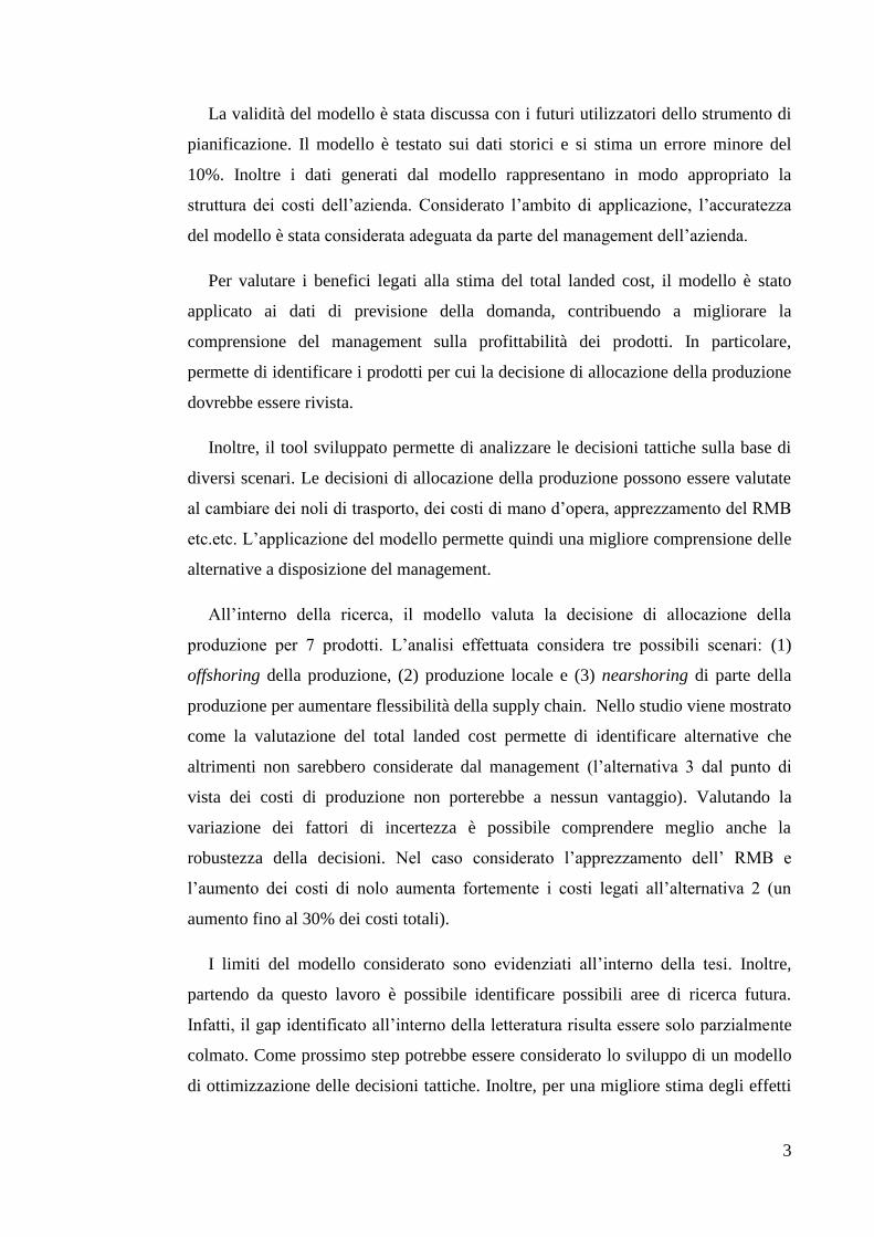


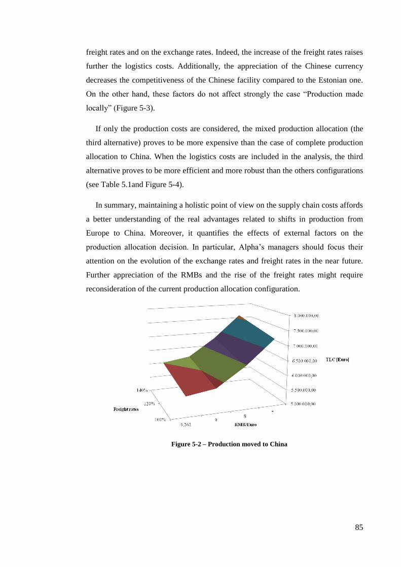


![Yiwen Hua , Pritish , Saravana , and arXiv:2003.11172v1 ... · Holopix50k: A Large-Scale In-the-wild Stereo Image Dataset Yiwen Hua[0000 0003 2334 7157], Puneet Kohli[0000 0002 4817](https://static.documents.pub/doc/80x56/5f89872fdddb812f8122e639/yiwen-hua-pritish-saravana-and-arxiv200311172v1-holopix50k-a-large-scale.jpg)

![YIWEN DING arXiv:1511.06882v1 [math.NT] 21 Nov 2015 · YIWEN DING Abstract. We study some closed rigid subspaces of the eigenvarieties, constructed by using the Jacquet-Emerton functor](https://static.documents.pub/doc/80x56/60a1bcc7de51db59d4464acf/yiwen-ding-arxiv151106882v1-mathnt-21-nov-2015-yiwen-ding-abstract-we-study.jpg)


