Page 1
Milano-2012
POLITECNICO DI MILANO
PhD School
Doctoral Program in Electrical Engineering
Cycle XXIV
Optimized Antenna for Low UHF Band Wireless
Power Transfer (WPT)
PhD Candidate: Supervisor:
Houriyeh Shadmehr Prof. Riccardo Zich
The Chair of the Doctoral Program: Tutor:
Prof. Alberto Berizzi Prof. Gabrio Superti Furga
Page 2
My dream would not come true without them.
I did not know who would have become today without
them.
Dedicate to my parents with love.
Page 3
I
Acknowledgement
Success is a science, if you have the conditions, you will get the results.
”Oscar Wilde”
I would like to express my deepest gratitude to all those who provided me the condition
to approach to my goal.
Foremost, I want to thank my supervisor Prf. Riccardo Zich who believed and trusted to
my abilities to finish my doctoral study; who his support helped me overcome many
crisis situation and problems. I am deeply grateful Dr. Marco Mussetta for being always
there to listen and give advice, for long discussions that helped me sort out the technical
details of my work.
I would also like to thank Dr. Francesco Grimaccia and Dr. Morris Brenna for their
encouragement and comments during this work.
I would especially like to thank Dr. Federica Foiadelli- my angel - who gave me hope in
the darkness period of my life.
Finally, I want to thank to the department of Energy, committee members, and my
coordinator Prf. Alberto Berizzi for his support.
Page 4
Summary
II
Summary
Delivering power without requiring wire is an advance in transferring power
technology; and it is named Wireless Power Transfer (WPT). Wireless power transfer
makes possible to overcome drawback of conventional power transfer with wires, due to
the wire resistance, wire routing, and so on; re-charging cell phones, game controllers,
laptop, mobile robots, and electrical vehicles without being plugged in; making more
reliable industrial systems and medical devices by eliminating trouble prone wiring and
replaceable batteries; transmitting power in safe mode for human body and animals;
providing continuous and instantaneous power transfer; and to miniaturize electrical
systems and devices. Such advantages promote the interest of scientists, engineers, and
researchers in studying and using wireless power transfer.
At present, the power is delivered wirelessly by employing such diverse physical
mechanisms as: Radio Frequency (RF), and Resonance Inductive Coupling.
Radio Frequency: Recently, the availability of wireless standards for huge number of
applications, from mobile phones, smart phones, to always-on WLAN devices shifted
the attention on the extraction of energy from EM fields in the RF band. On other hand,
Energy Harvesting Technology (EHT) allows to scavenge small amount of power from
human activities or environment heat, light, vibration or Electromagnetic Field (EF). By
availability the EM field in our daily life and using Energy Harvesting technology,
nowadays the power is extractable from EM in RF range, and named Radio Frequency
(RF) energy harvesting and it has the resulting benefit to product design (e.g.
miniaturizing biomedical implanted devices and power supply), transfer power
wirelessly over distance (e.g. Solar Power Satellite), in self-powering, where requires
continuously available power source with lifespan (e.g. Wireless Sensor Network), and
Page 5
Summary
III
so on. Furthermore, RF Energy Harvesting provides the possibility of recycling EM
radiation in the free space and using it as an alternative supply source that leads to
reduce of the EM field pollution, miniaturization of the energy harvesting system with
respect to energy harvesting system based on the other energy sources (e.g. large size of
a photovoltaic).
One of the most important components in RF power harvesting system is called
rectenna which is composed of a receiving antenna and rectifier. The receiving antenna
plays a critical role in RF energy harvesting system, since it must extract the power
from radiated electromagnetic waves.
Resonance Inductive Coupling: in this mechanism, resonance is used to deliver power
wirelessly, by tuning transmitter and receiver at mutual EM frequency. coupling
transmitter and receiver in resonant way has two main profits: exchange power
efficiency without much leakage (minimizing energy leakage causes the maximization
in the transferred energy to the receiver), and improve power efficiency over distances.
Inductive coupling techniques have been reported to have high power transfer
efficiencies (on the order of 90%) for very short lengths (1-3cm). However, the power
efficiency of such technique decreases for longer distance drastically.
The biggest challenge in the design of RF energy harvesting system (rectenna) and
wireless power transmitting systems via Resonance Inductive Coupling is the
maximization of the transferred energy to the receiver, reduction of the size, and
transmitting power in safe mode for human body and animals. This is possible by
suitably redesigning the transmitting and receiving devices, trying to find the correct
shape that allows on rising in performance, and tuning the transmitter and receiver at
EM frequency to decrease leakage.
In this work, an approach based on a novel evolutionary technique is proposed for the
design of loop wire antenna configuration, with the aim of increasing the transfer
Page 6
Summary
IV
efficiency, the robustness of the coupling, and minimizing the average power loss, and
miniaturization.
The new hybrid approach here proposed, called Genetical Swarm Optimization (GSO),
and consists in a strong co-operation of Genetic Algorithm (GA) and Particle Swarm
Optimization (PSO). In particular, a key feature of the algorithm is that it maintains the
integration of GA and PSO for the entire run. In each iteration, the set of solutions is
divided into two parts and it is evolved with two techniques respectively. It is then
recombined in the updated population for the next iteration; after that it is again divided
randomly into two parts in the next run, in order to take advantage of both genetic and
particle swarm operators. The population update concept can be easily understood
thinking that a part of the individuals has been substituted by new generated ones by
means of GA, while the remaining are the same of the previous generation but have
been moved on the solution space by PSO. This kind of updating results in a more
“natural” evolution, where individuals not only improve their score for natural selection
of the fitness, or for good-knowledge sharing, but for both of them at the same time.
A driving parameter is introduced for the GSO algorithm, called Hybridization
Coefficient (HC); it expresses the percentages of population that in each iteration is
evolved with GA: so HC=0 means the procedure is a pure PSO (the whole population is
processed according to PSO operators), HC=1 means pure GA(the whole population is
optimized according to GA operators), where 0<HC<1 means that the corresponding
percentage of the population is developed by GA, while the rest with PSO technique.
The output of the evolutionary optimization method or on other words, the candidate
design is simulated at frequency range 450MHz- 600MHz by Matlab simulation in
order to investigate the properties of the candidate design. Rao-Wilton-Glisson basis
function and delta-gap feed model have been used to create a system of moment
equations (Method of Moment) in home-built Matlab simulation tool. A wire is
represented with the use of a thin strip model having one RWG edge element per strip
width. The strip width should be four times of the wire radius. As the last step, the
Page 7
Summary
V
results obtained by Matlab are compared with the obtained results by FEKO- Lite
(commercial software) to check and verify the reliability of the obtained results by
Matlab for optimized antenna.
In this study, a novel antenna by means of optimization loop wire base on fractal
variation has been proposed for application in WPT devices and RF energy harvesting
component. The presented optimization approach is based on a recently developed
evolutionary method. The design procedure is well suited in order to increase the
transfer efficiency and the robustness of the coupling, with the aim of minimizing the
average power loss and the size of the WPT systems.
Finally, Numerical results simulated with home-mode MoM-Matlab code have been
verified by comparison with full-wave commercial simulator, FEKO-Lite.
Page 8
Index
Index
Acknowledgement………………………………………………………………………………...I
Summary………………………………………………………………………………………….II
Chapter 1 Introduction ................................................................................................ 1 1.1 History of Wireless Power Transfer........................................................................................... 3
1.2 Radio Frequency Technology.………………………………………………………………… 4
1.3 Resonance Inductive Coupling .................................................................................................. 7
1.4 Field-to-Wire Coupling ........................................................................................................... 11
1.5 Antenna Design and Optimization Technique ........................................................................ 16
Chapter 2 Numerical Method-Matlab ............................................................................................. 18
2.1 Introduction .............................................................................................................................. 18
2.2 Antenna Theory ....................................................................................................................... 18
2.3 Matlab Code ............................................................................................................................ 19
2.4 Antenna structure .................................................................................................................... 20
2.5 Impedance Matrix and Surface Current .................................................................................. 23
2.6 Code Sequence ........................................................................................................................ 28
2.7 Electrically Large Loop Antenna ............................................................................................ 28
Chapter 3 Optimization Method ...................................................................................................... 31
3.1 Introduction ................................................................................................................. 31
3.2 Genetic Algorithm ...................................................................................................... 33
3.3 Particle Swarm Optimization ...................................................................................... 34
3.3.1 Traditional PSO Implementation ....................................................................... 34
3.3.2 Some Consideration on PS................................................................................. 37
3.4 The Class of Meta-Swarm Algorithm ......................................................................... 38
3.4.1 Undifferentiated Meta-Swarm ........................................................................... 39
3.4.2 Differentiated Meta-Swarm ............................................................................... 41
Page 9
Index
3.5 Genetical Swarm Optimization ................................................................................... 44
3.5.1 The GSO Algorithm Class ................................................................................. 47
3.5.2 Preliminary Analysis .......................................................................................... 49
3.5.3Performance Analysis………………………………........................................ 54
Chapter 4 Design and Numerical Results ................................................................................ 58
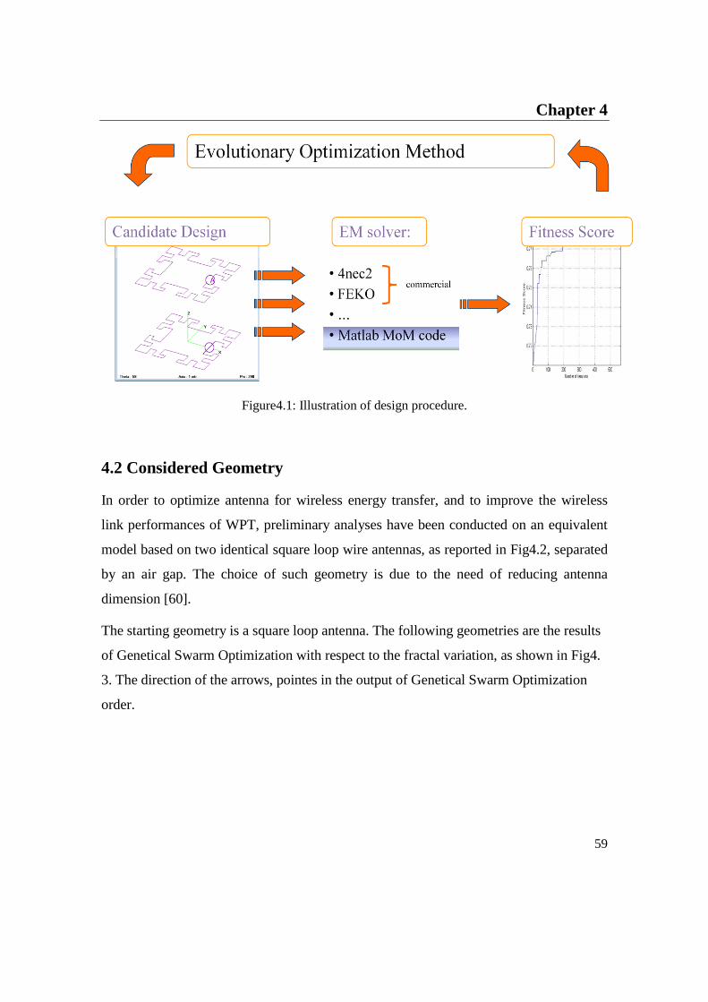
4.1 Introduction ................................................................................................................. 58
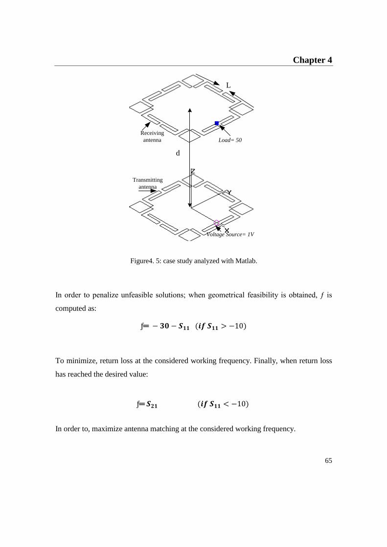
4.2 Considered Geometry ................................................................................................. 59
4.3 Simulation Analysis .................................................................................................... 61
4.3.1 Antenna Optimization Procedure .......................................................................... 63
4.4 Distance and Power Gain ............................................................................................ 67
4.5 Frequency Analyzing .................................................................................................. 72
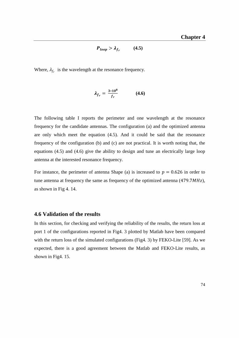
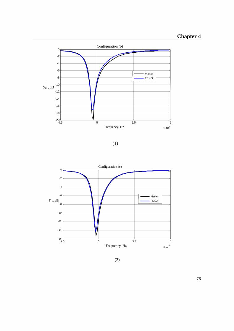
4.6 Validation of the Results ............................................................................................. 74
Chapter 5………………………………………………………………………………………. 78
Conclusion……………………………………………………………………………… 78
References……………………………………………………………………………………... 81
Page 10
Chapter1
1
Chapter1
Introduction
Delivering power without requiring wire is an advance in transferring power technology
and named Wireless Power Transfer/transmitting (WPT). Thus, Wireless power
Transfer (WPT) as the name shows is the transfer of power ranging from milliwatts to
kilowatts over a distance range from centimeters to several meters without
interconnecting. Wireless power transfer makes possible to overcome drawback of
conventional energy/power-transfer power with wires- due to the wire resistance, wire
routing, and so on. Other benefits of the power transfer wirelessly include: re-charging
cell phones, game controllers, laptop, mobile robots, and electrical vehicles without
being plugged in, making more reliable industrial systems and medical devices by
eliminating trouble prone wiring and replaceable batteries, transmitting power in safe
mode for human body and animals, providing continuous and instantaneous power
transfer, and to miniaturize electrical systems and devices. Such advantages promote the
interest of scientists, engineers, and researchers in studying and using wireless power
transfer.
Wireless Power Transfer (WPT) is made possible by various technologies, whereas
conventional power transmitting is solely used wire technology to deliver power. The
technologies and methods of WPT are as the following:
Inductive Coupling
The transfer of power takes place by electromagnetic coupling through a process
known as mutual induction. The simplest example of the inductive coupling is
Page 11
Chapter1
2
transformer. The primary and secondary coils of transformer are connected base on
principles of electromagnetism. For instance, the battery charge of a mobile phone
and electric toothbrush are powered by this technology.
However, the main drawback of this technology is the short distance. The receiver
must be kept very close to the transmitter.
Resonance Inductive Coupling
The resonance inductive coupling technology is presented in order to overcome the
main drawback of non-resonance inductive coupling technology.
The resonance inductive coupling is combination of inductive coupling and
resonance frequency. Receiver and transmitter are tuned to mutual electromagnetic
frequency. Resonance causes two resonance objects of the same resonance
frequency interact very strongly and increases the transfer efficiency with respect to
the distance range. A common use of the technology is for powering contactless
smart cards.
Radio Frequency and Microwave Power Transmission
High amount of the power is delivered over the long distance by converting into
microwaves; the transmitting point and receiving point must be in the line of sight.
The process of Microwave WPT is as the following:
1. Electrical energy to microwave energy.
2. Capturing microwaves by using rectenna.
3. Microwave energy to electrical energy.
One of the applications of Microwave WPT is in Solar Power Satellite. A satellite with
solar panels is sent to orbit the earth and collect the sunlight. The satellite generates the
electrical power with using solar cells. This energy is then converted into the microwave
power and transmitting to the receivers of rectenna on the earth. At the end of the
process, the microwave energy is converted back into electrical energy in the rectifier of
rectenna. The similar procedure is employed to capture power from electromagnetic
field at radio frequency band.
Page 12
Chapter1
3
Laser Power Transmission
Laser method of wireless power transfer is used a coherent light beam to transport very
high power point to point in a line of sight. In this technology, the size of the antenna
could be much smaller, and the light could be diffracted by atmospheric particles easily.
In this thesis, we focused on Radio Frequency Energy Harvesting and Resonance
Inductive Coupling technologies. We proposed a novel hybrid technique of optimization
in order to redesign and enhance the elements of the system of those technologies.
The chapter is started with a brief review on the history of the wireless power
delivering, and the following sections have been devoted to describe Radio Frequency
and Resonance Inductive coupling technologies in transferred power wirelessly in
details.
1.1 History of Wireless Power Transfer
In the early 1900’s, the physicist Nikola Tesla conceived and explored the idea of the
wireless power transmitting. Tesla managed to build a giant coil in a large square
building over rose a 60 m mast with a 1m diameter copper ball positioned at the top.
The coil was resonated at a frequency of 150 KHz and was fed with 300 kw of low-
frequency power obtained from the Colorado Springs electric Company. As well, he
succeeded to power the fluorescent lamps 25 miles from the power source without using
wires. Nevertheless, Tesla’s work was never commercially exploited due to the
dangerous nature of the experiments, low efficiency on power transfer, and mainly by
the deletion of financial resources. However, the work of Tesla was based on very long
wavelength.
W. Brown was the first engineer who approached to use microwave and radio waves for
effective power transmitting through long distances, in 1660’s. The most research in this
field focused on rectennas (J. A. G Akkermans & Visser-2005, Mohammad Ali &
Page 13
Chapter1
4
Dougal-2005, Ren and Chang-2006, Shams & Ali-2007), which are antennas capable to
collect energy from radio waves.
NASA for the first time in 2003 proposed a scheme to power satellites and wireless
energy transfer by utilizing laser mechanism. The laser beam is capable to deliver very
high energies in a line of sight. The laser mechanism is efficient to send power point to
point, but it is dangerous mechanism for living beings.
Nikola Tesla’s laboratory in Colorado Springs
Over the years, the idea of Tesla, wireless power delivery have been conceived, tried,
and tested by many (Glaser, 1968; McSpadden et al., 1996; Shinohara & Mastsumoto,
1998; Strassner & Chang, 2002; Mickle, et al., 2006; Conner, 2007).
1.2 Radio Frequency Technology
Energy harvesting (EH) is the process of capturing and converting energy into usable DC
voltage for items as small as cell phone or as large as satellites. There are various energy
Page 14
Chapter1
5
sources for energy harvesting technology. For instance, ambient energy sources (e.g. Solar;
Wind; Biomass; Hydro geothermal; and Tides) or handmade-man ambient energy (e.g. emitted
Electromagnetic waves (EM) from TV signals; wireless radio networks; and cell phone towers)
[1]. Recently, the availability of wireless standards for huge number of applications,
from mobile phones, smart phones, to always-on WLAN devices shifted the attention on
the extraction of power from EM fields in the RF band [2]. On other hand, there is the
possibility of recycling EM radiation in the air and use it as an alternative supply source
by EH technique. In additional, scavenging the power from EM can allow to reduce the
size of the harvesting system with respect to energy harvesting system based on the
other energy sources (e.g. large size of a photovoltaic) [3].
Therefore, extraction power from electromagnetic waves to power devices is called Radio
Frequency (RF) energy harvesting. RF power harvesting technology has the resulting benefit to
product design (e.g. miniaturizing biomedical implanted devices and power supply); transfer
power wirelessly over distance (e.g. Solar Power Satellite); in self-powering; where requires
continuously available power source with lifespan (e.g. Wireless Sensor Network); and so on.
Fig.1.1 shows the block diagram of a RF energy harvesting system. The system operates
as: an antenna-receiving antenna picks up the incidence electromagnetic wave at RF
band and then the picked RF wave is converted to a DC voltage via rectifier. The DC
voltage is stored or used to power devices. In order to reduce the transmission loss and
increase the voltage gain, the matching network between receiving antenna and rectifier
is necessary [4, 5].
As been seen, the heart of a RF energy harvesting system is composed of a receiving
antenna and rectifier that their composition is named “rectenna”. Hence, the main
research fields focus on rectenna [6, 7, 8, and 9]. Since the role of the receiving antenna
is, extraction the power from the radiated electromagnetic wave, rectifier’s role is
conversion the picked power by antenna to the useful DC voltage. For enhancement of
the performance of the RF energy harvesting, the receiving antenna and rectifier must
be optimized and redesigned.
Page 15
Chapter1
6
Figure1.1: Schematic of RF energy harvesting systems.
Many works could achieve sufficient power but provided low output voltage, which
made them inadequate for using in some application [10] such as: passively powered
wireless sensor networks. In addition, some previous studies have proposed a new
design of the rectifier in order to increase the efficiency of the RF-DC conversion and
recoverable power.
As been known, the power density decreases over longer distance. Thus, it is essential
that the RF-DC conversion circuit be able to operate at very low receiver power. To
overcome this, an optimized rectifier circuit has been introduced and the minimum-
threshold of the RF-DC conversion has been improved [11].
In [12], in order to optimize the RF energy harvesting system, author has been
employed a DC/DC voltage boost converter for elevation the voltage level. Moreover,
author has been used a patch antenna array as collecting the RF power from the
incidence electromagnetic waves with efficiency of 85% at 1.8 GHz.
However, in this work, we are more interested in raising the receiving antenna gain and
we will address this case.
Page 16
Chapter1
7
1.3 Resonance Inductive Coupling
The mechanism resonance is used to deliver power wirelessly by tuning transmitter and
receiver at mutual EM frequency; and coupling transmitter and receiver in resonant way
has two main profits: exchange power efficiency without much leakage (minimizing
energy leakage causes the maximization in the transferred energy to the receiver), and
improve power efficiency over distances.
Inductive coupling techniques have been reported to have high power transfer
efficiencies (on the order of 90%) for very short lengths (1-3cm) [13]. However, the
power efficiency of such technique decreases for longer distance drastically. Many
works have been done on increasing power efficiency of such technique with respect to
longer distances [14, 15, and 16]. In all those mentioned works, authors have developed
a design, which consists of two helices and two singl loops [17]; as shown in Fig1. 2. In
[14], authors have optimized the typical Strongly Coupled Magnetic Resonance, which
has been illustrated in Fig1. 2. They are managed to achieve efficiencies 90.2% for
15cm distance to 35% for 45cm distance and increase the efficiency of the wireless
power transfer to compare with conventional inductive coupling [18] and conventional
Strongly Coupled Magnetic Resonance designs [19]. The same authors have analyzed
the geometrical parameters of the SCMR and they showed that, the optimized SCMR in
their previous work has a wide range of local optimum. Moreover, when they launched
the system on that optimal range, the system reached the maximum efficiency [15]. In
[16], the efficiency of wireless power transfer via magnetic resonance has been
improved by using transmission coil array. Although, the previous works could have
improved the power gain over larger distance, but they still require more work with
respect to the size of the proposed model for resonance magnetic coupling. Because, in
some applications such as implantable medical devices the size of the suggested model
or system plays a key role. In additional, that is an important term in design of the
electrical devices and systems.
Page 17
Chapter1
8
Therefore, present a model for Resonance Inductive Coupling technology that could
meet the three requirements: a) high efficiency, b) small size, and c) longer air gap,
make the technology more adequate for more applications for instance: RFID,
biomedical implant devices, and electrical car charging.
Source Element Load Element
Transmitting Element Receiving Element
Figure1. 2: Schematic of an SCMR power transfer system. (From [17]).
Charging Electrical Vehicles with Resonance Inductive Coupling
Technology
Resonance Inductive Coupling technology could introduce a convenient charging
system for EVs and it makes possible to charge the vehicles, as they are parked in the
parking or in your house’s garage automatically without requiring of plugging and cord.
Powering vehicles by electricity is a new challenge in transportation technology.
Nowadays, the attention of some scientists, researchers, and engineers have been
attracted to EVs due to various advantages of EVs technology including: electric-
Page 18
Chapter1
9
powered vehicles are more economical than gas-powered vehicles, specially their
electricity could be provided from renewable resources such as Solar, Wind, and so on;
electric-powered vehicles pollute less than gas-powered vehicles, they are much reliable
and require less maintenance to compare with gas-powered vehicles, and they can
reduce the energy dependency.
In general, an electric motor and controller propel EVs; controller supplies the power of
electric motor and obtains its required power from a rechargeable battery. Hence, the
batteries are the heart of EVs, since the batteries should be powerful and long-lasting
enough to move vehicles with minimum of recharging. As aforementioned, Resonance
Inductive Coupling is a technology, which has been developed recently for charging
batteries of the EVs. Inductive charging makes possible to charge EVs stationary and
roadway electrification.
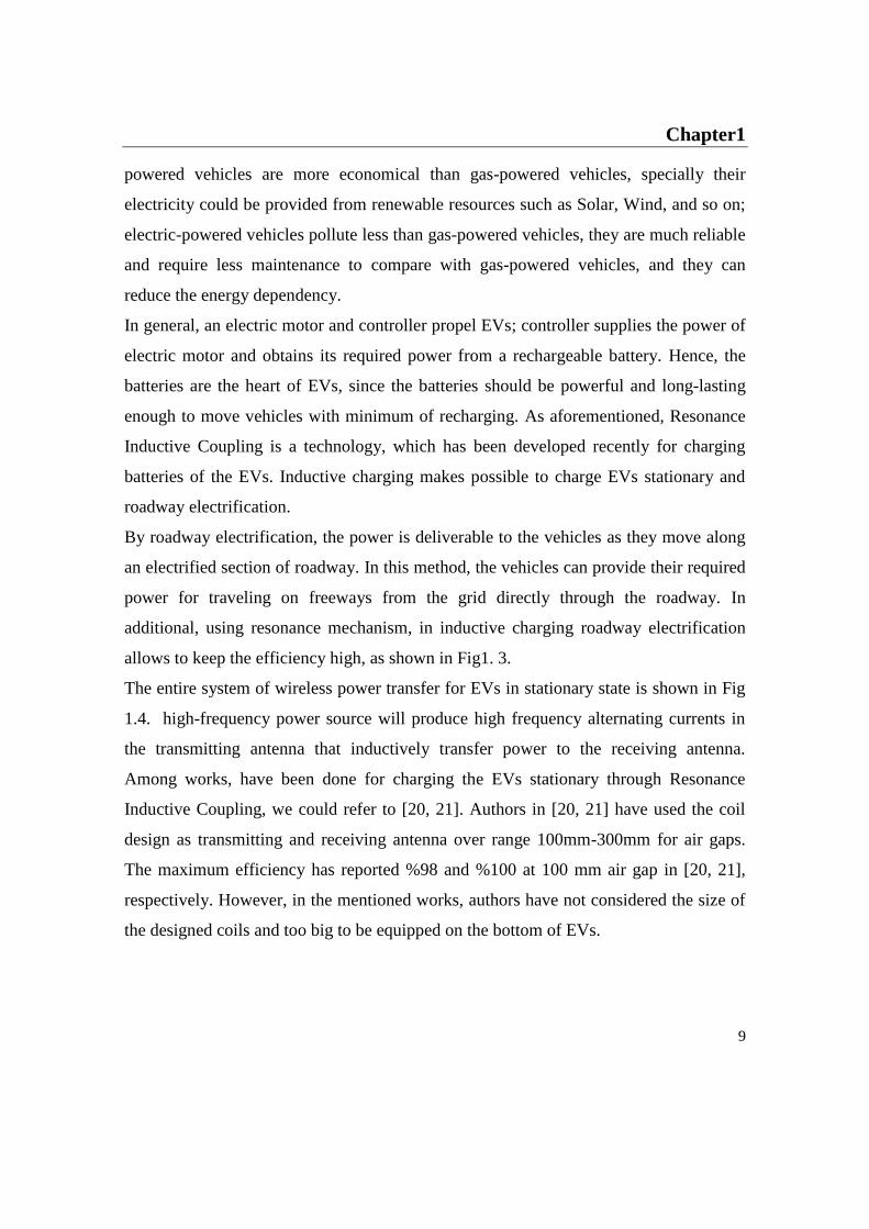
By roadway electrification, the power is deliverable to the vehicles as they move along
an electrified section of roadway. In this method, the vehicles can provide their required
power for traveling on freeways from the grid directly through the roadway. In
additional, using resonance mechanism, in inductive charging roadway electrification
allows to keep the efficiency high, as shown in Fig1. 3.
The entire system of wireless power transfer for EVs in stationary state is shown in Fig
1.4. high-frequency power source will produce high frequency alternating currents in
the transmitting antenna that inductively transfer power to the receiving antenna.
Among works, have been done for charging the EVs stationary through Resonance
Inductive Coupling, we could refer to [20, 21]. Authors in [20, 21] have used the coil
design as transmitting and receiving antenna over range 100mm-300mm for air gaps.
The maximum efficiency has reported %98 and %100 at 100 mm air gap in [20, 21],
respectively. However, in the mentioned works, authors have not considered the size of
the designed coils and too big to be equipped on the bottom of EVs.
Page 19
Chapter1
10
Figure1.3: Electrified roadway concept.
Figure1.4: Concept of wireless power transmitter for EVs.
This brings a new issue for car designers. Hence, in this study our aim is also to propose
a model of antenna in resonance inductive coupling, with regard to the characteristic of
antennas and its relation with power efficiency.
Page 20
Chapter1
11
1.4 Field-to-Wire Coupling
In this section, we address the topic from different point of view and try to model the
problem by equivalent circuits.
In Electromagnetic Compability field, the most effort of EMC engineers is to reduce
electromagnetic interference and enhance performance of electronic devices in vicinity
of interference. In order to that, some qualifications evolve to check the quality of the
electronic devices; such as radiated emission and susceptibility.
Radiated Emission
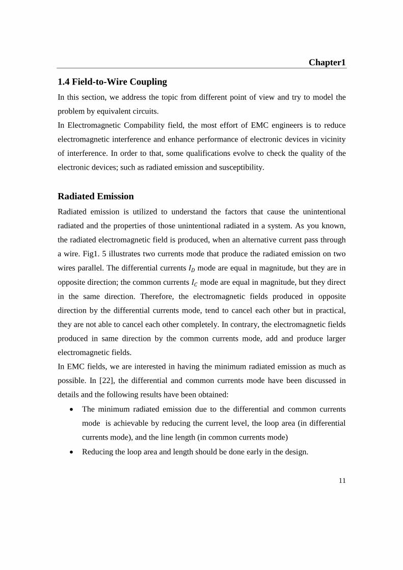
Radiated emission is utilized to understand the factors that cause the unintentional
radiated and the properties of those unintentional radiated in a system. As you known,
the radiated electromagnetic field is produced, when an alternative current pass through
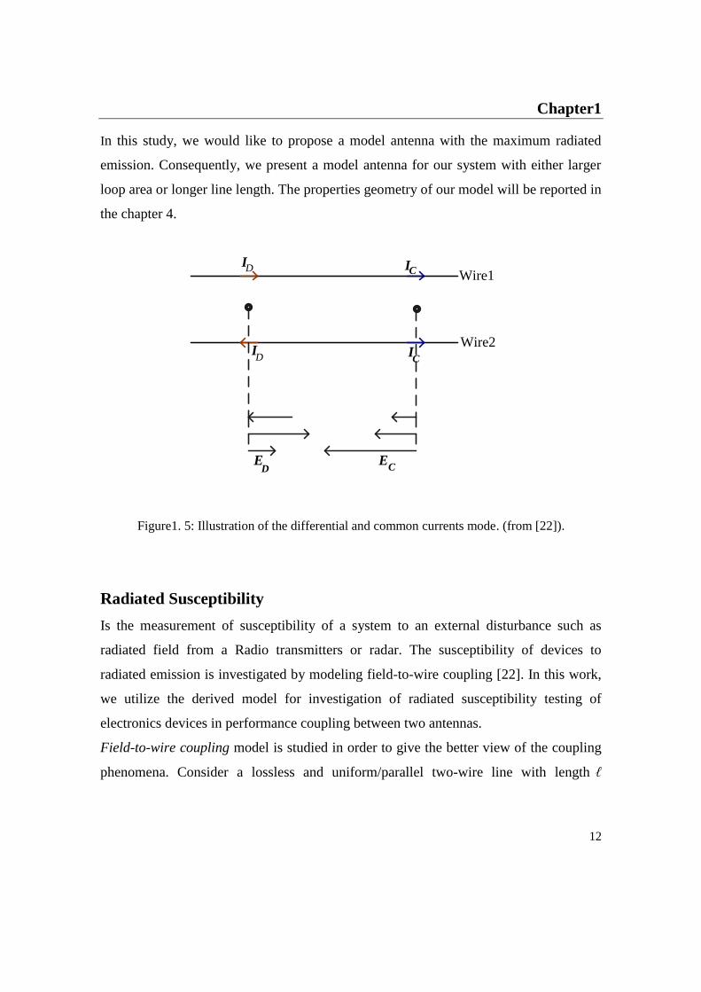
a wire. Fig1. 5 illustrates two currents mode that produce the radiated emission on two
wires parallel. The differential currents 𝐼𝐷 mode are equal in magnitude, but they are in
opposite direction; the common currents 𝐼𝐶 mode are equal in magnitude, but they direct
in the same direction. Therefore, the electromagnetic fields produced in opposite
direction by the differential currents mode, tend to cancel each other but in practical,
they are not able to cancel each other completely. In contrary, the electromagnetic fields
produced in same direction by the common currents mode, add and produce larger
electromagnetic fields.
In EMC fields, we are interested in having the minimum radiated emission as much as
possible. In [22], the differential and common currents mode have been discussed in
details and the following results have been obtained:
The minimum radiated emission due to the differential and common currents
mode is achievable by reducing the current level, the loop area (in differential
currents mode), and the line length (in common currents mode)
Reducing the loop area and length should be done early in the design.
Page 21
Chapter1
12
In this study, we would like to propose a model antenna with the maximum radiated
emission. Consequently, we present a model antenna for our system with either larger
loop area or longer line length. The properties geometry of our model will be reported in
the chapter 4.
Wire1
Wire2
ID
I I
I
D
C
C
E ED C
Figure1. 5: Illustration of the differential and common currents mode. (from [22]).
Radiated Susceptibility
Is the measurement of susceptibility of a system to an external disturbance such as
radiated field from a Radio transmitters or radar. The susceptibility of devices to
radiated emission is investigated by modeling field-to-wire coupling [22]. In this work,
we utilize the derived model for investigation of radiated susceptibility testing of
electronics devices in performance coupling between two antennas.
Field-to-wire coupling model is studied in order to give the better view of the coupling
phenomena. Consider a lossless and uniform/parallel two-wire line with length ℓ
Page 22
Chapter1
13
radius 𝑟𝑤 , and separation by distance ℎ . Uniform/parallel transmission line is assumed
to be excited by an external plane wave, as shown in Fig1.6.
The two-conductor line is assumed electrically short at the frequency of interest. This
leads to model the line with per-unit-length parameters of inductance 𝑙 and capacitor 𝑐,
whereas the effects of the external field are presented by distributed voltage and current
along the line [22]. Distributed voltage 𝑉 and current 𝐼 are related to the normal
magnetic field component and the transverse electric field component, respectively [22].
As long as the termination impedances are not extreme values such as short or open
circuit, the line inductance and capacitance are neglected.
The equivalent circuit has been shown in Fig.1.6b. Under this condition, the Thèvenin
voltage of the equivalent circuit of the line (Fig1.6b), at where the non-linear load is
located, is derived, as shown in Fig1.6c. The voltage at points 𝐴𝐵, as the loads are
matched, is obtained as
𝑽𝑨𝑩 = 𝟏
𝟐𝒋ω𝓵𝒉 𝝁𝟎𝑯 + 𝒁𝒄
𝝅𝜺𝟎
𝐥𝐧 𝒉
𝒓𝒘 𝑬 , 𝒁𝒍 = 𝒁𝒄 = 𝒁𝒏 (1.1)
Where, 𝐻 = ∣𝐸∣
𝑛0, and 𝑛0 = 𝜇0𝑐0 impedance of free space. In order to predict incidence
field picked-up of a two-conductor line ∣ 𝑉𝐴𝐵 ∣ is plotted against frequency, as shown in
Fig1.7. Specific values adopted for above model are listed in the following:
𝓵 = 𝟏𝟎𝒄𝒎
𝒉 = 𝟑𝒄𝒎
𝒓𝒘 = 𝟎. 𝟓𝒎𝒎
𝒇𝒓𝒆𝒒𝒖𝒆𝒏𝒄𝒚 = 𝟎. 𝟗𝑮𝑯𝒛 − 𝟐𝑮𝑯𝒛
∣ 𝑬 ∣= 𝟏𝒗/𝒎
Page 23
Chapter1
14
Source of
Radiation
(a)
(b)
Page 24
Chapter1
15
(c)
Figure1.6: (a) A uniform/parallel two-wire line excited by an external electromagnetic wave, (b)
circuit representation for one section of the line, and (c) Thèvenin equivalent circuit at where the
non linear load is located.
Incidence uniform plane wave is considered with endfire incidence.
Figure1.7: ∣ 𝑉𝐴𝐵 ∣ versus frequency.
Page 25
Chapter1
16
1.5 Antenna Design and Optimization Technique
Therefore, the biggest challenge in the design of RF energy system (rectenna) and
wireless power transmitting systems is the maximization of the transferred energy to the
receiver in order to increasing their performance of these technologies. This is possible
by suitably redesigning the transmitting and receiving devices, reduction of the size,
trying to find the correct shape that allows on rising in performance, and tuning the
transmitter and receiver at EM frequency to decrease leakage, and transmitting power in
safe mode for human body and animals. With this aim an approach based on a novel
evolutionary technique is proposed for the design of an optimized antenna
configuration.
As been known, when two antennas are placed closely, a coupled mode resonance
phenomena are created between them. In order to maximize delivering power, the
radiation antennas should be reduced. As well as, the distance between antennas is short
with respect to the wavelength; if the distance between antennas could be extended over
such coupled mode phenomena, they would benefit a number of applications. In this
study, we chose loop wire antenna as structure for optimization due to several reasons:
a) loop wire antennas are common structure in wireless power transfer system [23, 24],
b)they have greater efficiency than monopole or dipole antennas in case of being
electrically large, c) and they are useable in low-power short-range transmitter [25, 26].
Evolutionary optimization algorithms are global search techniques, thus they can
overcome the drawbacks of the traditional optimization methods: in fact, they can face
nonlinear and discontinuous problems, with a great number of variables. Among the
main evolutionary optimization approaches, it is worth mentioning the Genetic
Algorithm (GA) and the Particle Swarm Optimization (PSO).
In this work, a novel hybrid technique, named Genetic Swarm Optimization (GSO), is
used: several comparative studies over different optimization tasks have shown the
effectiveness of Genetic Swarm Optimization in exploring the problem hyperspace,
Page 26
Chapter1
17
especially for the optimization of large domain objective functions; moreover, GSO has
been already successfully applied to the optimization of antennas, wireless systems and
energy harvesting devices [27,28], usually allowing to reduce the number of iterations,
and thus the computational effort, requested to optimize complex EM problems.
Page 27
Chapter 2
18
Chapter 2
Numerical Method-Matlab
2.1 Introduction
A wire antenna is treated as one-dimensional segment model. Requirement theory
behind of this model is a special integral equation. Too large ratio of the radius to the
length in one-dimensional segment model causes some problem. Hence, to avoid this
problem, Matlab is used to investigate the properties of the antenna under analysis. A
wire is represented by a thin strip model having one RWG edge element for strip width;
the width of the strip should be four times the wire radius [29].
2.2 Antenna Theory
Two methods that in the last three decades have been more successful in the analysis of
many intractable antenna problems are the Integral Equation (IE) method and the
Geometrical Theory of differential (GTD).
The Integral Equation method describes the solution of the antenna problems in form of
an integral, where the induced current density is usually unknown and part of the
integral. Then, Method of Moments (numerical technique) are used to solve the
unknown induced current density. Afterwards, the radiation integrals are used to find
the radiated fields and other systems parameters. These parameters include:
Antenna near field
Antenna far field
Page 28
Chapter 2
19
Surface current distribution
Input impedance and return loss
Antenna transfer function and antenna-to-antenna link
There are two types of IE’s: one is the Electric Field Integral Equation (EFIE), another
one is the Magnetic Field Integral Equation (MFIE). Electric Field Integral Equation is
convenient for wire-type antenna; whereas Magnetic Field Integral Equation is only
valid for closed surfaces. Standard Matlab package is applied in order to solve and
simulate the Integral Equation (to find the solution of the unknown induced current
density) by using the Method of Moments. Rao-Wilton-Glisson (RWG) basis functions,
the electric field integral, and the feeding –edge model are the background materials of
the underlying Method of Moments (MOM) code.
2.3 Matlab Code
In Matlab, the numerical steps of the moment method (MM) are calculated by Matlab
source codes and the antenna mesh generator files, successively. It is worth nothing that
these codes are executed sequentially.
There are two main Matlab scripts. The first script impmet.m computes the impedance
matrix 𝑍 [29] in order to determine electric current distribution on the antenna surface,
and it is the basic and the most important step of the moment method. The second script
point.m computes the radiated field of an infinitesimally small electric dipole or a group
of dipoles at any points in space. This code allows us to determine the near and far field
of an antenna. If the both mentioned scripts are programmed correctly, the rest of the
work usually does not constitute any difficulties. The rest of Matlab codes are used to
support and visualize the input and output data for an antenna. Those codes that their
names start with rwg, e.g., rwg1.m, rwg2.m, rwg3.m are associated with the antenna
Page 29
Chapter 2
20
structure operations. Those codes that their names start with efield such as efield1.m,
efield2.m, efield3.m are associated with the near and far field antenna parameters.
2.4 Antenna Structure
Antenna structures can be built in Matlab with two different ways. One way is the built-
in mesh generator of the Matlab PDE toolbox (type command pdetool on workspace of
Matlab). In this way, the mesh generator uses the convenient Graphical User Interface
(GUI) to create planar structures of any rectangles, polygons, and circles. The design is
able to be a 3D structure by writing a short script involving the 𝑧-coordinate
dependency. For instance, a planar rectangle is created by PDE toolbox, as shown in
Fig2.1.
An unstructured mesh could be created either by clicking on the ∆ button on the top of
the PDF Toolbox window or by selecting Initialize Mesh from the mesh menu. In order
to have a structured mesh, selecting parameters option from the mesh menu and typing
“inf” at maximum edge size part. Afterward, refine the mesh several times to obtain the
structured mesh. Fig2. 2 represents unstructured and structured mesh for a circle with
one diameter in PDE window.
The Second way is base on identifying the boundary of the antenna structure
analytically. Matlab function Delaunay and function Delaunay3 are used respectively, to
create mesh to the structure and to approach 3D structure. The advantage of this way is
that 3D antenna surface and volume meshes are created arbitrary and the PDE toolbox is
not requirement any longer. In this work, we utilized the strip mesh. The strip mesh is
defined by cell size and strip width. Each cell is divided to two triangles by drawing the
chord of the cells. The accuracy of the mesh depends on the number of the triangles.
Obviously, we are able to obtain precise results by increasing the number of the
triangles.
Page 30
Chapter 2
21
(a)
(b)
Figure 2.1: Two plate meshes create in PDE window: (a) Unstructured mesh; (b) Structured
Mesh.
Page 31
Chapter 2
22
(a)
(b)
Figure2. 2: created circle with: (a) Unstructured mesh; and (b) Structured Mesh.
Page 32
Chapter 2
23
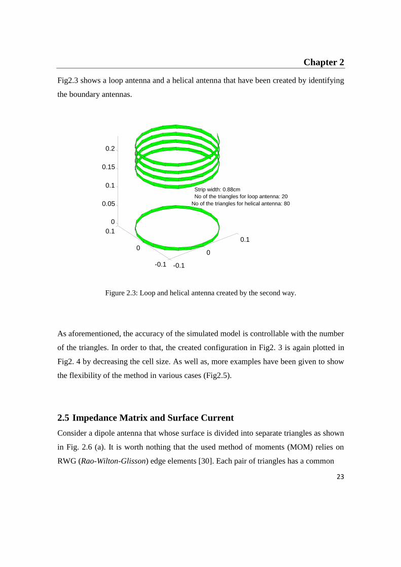
Fig2.3 shows a loop antenna and a helical antenna that have been created by identifying
the boundary antennas.
Figure 2.3: Loop and helical antenna created by the second way.
As aforementioned, the accuracy of the simulated model is controllable with the number
of the triangles. In order to that, the created configuration in Fig2. 3 is again plotted in
Fig2. 4 by decreasing the cell size. As well as, more examples have been given to show
the flexibility of the method in various cases (Fig2.5).
2.5 Impedance Matrix and Surface Current
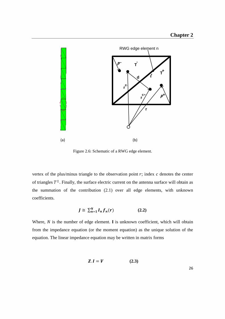
Consider a dipole antenna that whose surface is divided into separate triangles as shown
in Fig. 2.6 (a). It is worth nothing that the used method of moments (MOM) relies on
RWG (Rao-Wilton-Glisson) edge elements [30]. Each pair of triangles has a common
-0.1
0
0.1
-0.1
0
0.1
0
0.05
0.1
0.15
0.2
Strip width: 0.88cm No of the triangles for loop antenna: 20
No of the triangles for helical antenna: 80
Page 33
Chapter 2
24
Figure2.4: Loop and helical antenna with small cell size.
edge which constitutes the corresponding RWG edge element; see Fig 2.6 (b). Triangles
of each pair distinguish with a plus and minus sign(𝑇±).
A basis function (or vector function) of the edge element
𝒇 𝒓 =
𝒍
𝟐𝑨+ 𝝆+ 𝒓 𝒓 𝒊𝒏 𝑻+
𝒍
𝟐𝑨− 𝝆− 𝒓 𝒓 𝒊𝒏 𝑻−
𝟎 𝒐𝒕𝒉𝒆𝒓𝒘𝒊𝒔𝒆
(2.1)
Where, 𝑙 is the length of edge, 𝐴± is the area of triangle 𝑇±, and 𝜌± connects the free
-0.1
0
0.1
-0.1
0
0.1
0
0.05
0.1
0.15
0.2
Strip width: 0.88cm No of the triangles for loop antenna: 60 No of the triangles for helical antenna: 240
Page 34
Chapter 2
25
(a)
(b)
Figure2.5: Examples of the created antenna in Matlab: (a) Helical tapered antenna; (b) Fractal
antenna.
-0.05
0
0.05
-0.05
0
0.05
-2 0 2
x 10 -3
Strip width: 0.6cmm
No of the triangles: 200
-0.5 0
0.5 1
-0.5
0
0.5
-1
-0.5
0
0.5
1
Strip Width: 0.02cm No of the triangles: 600
Page 35
Chapter 2
26
r
rc+
rc-
p
p
+
-
T+
-T
RWG edge element n
d l
(a) (b)
Figure 2.6: Schematic of a RWG edge element.
vertex of the plus/minus triangle to the observation point 𝑟; index 𝑐 denotes the center
of triangles 𝑇±. Finally, the surface electric current on the antenna surface will obtain as
the summation of the contribution (2.1) over all edge elements, with unknown
coefficients.
𝑱 ≅ 𝑰𝒏𝑵𝒏=𝟏 𝒇𝒏(𝒓) (2.2)
Where, 𝑁 is the number of edge element. 𝐈 is unknown coefficient, which will obtain
from the impedance equation (or the moment equation) as the unique solution of the
equation. The linear impedance equation may be written in matrix forms
𝒁. 𝑰 = 𝑽 (2.3)
Page 36
Chapter 2
27
Where, 𝑍 = [𝑍𝑚𝑛 ] is an 𝑁 × 𝑁 impedance matrix and 𝐼 = [𝐼𝑛 ] and 𝑉 = [𝑉𝑚 ] are
column vectors of length 𝑁; indexes 𝑚 and 𝑛 correspond to two edge elements.
Elements 𝑍 and 𝑉 are given by
𝒁𝒎𝒏 = 𝒍𝒎[𝒋𝝎 𝑨𝒎𝒏+.𝝆𝒎𝒄+
𝟐+ 𝑨𝒎𝒏
− .𝝆𝒎𝒄−
𝟐 + 𝚽𝒎𝒏
− −𝚽𝒎𝒏+ ] (2.4)
Where
𝑨𝒎𝒏∓ =
𝝁
𝟒𝝅[𝒍𝒏
𝟐𝑨𝒏+ 𝝆𝒏
+𝑻𝒏
+ 𝒓′ 𝒈𝒎± 𝒓′ 𝒅𝒔′ +
𝒍𝒏
𝟐𝑨𝒏− 𝝆𝒏
−𝑻𝒏− 𝒓′ 𝒈𝒎
∓ 𝒓′ 𝒅𝒔′ ] (2.4a)
𝚽𝒎𝒏± =
𝟏
𝟒𝝅𝒋𝝎𝜺[𝒍𝒏
𝑨𝒏+ 𝒈𝒎
±𝑻𝒏
+ 𝒓′ 𝒅𝒔′ −𝒍𝒏
𝑨𝒏− 𝒈𝒎
±𝑻𝒏− 𝒓′ 𝒅𝒔′ ] (2.4b)
Where
𝐠𝐦± 𝐫′ =
𝐞𝐣𝐤∣𝐫𝐦𝐜±−𝐫′∣
∣𝐫𝐦𝐜±−𝐫′∣
(2.4c)
And
𝑽𝒎 = 𝒍𝒎(𝑬𝒎+ .
𝝆𝒎𝒄+
𝟐+ 𝑬𝒎
− .𝝆𝒎𝒄−
𝟐) (2.5)
Where
𝑬𝒎± = 𝑬𝒊(𝒓𝒎
𝒄±) (2.5a)
Note that 𝐸𝑖𝑛𝑐 is the electric field of an incident electromagnetic signal.
𝝆𝒎𝒄+ = 𝒓𝒎
𝒄+ − 𝒗𝒎𝒄+,𝝆𝒎
𝒄− = −𝒓𝒎𝒄− + 𝒗𝒎
−
Page 37
Chapter 2
28
When, 𝑣𝑚𝑐± denote the centroil point.
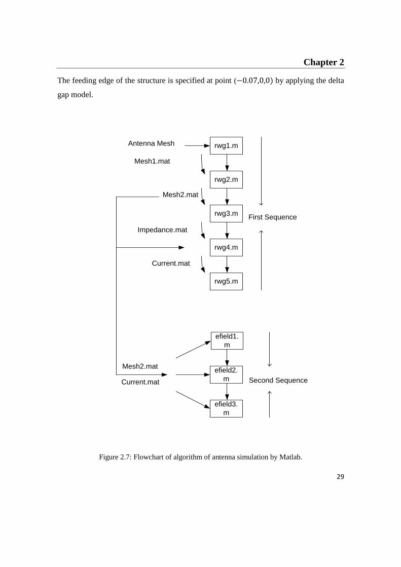
2.6 Code Sequence
The source code in the Matlab directory is divided into two sequences; the first
sequence includes the Matlab scripts rwg.m; the second one includes the Matlab codes
efield.m. Fig 2.7 shows the flowchart of algorithm which determines the process of
simulation by Matlab.
At the first step, the antenna structure is modeled analytically; then Delaunay
triangulation is applied to the structure by using Matlab function Delaunay. The script
rwg1.m and rwg2.m create RWG edge elements in order to compute the impedance
matrix in the Matlab script rwg3.m. Calculation of the input impedance and radiation
resistance are done in the script rwg4.m by determining excitation voltage. It is worth
noting, the source of the induced current could be either the voltage source with 1 𝑣 𝑚
magnitude and zero phase or an incident electromagnetic wave with 1 𝑣 𝑚 electric
field. The final script (rwg5.m) of the first sequence is devoted to visualize the surface
current distribution of the antenna; as shown in Fig 2.8.
After the first code sequence is complete, scripts efield1.m, efield2.m, and efield3.m
provide radiation signal at a point in the free space, radiation patterns of the antenna
including 3D patterns, and the antenna gain. It is noticeable that the files with mat suffix
(in Fig 2.7) are applied to save the information of each script; and using those
information in the next script.
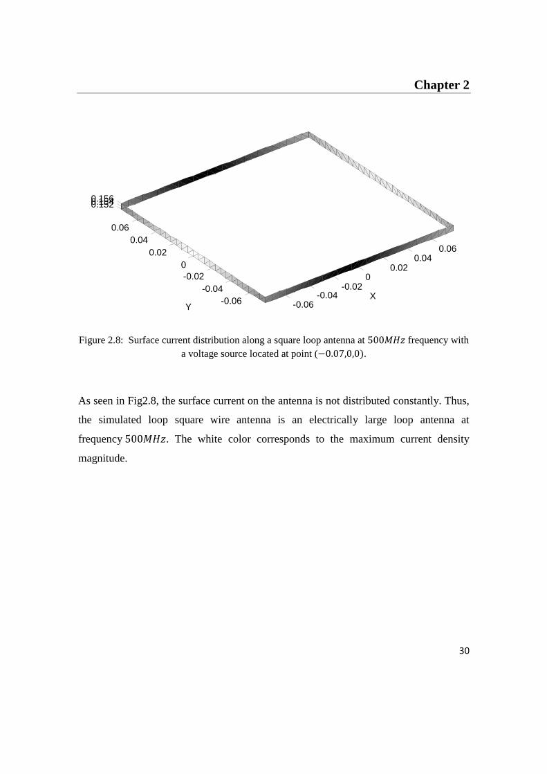
2.7 Electrically Large Loop Antenna
In this section, a square loop wire antenna with the length 𝑙 = 154𝑚𝑚 and the cross-
sectional radius 𝑟𝑤 = 1.1421 𝑚𝑚 at frequency 500𝑀𝐻𝑧 are created and the surface
current distribution along the antenna is visualized. The loop contains 325 triangles.
Page 38
Chapter 2
29
The feeding edge of the structure is specified at point (−0.07,0,0) by applying the delta
gap model.
rwg1.m
rwg4.m
rwg2.m
rwg5.m
rwg3.m
efield3.
m
efield1.
m
efield2.
m
Antenna Mesh
Mesh1.mat
Mesh2.mat
Impedance.mat
Current.mat
Mesh2.mat
Current.mat
First Sequence
Second Sequence
Figure 2.7: Flowchart of algorithm of antenna simulation by Matlab.
Page 39
Chapter 2
30
Figure 2.8: Surface current distribution along a square loop antenna at 500𝑀𝐻𝑧 frequency with
a voltage source located at point (−0.07,0,0).
As seen in Fig2.8, the surface current on the antenna is not distributed constantly. Thus,
the simulated loop square wire antenna is an electrically large loop antenna at
frequency 500𝑀𝐻𝑧. The white color corresponds to the maximum current density
magnitude.
-0.06 -0.04
-0.02 0
0.02 0.04
0.06
-0.06 -0.04
-0.02 0
0.02 0.04
0.06
0.152 0.154 0.156
X Y
Page 40
Chapter 3
31
Chapter 3
Optimization Method
3.1 Introduction
In recent years several evolutionary algorithms have been developed for optimization of
every type of electromagnetic problems. The general goal of the optimization is to find
a solution that represents the global maximum or minimum of a fitness function.
Electromagnetic optimization problems generally contains a large number of
parameters; these parameters can be either continuous, discrete, or both, and often
include constraints in allowable values. In addition, the solution domain of
electromagnetic optimization problems often has non differentiable and discontinuous
regions, and often utilizes approximations or models of the true electromagnetic
phenomena to conserve computational resources.
Global search methods present two competing goals, exploration and exploitation:
exploration is important to ensure that every part of the solution domain is searched
enough to provide a reliable estimate of the global optimum; exploitation, instead, is
also important to concentrate the search effort around the best solutions found so far by
searching their neighborhoods in order to reach better solutions. Often global search
methods are used together with other local search algorithm in order to improve
efficiency and accuracy of the searching process [31].
The evolutionary computation algorithms (EA) are stochastic optimization methods that
emulate biologic processes or natural phenomena. The capability of finding a global
Page 41
Chapter 3
32
optimum without being trapped in local optima, and the possibility of well face
nonlinear and discontinuous problems with great numbers of variables, are some
advantages of these techniques. Besides these methods do not needs to compute any
derivatives in order to optimize the objective function and this fact allows managing
more complex fitness function.
Moreover, in contrast with traditional searching methods, EAs do not depend strongly
on the starting point. Often a bad choice of the initial values can slow down the
convergence of the entire process; or even drive the convergence towards a wrong
solution (e.g. towards a local instead a global maximum or minimum). Although, these
algorithms have strong stochastic basis, but they need a lot of iterations to get a
significant result, in particular when the optimization problem has a big number of
unknowns.
Among the main evolutionary optimization approaches it is worth mentioning the
Genetic Algorithm (GA) and the Particle Swarm Optimization (PSO).
Msot of the times, PSO have faster convergence rate than GA early in the run, but they
are often outperformed by GA for long simulation runs, or when the number of
unknowns increases. This is due to the different types of search, adopted by the two
algorithms.
The new hybrid technique here proposed is called Genetical Swarm Optimization,
consists in a strong co-operation of GA and PSO, since it maintains the integration of
the two techniques for the entire run of simulation. In fact, in each iteration, some of the
individuals are substituted by new generated ones by means of GA, while the remaining
part is the same of the previous generation but moved on the solution space by PSO.
Doing so, the problem of premature convergence of the best individuals of the
population to a local optimum, one of the most known drawbacks found in tests of
hybrid global-local strategies, has been cancelled.
Page 42
Chapter 3
33
The effectiveness of the proposed procedure has been validated with different
electromagnetism problems, showing a good behaviour in particular for the
optimization of large-domain functions.
3.2 Genetic Algorithm
Genetic Algorithms simulate the natural evolution, in terms of survival of the fittest,
adopting pseudo-biological operators such as selection, crossover and mutation [32, 33].
In GA, the set of parameters that characterizes a specific problem is called an individual
or a chromosome and is composed of a list of genes. Each gene contains the parameter
itself or a suitable encoding of them. Each individual therefore represents a point in the
search space, and hence a possible solution to the problem. For each individual of the
population a fitness function is therefore evaluated, resulting in a score assigned to the
individual. Based on this fitness score, a new population is generated iteratively with
each successive population referred to as a generation. The GAs use three basic
operators (selection, crossover, and mutation) to manipulate the genetic composition of
a population. Selection is the process by which the most highly rated individuals in the
current generation are chosen to be involved as “parents” in the creation of a new
generation. The crossover operator produces two new individuals (i.e. candidate
solutions) by recombining the information from two parents. Genetic Algorithms are
very efficient at exploring the entire search space, but are relatively poor in finding the
precise local optimal solution in the region in which the algorithm converges. Many
efforts on the enhancement of traditional GAs have been proposed, by modifying the
structure of the population or the role that an individual plays in it; the Genetic
Algorithm developed for this application uses real encoded genes, since for high
number of variables they result in faster than binary ones in convergence towards the
maximum value.
Moreover, several additional operators have been developed for GA in order to get a
faster convergence rate; Hybrid GAs, in order to solve the previous problem, use local
Page 43
Chapter 3
34
improvement procedures as a part of the evaluation of the individuals of the population:
these procedures complement the global search strategy of the GA. Evidently, each
model is not optimal for all problems for many reasons. One of the most known
drawbacks that were found during tests of hybrid GA is the problem of premature
convergence of the best individuals of the population towards a local optimum.
3.3 Particle Swarm Optimization
The PSO has been introduced in the middle of 90’s [34, 35, 36] and it is based on
a”social interaction” metaphor in which the parameter space is searched by controlling
the trajectories of a set of particles according to a swarm- or flock-like set of rules. The
position of each particle is used to compute the value of the function to be optimized.
Individual particles are then attracted, with a stochastic-varying strength, by both the
position of their best past performance and the position of the global best past
performance of the whole swarm.
PSO is akin to the other stochastic methods performing a global search in the parameter
space without getting trapped in local minima. In the recent years the interest for its
application to electromagnetic problems has been rapidly increasing [37, 38, 39], and
several papers have been published comparing it with other optimization techniques,
mainly with GA [40, 41, 42, 43].
3.3.1 Traditional PSO Implementation
Particle Swarm Optimization (PSO) is one of the more recently developed evolutionary
techniques; it is based on a suitable model of social interaction between independent
agents (particles) and it uses social knowledge in order to find the global maximum or
minimum of a generic function [35]. While for the GA, as shown in section 3.2, the
improvement in the population fitness is assured by pseudo-biological operators, such as
selection, crossover and mutation, the main PSO operator is the velocity update that
Page 44
Chapter 3
35
takes into account the best position explored during the iterations, resulting in a
migration of the swarm towards the global optimum.
In the PSO the so called swarm intelligence (i.e. the experience accumulated during the
evolution) is used to search the parameter space by controlling the trajectories of a set of
particles according to a swarm-like set of rules [37, 38].
In particular, the position of each particle is used to compute the value of the function to
be optimized. Consequently every position is a particular solution of the optimization
problem. Individual particles traverse the problem hyperspace and are attracted by both
the position of their best past performance and the position of the global best
performance of the whole swarm. Particles are moved in the domain of the problem
with variable speeds and every position they reach represents a particular configuration
of the variables set, which is then evaluated in order to get a score.
At each step the position of each swarm particle corresponds to one potential “optimal”
solution for the problem, therefore the value of the function that mathematically models
the problem, the fitness or cost function, is evaluated for all these possible solutions and
the one that gives the best cost value.
As GA, the standard PSO algorithm is therefore an iterative procedure in which a set
of 𝑖 = 1. . , ,𝑁𝑝 particles, or agents, are characterized by their position Xi and velocity
Vi with which they move in the M-dimensional space domain 𝐷 of a cost function
𝑓(𝑋). A full treatment of the method can be found in [36] but for sake of clarity and
uniformity of notation it is briefly summarized in the following. At the beginning
positions and velocities have completely random values 𝑋𝑖(0)
and 𝑉𝑖(0)
, then they are
updated iteratively according to the rules:
𝑽𝒊𝒌+𝟏 = 𝝎𝒌𝑽𝒊
𝒌 + 𝝓𝜼𝟏 𝑷𝒊 − 𝑿𝒊𝒌 + 𝝓𝜼𝟐(𝑮 − 𝑿𝒊
𝒌) (3.1)
𝑿𝒊𝒌+𝟏 = 𝑿𝒊
𝒌 + 𝑽𝒊𝒌+𝟏 (3.2)
Page 45
Chapter 3
36
being 𝑃𝑖 the best position ever attained by particle 𝑖 itself (personal knowledge) and G
the best position ever attained by the particle swarm (social knowledge); 𝜔𝑘 =
𝜔0𝑒−𝛼𝑘 + 𝜔1 is a friction factor slowing down particles, 𝜂1 and 𝜂2 are positive
parameters tuning the pulls towards the personal and global best positions and 𝜙 is a
random number of uniform distribution in the [0,1] range. Please note that, if 𝜙 appears
more than once in a given formula it is assumed to have different values each time.
The presence of random weights in the pull terms generated by the particle’s best
position 𝑃𝑖 and the global swarm best position 𝐺 causes wide oscillations and a random
search in the entire parameter space. Such oscillations are precious whereas they
broaden the search of each particle but they have some drawbacks since they can
produce continuous oscillation around the optimal point. Such oscillation can be
dampened, and so the convergence enhanced, via an effective use of the 𝜔 parameter.
Having a friction factor which is a function of 𝑘 was suggested in [44]. Starting the
optimization process with a high value for 𝑘 and reducing it as 𝑘 increases encourage
the particles to explore the whole space domain in the beginning, in search of the global
minimum, and then allow them to better investigate the region in which this minimum is
supposed to be located.
An important aspect connected with the efficiency of the PSO is the way in which the
particles moving towards the border of the solution space are handled; in [42] three
different solutions are proposed: the first one consists in setting to zero the velocity of
the particles arriving at the domain boundary, the second one models the boundaries as
perfect reflecting surfaces, so that the particles impinging on them are reflected back in
the solution space; finally the third one allows the particles to fly out from the solution
space, without evaluating the cost function any more, until the particle eventually gets
back in the domain. In this work the second technique has been adopted, since
preliminary tests seem to suggest that this is the one guaranteeing the faster
convergence.
Page 46
Chapter 3
37
If the iterative process is not yet arrived at the end (i.e. if the cost function has not yet
reached the fixed threshold value or if the number of iterations does not equals the
maximum allowed) a new step is performed: particles move from their position
according to a swarm- or flock-like set of rules, being attracted, with a stochastic-
varying strength, by both the position of their best past performance and the position of
the global best past performance of the whole swarm. Note that the PSO completely
differs from the typical GA based evolutionary algorithms since it does not implement
any selection or mutation of individuals, but particles adapt themselves to the
geometrical characteristics of the solution space they are moving in.
3.3.2 Some Consideration on PS
The PSO is gaining a big popularity, especially because of its simplicity in
implementation, its robustness and its “optimization capability” for both single
objective and multi-objective problems. PSO proved to be in all considered cases at
least comparable, and often superior, to its most famous competitor, the GA [43, 45].
Besides the easiness of the implementation, the PSO presents the advantage of being
well suited for optimization problems with both discrete and continuous parameters, and
for parallel computing implementation [39, 46].
All these features make the PSO particularly appealing and attracted the interest of the
electromagnetic community in the last years [42, 47]. However, the use of such a
technique, requiring the evaluation of the cost function thousands of times needs
particular care for electromagnetic problems, in which the cost function is often very
computationally expensive. Moreover, there is some application in which PSO is by
outperformed by GA [43]. For this reason, the development of new versions of the PSO
algorithm with enhanced properties is a challenging issue.
Page 47
Chapter 3
38
3.4 The Class of Meta-Swarm Algorithm
Recently, the Particle Swarm Optimization (PSO) method has been successfully applied
to different electromagnetic optimization problems. Because of the complexity of this
kind of problems, the associated cost function is in general computationally expensive.
A rapid convergence of the optimization algorithm is hence required to attain results in
short time.
In this section some new PSO based techniques, aimed to improve the performances of
the standard PSO with a negligible overhead in the algorithm complexity and
computational cost are presented. All of them will exploit multiple interacting swarms.
In the literature, the use of more than one swarm or PSO is very sporadic, and, to the
author best knowledge, previously completely absent in conjunction with
electromagnetic problems. In [48] a division of the population in cluster is proposed.
Contrarily to what is done here, in [48] the particles belonging to a cluster are chosen
according to a ”minimum distance” criterion, and the equations that manage the
evolution of the single particle are modified, substituting its personal and/or the global
bests with those of the center of the cluster the particle belong to. In this way, however,
the complexity of the algorithm increases since the particles division into clusters must
be performed and managed. In [49] two separate PSOs are used to optimize a two-
objective problem: each PSO focus on one aspect of the problem and they interact
through the cost function. Finally, in [50] the Cooperative Particle Swarm (CPSO)
method is introduced. This technique splits the domain in subspaces, each searched by a
swarm, hence requiring additional functions to reconstruct the point where the cost
function is to be evaluated and a more complex way, with respect to conventional PSO,
to handle and store personal and global bests.
The most performing CPSO-𝐻𝑘 (H stands for Hybrid, k is the subspace dimension [50])
algorithms relies on the co-evolution of a CPSO and a PSO with exchange of
information between the two, leading to an even more complex algorithm. On the other
Page 48
Chapter 3
39
hand, the algorithms here presented exhibit just one or two terms to be summed to the
velocity update function, and no other additional complexity.
3.4.1 Undifferentiated Meta-Swarm
Here three variations over the standard PSO algorithm are described. All of them use
multiple swarms to enhance the capabilities of global search, but adopt different simple
rules for describing the interactions among them; therefore the overhead to the
traditional implementation is negligible.
The implementation here proposed is similar but simpler than those of Cooperative
Particle Swarm (CPSO) methods [51,52]. These latter splits the domain in subspaces,
each searched by a swarm, hence requiring additional functions to reconstruct the point
where the cost function is to be evaluated and a more complex way, with respect to
conventional PSO, to handle and store personal and global bests.
Figure3.1: Undifferentiated Meta-Swarm basic layout. Forces over a generic particle are: (a)
pull toward personal best𝑃1,𝑗 ; (b) pull toward swarm best 𝑆1; (c) pull toward global best G
(belonging to swarm 2); (d) repulsion from the other swarm’s barycentre 𝐵2.
Page 49
Chapter 3
40
Meta PSO
Meta PSO (MPSO) is the most straightforward of the methods here presented and
simply consists in using more than a single swarm. Particles are now characterized by
two indexes: an index 𝑗 = 1, . . . ,𝑁𝑠 defining the swarm they belong to and an index
𝑖 = 1, . . . ,𝑁𝑝𝑗 within the swarm. For sake of simplicity in the following all swarms
will be considered as having the same number of particles 𝑁𝑝 = 𝑁𝑝𝑗 ∀𝑗 =
1, . . . ,𝑁𝑠. The MPSO velocity update rule is:
𝑽𝒋,𝒊𝒌+𝟏 = 𝝎𝒌𝑽𝒋,𝒊
𝒌 + 𝝓𝜼𝟏 𝑷𝒋,𝒊 − 𝑿𝒋.𝒊𝒌 + 𝝓𝜼𝟑 𝑺𝒋 − 𝑿𝒋,𝒊
𝒌 + 𝝓𝜼𝟐(𝑮 − 𝑿𝒋,𝒊𝒌 ) (3.3)
where 𝑃𝑗 ,𝑖 is the particle personal best position, 𝑆𝑗 is the global best position of swarm
𝑗 (swarm social knowledge) and 𝐺 is the global best position of all swarms (racial
knowledge), while the other symbols have the same meaning as in (3.1).
Position update and boundary handling are the same as in standard PSO with just one
more index.
Modified Meta PSO
As an enhancement to MPSO aimed at keeping swarms apart from each other, and
hence widening the global search, an inter-swarm repulsion is introduced and a
Modified 𝑀𝑃𝑆𝑂 (𝑀²𝑃𝑆𝑂) produced. The velocity update rule becomes:
𝑽𝒋,𝒊𝒌+𝟏 = 𝝎𝒌𝑽𝒋,𝒊
𝒌 + 𝝓𝜼𝟏 𝑷𝒋,𝒊 − 𝑿𝒋.𝒊𝒌 + 𝝓𝜼𝟑 𝑺𝒋 − 𝑿𝒋,𝒊
𝒌 + 𝝓𝜼𝟐 𝑮 − 𝑿𝒋,𝒊𝒌
− 𝝓𝝃𝑩𝒔𝒌−𝑿𝒋,𝒊
𝒌
∣𝑩𝒔𝒌−𝑿𝒋,𝒊
𝒌 ∣𝜸𝒔≠𝒋 (3.4)
Page 50
Chapter 3
41
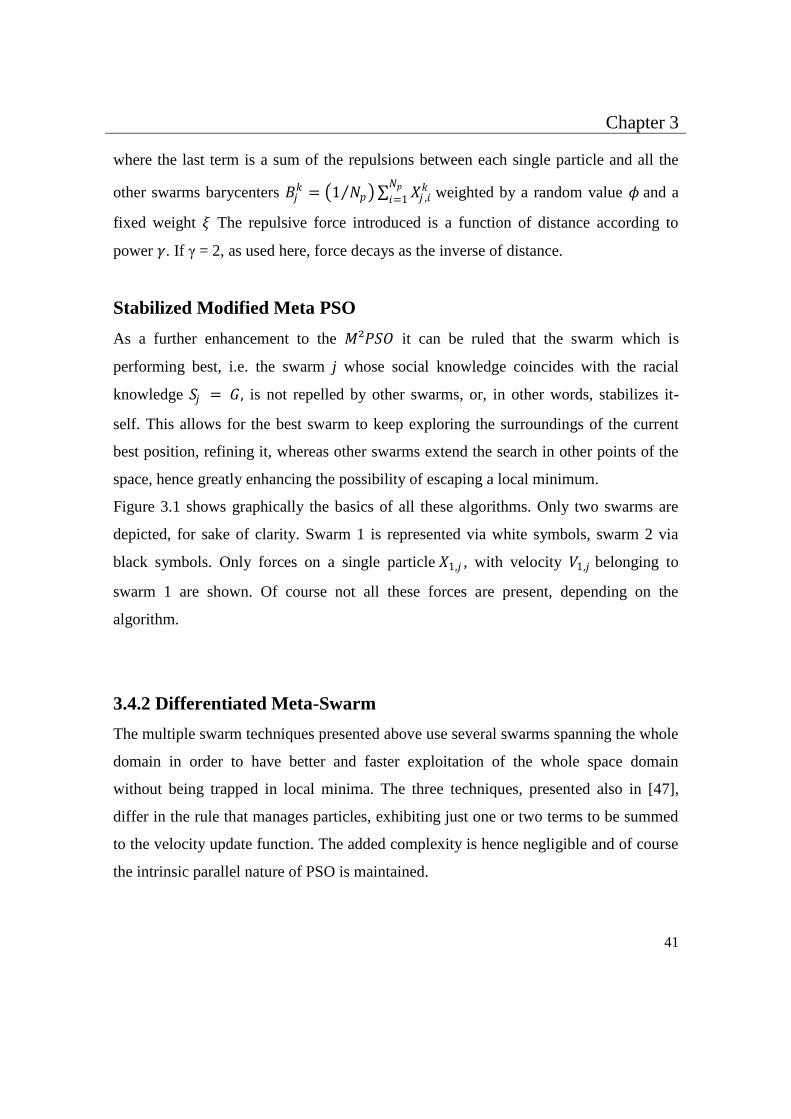
where the last term is a sum of the repulsions between each single particle and all the
other swarms barycenters 𝐵𝑗𝑘 = 1 𝑁𝑝 𝑋𝑗 ,𝑖
𝑘𝑁𝑝𝑖=1
weighted by a random value 𝜙 and a
fixed weight 𝜉 The repulsive force introduced is a function of distance according to
power 𝛾. If γ = 2, as used here, force decays as the inverse of distance.
Stabilized Modified Meta PSO
As a further enhancement to the 𝑀²𝑃𝑆𝑂 it can be ruled that the swarm which is
performing best, i.e. the swarm j whose social knowledge coincides with the racial
knowledge 𝑆𝑗 = 𝐺, is not repelled by other swarms, or, in other words, stabilizes it-
self. This allows for the best swarm to keep exploring the surroundings of the current
best position, refining it, whereas other swarms extend the search in other points of the
space, hence greatly enhancing the possibility of escaping a local minimum.
Figure 3.1 shows graphically the basics of all these algorithms. Only two swarms are
depicted, for sake of clarity. Swarm 1 is represented via white symbols, swarm 2 via
black symbols. Only forces on a single particle 𝑋1,𝑗 , with velocity 𝑉1,𝑗 belonging to
swarm 1 are shown. Of course not all these forces are present, depending on the
algorithm.
3.4.2 Differentiated Meta-Swarm
The multiple swarm techniques presented above use several swarms spanning the whole
domain in order to have better and faster exploitation of the whole space domain
without being trapped in local minima. The three techniques, presented also in [47],
differ in the rule that manages particles, exhibiting just one or two terms to be summed
to the velocity update function. The added complexity is hence negligible and of course
the intrinsic parallel nature of PSO is maintained.
Page 51
Chapter 3
42
These three techniques will be identified in the following as Undifferentiated Meta
PSOs, the word Undifferentiated meaning that all the particles of all swarms obeys to
the same rules.
The simplest of these Meta PSOs is further modified here, and two other new schemes
have been obtained, named in the following Differentiated Meta PSOs, in which the
behavior of the particles within a swarm is managed with different rules.
Despite of their simplicity, both the Undifferentiated and the Differentiated Meta-PSO
work better than the standard PSO. The effectiveness of the Undifferentiated and
Differentiated Meta-PSO algorithm can also find a confirmation in the analysis on the
different possible social interaction models reported in [53], in which it is hypothesized
that tightly connected particle swarms, as in the standard PSO scheme, may not be so
good in finding the problem optimum, since they can be entrapped in local sub-optima,
while this risk is lower in case of moderately connected societies, as the proposed
schemes are.
As opposed to the Meta-Swarms presented in section 3.4.1, in which each agent was
equal to any other agent, in the Differentiated Meta-Swarm algorithms proposed here
below different velocity update laws holds on agent-by-agent bases. In particular both
the proposed algorithms are still based on a multi-swarm approach, but in each swarm a
particle is bestowed a special ’leader’ status. If the bee similitude often used for PSO
holds, we can think of this special particle of each swarm as the ’queen bee’.
It is worth noticing that two different flavors for each of the algorithms described above
can be implemented, one where the leader particle never changes, and these will be
referred to as Absolute Leader algorithm, and one where the leader particle can change
within a swarm, usually by setting as leader the particle exhibiting the best performance
(the one whose personal best coincides with the swarm’s best). This second family will
be indicated as Democratic Leader algorithms. In this work the Leader paradigm will be
applied only to the MPSO algorithm.
Page 52
Chapter 3
43
In principle it can be applied to any Meta PSO algorithm but preliminary analyses
showed that the MPSO is the one taking the larger benefit. The resulting algorithms will
be denoted as ALMPSO or DLMPSO (Absolute Leader Meta-PSO and Democratic
Leader Meta-PSO), respectively. In these algorithms the leaders behave indeed as the
agents of a MPSO, with an attraction towards the leader personal best (personal
knowledge) an attraction towards the swarm best (social knowledge) and an attraction
towards the global best of all leaders (racial knowledge). On the other hand all other
swarms agents obey to interactions which are confined within the swarm itself, that is,
they are not subject to racial knowledge. The updating rule for the velocity of the MPSO
algorithm [47] can therefore modify as
𝑽𝒋,𝒊𝒌+𝟏 = 𝝎𝒌𝑽𝒋,𝒊
𝒌 + 𝝓𝜼𝟏 𝑷𝒋,𝒊 − 𝑿𝒋.𝒊𝒌 + 𝝓𝜼𝟑 𝑺𝒋 − 𝑿𝒋,𝒊
𝒌 + 𝝓𝜼𝟐 𝑮 − 𝑿𝒋,𝒊𝒌 +
𝜹𝒋,𝒊
𝑳𝒋𝝓𝜼𝟐(𝑮− 𝑿𝒋,𝒊𝒌 ) (3.5)
while the updating rule for the position remains the same as in (3.2):
𝑿𝒋,𝒊𝒌+𝟏 = 𝑿𝒋,𝒊
𝒌 + 𝑽𝒋,𝒊𝒌+𝟏 (3.6)
In (3.5) 𝛿𝑖𝑗
𝐿𝑗is a function which value is 1 only if 𝑖 = 𝐿𝑗 , being 𝐿𝑗 the index denoting the
leader of swarm j, otherwise it is 0.
Equation (3.5) holds of course both for Absolute and Democratic algorithms. In the
former case the value of 𝐿𝑗 is chosen at the beginning and never changed (in this case it
is computationally simpler to consider 𝐿𝑗 = 1, ∀𝑗 = 1 . . . ,𝑁𝑠); whereas in the latter
case 𝐿𝑗 is updated at each time iteration 𝑘 by having 𝐿𝑗 pointing to that agent for
which 𝑃𝑗 ,𝑖 = 𝑆𝑗 . In both cases the algorithm complexity is not significantly different
than that of a MPSO.
Page 53
Chapter 3
44
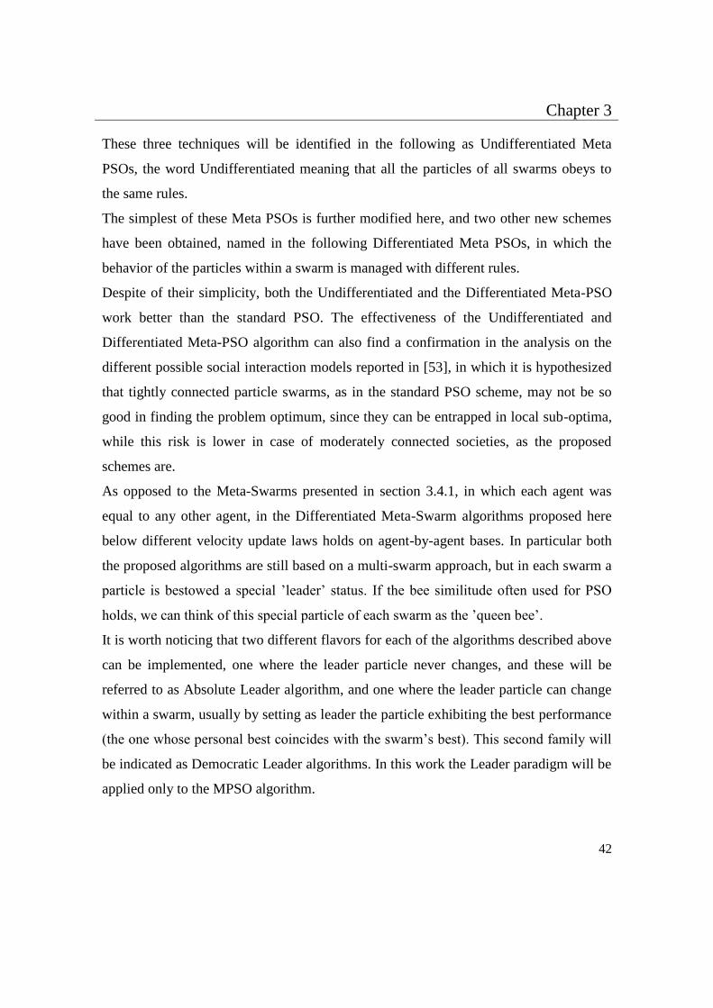
Fig3. 2 shows this algorithm graphically. As in the previous case only two swarms are
depicted, for sake of clarity. Swarm 1 is represented via white symbols, swarm 2 via
black symbols. The leader of each swarm is highlighted with an additional circle. The
swarm leader is subject to three forces, whereas each other particle in the swarm only to
two.
Figure3.2: Differentiated Meta-Swarm basic layout. Forces over the genetic particle are: (a)
pull toward personal best 𝑃1,𝑗 ; (b) pull toward swarm best 𝑆1. For what concerns the leader, he
is subjected also to (c) pull toward global best 𝐺 (belonging to swarm 2).
3.5 Genetical Swarm Optimization
Some comparisons of the performances of GA and PSO are present in literature [54],
underlining the reliability and convergence speed of both methods, but continuing in
keeping them separate.
Due to the different search method adopted by the two algorithms, the typical selection-
crossover-mutation approach versus the velocity update one, both the algorithms have
shown a good performance for some particular applications but not for other ones. For
example we noticed in our simulations that sometimes GA outperformed PSO, but
Page 54
Chapter 3
45
occasionally the opposite happened showing the typical application driven characteristic
of any single technique. In particular PSO seems to have faster convergence rate than
GA early in the run, but often it is outperformed by GA for long simulation runs, when
the last one finds a better solution.
Anyway, the population-based representation of the parameters that characterizes a
particular solution is the same for both the algorithms; therefore it is possible to
implement a hybrid technique in order to utilize the qualities and uniqueness of the two
algorithms.
Some attempts have been done in this direction, with good results, but with a weak
integration of the two strategies. Precisely, most of the times, one technique is used
mainly as a pre-optimizer for the initial population of the other technique. In [55], for
example, the authors test two different combinations of GA and PSO, using the results
of one algorithm as a starting point for the other (in both the orders) to optimize a
profiled corrugated horn antenna.
Another hybridization strategy is proposed in [56], where the upper-half of the best-
performing individuals in a population is regarded as elite and, before using GA
operators, it is first enhanced by means of PSO, instead of being reproduced directly to
the next generation.
The hybrid technique here proposed, called Genetical Swarm Optimization (GSO), and
consists in a strong co-operation of GA and PSO, since it maintains the integration of
the two techniques for the entire run. In fact, this kind of updating technique yields a
particular evolutionary process where individuals not only improve their score for
natural selection of the fitness or for good-knowledge sharing, but for both of them at
the same time.
In each iteration, the population is divided into two parts and they are evolved with the
two techniques respectively. They are then recombined in the updated population, that is
again divided randomly into two parts in the next iteration for another run of genetic or
particle swarm operators. Fig3. 3 and Fig3. 4 show the flowchart of the developed
Page 55
Chapter 3
46
algorithm, the idea that stands behind the algorithm and the way to mixing the two main
techniques, respectively.
The population update concept can be easily understood thinking that a part of the
individuals is substituted by new generated ones by means of GA, while the remaining
are the same of the previous generation but moved on the solution space by PSO.
Figure3. 3: The flow-chart of the GSO algorithm.
The driving parameter of GSO algorithm is the Hybridization Coefficient ℎ𝑐(𝑖); it
expresses the percentage of population that in each iteration is evolved with GA: so
ℎ𝑐(𝑖) = 0 means the procedure is a pure PSO (the whole population is processed
according to PSO operators), ℎ𝑐(𝑖) = 1 means pure GA (the whole population is
processed according to GA operators), Whereas, 0 < ℎ𝑐(𝑖) < 1 means that the
Random
population
Fitness
evaluation
of all
individuals
Splitting of
population
Selective
reproduction
Crossover
Mutation
Resulting
new
population
Velocity
updating
Calculation of
new positions
Personal and
global bests
updating
Stop?
no
yes Best
individuals
Start End
PSOPSOGAGA
Random
population
Fitness
evaluation
of all
individuals
Splitting of
population
Selective
reproduction
Crossover
Mutation
Resulting
new
population
Velocity
updating
Calculation of
new positions
Personal and
global bests
updating
Stop?
no
yes Best
individuals
Start End
PSOPSOGAGA
Page 56
Chapter 3
47
corresponding percentage of the population is developed by GA, while the rest with
PSO technique.
Figure3. 4: Splitting of the population in subgroups during the iterations.
3.5.1 The GSO Algorithm Class
The hc approach opens a wide spectrum of possible merging strategies between GA and
PSO, since the hc itself can be varied during the optimization run. In fact, the number of
individuals evolved by a particular procedure, in each iteration, can change according to
predefined variation rules of the hc parameter, in order to exploit a better convergence.
This feature essentially extends the GSO concept to stand as a class of hybrid
evolutionary algorithms.
For instance, a step variation of hc between 0 and 1 (or vice versa) occurring after half
the run, realizes an hybridization approach similar to the one used in [55], where the
population is initially evolved by PSO, then the resulting individuals, after about 50%
iterations, are evolved by GA (and vice versa).
The different rules of variation of ℎ𝑐(𝑖) during iterations identify several “flavours” in
the class of GSO algorithms, as shown in [57]: both traditional implementations of PSO
and GA can be obtained too, by keeping ℎ𝑐 𝑖 = 0 and ℎ𝑐 𝑖 = 1 for the entire run.
Page 57
Chapter 3
48
The best value of ℎ𝑐 𝑖 or its best variation rule for a given problem are hardly known a
priori. Therefore the two different adaptive rules were proposed, in order to combine in
the most effective way the properties of the GA and the PSO approaches also for
unknown problems.
The first one is the so-called Dynamical GSO, as referred in [57]; in this implementation
the ℎ𝑐 parameter is updated during iterations according to the following rule:
𝒇 𝒙 = 𝒉𝒄 𝒊 + 𝒗𝒆−𝝃
𝒊′
𝑵
𝒌, 𝑖𝑓𝚫𝒇 𝒊′ < 𝚫𝒇 (𝒊)
𝒉𝒄(𝒊), 𝑖𝑓𝚫𝒇 (𝒊′) ≥ 𝚫𝒇 (𝒊)
(3.7)
Where 𝑁 is the total number of iterations, 𝐾 is the number of individuals in the
population, 𝑖 ′ = 𝑖 + Δ𝑖, 𝑣 = ±1 (versus), 𝜉 = 2 (damping), and Δ𝑓 𝑖 ′ = 𝑓 𝑖 ′ − 𝑓 (𝑖);
here 𝑓 (𝑖 ′) is the best fitness value obtained after 𝑖 ′iterations and ∆𝑖 = 5.
The second implemented technique is the so-called self-Adaptative GSO that derives the
ℎ𝑐 updating rule from the traditional PSO technique: in fact, if we consider the value of
ℎ𝑐 𝑖 ′ in the 𝑖 ′ -th iteration, then we can call 𝑉ℎ𝑐(𝑖′) the variation between ℎ𝑐(𝑖 ′) and
ℎ𝑐(𝑖) and so we can write:
𝒉𝒄 𝒊′ = 𝒉𝒄 𝒊 + 𝑽𝒉𝒄(𝒊′) (3.8)
Therefore, the problem is simply to find the right velocity update to properly change
ℎ𝑐(𝑖) during the run; following the PSO similarity, we can define a personal best 𝑃ℎ𝑐
value that has been obtained during the run and therefore write:
𝑽𝒉𝒄 𝒊′ = 𝝎.𝑽𝒉𝒄 𝒊 + 𝝓.𝜼. (𝑷𝒉𝒄 − 𝒉𝒄 𝒊 ) (3.9)
Page 58
Chapter 3
49
Where 𝑃ℎ𝑐 is chosen analyzing the slope of the increasing of the fitness score during the
iterations, i.e. if in iteration 𝑖 the increment of fitness is higher than in the previous
history, then 𝑃ℎ𝑐 = ℎ𝑐(𝑖 ).
However, differently from the traditional expression for the velocity update of standard
PSO, in this case the problem is mono-dimensional and there is only one single agent,
therefore the personal best of 𝑃ℎ𝑐 is also the global best, and so the definition of (3.9) is
simpler than (3.1). It is worth noticing that this updating procedure can not take
advantage of the cooperation among several particles, therefore, to avoid stagnation in
sub-optimal values, a random mutation is added to the ℎ𝑐(𝑖) value when the slope of the
fitness curve and the velocity are equal to zero.
Preliminary analyses are here presented with respect to the other optimization
techniques dealing with classical optimization problems. The application of these tools
to the antennas developed for this work will be presented in the next chapter.
3.5.2 Preliminary Analysis
With the aim to validate the effectiveness of the developed technique, we used different
values of hc in order to discover the best hybridization parameter and to compare GSO
with pure PSO and GA, simply by setting ℎ𝑐 = 0 or ℎ𝑐 = 1.
A first comparison of the different performances has been made on a classical
optimization problem, i.e. finding the maximum of an N-dimensional 𝑠𝑖𝑛𝑐 function
given by the equation:
𝒇 𝑿 = 𝐬𝐢𝐧(𝒙𝒊−𝒙𝟎,𝒊)
(𝒙𝒊−𝒙𝟎,𝒊)
𝑵𝒊=𝟏 (3.10)
where N is the dimension of the domain, 1,0ix and ix i 3.0,0 .
Page 59
Chapter 3
50
To analyze the efficiency of the different approaches when the solution space dimension
increases, three different cases of growing complexity were chosen , thus considering N
= 5, 10 and 20.
The results reported in Fig3. 5-7 shows the fitness behaviour related to different hc
values for the sinc function for different problem dimensions. In additional, from
preliminary analyses it has been clear that the value of ℎ𝑐(𝑖) plays a role in affecting the
speed of convergence, for instance very good performances have been obtained for the
optimization of the sinc function by considering ℎ𝑐 𝑖 = 0.2,∀ 𝑖 for the N-dimensional
𝑠𝑖𝑛𝑐 function and it does not depend on the dimension of the problem. Furthermore, the
obtained best hc value (0.2) means that, for a big sized problem, the basic PSO can be
strongly improved by adding a small percentage of genetic operators on the population.
Figure3. 5: Final fitness for different hc values (5-D 𝑠𝑖𝑛𝑐 function optimization, average over
50 samples).
Page 60
Chapter 3
51
Moreover, while for a small number of unknown GSO performance is similar to GA
and PSO ones (Fig. 3.5), if the size of the problem increases (Fig. 3.6, 3.7), GSO
behaviour improves and outperforms GA and PSO during iterations.
Figure3. 6: Final fitness for different hc values (10-D sinc function optimization, average over
50 samples).
It is important to notice that the evaluation of the fitness function is the most relevant
time consuming task, while the computational overhead of the optimizer operators,
different for the considered techniques, is negligible. This is particularly true in
electromagnetic optimization. Therefore the larger the population, the longer is the
single iteration, since several evaluations of the fitness function must be performed to
complete the step. For this reason, the different techniques have been compared in terms
Page 61
Chapter 3
52
of performed fitness evaluations rather than iterations, in order to fairly compare the
different algorithms regardless of the number of individuals in the population.
Furturemore, as results reported in Fig3.8-10 show, it seems that the improvments
introduced by the hybridization are increasing with the dimention of the problem to be
Figure3. 7: Final fitness for different hc values (20-D sinc function optimization, average over
50 samples).
optimized: if we consider the optimization of the well-known 𝑁-dimensional sinc
function, for 𝑁 = 5 average performance of all the considered method (increasing GA
and PSO, for comparison) are almost the same , although the traditional methods
sometimes fails in finding the optimal value, as shown by the bar indicating the worst
performance (over 100 independent trials) in Fig3. 8. When 𝑁 = 10, the average
Page 62
Chapter 3
53
performances of GSO as slighty better than GA and significantly better than PSO
(Fig3.9), while, for 𝑁 = 20, the improvement introduced by the hybridization is not
negligible, since just the different GSO implementations are able to locate the optimal
value, as shown by the bar indicating the best performance in Fig3. 10, while, for the
considered number of iterations, neither GA nor PSO are able to get the optimal value in
100 trials and their average performance is lower than GSOs’one. Moreover, the best
performance is here obtained using ℎ𝑐 = 0.2, since this value has been found to be the
optimal for this kind of problem, but anyway the adaptive straegies are still better than
the traditional technique.
Figure3. 8: Final values of the sinc function optimization with N = 5 variables
obtained with different hybridization strategies (average results over 100 trials).
Page 63
Chapter 3
54
3.5.3 Performance Analysis
With the aim of validating the effectiveness of the developed technique for
electromagnetic applications, the author chose the optimization of a linear array of 100
elements. This application has been already considered in literature in order to compare
the performances of the different algorithms in the determination of the complex phased
array weights to best meet a specified far-field side-lobe requirement.
The antenna is a linear phased array of one hundred half-wavelength spaced radiators.
The far-field radiation pattern to be optimized is 𝐹.𝐹. (𝜃) = 𝐸.𝑃. (𝜃) ・ 𝐴.𝐹. (𝜃),
where
𝑨 ∙ 𝑭 𝜽 = 𝑨𝒏𝒆𝒋𝟐𝝅𝒏(𝒅 𝝀) 𝐬𝐢𝐧 𝜽 𝑵
𝒊=𝟏 (3.11)
is the array factor in which is the number of radiative elements, are the complex element
weights to be determined. The voltage element pattern, according to [54] is assumed to
be:
𝑬 ∙ 𝑷 ∙ (𝜽) = 𝒄𝒐𝒔𝟏.𝟐𝜽 (3.12)
The cost measure to be minimized is the arithmetic mean of the squares of the excess
far-field magnitude above the specified side-lobe level. The side-lobe mask is the same
used in [54] which include a 60 𝑑𝐵 notch on one side.
In the present work, the GA engine implemented in GSO uses real encoding of genes
with tournament selection; uniform crossover occurs with probability 𝑃𝑐𝑟𝑜𝑠𝑠 = 80%
while the random mutation rate is 𝑃𝑚𝑢𝑡 = 5%. For PSO we use 𝜙1 = 2, 𝜙2 = 2 and
𝜔 = 0.7 in equation (3.1). Each run has been conducted with a population of 10
individuals and stopped after 50 000 iterations.
Page 64
Chapter 3
55
Several hybridization techniques have been tested for the optimization of the linear
array: Fig3.11 and Table 3. 2 show the results of the best four procedures, after 400 000
fitness evaluations, as well as the average of 100 trials.
The effectiveness of GSO method emerges both for the static case (ℎ𝑐 = 0.2) and for
the self-adaptive case, that results a fast and reliable hybridization strategy.
This technique is exploiting the distinctive attributes of the two algorithms, results in a
general purpose tool that can represent a fast method for optimization of large domain
objective functions. This feature makes it suitable for application on a wide range of
electromagnetic problems.
Fig.ure3. 9: Final values of the sinc function optimization with N = 10 variables
obtained with different hybridization strategies (average results over 100 trials).
Page 65
Chapter 3
56
Figure3. 10: Final values of the sinc function optimization with N = 20 variables
obtained with different hybridization strategies (average results over 100 trials).
Table3. 1: results of the sinc function optimization for different problem dimensions and rules
of variation for the hc parameter during iterations: average final values over 100 independent
trails and, in parentheses, their standard deviation.
Page 66
Chapter 3
57
Figure 3.11: Performance comparison between different techniques for the linear
array optimization (100 trials).
Table 3.2: Linear Array Optimization.
Page 67
Chapter 4
58
Chapter 4
Design and Numerical Results
4.1 Introduction
In chapter two, we described the Method of Moment –Matlab Codes, which later in this
chapter will be employed to investigate the properties of the loop wire antenna under
analysis. Whereas, we devoted chapter three to explain two dominate evolutionary
optimization methods- Genetic Algorithm and Particle Swarm Optimization- and we
showed Particle Swarm Optimization in detail for electromagnetic problems. At the end
of the chapter three, Genetic Algorithm and Particle Swarm Optimization has been
merged in well cooperation to present a new evolutionary optimization method, is called
Genetical Swarm Optimization.
In this chapter, the proposed evolutionary optimization method (Genetic Swarm
Optimization) will be applied to optimize the square loop wire antenna by considering
fractal variation.
And then, the candidate antenna is analyzed by electromagnetic solver (MoM-Matlab
Code); automated design procedure is illustrated in Fig4.1. We should mention that, for
the first time, Kim and Jaggared [58] introduced the application of the fractal to the field
of antenna theory. At the final section of this chapter, we will simulate the structure
under analysis by commercial simulator such as FEKO-Lite [59] and compare those
with the obtained results by Matlab in order to check and verifying the reliability our
design.
Page 68
Chapter 4
59
Figure4.1: Illustration of design procedure.
4.2 Considered Geometry
In order to optimize antenna for wireless energy transfer, and to improve the wireless
link performances of WPT, preliminary analyses have been conducted on an equivalent
model based on two identical square loop wire antennas, as reported in Fig4.2, separated
by an air gap. The choice of such geometry is due to the need of reducing antenna
dimension [60].
The starting geometry is a square loop antenna. The following geometries are the results
of Genetical Swarm Optimization with respect to the fractal variation, as shown in Fig4.
3. The direction of the arrows, pointes in the output of Genetical Swarm Optimization
order.
Page 69
Chapter 4
60
Figure4. 2: A schematic of idea of the two identical antennas.
(a) (b)
(c) Optimized
Figure4. 3: Loop wire antenna shape and its optimization.
Page 70
Chapter 4
61
4.3 Simulation Analysis
Scattering Parameters
Scattering parameters or S-parameters are used to describe the behavior of a network at
high-frequency, where the network is complex and it is difficult to present the
characteristics of the network with lumped parameters. On other hand, S-parameters
make possible to treat a network as a “black box”; as shown in Fig4.4.
+ +
- -
Network
(Black Box)
I2I1
V1 V2
Figure4. 4: Two ports network.
We considered the “black box” contents two antennas in communication. The
transmitting power from antenna 1 and the receiving power by antenna 2 are defined in
term of S-parameters matrix as the following:
𝑺𝟏𝟏 𝑺𝟏𝟐
𝑺𝟐𝟏 𝑺𝟐𝟐 (4.1)
𝑆11 and 𝑆22 refer to the reflected power by antenna1 and 2, respectively. 𝑆12 and 𝑆21
represent the transferred power from antenna 1 to antenna 2 and vice versa. Hence, the
small value of 𝑆11 means, the most of the transmitting power has radiated in the free
Page 71
Chapter 4
62
space from antenna 1 and the less amount of the transmitting power has reflected at port
of the antenna 1. Whereas, the big value of 𝑆21 implies that the most of the delivered
power from the antenna 1 to the antenna 2 has been absorbed by antenna 2.
Therefore, if we would be able to redesign two antennas in communication with small
value for the reflection coefficient (𝑆11) and big value for the transmission coefficient
(𝑆21), it is worth saying that we increased performance between antennas.
S-parameters could be cast in terms of the terminal voltages and currents at two ports
network; shown in Fig4 .5:
𝑺𝟏𝟏 = 𝟏 − 𝒚𝟏𝟏 𝟏 + 𝒚𝟐𝟐 + 𝒁𝟎𝒚𝟏𝟐𝒚𝟐𝟏
∆ (𝟒. 𝟐)
𝑺𝟐𝟏 =−𝟐𝒚𝟐𝟏
∆ (𝟒.𝟑)
Where, 𝑍0 = 50
∆= 𝟏 + 𝒁𝟎𝒚𝟏𝟏 𝟏 + 𝒁𝟎𝒚𝟐𝟐 − 𝒁𝟎𝒚𝟏𝟐𝒚𝟐𝟏
𝒚𝟏𝟏 =𝑰𝟏𝑽𝟏
|𝑽𝟐=𝟎
𝒚𝟐𝟐 =𝑰𝟐𝑽𝟐
|𝑽𝟏=𝟎
𝒚𝟏𝟐 =𝑰𝟏𝑽𝟐
|𝑽𝟏=𝟎
𝒚𝟐𝟏 =𝑰𝟐𝑽𝟏
|𝑽𝟐=𝟎
Page 72
Chapter 4
63
Reciprocity Theory
The reciprocity theorem is utilized in simplifying the antenna theory, it is named base on
its application in the antenna theory. Strong Reciprocity Theorem allows deducing the
properties of receiving antennas from those of transmitting antennas and vice versa,
where receiving and transmitting antennas are identical. Week Reciprocity Theorem
allows interchanging in the performance of receiving and transmitting antennas, where
all the differences are in the construction of receiving and transmitting antennas (refer to
[61] in order to more understanding of week reciprocity theorem). In this study, we have
applied strong reciprocity theorem in order to simplifying our designed antennas.
Strong Reciprocity Theorem
Assume two identical antennas by a gap separation. A voltage source is placed at the
terminal port of the antenna I and the flowed current through the antenna, produces the
electromagnetic force 𝐸1. Antenna II is excited by the electromagnetic force 𝐸1 and a
current is induced through the antenna.
Strong reciprocity theorem states that if this time, the voltage source is applied at the
terminal port of antenna II, the induced current through antenna I, while antenna I is
exposed to the radiated electromagnetic force 𝐸2 from antenna II, is equal to the induced
current through antenna II by the radiated electromagnetic force 𝐸1 from antenna I.
Thus, S-parameters of a network with strong reciprocity and symmetric characteristic
could be simplified as:
𝑺𝟐𝟏 = 𝑺𝟏𝟐
𝑺𝟏𝟏 = 𝑺𝟐𝟐
4.3.1 Antenna Optimization Procedure
The procedure of optimization and design is described as the following:
Page 73
Chapter 4
64
Each candidate antenna (the output of Genetical Swarm Optimization) is simulated by
Matlab in the frequency rang 450𝑀𝐻𝑧 − 600𝑀𝐻𝑧. We are interested in this range
frequency (Low Ultra High Frequency) due to being ideal for a whole range of
applications indoors/outdoors and appearing perpetually in urban areas.
Matlab simulation is interactively called by the presented optimization procedure, in
order to evaluate the coupling performances of the proposed antenna geometrics, as
shown in Fig4.3.
The aim of the analysis was to design the geometry in order to maximize the coupling
versus the displacement.
The data interface between optimization algorithm and numerical modeler is managed by
a built-in function called “fitness function”. The fitness function (FF) decodes the
information provided by GSO into geometrical dimensions to assign to the antenna
design; afterwards, FF analyses the new configuration and then it evaluates the
feasibility, the 𝑆11and 𝑆21 of parameters of the wireless system.
In order to maximize the energy transfer it is desirable to have antenna matched in the
frequency band of interest, and minimizing 𝑆11that is the return loss at port 1. Moreover,
it is necessary to maximize the coupling performance 𝑆21 .
To reach out these different objectives, we chose a multi-objective approach called ε-
constrained method [62] by adopting thresholds for the fitness function in order to
identify different phases into fitness score evaluation: In the first stage, fitness score
value ƒ is then defined as:
ƒ═ − 𝟓𝟎 (𝒖𝒏𝒕𝒊𝒍 𝒈𝒆𝒐𝒎𝒆𝒕𝒓𝒚 𝒊𝒔 𝒇𝒆𝒂𝒔𝒊𝒃𝒍𝒆)
Page 74
Chapter 4
65
Load= 50
Voltage Source= 1V
d
Receiving
antenna
Transmitting
antenna
L
Figure4. 5: case study analyzed with Matlab.
In order to penalize unfeasible solutions; when geometrical feasibility is obtained, ƒ is
computed as:
ƒ═ − 𝟑𝟎 − 𝑺𝟏𝟏 (𝒊𝒇 𝑺𝟏𝟏 > −10)
To minimize, return loss at the considered working frequency. Finally, when return loss
has reached the desired value:
ƒ═ 𝑺𝟐𝟏 (𝒊𝒇 𝑺𝟏𝟏 < −10)
In order to, maximize antenna matching at the considered working frequency.
Page 75
Chapter 4
66
Here, the optimization procedure considers a population of 10 candidate solutions per
iteration and it runs for 500 iterations, thus leading to 5000 cost function calls. Self-
adaptive hc is considered to maximize the GSO performances, as reported in [63].
A sample evolution of fitness value is reported in Figure4. 6; where the stage 2 and 3 are
highlighted. Moreover, in the same figure the hc value during iterations is reported,
showing that, in this particular case, self-adaptive GSO goes towards an almost exclusive
application of PSO operators. For each configuration mentioned in 4.2 section, 𝑆11 is
plotted, versus 𝑆21 to observe the reflection of the optimization procedure in the
antenna size and the antenna matched. As presented in Fig4. 7, the optimized antenna has
the best matching and size.
As well as, the scattering parameters and the dimensions of the considered geometries in
section 4.2 are shown in Fig4 .8, Fig4. 9 and Fig4. 10, respectively.
As been observed in Fig4. 8 and Fig4. 9, the smallest value of 𝑆11and the greatest value
of 𝑆21 are belonged to the optimized antenna; moreover, the size of antenna is minimized
by the optimized antenna. It means the optimized candidate met the all requirements for
having robustness coupling between antennas.
In wireless power transfer technology, the power efficiency is a key parameter. The
power gain or efficiency of the analyzed geometrics can be expressed as follows:
𝜼 = 𝑷𝒐𝒘𝒆𝒓 𝒅𝒆𝒍𝒊𝒗𝒆𝒓𝒆𝒅 𝒕𝒐 𝒕𝒉𝒆 𝒍𝒐𝒂𝒅
𝑷𝒐𝒘𝒆𝒓 𝒇𝒓𝒐𝒎 𝒔𝒐𝒖𝒓𝒄𝒆=
∣ 𝑺𝟐𝟏 ∣ ²
𝟏−∣ 𝑺𝟏𝟏 ∣ ²
And the efficiency of each candidate is plotted in Fig4. 11. The optimized candidate
reached the highest efficiency, as shown in Fig4. 11. The candidate (b) also has the
good efficiency as the optimized candidate; as you have observed in Fig4.7, the
candidate (b) is not however well-matched and sized to compare with the optimized
Page 76
Chapter 4
67
configuration. The design procedure is well suited in order to increase energy efficiency
and the robustness of the coupling, with the aim of improving the transmission power
wirelessly.
Figure4. 6: Evolution of fitness score and hc values during iterations.
4.4 Distance and Power Gain
Parameter d in Fig4. 5 indicates the distance between the origin point of the transmitting
antenna and the receiving antenna; the parameter d is fix in pervious simulations and
models. The distance d between two candidate antennas was considered equal to the
length of the one side of the antenna; for instance, the parameter d in Fig4. 5 equals to
the length of the side of the optimized antenna L= 91mm.
0 50 100 150 200 250 300 350 400 450 500
-20
-10
0
Fitness max Value
Iterations
0 50 100 150 200 250 300 350 400 450 500 0
0.5
1 hc value during the run
Iterations
Page 77
Chapter 4
68
4.5 5 5.5 6
x 10 8
-30
-25
-20
-15
-10
-5
0 Configuration (b)
Frequency, Hz
S 1 1
S 2 1
Matching: bad Size: Improved
4.5 4.6 4.7 4.8 4.9 5 5.1 5.2 5.3 5.4
x 10 8
-25
-20
-15
-10
-5
0
Frequency, Hz
S 1 1
S 2 1
Configuration (a)
Matching: good Size: bad
S-Parameters, dB
S-Parameters, dB
Page 78
Chapter 4
69
Figure4. 7: The matching antenna for each geometry.
4.5 5 5.5 6
x 10 8
-35
-30
-25
-20
-15
-10
-5
0
5
Frequency, Hz
Optimized Configuration
S 1 1
S 2 1
Matching: best Size: best
4.5 5 5.5 6
x 10 8
-35
-30
-25
-20
-15
-10
-5
0 Configuration (c)
Frequency, Hz
S 1 1
S 2 1
Matching: bad Size: improved
S-Parameters, dB
S-Parameters, dB
S-Parameters, dB
Page 79
Chapter 4
70
Figure4. 8: Return loss comparison of each configuration.
Figure4. 9: Coupling performance of each configuration.
4.5 5 5.5 6
x 10 8
-35
-30
-25
-20
-15
-10
-5
0
Frequency, Hz
𝑆21 , dB
Optimized Configuration
Configuration (a) Configuration (b)
Configuration (c)
4.5 5 5.5 6
x 10 8
-25
-20
-15
-10
-5
0
5
Frequency, Hz
𝑆11, dB
Optimized Configuration
Configuration (a) Configuration (b)
Configuration (c)
Page 80
Chapter 4
71
Figure4. 10: Size comparison of analyzed geometrics.
Figure4. 11: The power efficiency of the considered configurations.
4.5 5 5.5 6
x 10 8
-100
-50
0
50
Frequency, Hz
Optimized Configuration
Configuration (a)
Configuration (b)
Configuration (c)
(a) (b) (c) opt.(c) 0
50
100
150
200
250
[mm]
Antenna dimension
Side Diameter
Power Efficiency, %
Page 81
Chapter 4
72
As mentioned in Resonance Inductive Coupling section of chapter one, the coupling
performance of the antennas would decrease by increasing the distance between them.
Thus, improving the power gain over the longer distance, gives possibility to extend the
applications of this technology.
In this section, we supposed that the distance d is a variable parameter. The power gain
or efficiency is computed and plotted for several different values of the d in order to
investigate the impact of the longer distance on our optimized model, see Fig4. 12. At
the end, the worse case (the model with the longest d) is compared with the
configuration (a) with 𝐿 = 154 𝑚𝑚 and the same d as the worse case, shown in Fig4.
13.
As been seen in Fig4. 12, increasing the separated gap of antennas cause the decreasing
of the antenna coupling. However, the worse case (𝑑 = 250 𝑚𝑚) of the optimized
antenna has still higher efficiency than two square loop antennas with the same
separated gap and longer length; as presented in Fig4. 13. This means that we are
managed to optimize the simple square loop antenna structure, which is able to deliver
more power over longer distance.
4.5 Frequency Analyzing
The loop antenna is named the electrically large antenna, when the perimeter of the
loop antenna is greater than 𝜆10 .
𝑷𝒍𝒐𝒐𝒑 ≫ 𝝀𝟏𝟎 (4.4)
Large loop antenna usually has either a circular or square shape. Both circular and
square loops are usually operated near the first resonance point, which occurs for a
perimeter of slightly greater than one wavelength [64].
Page 82
Chapter 4
73
Figure4. 12: the efficiency of transferred power in each distance.
Figure4. 13: Comparison the worse case and two loop square antennas.
4.5 5 5.5 6
x 10 8
0
1
2
3
4
5
6
7
8
Frequency, Hz
Power
Efficiency, %
Loop square antenna
The analyzed antenna
d= 250 mm in both case
4.5 5 5.5 6
x 10 8
0
10
20
30
40
50
60
70
80
Frequency, Hz
250mm
125mm
100mm
83mm
50mm Power
Efficiency,
%
Page 83
Chapter 4
74
𝑷𝒍𝒐𝒐𝒑 > 𝝀𝒇𝒓 (4.5)
Where, 𝜆𝑓𝑟 is the wavelength at the resonance frequency.
𝝀𝒇𝒓=
𝟑∗𝟏𝟎𝟖
𝒇𝒓 (4.6)
The following table I reports the perimeter and one wavelength at the resonance
frequency for the candidate antennas. The configuration (a) and the optimized antenna
are only which meet the equation (4.5). And it could be said that the resonance
frequency of the configuration (b) and (c) are not practical. It is worth noting that, the
equations (4.5) and (4.6) give the ability to design and tune an electrically large loop
antenna at the interested resonance frequency.
For instance, the perimeter of antenna Shape (a) is increased to 𝑝 = 0.626 in order to
tune antenna at frequency the same as frequency of the optimized antenna (479.7𝑀𝐻𝑧),
as shown in Fig 4. 14.
4.6 Validation of the results
In this section, for checking and verifying the reliability of the results, the return loss at
port 1 of the configurations reported in Fig4. 3 plotted by Matlab have been compared
with the return loss of the simulated configurations (Fig4. 3) by FEKO-Lite [59]. As we
expected, there is a good agreement between the Matlab and FEKO-Lite results, as
shown in Fig4. 15.
Page 84
Chapter 4
75
Table I.
Figure4.14: represents the increased perimeter loop square antenna to obtain the same frequency
as frequency of the optimized antenna.
Configuration Perimeter 𝑷 (𝒎) 𝒇𝒓 𝑴𝑯𝒛 𝝀𝒇𝒓
a 0.616 506 0.592
b 0.309 494.55 0.606
c 0.27 497.52 0.602
Optimized 0.770 479.7 0.625
4.5 5 5.5 6
x 10 8
-25
-20
-15
-10
-5
0
Frequency, Hz
𝑆 11, dB
Loop square antenna
Optimized antenna
Page 85
Chapter 4
76
(1)
(2)
4.5 5 5.5 6
x 10 8
-16
-14
-12
-10
-8
-6
-4
-2
0 Configuration (c)
Frequency, Hz
𝑆11, dB
Matlab
FEKO
4.5 5 5.5 6
x 10 8
-20
-18
-16
-14
-12
-10
-8
-6
-4
-2
0 Configuration (b)
Frequency, Hz
𝑆11 , dB
,
Matlab
FEKO
Page 86
Chapter 4
77
(3)
Figure4. 15: Comparison of the obtained 𝑆11 parameter by Matlab and FEKO for configuration
1) (b), 2) (c), and 3) Optimized.
4.5 5 5.5 6
x 10 8
-20
-15
-10
-5
0
5 Optimized Configuration
Frequency, Hz
𝑆11 ,𝑑𝐵
Matlab
FEKO2
Page 87
Chapter 5
78
Chapter 5
Conclusions
In this study, we have designed an antenna configuration to exploit the Radio Frequency
and Resonance Inductive Coupling mechanisms for transferring power wirelessly. For
designing antenna a merged optimization technique by the name of Genetic Swarm
Optimization has been applied, and the candidates of the antenna that have been
produced by the optimization procedure, have been characterized with electromagnetic
solver (MoM-Matlab).
As been described in chapter 1, the role of the antenna in Radio Frequency energy
harvesting system is providing RF-power for rectifier; whereas, the rectifier must
convert this RF-power to DC-power for supplying electrical devices. Thus, it would be
tricky to design and propose an antenna model with the high gain power for the RF
energy harvesting system in primary step of process. Since, we have observed that the
most previous works have been presented and suggested models for improvement and
development the performance of the rectifier. In additional, in chapter 1, we have also
shown that the Resonance Inductive Coupling mechanism has benefits in wide range of
applications such as Electrical Vehicles, if the coupling phenomena between two
antennas could be kept robust by increasing their distance. In order to have the
maximum coupling or in other words the maximum power efficiency, we should keep
two factors in the mind during redesigning antennas: a) decreasing radiated emission,
and b) increasing transmission coefficient.
Page 88
Chapter 5
79
Genetic Swarm Optimization is a merged technique of Genetic algorithm technique and
Particle Swarm Optimization technique (GA and PSO are described in more details in
chapter 3), which is utilized for reaching to our purpose in this work. As aforementioned
in chapter 3, GSO has advantages in: solve large domain objective function, face non-
linear and discontinuous problems, and reduce the number of iteration and the
computational efforts. It is worth noting that, as well authors in [43, 65, and 66] have
been shown the reliable and effective of the presented procedure (GSO) for a wide
spectrum of applications in electromagnetic.
The outputs of the optimization method have been simulated in home-built MoM solver.
We used the Matlab environment in this thesis due to the drawbacks of the other
Electromagnetic solver software, when the ratio of the wire diameter to its length is
becomes too large. The structure of the antenna out-coming from the optimization
procedure has been built by identifying boundary of its geometry in home-built solver
and we controlled the accuracy of our results with the number of the meshes. In chapter
2, several examples have been given to show the impact of the number of triangles in
the structure and alternative way (Graphical User Interference) of building the antenna
structure in Matlab. As verifying and checking our results obtained with Matlab, they
have been compared with the same results obtained with a well-assessed commercial
software such as FEKO-Lite. As have been illustrated in Fig4. 13 in chapter4, there is a
good agreement between the results.
It could be said we succeed to propose a model antenna by optimization methods with
the power efficiency more than the power efficiency has been reported in [18].
Furthermore, the designed antenna is miniaturized to compare with the models
presented in [20, 21] for charging Electrical Vehicles; and the small size feature of the
optimized antenna makes the designed antenna suitable to install at the bottom of the
vehicles. Most relevant results of this study have been published in [67].
Page 89
Chapter 5
80
Of course, additional features could be required in order to raise the power gain of the
designed antenna over the longer distance and make them sufficient in Electrical
Vehicles’ recharging system. Therefore, a perspective future work might be studying
the integration of the optimized antenna in an array system, to improve the coupling
with displaced objects.
Page 90
References
81
References
[1] T. Le, K. Mayaram, T. Fiez, "Efficient Far-Field Radio Frequency Energy
Harvesting for Passively Powered Sensor Networks", IEEE Journal of Solid-State
Circuits, vol.43, no.5, May 2008, pp.1287-1302.
[2] T. Ungan, X. Le Polozec, W. Walker, L. Reindl, "RF energy harvesting design
using high Q resonators", IMWS 2009, IEEE MTT-S International Microwave
Workshop on Wireless Sensing, Local Positioning, and RFID, 24-25 Sept. 2009.
[3] Vijay Raghunathan, Kansal, A., Hsu, J., Friedman, J., Mani Srivastava, “ Design
considerations for solar energy harvesting wireless embedded systems”,
Information Processing in Sensor Networks, 2005. IPSN 2005. Fourth
International Symposium on, IEEE Conferences, 2005.
[4] I. J. Bahl, “High-Q and low-loss matching network elements for RF and
microwave circuits”, in IEEE MTT-S Int. Microw.Symp.Dig.,Sep.2000, vol. 1,no.
3,pp.64-73.
[5] P. Cole, M. L. Ng, and K. S. Leong, Some notes on antenna matching and
measurment for small RFID tags [online]. Available:
http://autoidlab.adelaide.edu.au.
[6] Mohammod Ali, G. Y. & Dougal, R. (2005). A new circularly polarized rectenna
for wireless power transmission and data communication, IEEE Antennas and
Wireless Propagation Letters 4.
[7] J. A. G. Akkermans, M. C. van Beurden, G. D. & Visser, H. (2005). Analytical
models for low-power rectenna design, IEEE Antennas and Wireless Propagation
Letters 4.
Page 91
References
82
[8] Ren, Y.-J. & Chang, K. (2006). 5.8-ghz circularly polarized dual-diode rectenna
and rectenna array for microwave power transmission, IEEE Transactions on
Microwave Theory and Techniques 54(4).
[9] Shams, K. M. Z. & Ali, M. (2007). Wireless power transmission to a buried
sensor in concrete, IEEE Sensors Journal 7(12).
[10] S. Mandal and R. Sarpeshkar, “Low-power CMOS rectifir design for RFID
applications”, IEEE Trans. Circuits Syst. I, vol. 54,no.6, pp.1177-1188, Jun.2007.
[11] T. le, k. Mayaram, and T. Fiez,”Efficient Far-Field Radio Frequency Energy
Harvesting for Passively Powered Sensor Networks”, IEEE Journal and
Magazine, Components, Circuits, Devices and systems, Engineeed Materials,
Dielectrics & Plasmas, Vol.43, pp. 1287-1302, 2008.
[12] V. Marian, C. Vollaine, J. Verdier, and B. Allard,” An Alternative Energy source
for Low Power Autonomous Sensors”, IEEE conference in Rome, pp. 405-409,
11-15 April, 2011.
[13] P. V. Nikitin, K. V. S. Rao, and S. Lazar, “An Overview of Near Field UHF
RFID,” RFID, IEEE Int. Conf., March 2007, pp. 167 – 174.
[14] Georgakopoulos, S.V.; Jonah, O, “Optimized Wireless Power Transfer to RFID
Sensors via Magnetic Resonance”, IEEE, International Symposium on Antennas
and Propagation, pp. 1421-1424, 2011.
[15] Jonah, O.; Georgakopoulos, S.V. “Optimal Helices for Wireless Power Transfer
via Magnetic Resonance”, IEEE 13th
annual, Wireless and Microwave
Technology Conference, pp.1-4,2012.
[16] Oodachi, N.; Ogawa, K.; Kudo, H.; Shoki, H.; Obayashi, S.; Morooka, T.”
Efficiency Improvement of Wireless Power Transfer via Magnetic Resonance
Using Transmission Coil Array”, IEEE, International Symposium on Antennas
and Propagation, pp. 1707-1710, 2011.
Page 92
References
83
[17] Kurs, A. Karalis, R. Moffatt, J. D. Joannopoulos, P. Fisher, and M. Soljacic,
“Wireless energy transfer via strongly coupled magnetic resonance”, Science 317,
83 (2007), DOI: 10.1126/science.1143254.
[18] Cannon, B. Louis, H. James F,”Magnetic resonance coupling as a potential means
for wireless power transfer to multiple small receivers”, IEEE, 2009.
[19] Kurs, A. Karalis, R. Moffatt, M. Soljacic Marin,”Simultaneous midrange power
transfer to multiple devices, Appl.Phys. Lett. 96, 044102(2010); doi:
10.1063/1.3284651.
[20] T. Imura, H. Okabe, Y. Hori, “Basic experimental study on helical antennas of
wireless power transfer for Electrical Vehicls by using magnetic resonance
coupling”, IEEE, VPPC, Vehicl power and Propulsion conference, pp. 936-940,
2009.
[21] J. M. Miller, M. B. Scudiere, J. W. Mckeever,”Wireless power transfer”, Oak
ridge National Laboratery‟s Power Electronics Symposium.
[22] C. R. Paul, ˝Introduction to Electromagnetic Compability˝. NewYork: Wiley,
1992.
[23] D. C. Galbraith, M. Soma, R. L. White, “ A Wide-Band Efficient Inductive
Transdenal Power and Data Link with Coupling Insensitive Gain”, IEEE Trans.
Biomed. Eng. Vol.BME-34, pp.265-275, Apr.1987.
[24] K. Finkenzeller, RFID Handbook. Chichester, U. K.: Wiley, Apr, 2001.
[25] B. Zianie, K. Najafi, D. J. Anderson, “ A Low Power Miniature Transmitter Using
A Low-Less Silicon Platform for Biotelemetry”, in Proc. IEEE 19° Int. Conf.
Engineering in Medicine and Biology Soc., Vol.5, 1997. pp. 2221-2224.
[26] M. Suster, D. J. Young, W. H. Ko, “ Micro- Power Wireless Transmitter for High-
Temperature MEMS Sensing and Communication Application”, In Proc. IEEE
15° Int. Conf. Microelectronic Mechanical Systems, 2002, pp. 641-644.
Page 93
References
84
[27] Pirisi, M. Mussetta, G. Gruosso, R.E. Zich, ˝Bio-inspired Optimization techniques
for wireless energy transfer˝, Proceedings of ICEAA 2010, the International
Conference on Electromagnetic in Advanced Applications, Sydney, NSW,
September 2010, pp.731-732.
[28] G. Grusso, M. Mussetta, R.E Zich, ˝Optimization of an antenna for wireless
energy transfer˝, Proceedings of the 5th
European Conference on Antenna and
Propagation (EuCap), 11-15 April 2011, pp. 1208-1209.
[29] C. A. Balanis, Antenna Theory: Analysis and Design, 2nd edit, New York: Wiley,
1997.
[30] S. M. Rao, D. R. Wilton, and A. W. Glisson, “ Electromagnetic Scattering by
Surfaces of Arbitrary Shape”, IEEE Trans. Antenna and Propagation, Vol. AP-30,
no. 3, pp. 409-418, May 1982.
[31] A. Torn and A. Zilinskas, “Global Optimization,” Lecture Notes in Computer
Science, vol. 350, New York, Springer-Verlag, 1989.
[32] D. E. Goldberg, Genetic Algorithms in Search, Optimization and Machine
Learning, New York, Addison-Wesley, 1989.
[33] Y. Rahmat-Samii and E. Michielssen, “Electromagnetic Optimization by Genetic
Algorithms”, New York: Wiley, 1999.
[34] J. Kennedy, R. Eberhart, “Particle swarm optimization”, Proc. IEEE Int.Conf.
Neural Network, 1995, pp. 1942-1948.
[35] J. Kennedy, “The particle swarm: Social adaptation of knowledge”, International
Conference on Evolutionary Computation, Indianapolis, IN, pp. 303–308, Apr.
1997.
[36] J. Kennedy, R.C. Eberhart, Swarm Intelligence Morgan Kaufmann: San
Francisco, CA, 2001.
Page 94
References
85
[37] M. Clerc, J. Kennedy, “The particle swarm - explosion, stability and convergence
in multidimensional complex space”, IEEE Transactions on Evolution ary
Computation, vol. 6, pp. 58–73, Feb. 2002.
[38] G. Ciuprina, D. Ioan, I. Munteanu, “Use of intelligent-particle swarm optimization
in electromagnetic”, IEEE Transactions on Magnetics, vol. 38,pp.1037–1040,
March 2002.
[39] D. Gies, Y. Rahmat-Samii, “Reconfigurable array design using parallel particle
swarm optimization”, 2003 IEEE AP-S Symposium Digests, June 22-27, 2003,
pp. 177-180.
[40] D.W. Boeringer, D.H. Werner, “A comparison of particle swarm optimization and
genetic algorithms for a phased array synthesis problem,” APS-Symposium, June
22-27, 2003, pp. 181-184
[41] D.W. Boeringer, D. H.Werner, “Particle Swarm Optimization Versus Genetic
Algorithms for Phased Array Synthesis”, IEEE Transactions on Antennas and
Propagation, vol. 52, no. 3, pp. 771–779, March 2004.
[42] J. Robinson, Y. Rahmat-Samii, “Particle swarm optimization in electromagnetic”,
IEEE Trans. Antennas Propagate., Vol. 52, pp. 397-407, Feb. 2004.
[43] L. Matekovits, M. Mussetta, P. Pirinoli, S. Selleri, R.E. Zich, “Particle swarm
optimization of microwave micro strip filters”, 2004 IEEE AP-S Symposium
Digests, Monterey (CA), 20-26 June 2004.
[44] R.C. Eberhart, Y. Shi, “Particle swarm optimization: developments, applications
and resources”, Proc. of Congress on Evolutionary Computation, pp.81-86, 2001.
[45] R.C. Eberhart, Y. Shi, “Comparison between genetic algorithms and particle
swarm optimization”, Proc. of 7th Annual Conf. Evol. Program, pp. 611-616,Mar.
1998.
Page 95
References
86
[46] S. Cui, D.S. Weile, “Application of a parallel particle swarm optimization scheme
to the design of electromagnetic absorbers”, IEEE Trans. Antennas Propagate.,
Vol. 53, pp. 3616-3624, Nov. 2005.
[47] S. Selleri, M. Mussetta, P. Pirinoli, R.E. Zich, L. Matekovits “Some Insight over
New Variations of the Particle Swarm Optimization Method” IEEE Antennas and
Wireless Propagation Letters, Vol. 5, 2006, pp. 235-238.
[48] J. Kennedy, “Stereotyping: improving particle swarm performance with cluster
analysis”, Proc. of Congress on Evolutionary Computation, Vol. 3, pp 1931-1938,
Washington DC, July 6-9, 1999.
[49] Y. Shi, R.A. Krohling, “Co-evolutionary particle swarm optimization to solve
min-max problems”, Proc. of Congress on Evolutionary Computation, Vol. 2,pp
1682-1687, Honolulu, HI, May 12-17, 2002.
[50] F. van den Bergh, A.P. Engelbrecht, “A cooperative approach to particle swarm
optimization”, IEEE Tans. Evol. Comput., Vol. 8, pp 225-239, June 2004.
[51] J. Zhao and S. Raman, “Design of „Chip-Scale‟ patch antennas for 5-6 GHz
wireless Microsystems” Proc. IEEE AP-S Int. Symp. USNC/URSI Nat. Radio Sci.
Meeting, Boston, July 8-13, 2001.
[52] A. Gandelli, F. Grimaccia, M. Mussetta, P. Pirinoli and R. E. Zich “New
evolutionary algorithm for EBG materials optimization”, Proceedings of SPIE,
Volume 5648, Smart Materials III, Sydney, Australia, 12–15 December 2004,pp.
269–275.
[53] J. Kennedy, “Small worlds and mega-minds: effect of neighborhood topology on
particle swarm performance”, Proc. of Congress on Evolutionary Computation,
Vol. 3, pp 1931-1938, Washington DC, July 6-9, 1999.
[54] D. W. Boeringer, D. H. Werner, “Particle Swarm Optimization Versus Genetic
Algorithms for Phased Array Synthesis”, IEEE Transactions on Antennas and
Propagation, vol. 52, no. 3, pp. 771-779, March 2004.
Page 96
References
87
[55] J. Robinson, S. Sinton, Y. Rahmat-Samii, “Particle swarm, genetic algorithm, and
their hybrids: optimization of a profiled corrugated horn antenna”, IEEE
Proceedings of the International Symposium on Antennas and Propagation, vol.1,
pp. 314-317, 16-21 June 2002.
[56] Chia-Feng Juang, “A Hybrid of Genetic Algorithm and Particle Swarm
Optimization for Recurrent Network Design”, IEEE Transactions On Systems,
Man, And Cybernetics-Part B: Cybernetics, vol. 34, no. 2, pp. 997-1006, April
2004.
[57] A. Gandelli, F. Grimaccia, M. Mussetta, P. Pirinoli, R.E. Zich,” Development and
validation of different hybridization strategies between GA and PSO”, Proc. Of
the 2007 IEEE Congress on Evolutionary Computation, Seot. 2007, Singapore,
pp. 2782-2787.
[58] Y. Kim and D.L. Jaggard, “ The fractal Random Array”, Proc. IEEE, Vol. 74,
Sept. 1986, pp.1278-1280.
[59] FEKO Antenna Modeler and Optimizer, www.feko.info.
[60] M. Mussetta, G. Gruosso, R.E. Zich, “ Optimization of an Antenna for Wireless
Energy Transfer”, Producing of EuCAP 2011, the 5th
European Conference on
Antennas and Propagation, Rome, Italy, April 2011.
[61] David Wunsch, “The Receiving Antenna: A Classroom Presentation”, IEEE
antennas and propagation magazine, vol.53, no.4, Auguest 2011.
[62] K. Deb, “ An Efficient Constraint Handling Method for Genetic Algorithms”,
Computer Methods in Applied Mechanics and Engineering, Vol. 186, No. 2-4,
June 2000, pp. 311-338.
[63] A. Gandelli, F. Grimaccia, M. Mussetta, P. Pirinoli, R.E. Zich, “ Development
and Validation of Different Hybridization Strategies between GA and PSO”,
Producing of CEC 2007, the IEEE Congress on Evolutionary Computation,
Singapore, pp. 2782-2787, September 2007.
Page 97
References
88
[64] W. L. Stutzman; G. A. frequency,” Antenna Theory and Design”.
[65] A. Gandelli, F. Grimaccia, M. Mussetta, P. Pirinoli, R. E. Zich, “Genetical Swarm
Optimization: an Evolutionary Algorithm for Antenna Design”, Journal of
AUTOMATIKA, Vol. 47, No.3-4, pp. 105-112, 2006.
[66] F. Grimaccia, M. Mussetta, R.E. Zich, “Genetical Swarm Optimization: Self-
Adaptive Hybrid Evolutionary Algorithm for Electromagnetics”, IEEE
Transactions on Antennas and Propagation, Vol.55, No.3, March 2007, pp. 781–
785.
[67] H. Shadmehr, F. Grimaccia, G. Gruosso, M. Mussetta, R.E. Zich, “Optimized
Antenna for Low UHF Range Wireless Power Transfer”, International Journal on
Communications Antenna and Propagation (IRECAP), Vol. 3, No. 1, February
2013.