POLITECNICO DI MILANO Scuola di Ingegneria Industriale Corso di Laurea Magistrale in Ingegneria Energetica Experimental investigation on the impact of materials and lubricants on the performance of a sliding-vane rotary air compressor Anno Accademico 2014-2015 Relatore: Ing. Gianluca VALENTI Tutor aziendale: Ing. Stefano MURGIA Tesi di Laurea di: Giacomo FERRARI Matr. 787736
Transcript
POLITECNICO DI MILANO
Scuola di Ingegneria Industriale
Corso di Laurea Magistrale in Ingegneria Energetica
Experimental investigation on the impact of
materials and lubricants on the performance of a
sliding-vane rotary air compressor
Anno Accademico 2014-2015
Relatore: Ing. Gianluca VALENTI
Tutor aziendale: Ing. Stefano MURGIA
Tesi di Laurea di:
Giacomo FERRARI Matr. 787736
To my grandparents Anna, Elda, Renato and Vito,
because they have been role models for me,
and I am extremely grateful to them.
I
Acknowledgments
First and foremost, I would like to express my gratitude to Ing. Gianluca Valenti for the
experience he has given me, and especially for involving me into this admirable project
of collaboration with Ing. Enea Mattei.
My sincere thanks goes to Ing. Stefano Murgia for his continued help and support with
this thesis. I also would like to thank Filippo for providing me with CAD drawings, Paolo
and Luca for the assistance at the test bench and for the frequent changes in vanes
and lubricants.
I thank Daniele, Ida and Lorenzo for their precious friendship during this study
experience.
I thank my sister Sofia, my brother Giovanni and my grandparents Anna, Elda, Renato
and Vito for their dedicated support.
Finally, I would like to dedicate a special thanks to my parents, Elisa and Ruggero, for
patiently guiding and encouraging me along all my life path.
Desidero innanzitutto ringraziare l’Ing. Gianluca Valenti per l'esperienza che mi ha
trasmesso e, soprattutto, per avermi coinvolto in questo importante progetto di
collaborazione con la società Ing. Enea Mattei.
Ringrazio l'Ing. Stefano Murgia per la sua costante disponibilità e il suo fondamentale
aiuto nella realizzazione della tesi. Un ringraziamento a Filippo per la produzione dei
disegni CAD, così come a Paolo e Luca per l’assistenza al banco prova e per i cambi di
olio e palette.
Ringrazio inoltre Daniele, Ida e Lorenzo per aver condiviso con me questa esperienza
di studio.
Ringrazio mia sorella Sofia, mio fratello Giovanni e i nonni Anna, Elda, Renato e Vito
per il loro instancabile supporto.
Infine dedico un ringraziamento speciale ai miei genitori, Elisa e Ruggero, perché mi
hanno pazientemente accompagnato e sostenuto lungo tutto il mio cammino.
III
Index
ACKNOWLEDGMENTS ............................................................................................... I
INDEX ........................................................................................................................... III
FIGURES ....................................................................................................................... V
TABLES ...................................................................................................................... VII
SOMMARIO................................................................................................................. IX
ABSTRACT .................................................................................................................. XI
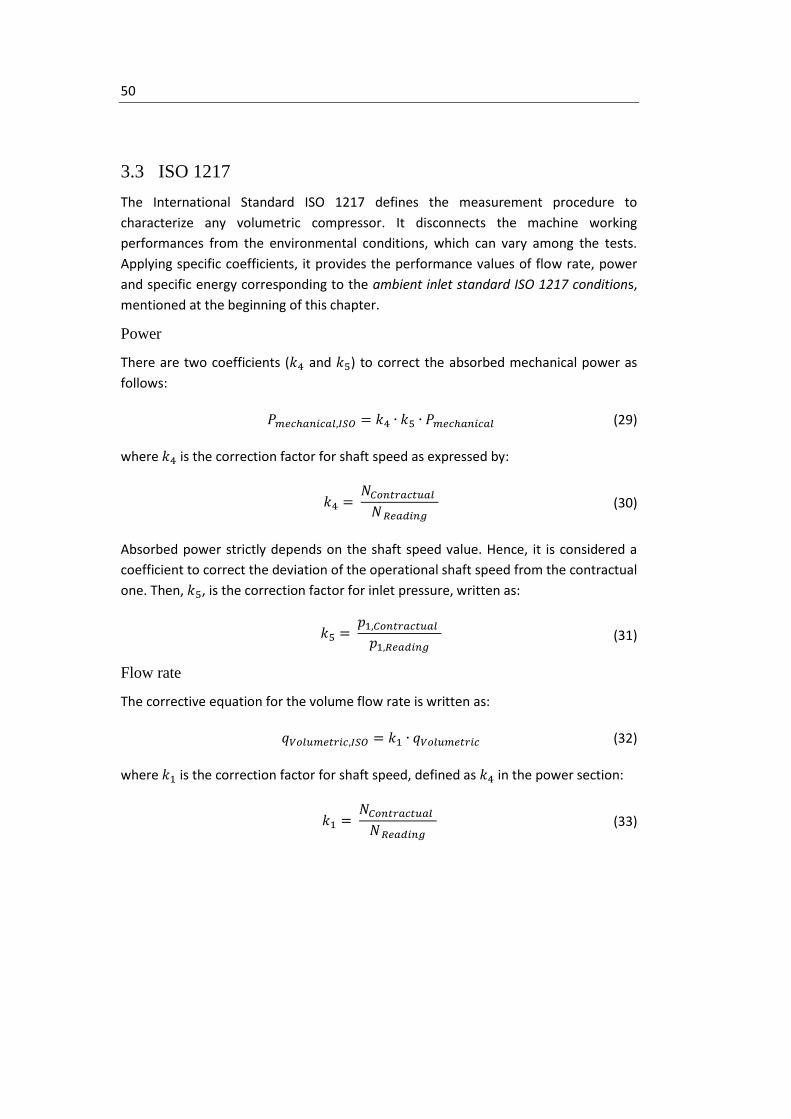
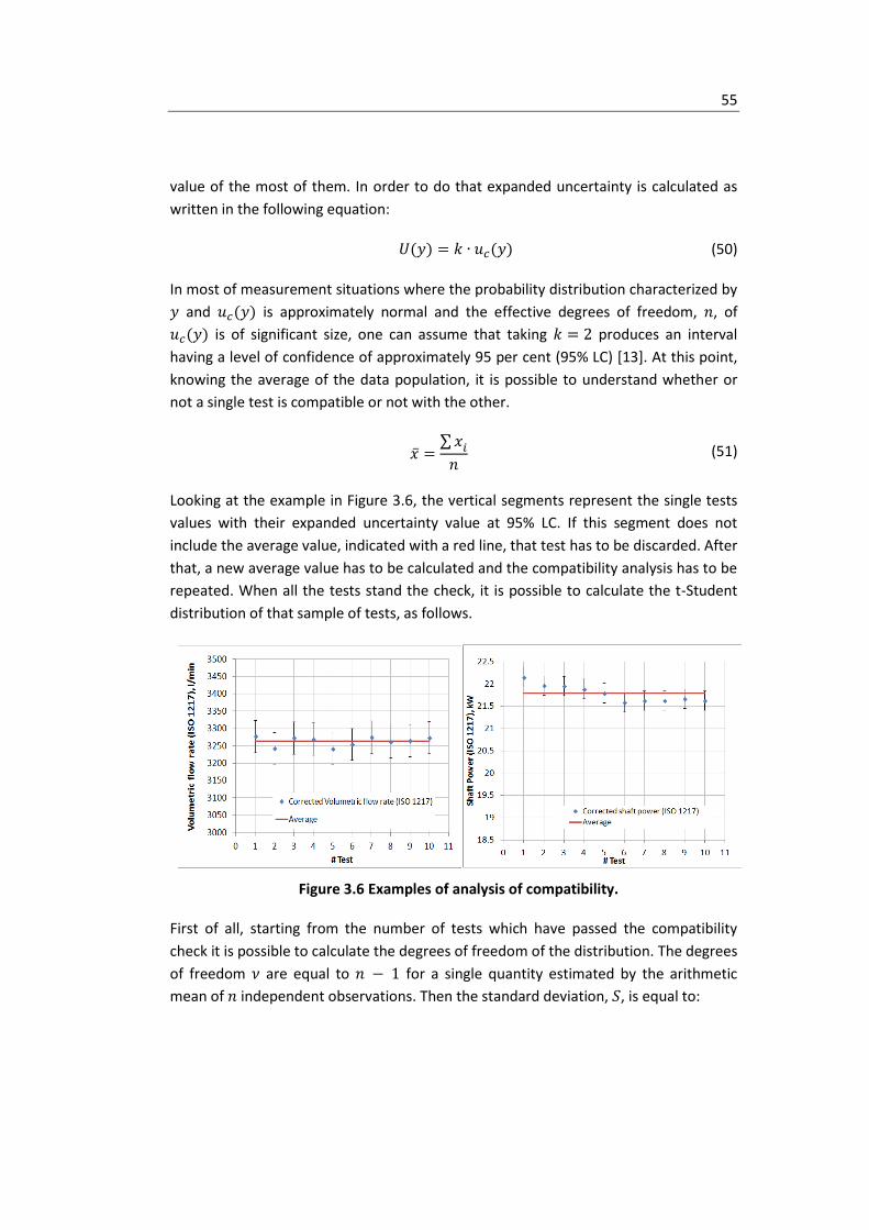
In particular, the compressor core unit can vary in type and size from a small one of
2.5 kW to huge systems with more than 250 MW. As shown in Figure 1.2, there are
two basic compressor types: dynamic and positive-displacement.
Dynamic compressors. They impart velocity energy to continuously flowing air
by means of impellers rotating at very high speeds. The velocity energy is
changed into pressure energy both by the impellers and the discharge
Figure 1.2 A taxonomy of different types of gas compressors.
15
diffusers. In the centrifugal-type compressors, the shape of the impeller
blades determines the relationship between air flow and the pressure
generated, and the compression ratio depends on the shaft angular speed.
Positive-displacement. Within this type of compressors, a given quantity of air
or gas is trapped in a compression chamber and the volume which it occupies
is mechanically reduced, causing a corresponding rise in pressure prior to
discharge. At constant speed, the air flow remains essentially constant with
possible variations in discharge pressure. The reciprocating compressor is an
intermittent flow machine that operates at a fixed volume in its basic
configuration through an alternating movement of a piston inside a cylinder.
Rotary compressor is lighter in weight than the reciprocating compressor and
does not exhibit the shaking forces of the reciprocating type, making the
foundation requirements less rigorous. Even though rotary compressors are
relatively simple in construction, the physical design can vary widely.
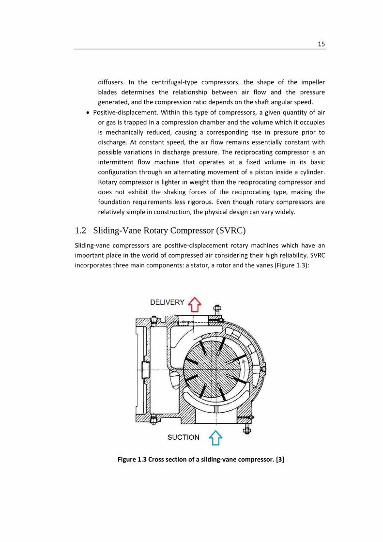
1.2 Sliding-Vane Rotary Compressor (SVRC)
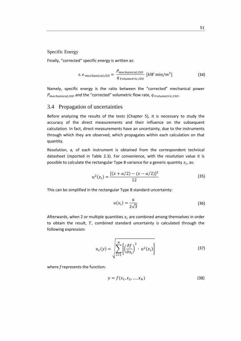
Sliding-vane compressors are positive-displacement rotary machines which have an
important place in the world of compressed air considering their high reliability. SVRC
incorporates three main components: a stator, a rotor and the vanes (Figure 1.3):
Figure 1.3 Cross section of a sliding-vane compressor. [3]
16
The stator, obtained by single fusion, is the shell which contains the compressor
core and the lubrication channels and reservoir.
The rotor, which is the only rotating element, is mounted eccentrically in a
slightly larger hollow cylinder (so that the rotor is tangent to the stator in one
point), and it has a series of radial slots that hold a set of vanes.
The vanes are thin fins as long as the rotor, which are free to move radially
within the rotor slots as the rotor revolves.
Operating principles
The inner compression chamber is closed by a frontal and a rear lid and it contains the
whole process of compression. While operating, vanes maintain contact with the
stator wall by both a centrifugal force, generated as the rotor turns, and by a bottom
up boost provoked by pressurised air. The space between a pair of vanes and the rotor
and the cylinder wall form crescent-shaped cells. As the vanes cross the inlet port, gas
is trapped inside the cells at the minimum pressure. Air is then moved and
compressed circumferentially as the vane pair moves toward the discharge port,
delivering air at the maximum pressure, demanded by utilities.
The rotational shaft speed is an important parameter to be taken into account during
the machine design. In fact, the centrifugal force acting on the vanes is strictly
dependent on the shaft speed of the compressor. Consequently, the quality of the
contact between the vanes and the stator is affected by the variation of this
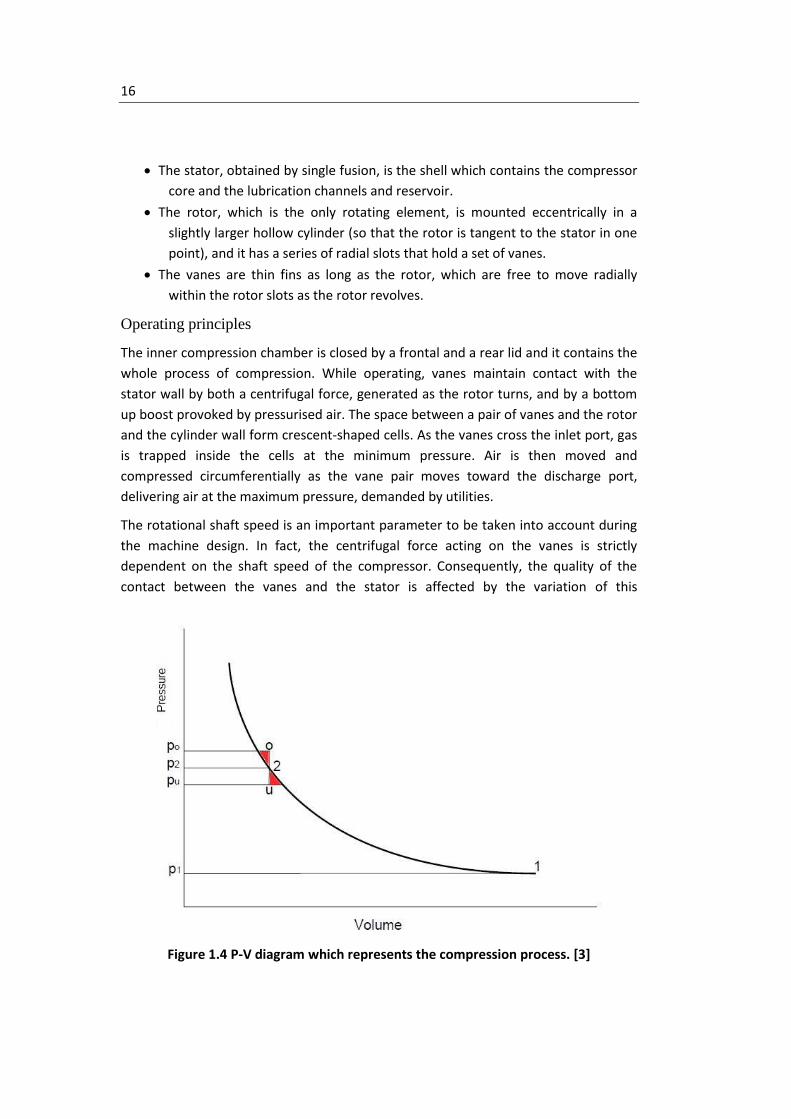
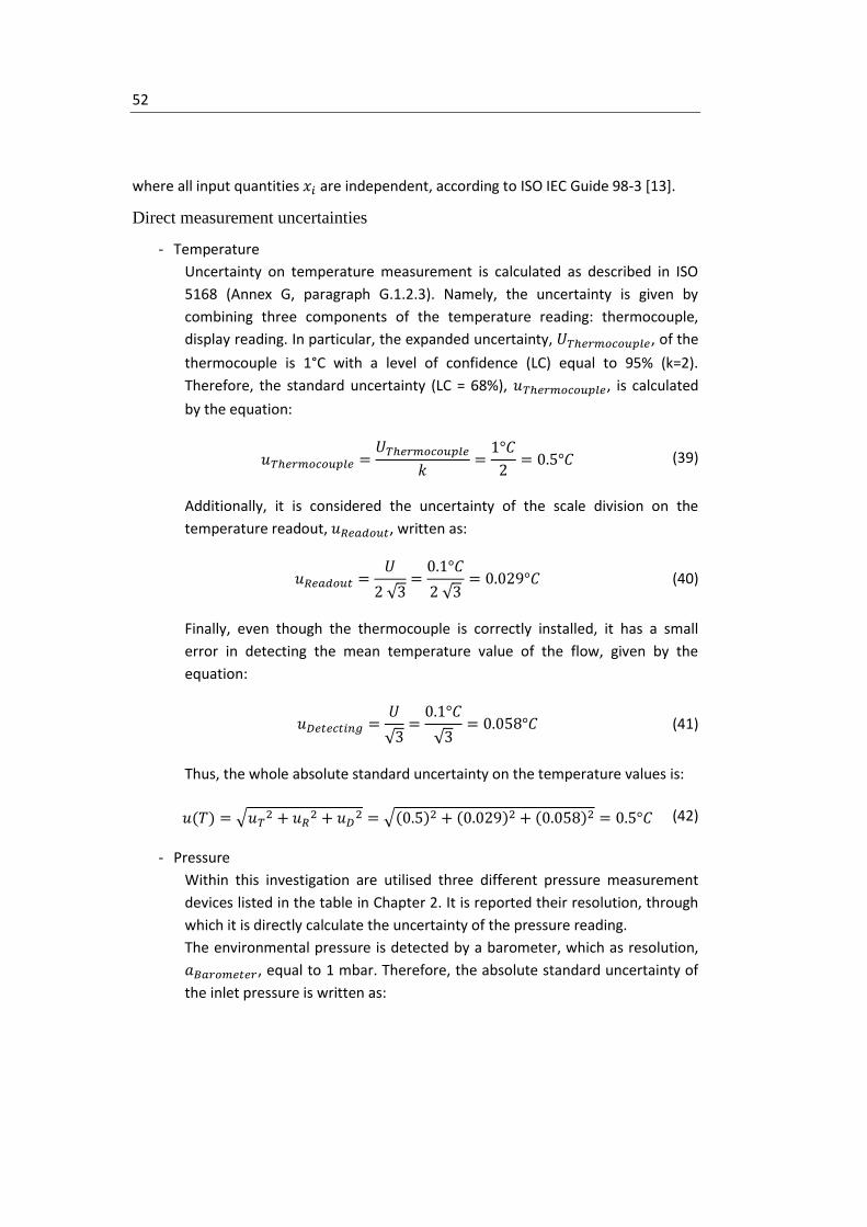
Figure 1.4 P-V diagram which represents the compression process. [3]
17
parameter. A low shaft speed is not able to grant enough air-tight between the top of
the vane and the stator, generating leakages between contiguous cells. At very high
rotational speed, the thin lubricant layer which wraps the vanes risks to be broken.
Therefore, wear rises over materials, causing excessive power losses due to friction.
For efficient compression to take place, the port location must be matched to the
pressure ratio dictated by the application. Figure 1.4 shows an indicator diagram of a
compression cycle. If the port has been optimized for a ratio of , the
compression line is a smooth curve from point 1 to 2. If the external pressure is higher
than the pressure for which the port was designed, so that , then when
the port opens at point 2, discharged air will return to the compressor from the line
and must again be expelled from the compressor. This energy waste is represented by
the red area to the left of the line 0-2. Conversely, if the external pressure ratio is
lower than the pressure ratio for which the port was cut, where , then
the gas will be overcompressed to point 2 and when the port opens, it will expand to
point u. The lost energy is represented by the red area to the right of the line u-2. [3]
Lubrication
As mentioned, this type of compressor must have an external source of lubrication. A
pump is not required for this injection because the pressure of the oil after separation
from the air is sufficient to be re-injected. Oil acts during the compression as:
Lubricant: oil controls the tribology of the compressor: wear, friction and
lubrication of mechanical parts. Actually, the rotor spins into two bushes
which need to be lubricated. As well, the friction among rotor, vanes and
stator affects performances and can provoke some material consumption.
Sealing agent: radial gaps between vanes and the stator, and axial clearances
between vanes and stator need to be filled in order to reduce losses in airflow.
Thermal ballast: during the real compression, heat is transferred to the lubricant
which remains almost totally in the liquid form, which has a great thermal
capacity (thanks to its high density and heat capacity) and large exchange
surface. This liquid significant quantity mitigates the gas temperature rise and,
hence, its compression work.
By absolving these three functions, the oil temperature is induced to increase, as a
consequence of heat exchange from wet air during the compression, worn and friction
of the vanes, sliding and bouncing along rotor and stator surfaces. Lastly, lubricant
executes a protective action on the metallic parts of the compressor, covering them
and, therefore, avoiding corrosion.
18
1.3 Problem definition
As already mentioned, new strategies are undertaken in order to pursue more
efficient power consumptions, rather than the well-known solidity. Therefore, there
could be two possible paths towards improving efficiency:
The first path, more thermodynamical, should operate on the thermal cycle of
compression by means of multiple intercooled stages, in order to maintain a
low air temperature. This presents plant difficulties due to the system’s
complexity. Previous works have produced changes in the size of the oil drops
injected into the compression chamber in order to increase the heat exchange
process
On the other hand, the mechanical path should make it possible to improve the
performances of the machine without varying the cycle of the gas (wet air)
along the compressor. In this dissertation two parallel roads have been taken:
the first one consists in using a different lubricant during the process of air
compression, the second one consists in using a different vane material for the
purpose of the compression.
1.4 Objectives
This investigation aims to study experimentally the impact of two vane materials (cast
iron and aluminium with anodized surface) and of four commercial lubricants
(characterized by different viscosity indexes and additives concentrations) on the
performance of a mid-capacity sliding-vane rotary compressor at five different
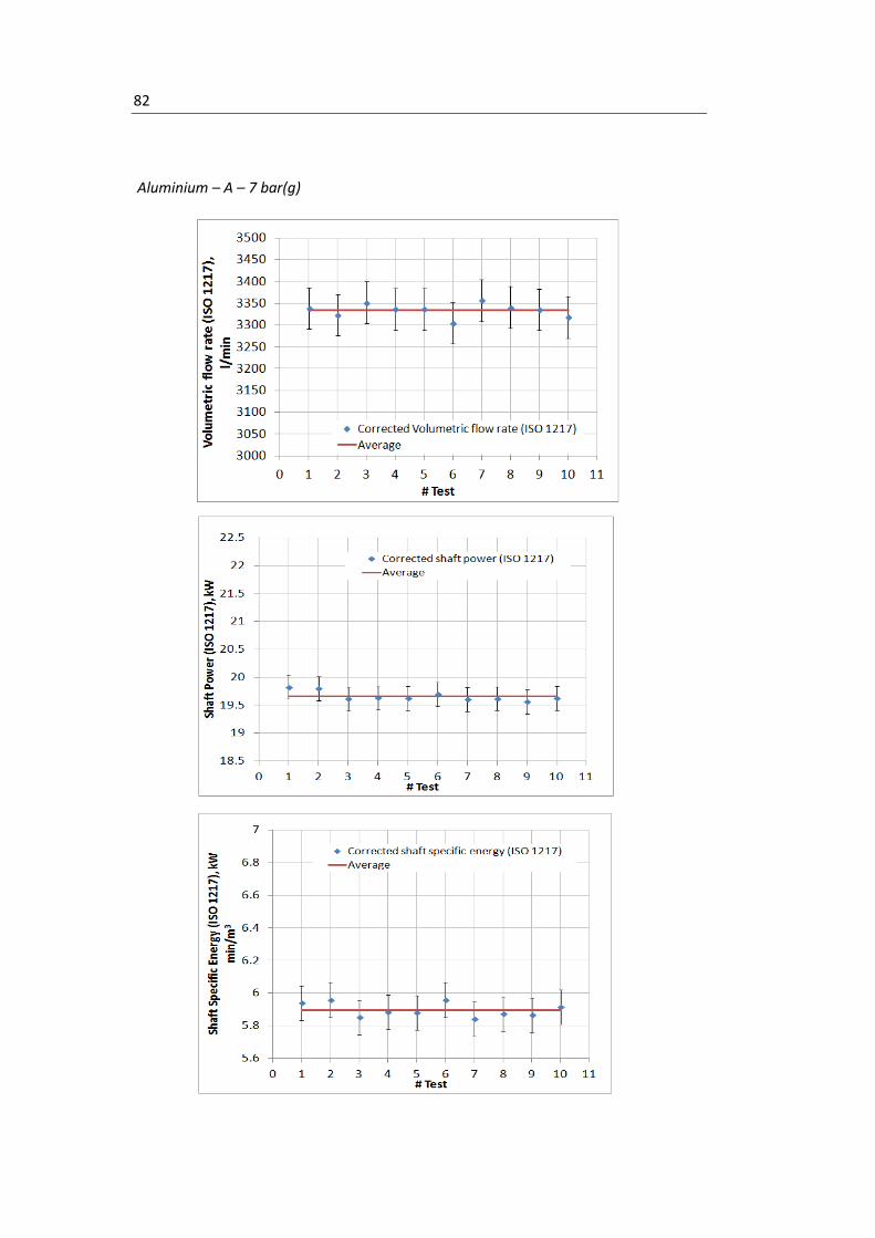
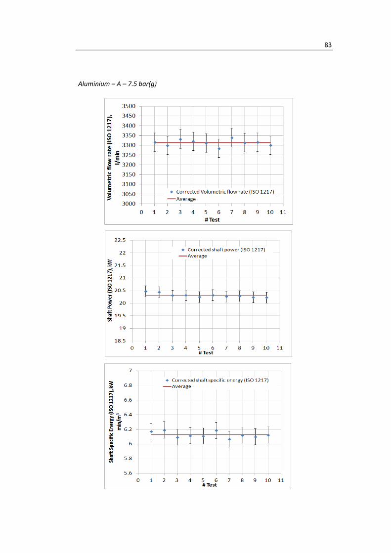
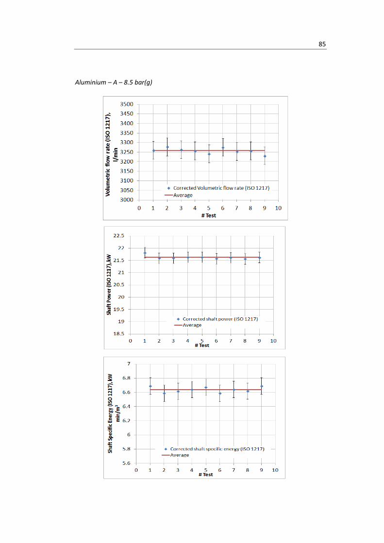
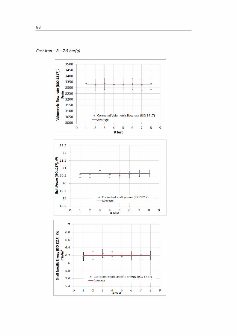
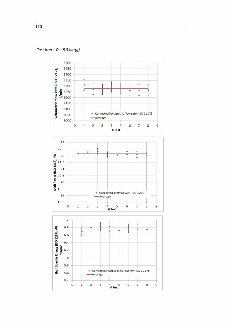
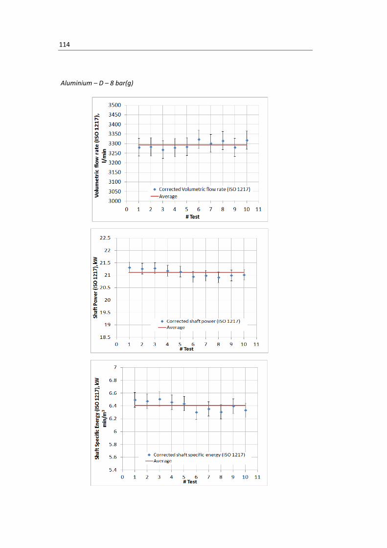
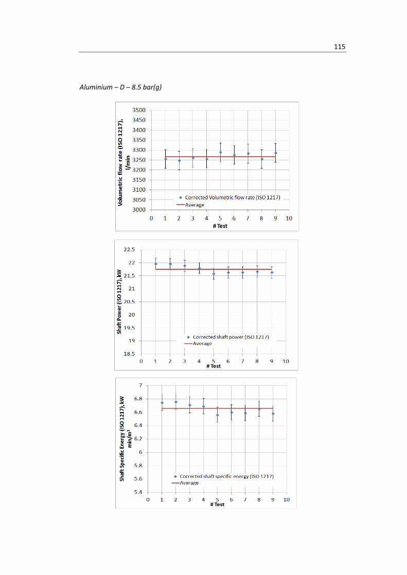
operating pressures. Analysis is carried out of 400 experimental tests on a SVRC.
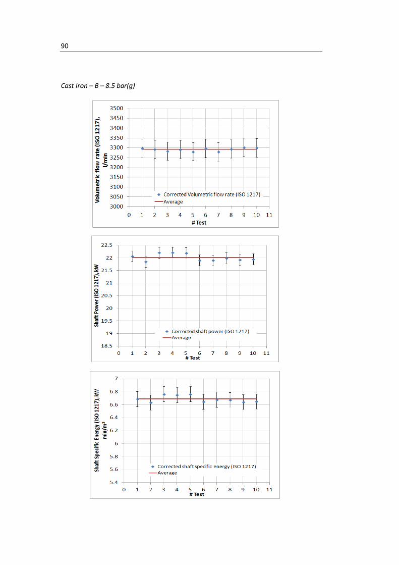
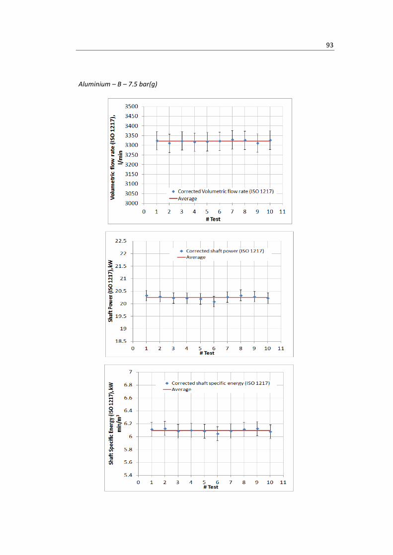
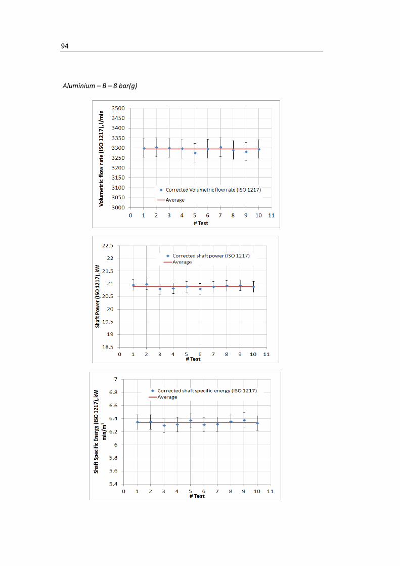
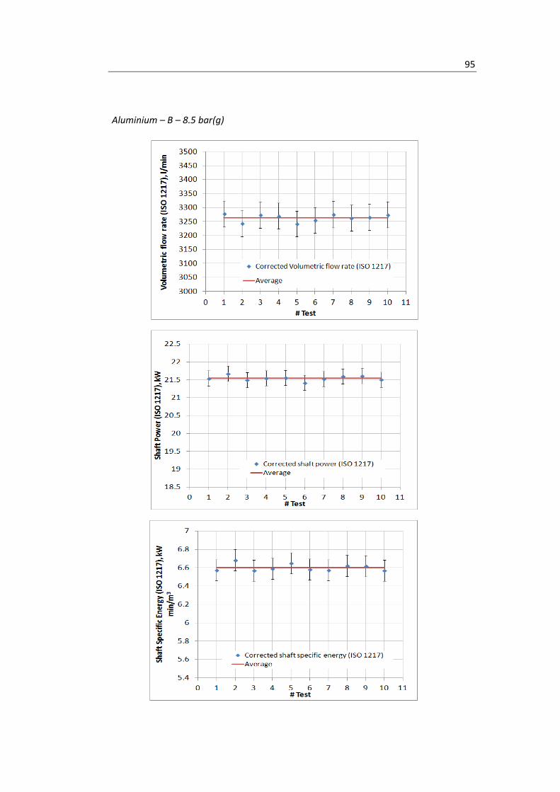
In particular, performance is characterized by the study of the volume flow rate, the
absorbed mechanical power and the mechanical specific energy. Therefore, the main
objectives are the identification of:
possible connections between the SVRC performances and the two different
tested materials;
connections between the SVRC performances and the commercial lubricants
which have been selected for tests;
1.5 Methodology
Tests vary in lubricant, vane material and delivery pressure. They are divided into 40
cases; each of them is replied 10 times in order to grant the repeatability and to
increase the confidence of results. Performance parameters (flow rate, mechanical
19
power, and mechanical specific energy) have been calculated following a standard
procedure which is consistently applied within Mattei®.
Hypothesis is done to proceed with calculation of the air flow through the circuit and
at different conditions. Wet air is considered as an ideal mixture of gases: dry air and
vapour. Dry air is considered as an ideal gas and vapour is considered to follow pure
water behaviours described in IAPWS Formulation.
In order to calculate wet air flow through the compressor, ISO 5167 is applied at the
flow measurement device. This Standard approaches the problem of finding the mass
flow rate through a differential pressure. Afterwards, operational flow rate is
converted into Free Air Delivery (FAD, at the inlet air conditions), before being
standardize at ambient ISO 1217 conditions together with the mechanical power. This
latter conversion permits the comparison between the values of performance, as data
were collected at the same conditions of temperature, pressure and relative humidity.
Uncertainties are calculated for direct measurements according to each instrument
technical datasheet. Propagation of uncertainties is calculated according to ISO 5168
and to ISO IEC Guide 98 (Guide to the Expression of Uncertainty in Measurement,
GUM) for combined quantities and for the compatibility check of results.
To implement the whole calculation procedure, a MATLAB® program is compiled
within this study, starting from the structure of earlier versions, which were developed
within preceding thesis projects [4] [5]. Its functions have a standard input and output
format which simplifies the organization of the code. Moreover, uncertainty
calculations are added within each single function. Lastly, a VBA Excel spreadsheet
workbook is created to collect all the results, to execute the compatibility analysis and
to build graphs of averaged values of performance.
1.6 Structure of the thesis
The following sections are structured as below:
chapter 2 describes in detail the setting up of the experiment. The test bench,
the measuring instruments (their working principle and their uncertainties),
and the data collection procedure are characterized. Furthermore, the
experimental campaign is described: the mid-size compressor utilised to
conduct the tests, the two different materials (cast iron and aluminium with
anodized surface), and four commercial synthetic lubricants (called A, B, C and
D throughout this dissertation).
chapter 3 explains the hypotheses, the Standards and the formulations which
are applied to analyse data and the uncertainty calculation procedure.
20
chapter 4 describes the MATLAB code and the VBA Excel workbook, both
developed during this thesis project.
chapter 5 reports performance results from data analysis and comments on
performance trends. Also some considerations about flow rate measurement
variability with atmospheric conditions are proposed.
chapter 6 presents the conclusions of the project, evaluating whether or not the
objectives have been achieved or not.
chapter 7 proposes suggestions for possible future work and development on
the Mattei® sliding vane compressor.
1.7 Bibliographic Review
Three previous thesis projects are taken into consideration in order to proceed with
this dissertation. In particular, this work resumes the results obtained by Recalcati in
terms of methodology and in terms of vane materials
P. Calvi – Experimental investigation on the effetcs of the oil injection through
an atomised-oil injection system, 2011-2012
In these work, results of a comparison between convectional solid-flow injection and
innovative atomised-oil injection system tested with an experimental rig are shown:
atomization should generate small oil droplets to increase heat exchange and vane
cooling, leading to a decrease of compression work. Nozzles cause the compressor a
saving of energetic consumption and a specific energy increment when they’re
positioned in the closest position to the zone of maximal compression. Keeping oil
nozzles and adding a gear pump to pressurize the oil circuit an increase of air flow is
obtained and in the first part of the compression isothermal process is reached, but
energetic consumption is higher due to the pump. [6]
M. Miggiano – Experimental Campaign for the development and the study of
sliding-vane compressor with modified stator geometry, 2012-2013
In this thesis performance of a modified positive-displacement vane compressor is
evaluated optimizing the stator geometry and a useful calculation tool to process data
is developed. Five versions of the compressor were considered and their performances
compared to estimate the improvement due to the new design of the stator and the
use of a larger intake valve, a wider intake port and a larger exhaust. The volume flow
rates were calculated by using a MATLAB® ad-hoc developed code, taking into
consideration the ISO1217 and ISO5167-3 standards. This code also allows to
determine the specific energy of the compressor and to evaluate the error of the
measurement system. During the tests, the used measuring chain proved some limits
21
concerning the measurement accuracy, therefore, a new highly accurate configuration
of measurement of the flow rate was studied, with the error reduced to 1.55%. [4]
M. Recalcati – Experimental investigation of sliding-vane compressor
performances with diverse vane materials, 2013-2014
This thesis shows how vanes made of different materials (kevlar, glass fiber,
aluminium, drilled iron and iron) affect a displacement compressor performance.
Volumetric flow rate, required shaft power and shaft specific energy were first
calculated and then corrected following ISO 1217 [2] and ISO 5167 [3] guidelines. Data
spreadsheets were later fed to an appropriate programming script written to work
with both Matlab® and GNU/Octave. Results show that the required shaft specific
energy sample average is roughly the same for glass fiber, aluminium and iron, while
kevlar and drilled iron display more significant differences. This work concludes that
simply reducing a vane weight not only is insufficient to improve a compressor
performance, but it can even lead to worse performances. [5]
23
Chapter 2. Experimental Campaign
The laboratory setup, used to carry out the tests within this investigation, includes the
experimental rig with the compressor bench (main unit + electric motor), represented
within the scheme in Figure 2.1. Along this section are firstly presented the air flow
measurement circuit and an oil cool-down circuit. Then, a description of the
instrumentation used to acquire data is proposed and, more in detail, the compressor
equipment. Finally, the data acquisition procedure and the different test
configurations are presented.
2.1 Compressor Equipment
The compressor bench is composed of a compressor with an air-oil candle type
separator, an electric motor mastered by a control panel and finally a radiator
followed by a condensate separator.
Compressor
The device being tested is a Mattei® M111H compressor. Its characteristics are
summarized below:
Packaged compressor. This is a compressor which, according to ISO 1217,
integrates the power source and its transmission, the oil tank and the oil
separation and the air-condensate separator. It is fully piped and wired
internally, including auxiliary items of equipment (in this case only the cooling
radiator) [7].
ERC 22 L outfitting configuration. It is not soundproof and it has a 8 bar(g)
maximum pressure, 7.5 bar(g) operational pressure and requires 22 kWe of
power supply.
This compressor is selected for this project in virtue of its:
mid-sized dimension, which would allow an extension of results to any of
Mattei® compressors (whatever the size);
Table 2.1 M111H dimensions.
Model Length Width Height Weight
[mm] [mm] [mm] [kg] ERC 22 1580 580 970 325
24
good performances in terms of specific energy (around 6.3 kW min /m3);
good solidity and reliability, due to a long experience of test and operation.
The core unit includes the stator and the rotor of the compressor, as described in the
introduction for a standard SVRC (1.2Sliding-Vane Rotary Compressor (SVRC)). The air
suction section is located on the frontal lid, while the delivery section is located on top
of the chamber, linked to the separation unit.
The removal of the frontal lid allows the easy replacement of vanes, while lubricants
are discharged through a lateral valve and refilled from the top of the compression
chamber, in order to set the desired test condition. Furthermore, during every
lubricant replacement, the oil circuit is cleaned thoroughly to prevent contaminations.
Motor
The compressor is coupled with a 22 kWe asynchronous 3 phase motor through a
Figure 2.1 Picture of the experimental compressor outfitting. (Mattei®, 2014)
Table 2.2 Operating features of the sliding-vane rotary compressor M111H.
Rated flow rate, l/min* 3500
Rated working pressure, bar(g) 7.5 Rated power, kWe 22
Nominal rotor speed, rpm 1500 *Standard conditions as per ISO 1217 Standard acceptance
25
flexible joint which grants good alignment and low power absorption.
The whole machine supplies constant air flow at the nominal rotor speed of 1500 rpm.
Such speed is set by the 50 Hz (4 electric poles) frequency of the electric power grid.
Oil Separation
The outside of the compressor shows two stacked cylinders (Figure 2.1Figure 2.):
The lower one contains the pumping unit and acts as primary mechanical oil
separation and, at the same time, as oil tank (Figure 2.2). The air intake enters
the frontal lid, whereas the channel of cold oil flows in through the lateral
surface of the stator. When the air-oil mixture exits the chamber, the flow
meets a labyrinth path which makes it decelerate and change direction. In this
way, oil deposits and it can be easily directed toward the radiator, whereas
the air flow heads toward the upper cylinder.
The upper cylinder, placed above the main body of the machine, consists of 3
coalescent filters for the secondary oil separation. They absorb the residual oil
vapours from the air flow. Finally, the air duct leaves the upper cylinder after
the filtration step, heading towards the radiator.
Figure 2.2 CAD Drawing of the pumping unit. (Mattei®, 2014)
26
Hence, oil separation is distributed over multiple steps: the first one, which is
mechanical, is the more substantial, while the second one is reduced.
Radiator
As just mentioned, the experimental version of the machine is equipped with an
aluminium air-radiator. This unit is divided into two sections under the same fan
airflow: one for the oil cooling and the other one for the air cooling. The fan is
powered by the same electric motor as the compressor, which is connected to the
power grid. It also slightly serves as a motor cooler, as its generated air-stream is
directed toward the motor shell.
Moreover, the radiator is equipped with a condensate separator (the first along the air
circuit) to discharge water. At this point of the circuit, water forms due to the heavy
compression stage. At the same time, temperature increment during compression is
not enough to permit the water vapour to keep its gas phase: it condensates, thus
becoming liquid water. This process is what makes the hypothesis of saturated air
possible (100% of Relative Humidity).
2.2 Air - Oil Circuit
BWet air enters from the frontal lid into the compression chamber, it is compressed
and it flows out mixed with lubricant towards the mechanical separation. After this
step, air goes through the coalescent oil filters and, almost without oil, it flows
towards the radiator. At this point, there is a first condensate separator, a compressed
air tank and a second condensate separator before the flow measurement pipe.
As mentioned in section 1.2, oil acts during the compression as lubricant, sealing agent
and thermal ballast. These three functions induce the temperature of the oil to
increase, as a consequence of heat exchange, worn and friction of the vanes, which
slide and bounce along the stator surface.
Oil starts its path within the machine from the injection into the compressor chamber
through an injection case, which has 5 holes axially arranged (standard Mattei®
injectors), which make the oil enters the compression chamber radially, mixing with
air. Air and oil mixture at very different temperature condition causes a loss within the
efficiency of the compression. Thus, holes are located in the last compartments (250°
from the suction section in the rotation direction), where air is already at high
pressure and high temperature.
Leaving the compression chamber, the high temperature air-oil flow gets into a cavity
around the pumping unit, filled with maze tunnels. Here, a mechanical separation
27
takes place and for gravity action, oil sinks to the bottom whereas air occupies the top.
Oil is drained out of the interspaces and send into the radiator, where it is cooled
down by the fan.
However, some oil gets trapped in the air flow and it requires a further separation.
This happens in the upper cylinder of the machine, through three coalescing oil filters
which release air almost without oil (1-3 ppm, with 1ppm= 1.2 mg/m3 at Free Air
Delivery conditions, F.A.D.). The oil held by these filters is redirected directly to the
chamber, with no refrigeration.
2.3 Laboratory Instrumentation
In order to verify experimentally the performances of materials and lubricants, a test
rig based on a commercial 22-kW SVRC was assembled. The experimental rig, shown
in, employs the necessary instrumentation to measure air temperatures and pressures
along the compression, the delivered volume flow rate, lubricant temperatures and
pressures along the process, and, finally, shaft torque and rotational speed. The
experimental setup is design to evaluate the compressor performances while varying
the delivery pressure.
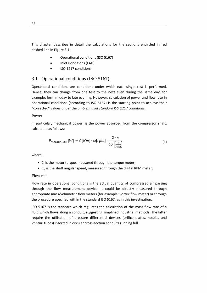
In particular, the mechanical power is calculated as product of shaft torque and
rotational speed measured using a flange torque meter installed between the
compressor and the electric motor. A Kistler 4504B1KB1N1 torque meter (Full Scale of
1000 Nm, Accuracy ±0.5% FS) is controlled by the evaluation instrument Kistler CoMo
Torque Type 4700A.
The electronic data acquisition is performed thought the National Instruments cDAQ-
9178 wired to a personal computer. LabView Signal Express 2011® is used to carry out
the measurements.
Table 2.3 Instrumentation List
Instrumentation Measured quantity Accuracy Model Manufacturer
Barometer p_barometric ±1 mbar 102 Fischer Manometer p_chamber ±0.05 bar - Spriano Hygrometer UR ±1% Supratherm Barigo Thermocouple T_in ±0.1°C T Model Tersid Thermocouple T_chamber ±0.1°C T Model Tersid Thermocouple T_device ±0.1°C T Model Tersid Water column p_static ±1mmH2O - - Water column p_differential ±1mmH2O - - Torque meter Torque ±0.1 Nm 4504B1KB1N1 Kistler Digital RPM Meter Shaft speed ±1 rpm - IDF
28
Shaft speed value has been determined through a Digital rpm meter with an accuracy
of 1 rpm.
A Fischer barometer and a Spriano analogical Manometer have been used to evaluate
respectively room pressure and chamber pressure.
Temperature values have been estimated with three thermocouples located
respectively:
at the suction port (input temperature);
at the oil separation (chamber temperature);
at the pressure differential device (device pressure).
Finally, to gauge relative humidity a Barigo Hygrometer has been used.
2.4 Test Acquisition
The collection of data follows a very standard procedure described below. It consists
of general steps, typical for every compressor analysis, and specific steps for this test
bench.
Figure 2.3 Instrumentation rig. (Mattei®, 2014)
29
Instrumentation check
1) Before turning the apparatus on, it is highly recommended to check that all the
instrumentation is accessible and ready to operate as required.
2) All the electric devices have to be plugged in: computer, temperature display,
torque/rpm viewer. They in turn have to be connected to the corresponding sensors:
thermocouples and torque meter.
3) The presence of water into the columns of the pressure gauge has to be double
checked. The of connection of this latter to the pressure differential device has to be
checked as well: the upstream intake to the static column, and the downstream intake
to the differential one. Both of them have to be closed with the respective valve in
order to avoid the spillage of water when powering the system.
Ignition
4) First of all, the recirculation valve at the suction section has to be open, to allow
the open circuit operation at the start.
5) Then it is possible to plug in the measurement system (220V switch), taking
care to set to zero the electric devices.
6) At this point also the 380V switch can be turned on, wait for the digital control
panel to be ready, and finally push the power on button.
7) Let the compressor run for 10-20 seconds and then the recirculation valve has
to be turned off. It is good practice to set the throttling valve at the maximum
opening, in order to reduce the risk to reach a very high pressure as long as the
machine is cold.
8) Next step is to regulate the throttling valve to obtain the required backpressure,
e.g. 7.5 bar-g.
9) Now it is possible to open the water column pressure gauge valves.
10) When the speed condition is stable (after about 1h) at the previously set
backpressure, the chamber temperature should be constant (or very slowly fluctuating
around a value). It is now possible to acquire test data, reporting them onto a proper
“Test Reports” paper, or directly in the input Excel file for the MATLAB code “RnD”.
Shutdown
11) Before turn off the power, it is good practice to open again the throttling valve
down to the minimum chamber pressure. Then, also the recirculation valve has to be
opened.
30
12) When the chamber pressure reaches the 1.5 bar-g is it possible to turn the
power off from the digital control panel.
Rig rearrangement
13) All the valves between the differential pressure device and the water columns
have to be closed.
14) It is possible to turn off the 380V switch.
15) After the computer shut down, also the 220V switch can be turned off.
2.5 Experimental Campaign
This investigation is based on an extensive experimental campaign. Research is carried
out involving 400 tests, performed on the Mattei® M111H Compressor. Tests are
performed combining:
2 types of vane materials: cast iron and aluminium;
4 types of lubricants: A, B, C, D;
5 values of pressure: 6.5, 7, 7.5, 8, 8.5.
Each combination of material, lubricant and pressure is repeated 10 times in order to
obtain the repeatability for all the 40 possible conditions. For each condition, tests are
carried out on at least two different days (from 9:00 to 18:00), so that one may trace
the average behaviour of the machine, independently from ambient pressure,
temperature or humidity conditions at different times of the day.
In order to delete the effect of any correlation between tests, their sequence is
randomized. The only fixed parameters are:
Chamber operating temperature of about 85°C
Nominal Rotor speed of about 1500 rpm
Modifications of parameters are introduced by operating on the compressor bench
(interchanging vane materials and lubricants) and on the pressure regulating valve
(placed immediatly after the air pressurized tank).
31
2.6 Vane materials
Besides the rotor, vanes are the only part of the compressor subject to motion during
the whole compression process. For this reason, in addition to their reduced thickness
(of about 5 mm, Figure 2.4), they are the most critical components of a SVRC and they
are among the main objects of study in this field.
Due to the force system (in Figure 2.5) that generates during the operation of the
compressor, vanes are exposed to:
Friction, of the vane which slides along the slot (two contact edges along the
rotor section) and hits the stator shell with its radius of curvature (R = 9.5
mm).
Wear, as a result of friction, causes the adaptation of the vanes to their slots
and to the stator contact during operation. In particular, the most significant
abrasion can be noticed on the back of the vane (due to the back of the vane
sliding on the rotor upper edge) and on the top of it (where the vane hits the
stator). Wear leads to an auto-adjustment of the contact resistance. This
phenomenon ensures less contact between surfaces (vanes-rotor, vanes-
stator) and after some time of running test, performances start improving: in
particular, the power consumption decreases by about 2%.
Figure 2.4 Drawing of the pumping unit. (Mattei®, 2014)
32
In this specific compressor (M111H), there are 7 double vanes, making a total of 14
“half-vanes”. As a consequence of its mid-size, double vane configuration is necessary
to avoid rotation or flexion of the vanes within each slot. On the other hand, the
double vane configuration presents one more leakage source in between the two half-
vanes, which can produce a loss in flow rate (for some more elastic material it is
possible to apply a single vane through the entire rotor).
In order to try to improve the impact of the vanes on the performance parameters of
the compressor (flow rate and power consumption), a different vane material is
tested, rather than the standard one, so that the two options are:
cast iron vanes (CIV), standard
aluminium alloy vanes (AlV), non-standard
Figure 2.5 Contact edges of the vane. (Mattei®, 2015)
33
The main features of the chosen materials are listed in (Table 2.4).
Cast iron
Cast iron is primarily composed of iron (Fe), carbon (C) and silicon (Si). Its structure is
crystalline and relatively brittle but overall it offers better mechanical properties than
aluminium. In fact, it is readily machined and, additionally, the machined surfaces are
resistant to sliding wear thanks to their hardness.
This is the most adopted material for this type of compressor because of its surface
hardness, which allows a good worn resistance. Furthermore, it has low coefficients of
expansion, so that gaps are minimized and during transient phases (especially
powering the compressor) leakages are reduced. For these reasons this material is
usually used to produce the vanes for SVRC.
Furthermore, cast iron has:
high thermal conductivity, it allows good heat transmission between contiguous
air volumes (more uniform temperature along the vane section);
low modulus of elasticity, it makes vanes brittle and fragile and therefore less
subject to deformation under stress;
ability to withstand thermal shock, this property is useful for fast ignition stages,
during which temperature increases greatly in a short time.
Aluminium
On the other hand, aluminium is remarkable because of its low density. As the weight
of the vane directly affects the friction losses of the SVRC, this dissertation investigates
experimentally the effect of the reduction of the vane weight on the compressor
efficiency.
Table 2.4 Properties of chosen vane materials. (S. Murgia et al., 2015)


![[Quarteroni, Saleri] - Introduzione Al Calcolo Scientifico](https://static.documents.pub/doc/80x56/55cf9ba8550346d033a6e6cc/quarteroni-saleri-introduzione-al-calcolo-scientifico.jpg)

