Politecnico di Milano School of Industrial and … di Milano School of Industrial and Information...

Politecnico di Milano

School of Industrial and Information Engineering

Master of Science in Aeronautical Engineering

Leonardo Cozzubo Gonçalves

Ramjet vehicle and trajectory modeling for transatmospheric propulsion missions

Master of Sciences Thesis

Supervisor: Prof. Dr. Filippo Maggi

Co-supervisor: Prof. Dr. Marcos Pimenta

Milan, Italy

April 2017

Leonardo Cozzubo Gonçalves

Ramjet vehicle and trajectory modeling for transatmospheric propulsion missions

Master Thesis presented at Politecnico di Milanoas part of requirements of Master of ScienceProgram

Supervisor: Prof. Dr. Filippo MaggiCo-supervisor: Prof. Dr. Marcos Pimenta

Milan, ItalyApril 2017

Acknowledgements

Special thanks to my parents, who have always inspired and encouraged me regardlessall the difficulties.

To my grandmother, who has always been by my side.

To my godparents, official or not, who have always helped me.

To my friends, from Brazil, Italy or any other country.

To Professors Filippo Maggi and Marcos Pimenta, for the support and guidance.

Abstract

There is a growing interest on commercial exploration of LEO (Low Earth Orbit). New solu-tions for launching small satellites are arising. One of them uses a vehicle launched from asupersonic aircraft. After decoupling there are two flight phases: the first is based on Ramjettechnology and the second is based on conventional rocket system.The main advantage of thissolution respect to the traditional ones is a higher specific impulse during atmospheric flight,as air is used as oxidizer and doesn’t need to be carried from launching, which translates intoa vehicle mass saving. It’s necessary to have a second phase of conventional rocket system inorder to obtain thrust at high altitudes where the air is too rarefied to allow airbreathing enginesoperation.

This work is concentrated on the Ramjet stage and has the objective of producing a tool thatcan be used in the preliminary phase of real projects by evaluating different configurations andmission designs. It begins with a theoretical study of internal ballistics and of the trajectory withconstant flight path. The Modelica® routine is implemented to simulate this phase and there isthe determination of the parameters to accomplish the mission. Simulation results are discussedand a sensitivity analysis is performed for the internal configuration as well as for trajectoryparameters.

Keywords: simulation, Ramjet, trajectory, propulsion.

List of Figures

Figure 1 – Basic schematic configurarion of a Ramjet . . . . . . . . . . . . . . . . . . 16Figure 2 – Scheme of the studied DR - 1. Air intake; 2. Gas generator; 3. Combustion

chamber; 4. Supersonic nozzle . . . . . . . . . . . . . . . . . . . . . . . . 17Figure 3 – Normal and oblique shocks scheme at Ramjet inlet . . . . . . . . . . . . . . 18Figure 4 – Intake operation regimes . . . . . . . . . . . . . . . . . . . . . . . . . . . 18Figure 5 – Scheme of a variable geometry inlet . . . . . . . . . . . . . . . . . . . . . 19Figure 6 – Plot of air intake model . . . . . . . . . . . . . . . . . . . . . . . . . . . . 20Figure 7 – Different types of air inlets for Ramjet vehicles. They are:(a) Nose (b) Chin,

(c) Frontal cruciform axissimetric, (d) Rear cruciform axissimetric, (e) Axis-simetric under the wing, (f) Double bidimensional, (g) Axissimetric underthe body and (h) Bidimensional under the body. . . . . . . . . . . . . . . . 20

Figure 8 – Evolution of transversal section of solid fuel grain with central perforation . 23Figure 9 – Evolution of transversal geometry of the grain and its thrust throughout

combustion . . . . . . . . . . . . . . . . . . . . . . . . . . . . . . . . . . 24Figure 10 – Convergent-divergent diffuser operating regimes . . . . . . . . . . . . . . . 26Figure 11 – Pressure profile in mbar respect to the variation of geometric altitude, from 0

to 700 km. . . . . . . . . . . . . . . . . . . . . . . . . . . . . . . . . . . . 28Figure 12 – Temperature profile in K respect to the variation of geopotential altitude,

from 0 to 90km. . . . . . . . . . . . . . . . . . . . . . . . . . . . . . . . . 28Figure 13 – Reference frames - Earth-fixed or inertial and Missile body-fixed . . . . . . 30Figure 14 – Scheme of drag decomposition . . . . . . . . . . . . . . . . . . . . . . . . 35Figure 15 – Drag coefficient variation of a V-2 rocket respect to Mach number and angle

of attack variation . . . . . . . . . . . . . . . . . . . . . . . . . . . . . . . 36Figure 16 – Lift coefficient variation of a V-2 rocket respect to Mach number and angle

of attack variation . . . . . . . . . . . . . . . . . . . . . . . . . . . . . . . 37Figure 17 – Relationship between center of gravity and center of pressure on vehicle

stability. In (a) there is a case with a center of pressure below the center ofgravity (a stable case), in (b) center of pressure above center of gravity (aninstable case) . . . . . . . . . . . . . . . . . . . . . . . . . . . . . . . . . 38

Figure 18 – Representation of the six degrees of freedom of the vehicle . . . . . . . . . 39Figure 19 – Forces scheme for an ascending trajectory in a stationary planet . . . . . . . 42Figure 20 – Scheme for the relationship between submodels . . . . . . . . . . . . . . . 45Figure 21 – Drag coefficient curves used in the interpolation . . . . . . . . . . . . . . . 48Figure 22 – Lift coefficient curves used in the interpolation . . . . . . . . . . . . . . . . 48Figure 23 – Evolution of altitude in time for Scenario 1 . . . . . . . . . . . . . . . . . . 52Figure 24 – Distance respect to ground for Scenario 1 . . . . . . . . . . . . . . . . . . . 53

Figure 25 – Evolution of Mach number for Scenario 1 . . . . . . . . . . . . . . . . . . 53Figure 26 – Evolution of velocity for Scenario 1 . . . . . . . . . . . . . . . . . . . . . . 54Figure 27 – Evolution of forces acting in the vehicle for Scenario 1 . . . . . . . . . . . 54Figure 28 – Mass variation for Scenario 1 . . . . . . . . . . . . . . . . . . . . . . . . . 55Figure 29 – Atmospheric air density variation for Scenario 1 . . . . . . . . . . . . . . . 56Figure 30 – Evolution of thrust for Scenario 1 . . . . . . . . . . . . . . . . . . . . . . . 56Figure 31 – Evolution of ambient pressure for Scenario 1 . . . . . . . . . . . . . . . . . 57Figure 32 – Evolution of internal pressure for Scenario 1 . . . . . . . . . . . . . . . . . 57Figure 33 – Thrust decomposition for Scenario 1 . . . . . . . . . . . . . . . . . . . . . 58Figure 34 – Comparison of jet exit section and ambient pressures for Scenario 1 . . . . . 58Figure 35 – Variation of air, fuel and total mass flows for Scenario 1 . . . . . . . . . . . 59Figure 36 – Specific impulse variation for Scenario 1 . . . . . . . . . . . . . . . . . . . 59Figure 37 – Fuel mass variation for Scenario 1 . . . . . . . . . . . . . . . . . . . . . . 60Figure 38 – Air to fuel ratio variation for Scenario 1 . . . . . . . . . . . . . . . . . . . 60Figure 39 – Evolution of combustion chamber temperature for Scenario 1 . . . . . . . . 61Figure 40 – Jet and flight Mach numbers comparison for Scenario 1 . . . . . . . . . . . 61Figure 41 – Jet and external air temperature comparison for Scenario 1 . . . . . . . . . 62Figure 42 – Jet and flight velocities comparison for Scenario 1 . . . . . . . . . . . . . . 62Figure 43 – Thrust comparison on initial mass analysis . . . . . . . . . . . . . . . . . . 64Figure 44 – Internal pressure comparison on initial mass analysis . . . . . . . . . . . . 64Figure 45 – Thrust comparison on throat area sensitivity analysis . . . . . . . . . . . . . 65Figure 46 – Mass flow comparison on throat area sensitivity analysis . . . . . . . . . . . 65Figure 47 – Thrust comparison on initial altitude sensitivity analysis . . . . . . . . . . . 66Figure 48 – Pressure profile respect to altitude . . . . . . . . . . . . . . . . . . . . . . . 67Figure 49 – Thrust comparison on initial velocity sensitivity analysis . . . . . . . . . . . 68Figure 50 – Internal pressure comparison on initial velocity sensitivity analysis . . . . . 68Figure 51 – Thrust comparison on flight path angle sensitivity analysis . . . . . . . . . . 69Figure 52 – Velocity comparison on flight path angle sensitivity analysis . . . . . . . . . 70Figure 53 – Thrust comparison on front area sensitivity analysis . . . . . . . . . . . . . 71Figure 54 – Thrust comparison on burning area sensitivity analysis . . . . . . . . . . . . 72Figure 55 – Thrust comparison on Vieille’s law constant sensitivity analysis . . . . . . . 73Figure 56 – Air to fuel ratio comparison on Vieille‘s law constant sensitivity analysis . . 73Figure 57 – Combustion chamber temperature comparison on Vieille’s law constant sen-

sitivity analysis . . . . . . . . . . . . . . . . . . . . . . . . . . . . . . . . 74Figure 58 – Thrust comparison of Vieille‘s law exponent sensitivity analysis . . . . . . . 75Figure 59 – Ait to fuel ratio comparison on Vieille’s law exponent sensitivity analysis . . 75

List of Tables

Table 1 – Gas generator parameters . . . . . . . . . . . . . . . . . . . . . . . . . . . . 46Table 2 – Simulation Parameters . . . . . . . . . . . . . . . . . . . . . . . . . . . . . 51Table 3 – Sensitivity analysis of the initial mass . . . . . . . . . . . . . . . . . . . . . 63Table 4 – Sensitivity analysis of throat area . . . . . . . . . . . . . . . . . . . . . . . 64Table 5 – Sensitivity analysis of the initial altitude . . . . . . . . . . . . . . . . . . . . 66Table 6 – Sensitivity analysis of the initial velocity . . . . . . . . . . . . . . . . . . . 67Table 7 – Sensitivity analysis of flight path angle . . . . . . . . . . . . . . . . . . . . 69Table 8 – Sensitivity analysis of vehicle frontarea . . . . . . . . . . . . . . . . . . . . 70Table 9 – Sensitivity analysis of burning area . . . . . . . . . . . . . . . . . . . . . . 71Table 10 – Sensitivity analysis of fuel release law constant . . . . . . . . . . . . . . . . 72Table 11 – Sensitivity analysis of the fuel releaselaw exponent . . . . . . . . . . . . . . 74

List of abbreviations and acronyms

AP Ammonium Perchlorate

CFD Computational Fluid Dynamics

DAE Differential Algebraic Equation

DR Ducted Rocket

GPS Global Positioning System

HTPB Hydroxyl-terminated Polybutadiene

LEO Low Earth Orbit

NASA National Aeronautics and Space Administration

NED North-East-Down reference system

ODE Ordinary Differential Equation

SPLab Space Propulsion Laboratory and Nanoenergetics - Politecnico di Milano

List of symbols

ab Vieille-Saint Robert law constant

Ab Burning area

ac Body acceleration

Ae Diffuser exit area

α Angle of attack

αt Angle between x-axis and thrust direction

a Speed of sound

A∗ Throat area

Cda Axial drag coefficient

Cd Drag coefficient

Cl Lift coefficient

Cn Normal force coefficient

Cp Specific heat at constant pressure

Cv Specific heat at constant volume

d0 Port diameter

Da Axial drag force

m f Fuel mass flow rate

D Drag

F Force

γ Specific heat ratio

gn Gravity acceleration at Earth surface

g Ratio of mass through port to mass efflux from surface

g Local gravity acceleration

G Mass flux through port

he Enthalpy

h Altitude

ht Total enthalpy

I Moment of inertia

Isp Specific impulse

Lc Characteristic length

L Lift force

Ma0 Flight Mach number

Mae Mach number at exit section

Ma Mach number

H Heaviside function

M Molar mass

µ Gas dynamic viscosity

Mx Angular momentum respect to x-axis

My Angular momentum respect to y-axis

Mz Angular momentum respect to z-axis

n Vieille-Saint Robert law exponent

N Normal aerodynamic force

ν Kinematic viscosity

p0 Stagnation pressure

pc Pressure at gas generator

pe Pressure at nozzle exit

φ Roll angle

πd Total pressure ratio at the intake

Plong Weight force at longitudinal direction

ψ Yaw angle

p Absolute pressure

P Roll angular velocity

pt Total pressure

q Quaternion

Q Pitch angular velocity

rb Burning rate of pyrolant grain surface

Re Reynolds dimensionless number

ρp Solid density

ρ Fluid density

r Distance between vehicle and center of Earth

R Gas constant

R Yaw angular velocity

Rt Earth radius

S Reference area for aerodynamic forces calculation

θ Pitch angle

T Absolute temperature

Tt Total temperature

u Velocity on x-axis

v f Fluid velocity

v Velocity on y-axis

w Velocity on z-axis

Contents

1 Introduction . . . . . . . . . . . . . . . . . . . . . . . . . . . . . . . . . . 131.1 Motivation . . . . . . . . . . . . . . . . . . . . . . . . . . . . . . . . . . . 131.2 Objectives . . . . . . . . . . . . . . . . . . . . . . . . . . . . . . . . . . . 151.3 Work outlines . . . . . . . . . . . . . . . . . . . . . . . . . . . . . . . . . 15

2 Literature Review . . . . . . . . . . . . . . . . . . . . . . . . . . . . . . 162.1 Ramjet vehicle . . . . . . . . . . . . . . . . . . . . . . . . . . . . . . . . 162.1.1 Air Inlet . . . . . . . . . . . . . . . . . . . . . . . . . . . . . . . . . . . . 172.1.2 Gas Generator . . . . . . . . . . . . . . . . . . . . . . . . . . . . . . . . 202.1.3 Combustion Chamber . . . . . . . . . . . . . . . . . . . . . . . . . . . . 252.1.4 Supersonic nozzle . . . . . . . . . . . . . . . . . . . . . . . . . . . . . . . 252.2 Atmosphere . . . . . . . . . . . . . . . . . . . . . . . . . . . . . . . . . . 272.3 Trajectory . . . . . . . . . . . . . . . . . . . . . . . . . . . . . . . . . . . 292.3.1 Spatial Reference . . . . . . . . . . . . . . . . . . . . . . . . . . . . . . . 292.3.1.1 Euler angles . . . . . . . . . . . . . . . . . . . . . . . . . . . . . . . . . . 302.3.1.2 Cosine Matrix . . . . . . . . . . . . . . . . . . . . . . . . . . . . . . . . . 312.3.1.3 Quaternions . . . . . . . . . . . . . . . . . . . . . . . . . . . . . . . . . . 322.3.2 Forces acting on the vehicle . . . . . . . . . . . . . . . . . . . . . . . . . 332.3.2.1 Weight . . . . . . . . . . . . . . . . . . . . . . . . . . . . . . . . . . . . . 332.3.2.2 Thrust . . . . . . . . . . . . . . . . . . . . . . . . . . . . . . . . . . . . . 342.3.2.3 Aerodynamic Forces . . . . . . . . . . . . . . . . . . . . . . . . . . . . . 342.3.2.4 Additional considerations on the forces and stability . . . . . . . . . . . 382.3.3 Equations of motion . . . . . . . . . . . . . . . . . . . . . . . . . . . . . 39

3 Methodology . . . . . . . . . . . . . . . . . . . . . . . . . . . . . . . . . 443.1 Modelica® . . . . . . . . . . . . . . . . . . . . . . . . . . . . . . . . . . . 443.2 Model implementation . . . . . . . . . . . . . . . . . . . . . . . . . . . . 443.2.1 Atmosphere . . . . . . . . . . . . . . . . . . . . . . . . . . . . . . . . . . 453.2.2 External air properties (AirThermoProperties) . . . . . . . . . . . . . . 453.2.3 Air intake (Intake) . . . . . . . . . . . . . . . . . . . . . . . . . . . . . . 453.2.4 Gas generator (Cartridge) . . . . . . . . . . . . . . . . . . . . . . . . . . 463.2.5 Combustion chamber (Combustor) . . . . . . . . . . . . . . . . . . . . . 463.2.6 Diffuser geometry (NozzleProperties) . . . . . . . . . . . . . . . . . . . . 473.2.7 Nozzle . . . . . . . . . . . . . . . . . . . . . . . . . . . . . . . . . . . . . 473.2.8 Vehicle . . . . . . . . . . . . . . . . . . . . . . . . . . . . . . . . . . . . . 473.2.9 Aerodynamic forces (AeroForces) . . . . . . . . . . . . . . . . . . . . . . 47

3.2.10 Trajectory calculation (Trajectory) . . . . . . . . . . . . . . . . . . . . . 493.3 Initial-value and parameters problem . . . . . . . . . . . . . . . . . . . 50

4 Results . . . . . . . . . . . . . . . . . . . . . . . . . . . . . . . . . . . . . 524.1 Scenario 1 . . . . . . . . . . . . . . . . . . . . . . . . . . . . . . . . . . . 524.1.1 Trajectory . . . . . . . . . . . . . . . . . . . . . . . . . . . . . . . . . . . 524.1.2 Internal operation . . . . . . . . . . . . . . . . . . . . . . . . . . . . . . 564.2 Sensitivity analysis . . . . . . . . . . . . . . . . . . . . . . . . . . . . . . 624.2.1 Sensitivity analysis of the initial mass . . . . . . . . . . . . . . . . . . . . 634.2.2 Sensitivity analysis of throat area . . . . . . . . . . . . . . . . . . . . . . 644.2.3 Sensitivity analysis of the initial altitude . . . . . . . . . . . . . . . . . . 664.2.4 Sensitivity analysis of the initial velocity . . . . . . . . . . . . . . . . . . 674.2.5 Sensitivity analysis of flight path angle . . . . . . . . . . . . . . . . . . . 684.2.6 Sensitivity analysis of vehicle front area . . . . . . . . . . . . . . . . . . 704.2.7 Sensitivity analysis of burning area . . . . . . . . . . . . . . . . . . . . . 714.2.8 Sensitivity analysis of Vieille’s law constant . . . . . . . . . . . . . . . . 724.2.9 Sensitivity analysis of Vieille‘s law exponent . . . . . . . . . . . . . . . . 744.3 Discussion of results . . . . . . . . . . . . . . . . . . . . . . . . . . . . . 75

5 Conclusions . . . . . . . . . . . . . . . . . . . . . . . . . . . . . . . . . . 77

References . . . . . . . . . . . . . . . . . . . . . . . . . . . . . . . . . . . 79

ANNEX 82

ANNEX A – Combustor map - Temperature . . . . . . . . . . . . . . . 83

ANNEX B – Combustor map - Ideal Gas Constant . . . . . . . . . . . 84

ANNEX C – Combustor map - Specific heat ratio . . . . . . . . . . . . 85

ANNEX D – United States Standard Atmosphere . . . . . . . . . . . . 86

ANNEX E – Modelica Code . . . . . . . . . . . . . . . . . . . . . . . . 87

13

1 Introduction

1.1 Motivation

Aerospace research has led to major changes in society and the way we interact withtechnology. In NASA (2015) there is a review of these impacts from various points of view. Thiscovers aspects of public and political propaganda, spin-offs and direct aspects related to accessto space. Some of the most benefited sectors are the medical industry and microelectronics.Direct aspects relate to energy and nuclear systems technology, complex project managementtechniques, systems reliability and especially the use of satellites.

Also in NASA (2015) are listed various sectors in which the use of satellites has becomeindispensable:

• Astronomical observation and space exploration;

• Atmospheric and climate studies;

• Telecommunications;

• Navigation (GPS, for example);

• Military reconnaissance;

• Remote sensing;

• Search and rescue.

Space access scenario has undergone profound changes over the past five years (NASA2016). With the miniaturization of electronic components, it has gained much importance theminiaturized satellite class, a term that includes nano-satellites (1-10 kg), micro-satellites (10 to100 kg) and small satellites (100-500 kg), and may also include the ones with mass lower than 1kg. Within this classification, “CubeSats” stand out for being easily accommodated in vehicles.

With the growing number of launched satellites, especially for commercial purposes,launch technology has become even more important. In Ryan & Townsend (1997) there is aclear view of the difficulties encountered in the development of traditional methods of rocketsystems, like the Saturn V program and the Space Shuttle. This difficulty is intensified especiallyin the conflict with requirements of reliability and cost. In Rowell & Korte (2003) the importanceof joint optimization of various parameters and the failure risks, especially in large capacitylaunchers, is highlighted.

Chapter 1. Introduction 14

Noticing the increasing demand, especially for miniature satellites, and the gap of supplywith the traditional launching services done by government agencies, more concerned withlarge-capacity launchers, there is growing interest in exploring the Low Earth Orbit1.

In (NASA 2016), the problems that new actors of space exploration will have to face inthis market are described:

• High cost of access to LEO;

• Launchers reliability;

• Market problems regarding piggy-back payloads2;

• Launching frequency;

• Uncertainty in the prices, which diverts potential investors away;

• Regulatory risks.

The launching frequency problem and the issue of piggy-back payloads are related.Both cause problems of uncertainties in the schedule to this type of payload, as the first limitsthe amount of possible dates and consequently the supply; the second lowers the contractor‘sdecision-making power and can introduce delays.

New techniques are explored as commercial companies seek to solve those problemsto get advantages in this market. One example is the recent development of a reusable rocketsystem by Space X (NASA 2016). One proposed solution presents a vehicle launched by combataircraft which, after release, has first propulsion by ramjet engine and a rocket-propelled secondstage (Socher & Gany 2008). This solution has the advantage of taking advantage of atmosphericair in a first part of the mission, making it lighter compared to solutions in which the oxidantmust be consumed in all phases of flight. With the use of a fighter aircraft, it is possible to avoidthe use of rockets for acceleration to supersonic velocity which is required to achieve adequatelevels of compression. The final phase must be done using rockets, because the air rarefactionprevents from the use of Ramjet. From a marketing point of view, this solution presents itself asan affordable alternative especially for small satellites, with a potential of several missions peryear and is tailored to meet the demands of the satellites that are now piggy-back payloads.

1 Low Earth orbit in English Low Earth Orbit (LEO) is set to orbit with altitudes between 80 km and 2000km.2 The payloads can be divided into two classes: primary and piggy-back (or secondary). The primary occupies

most of the capacity and has role in deciding the release schedule. The secondary payload occupies the remainingcapacity, thus being dependent on the schedule and predetermined mission parameters.

Chapter 1. Introduction 15

1.2 Objectives

This work aims at contributing to a possible future application of a LEO access solution.The project in study includes three launch phases: first the vehicle is kept coupled to a supersonicaircraft; reached the correct altitude and supersonic speed, the vehicle is uncoupled and there is aphase of flight based on Ramjet thrust, taking advantage of the atmospheric air as the oxidant; inthe third, at high altitude and speeds, there is rocket propulsion, until it reaches the LEO.

This work studies the vehicle behavior only during the phase in which has Ramjetpropulsion, i.e. during the atmospheric flight phase. For that, the operation of the engine and thetrajectory of the vehicle is mathematically modeled. Both are influenced in a nonlinear mode, inaddition to being influenced by atmospheric properties. The behavior throughout the operationwill be studied, along with the interaction of the different parameters.

1.3 Work outlines

The study will be done in the following steps:

• Literature review;

• Modeling of the internal ballistics of the vehicle;

• Modeling of the atmosphere;

• Modeling of the trajectory;

• Model coupling;

• Simulation and results;

• Sensitivity analysis of the parameters.

16

2 Literature Review

This section aims at studying the theoretical aspects related to the present work. It willbe divided into three parts: the first refers to internal ballistics, the second to the atmospheremodel and the third to the trajectory model.

2.1 Ramjet vehicle

Ramjet engines are simple conceptually and require no moving parts to compress theair that enters the engine, already taking advantage of the ram effect. As it takes advantage ofair movement to make the compression, it can’t operate from a zero speed, requiring anothermethod of propulsion to start. The compression strongly depends on the vehicle speed, and it hashigh efficiency at supersonic speeds. The compressed air reaches the combustion chamber, mixeswith fuel ant there is ignition and subsequent combustion. The energy released in the combustoris converted into kinetic energy in the diffuser, generating thrust (Fry 2004). Figure 1 shows abasic configuration of a Ramjet.

Figure 1 – Basic schematic configurarion of a Ramjet

(FRY, 2004)

Traditionally, rockets are used to provide the required initial speed, but the use ofsupersonic aircraft is also possible. With increasing temperature, there is a higher stress due tosevere pressure conditions of internal ducts, temperature on the outer surface and higher pressureloads.

Chapter 2. Literature Review 17

Fry (2004) lists the advantages of using technologies that use atmospheric air overrockets: the oxidant comes from the atmosphere (it doesn’t need to be carried, which means lessweight), increased efficiency in most of the flight (and greater range) than rockets and they canbe reusable. That could mean a reduction of 10 to 100 times the cost per unit mass for spaceaccess missions. For Mach numbers less than six hydrocarbons are used as fuel for volumetricissues.

Also in Fry (2004) there is an extensive list of different possible configurations withdifferent fuel sources and architectures. The architecture chosen for this work is Ducted Rocket(DR). It can be divided into the following parts (see Figure 2):

• Air inlet;

• Gas generator;

• Combustion chamber;

• Supersonic Diffuser.

Figure 2 – Scheme of the studied DR - 1. Air intake; 2. Gas generator; 3. Combustion chamber; 4.Supersonic nozzle

The gas generator produces high temperatures gases and high concentrations of fuel,which facilitates ignition and improves mixing with the gases in the combustion chamber. Eachpart aforementioned will be described in more detail below.

2.1.1 Air Inlet

The air inlet has several functions. It must have good pressure recovery factor, lowpressure loss and making the flow as regular as possible. In Park et al. (2011) the air intake of thecorrect project is described as being the key to the efficiency, safety and performance of Ramjetsystems.

For the correct operation of the combustion chamber, the fluid should reach subsonicspeeds. This deceleration compresses the air and prevents moving parts usage, unlike the


conventional aeronautical engines. To get this compression, the air, which can be in Machnumbers of more than 3, must be compressed with the fewest losses possible. The use of a singlenormal shock to bring the flow to subsonic speeds would generate very significant losses. Towork around the problem, the geometry of the air intake must generate weak oblique shocks,which gradually recompress the air to lower supersonic speeds. At the end, there is a normalshock, called terminal, which brings speed to subsonic levels with much less losses compared tothe case only with normal shock (Zucker & Biblarz 2012). This phenomenon is represented inFigure 3. It may be necessary to continue with the subsonic diffusion to adjust the flow to thecombustion chamber needs. At the end, compressed air is obtained to be used in the combustionchamber.

Figure 3 – Normal and oblique shocks scheme at Ramjet inlet

Zucker; Biblarz, 2012

As the speed changes, there is a change in the positions of shocks, which changes theoperating system. Figure 4 shows schemes of this phenomenon.

Figure 4 – Intake operation regimes

In critical condition, the oblique shock touches the outside of the air intake, and thenormal shock occurs in the inlet section, which is the design point. In subcritical conditions, thereis an air spillage around the high-pressure inlet and the shock advances from the inlet section,causing energy loss. The supercritical condition has shock sucked into the vehicle, acceleratingthe flow and intensifying the shock, causing a great loss of total pressure. It is possible to adaptthe inlet to the flight conditions through geometry changes, which ensures that the flow will keepthe air intake optimal regime in most of the flight conditions. An example of how this is donecan be seen in Figure 5.


Figure 5 – Scheme of a variable geometry inlet

The modeling of this component is quite complex. In this work the model will be basedon MIL-T-5009 standard (U.S 1973), which standardized the requirements for various aerospacecomponents. So it will be used the case of the air intake always be in optimal condition, i.e.adapted to flight conditions at every moment. Equations 2.1 and 2.2 show this model, whichreturns total pressure ratio given the Mach number.

πd = 1−0.075(Ma0−1)1.35 f or 1 < Ma0 < 5 (2.1)

πd = 800/(Ma40 +935) f or Ma0 > 5 (2.2)

As Mach number increases, total pressure ratio decreases, meaning more losses. ForMach near 1 the pressure ratio is of more than 0.9, whilst for Mach numbers after 5 this ratiobecomes less than 0.5. This is expected as the shocks become stronger with increasing Machnumber. The plot ends at Mach 8 because in the hypersonic conditions this model described inEquations 2.1 and 2.2 is not valid. Figure 6 shows the plot of this model.


Figure 6 – Plot of air intake model

Many inlet configurations are possible. Some of them are illustrated in Figure 7.

Figure 7 – Different types of air inlets for Ramjet vehicles. They are:(a) Nose (b) Chin, (c) Frontalcruciform axissimetric, (d) Rear cruciform axissimetric, (e) Axissimetric under the wing, (f)

Double bidimensional, (g) Axissimetric under the body and (h) Bidimensional under the body.Fleeman, 2001

In the present study are analyzed only (a) and (b), since according to Fleeman (2001) theyhave both above the average pressure recovery characteristics and especially less drag. Entry (b)has a better performance respect to (a) as it takes advantage of the oblique shock caused by thestructure of the vehicle before the air inlet. It also has good qualities at high angles of attack. Anadvantage of (a) is to facilitate the use of variable geometry inlet. In any case, both inlets areplausible choices for the project under study.

2.1.2 Gas Generator

Solid propellants have some advantages over the liquid ones as they employ a relativelysimple system without the need for pressurization systems, supply lines and has higher density


than the propellant. This saves storage space and consequently reduces the mass of the structure.Moreover it is easily storable and reliable (as compared to cryogenic liquid reactants, for exam-ple), which reduces cost and improves readiness. On the other hand, it has some disadvantages,such as lower specific impulse than liquid systems and lower operating flexibility, since after theigniter is activated and combustion starts, it is not possible for the user to regulate the amount ofreleased fuel (Sutton 1958). Grain geometry has fundamental importance on the performancecontrol during flight, a subject which will still be treated later in this chapter. Extinguishing thecombustion before all the grain is consumed is possible only in case of sudden depressurization,causing the pressure to fall below the firing threshold.

According to Jr. & Strauss (1960), some of the requirements for operation and safety ofthe vehicle are:

• Having mechanical properties similar to those of rubber, for maintaining the shape andpreventing appearance of cracks;

• Correct burning rate, in the order of a few millimeters to a few centimeters per second;

• Insensitivity of burning rate and mechanical properties with the temperature;

• Be minimally sensitive to accidental ignition by shock or other external factors;

• Ease to manufacture the grain;

• Being opaque and feature a reduced erosive burning.

There are two possible classifications for solid propellants: heterogeneous and homoge-neous. The homogeneous propellants present mixture of ingredients at the molecular level. Theyare exemplified by nitrocellulose and nitroglycerin formulations. Heterogeneous propellants aremacroscopic mixtures, and will be studied in further details in this work as they are traditionalchoices in ramjets (Athawale et al. 1994). The typical composition of heterogeneous propellantscomprises (de Morais 2000): oxidizer, binder, metal fuel, catalysts and mechanical agents. Themost commonly used oxidant is ammonium perchlorate (AP), thanks to the great oxidationpotential. On the downside, it has always as a reaction product hydrochloric acid (HCl), which istoxic and corrosive. The most widely used binder is hydroxyl terminated polybutadiene (HTPB),which has good mechanical properties and allows incorporation of large solids.The most commonmetal fuel is aluminum, since it is inexpensive, available in large quantities and non-toxic. Itfeatures a passated layer of aluminum oxide that protects the interior from contact with the air,which makes the ignition more difficult. As positive characteristics, it increases the adiabaticflame temperature and the specific impulse, and reduces the instabilities during combustion.As a result of the high temperatures reached, it may be necessary to design thermal protection.Catalysts may be used to increase the surface regression rate to give the combustion properties


optimized for each design. Mechanical agents are responsible for the change in mechanicalproperties. The capability of mixing and casting of the propellant represents a constraint thatmust be considered when choosing the ingredients. Some examples of typical compostions bymass for rocket propellants are: 68% AP, 18% Al, 14% HTPB as found in Arianne 5 SolidRocket Booster; 70% AP, 16% Al, 14% of Minuteman ballistic missile and 69,9% Ap, 16% Al,12,5% Polybutadiene acrylonitrile, 0,1% Fe Oxide and 1,5% of epoxy curing agent (Sutton &Biblarz 2010). It is also possible to use compositions with a percentage of oxidizer varying from40 to 50% by mass, especially in the cases when the grain will be used as gas generator, wherethe gases produced are still going to combustion chamber to take part in a combustion process.

In de Morais (2000) there is the description of the burning process. At temperaturesbetween 570 K and 700 K the AP undergoes exothermic decomposition and release gaseousproducts oxidizing or reducing nature. With the heat, these components may undergo completecombustion, and the reaction is sustained by the exothermic decomposition reactions and the nextcall to the surface.The HTPB has the carbon-carbon covalent and carbon-hydrogen bonds brokenby heat, producing hydrocarbons, which may subsequently be oxidized or generate soot particlesif not correctly oxidized. Athawale et al. (1994) described in detail the burning of micrometricaluminum commonly added to the formulations. Initially, the particle emerging with regressiongrain undergo agglomeration with the interaction between different outer shells of aluminumoxide which exist around the metallic aluminum. In contact with high temperature regions, theagglomerates are combusted and leave the surface into the gas flow and generating diffusionflames.

The regression rate for certain cases can be approximated by Equation 2.3, called theVieile-Saint Robert law (Sutton 1958). It relates the pressure to the regression rate, and has theconstant empirically determined for each formulation.

rb = ab pnc (2.3)

The parameters ab and n ate experimentally determined. The value of n is importantsince it relates to rocket stability. For propellants, its value must be lower than unity. For gas-generator propellants, the expected burning rate is in the order of a few millimeters to a fewcentimeters per second.

The amount of released fuel is given by Equation 2.4 (Jr. & Strauss 1960).

m f = Abρbrb (2.4)

As previously mentioned, after the grain ignition, there is no more control over theburning. The ρb parameter is fixed in the ignition and rb dependent only on the pressure,so the Ab (burning area) is the only variable which may be controllable. Therefore, this is aparameter of vital importance in controlling the amount of released fuel, and consequently the


produced thrust. It is still less critical than in the case of rocket, since Ramjet has a limitedcontrol of combustion from the amount of air passing through the combustion chamber. Theinitial grain geometry has a large influence in the burning area evolution during firing. As thelayers are released, the transversal section changes its shape, altering the burning area. Thisprocess is illustrated in Figure 8.

Figure 8 – Evolution of transversal section of solid fuel grain with central perforation

Sutton, 1960

As the initial geometry has such influence in the whole burning process, determiningthe grain geometry becomes a major task for the designer. Figure 9 shows how the choice ofdifferent perforations impacts thrust in the case of rockets and how different initial geometriesmean different exposed areas as combustion advances.


Figure 9 – Evolution of transversal geometry of the grain and its thrust throughout combustion

Sutton, 1960

Another concern of the designer must be to ensure that the vehicle always operatesout of the erosive burning condition, an augmentation of the normal burning rate of a solidpropellant due to presence of high speed parallel gas flow and its consequent heat transferenhancement (Javed & Chakraborty 2015). This phenomenon is important especially at thedownstream, where the velocities are higher because of mass addition from combustion process.Erosive burning increases as velocity does. Therefore, controlling gas speed is a key factor tomitigate erosive burning problems. This can be done by the right choice of the ratio betweenlength of the port and its diameter and of the port to throat area ratio. In order to overcomethis problem, large solid rocket motors have a increased port size towards the aft end, whichdecreases cross flow speed in that direction. A relatively simple nondimensionl relationship ofactual burning rate to the non-erosive one, is presented in Equation 2.5. It is valid for symmetricalports and a range of practical propellants (MUKUNDA & PAUL 1997).

η = 1+0.23(g0.8−g0.8th )H (g−gth) (2.5)

g = (G/ρp r)(ρp r d0/µ)−0.125 (2.6)


In Equation 2.6, g is the mass ratio throught the port and the efflux from the surface,with G the mass flux in the cavity, ρp r the non-erosive mass efflux, gth a threshold valuecoming from data, d0 the diameter, µ the gas dynamic viscosity and H the Heaviside funcition

2.1.3 Combustion Chamber

Maximum energy should be extracted from chemical reactions in the smallest possiblespace and with the least pressure drop possible. In a ducted rocket, gas generator products enterthe combustion chamber mixed with air from the inlet. The air is decelerated in order to getto subsonic speeds. There is an ignition and combustion gas expansion. The fluid changes itsproperties and acquires different molar mass (M), specific heat at constant pressure (Cp) andspecific heat at constant volume (Cv). Ramjet engines present problems residence time in thecombustion chamber and flame anchoring. To overcome these problems, there is the usageof barriers that create recirculation, as in regular turbine engines. In Levin (2010) there is thediscussion of these problems and possible improvements.

Engines with gas generators from solid propellants have the advantage of producingfuel gases at high temperatures, which facilitates the ignition and profit on the gas flow fromgenerator to improve mixing of oxidant and fuel.

It required special attention to the materials used to ensure the structural efficiency athigh temperatures, even in high Mach number conditions.

2.1.4 Supersonic nozzle

The supersonic nozzle is a key component of the Ramjet system. It is responsible fortransforming the energy released in the combustion chamber into kinetic energy at the exit of thefluid jet. On this work this device is modeled based on the following assumptions:

• One-dimensional flow;

• Steady state;

• Adiabatic flow;

• Homogeneous, single-phase fluid.

The gases coming from the combustion chamber still suffer from composition changesbefore the exhaust. There are two opposite situations that can be used to model the problem:reaction speed zero (frozen chemistry) or infinite. The first presents the most pessimistic estimateof the performance, while the second, more optimistic. An intermediate solution, more realistic,can be done using the abrupt freezing criterion at an intermediate point of the nozzle, as proposed


in Bray & Appleton (1963). The model used in this work will be frozen chemistry, given itssimplicity and for always being a pessimist criterion.

To accelerate the flow to supersonic speeds, a converging-diverging nozzle should beused. From a certain ratio of total ambient pressure over total pressure in the combustionchamber there is the starting of a supersonic flow. This ratio is a very important parameter inthe supersonic operation, since there is a limitation to the Mach number in throat section. Itintroduces a restriction on the gas mass flow, constraining the amount of gas passing throughthe whole engine and consequently the thrust parameters. In Figure 10, it is possible see thedifferent operating regimes. Only the first and third critical points have the characteristics ofbeing isentropic, having Mach equal to one in the throat and having exit pressure equal to theexternal air. The third critical point is the design point. Out of first and third critical points thereis non-isentropic flow.

Figure 10 – Convergent-divergent diffuser operating regimes

Zucker; Biblarz, 2012


In Yoder et al. (2008) there is a compilation of equations used in the case of frozenchemistry. Equations 2.7 to 2.9 should be solved simultaneously to determine the thrust produced.The stagnation pressure is the same as the pressure in the combustion chamber, as the air has alow speed inside the combustion chamber.

m = peAe

√2γ

(γ−1)(RT0)

[( p0

pe

)(γ−1)/γ −1]( p0

pe

)(γ−1)/γ (2.7)

Ae

A∗=

1Mae

( γ+12

1+ γ−12 Ma2

e

)−(γ+1)2(γ−1)

(2.8)

pe

p∞

=p0

p∞

(1+

γ−12

Mae

)−γ/(γ−1)(2.9)

If the expansion in the diffuser equals the pressure at the outlet with ambient pressure, wehave a case of optimal expansion. This means that the term of force linked to the static pressureterm is null, being only the kinetic energy of the jet responsible for the thrust.

2.2 Atmosphere

In the 20s of last century the process of standardization of atmosphere models began.With the advancement of space exploration an extension of the atmosphere model to higheraltitudes was proposed by NASA et al. (1962) , the US Standard Atmosphere. It is fundamentallydefined in terms of ideal air, as has no moisture, water vapor, dust and is neutral, on an idealizedannual average at am approximate latitude of 45° taking into account variations in solar activ-ity. Furthermore, obeys the ideal gas law and is based on default values of density, pressure andtemperature of air at sea level. The air molecular weight is considered constant for altitudes up to90 km. In this standard there is a distinction between geometric and geopotential altitude, whichtakes into account changes in the gravitational field according to altitude. As altitude increases,the difference between geometric and geopotential altitudes increases. Nonlinear conversionfunctions are needed. Figure 11 shows the variation in pressure in terms of geometric altitude.Figure 12 shows the temperature profile with respect to the geopotential altitude (up to 90 kmthere is little difference between the two scales, so the profile is about the same).


Figure 11 – Pressure profile in mbar respect to the variation of geometric altitude, from 0 to 700 km.

NASA, United States Air Force, United States Weather Bureau, 1962

Figure 12 – Temperature profile in K respect to the variation of geopotential altitude, from 0 to 90km.

NASA, United States Air Force, United States Weather Bureau, 1962

Also in NASA et al. (1962) there is an extensive discussion of the validity of this model.This discussion is based on the fact that there are spatial and temporal differences betweenthe standard and the atmosphere. Spatial divergences occur mainly because the model is for a


45º latitude, therefore different temperature profiles will be found for other latitudes, showingthat other models are possible for different regions. Temporal departures strongly depend onseasonal effects. Spatial and temporal divergences have a varying effect respect to the altitude,which means that some ranges of altitude are more prone to deviate from the model then theothers.

In 1976 the values above 32 km altitude were reviewed, but keeping the same 1962standard methodology. In Annex D it is possible to find the compilation made by Farokhi(2009) of this model, presented in the international system of units and in terms of geometricaltitude, and will be used in the remainder of this work.

2.3 Trajectory

The modeling of the trajectory should take into account the various forces acting on thevehicle and its impact on flight dynamics. Many models are possible, depending on the requiredlevel of detail. Mignot (1963), however, highlights the impacts that small deviations can makein the trajectory. In the case of ballistic missiles, for example, small speed measurement error orangulation could lead to errors in the order of kilometers at the end of the path.

A model will be chosen with the appropriate degree of sophistication. There will be thediscussion of the possible uses of references, the forces acting on the vehicle and the completeequations of motion and their hypothesis.

2.3.1 Spatial Reference

It’s possible to represent the position of the vehicle using at least three frames of reference.In calculating the equations of motion, it is convenient that the equations of motion are developedin accordance with the fixed reference to the body in its center of gravity. Typically, there is theuse of three types of reference: Local vertical reference (North – East – Down - “NED”), winddirection reference and reference in the body (Guglieri & Riboldi 2014).

Local vertical reference (“NED”) has its origin in the center of gravity of the vehicle,and the z axis aligned with gravity, x and y parallel to the earth‘s surface, with x pointing northand y to the west, being very useful in the study of trajectory respect to earth surface.

The reference in the wind direction is also the center of gravity and the x axis alignedwith the direction of the wind speed. The z axis is in the plane of symmetry of the aircraft and they-axis is orthogonal to both and forms a positive orthogonal base. This framework is constantlychanging relatively to the body of the aircraft. Its advantage is to always have drag parallel to theaxis x and lift parallel to the z axis. On the other hand, it has variable inertial momentum, unlessthe trajectory is always in the longitudinal plane (in this case the inertial momentum in relationto the y-axis is constant).


The body frame is fixed to the center of gravity and varies rigidly with the body. Thex-axis is parallel to the longitudinal body axis, z is in the longitudinal plane and y is in thelongitudinal plane is orthogonal to both, forming a positive basis. It is a very suitable frameworkto represent the equations of aircraft dynamics, because vehicle’s characteristics remain constantin this reference, not to mention the fact that in real vehicles this is the references in which theaccelerometers measurements are made. Figure 13 shows the reference vehicle and the Earth (orinertial).

Figure 13 – Reference frames - Earth-fixed or inertial and Missile body-fixed

Siouris, 2004

It is also important to know the body‘s position relative to the fixed reference to Earth.Therefore the reference rotations should be studied. The references have three degrees of freedomand are expressed by at least three parameters, depending on the adopted formalism.

According to Siouris (2004), there are three methods to represent a system of threecoordinate axes relative to another: the Euler angles, cosines directors and quaternions.

2.3.1.1 Euler angles

The Euler angles are commonly used to relate a fixed system to a rotating one (Guglieri& Riboldi 2014). They are usually defined as roll (φ ), pitch (θ ) and yaw (ψ).

This system is based on the idea that two reference systems may always overlap withthree rotations around their axes (and these rotations are not commutative). For each angle of


Euler can be associated with an elementary rotation matrix. Equations 2.10 to 2.12 show therotation in the “NED” frame.

[Ψ

]=

cosψ −sinψ 0sinψ cosψ 0

0 0 1

(2.10)

[Θ

]=

cosθ 0 sinθ

0 1 0−sinθ 0 cosθ

(2.11)

[Φ

]=

1 0 00 cosφ −sinφ

0 sinφ cosφ

(2.12)

The rotation is made by multiplying these matrices in the correct order (Equation 2.13).

Rx2

Ry2

Rz2

=[Ψ

][Θ

][Φ

]Rx1

Ry1

Rz1

=[T21

]Rx1

Ry1

Rz1

(2.13)

One of its major advantages of this method are ease of implementation, in addition tohaving a very intuitive physical meaning. Its main drawback is having singularity problems whenthe pitch approaches 90 degrees.

2.3.1.2 Cosine Matrix

The cosine matrix technique defines a transformation between a fixed reference “a” to arotating reference “b”. It has the form shown in equation Equation 2.14.

Cba =

c11 c12 c13

c21 c22 c23

c31 c32 c33

(2.14)


The c jk element represents the cosine of direction between the j axis in the frameof reference a and k of reference b. As stated above, despite having nine cosines, there areonly three degrees of freedom, thanks to the constraints, for example c11 = c22c33− c23c32.Advantageously, this method has no singularities discussed for Euler angles. On the other hand,it presents the problem of the need to solve various equations that restrict the amount of cosines.

2.3.1.3 Quaternions

Quaternions were developed by Hamilton in 1843 and are an extension of complexnumbers. They have four parameters to represent three degrees of freedom. Its major advantageover the Euler angles is to avoid the singularity when the pitch reaches 90 degrees and uniquelydetermine the direction, unlike the Euler angles, which could reach values outside the intervalof ±90° of pitch and ±180° of roll, and yaw. This makes it a good choice to represent thereference fixed in the aircraft with respect to an inertial frame.

The fundamental property of orthogonality of quaternions is given in Equation 2.15.

q20 +q2

1 +q22 +q2

3 = 1 (2.15)

It’s possible to write the quaternions from the Euler angles (Equation 2.16 to Equation2.19).

q0 = cos(/2)cos(

θ /2) cos(φ/2)− sin(/2)sin(θ /2) sin(φ/2) (2.16)

q1 = sin(

θ /2) sin(φ/2)cos(ψ/2)+ sin(/2)cos(θ /2) cos(φ/2) (2.17)

q2 = sin(

θ /2) cos(/2) cos(φ/2)− sin(/2)sin(φ/2)cos(θ /2) (2.18)


q3 = sin(φ/2)cos(/2)cos(

θ /2)+sin(/2) sin(θ /2) cos(φ/2) (2.19)

The inverse transformation is given by Equations 2.20 to 2.22.

θ = sin−1[−2(q1q3−q0q2)] (2.20)

ψ = tan−1[

2(q0q3−q0q3)

q20 +q2

1−q22−q2

3

](2.21)

φ = tan−1[

2(q2q3 +q0q1)

q20−q2

1−q22 +q2

3

](2.22)

2.3.2 Forces acting on the vehicle

In this section the forces which act in the vehicle flight path will be studied: weight,thrust and the aerodynamic forces (Taylor 2009) .

2.3.2.1 Weight

The weight force is always has origin in the center of gravity and points toward the centerof Earth. It can vary both with the mass variation of the vehicle with the fuel burning and withthe variation of gravitational acceleration with height. Gravity varies with altitude (Equation2.23).

g = gn

( R2t

R2t +h2

)(2.23)

However, this variation is important only with altitude increase. For an altitude of 50 kmfor example, the acceleration deviation from the earth’s surface is approximately 1.6%, being asource of small errors in comparison with other simplifications.


2.3.2.2 Thrust

Thrust can be calculated based on Equation 2.24. The terms involving the velocityconstitute the kinectic contribution. The term involving pressure is the static contribution.Thrustis calculated from the information of mass flow, flow velocity and pressure at the motor intakeand exit section, together with the exit section area.

T = meVe− m0V0 +(pe− p0)Ae (2.24)

Specific impulse , a very important propulsive parameter, can be also calculated (Equation2.25). Its measurement unit in the international system is [s].

Isp =T

mgn(2.25)

Thrust direction is a very important information: it can be constantly aligned with thevehicle or variable using thrust vector control, which can be used to maneuver the vehicle.

2.3.2.3 Aerodynamic Forces

The correct determination of the aerodynamic forces is an important step and quitecomplex in the development of vehicles. It’s possible to use analytical techniques, computationalfluid dynamics (CFD) or experiments.

A classic approach is given in Nielsen (1960), where a wide potential theory is developed- with extensive use of coordinate transformations - and there are correction factors for variousempirical relationships.

An interesting tool for the rocket project is the Open-Rocket Software t (Niskanen 2013).Although it is primarily aimed at small-scale rocket and have a greater focus on the subsonicregime, it presents an interesting approach to the problem. The aerodynamic force is decomposedin the body frame, therefore there is a force normal to the body and parallel to its longitudinalaxis, respectively normal and axial drag force, as shown in Equations 3:31 and 3:32, respectively.

N =12

CnρSv2 (2.26)

Da =12

CdaρSv2 (2.27)

Initially it will only be treated the normal force. It is calculated based on the assumptions:


1) Angle of attack close to zero;

2) Irrotational flow and steady state;

3) Aeroelastic phenomena are not taken into account;

4) The nose ends in a sharp point;

5) The fins are flat plates;

6) The body is axially symmetrical.

In this method, the components are subdivided into nose, main body and vanes, and otherminor components that are not of interest in this work. It applies Prandtl factor P (Equation 2.28)to take into account the effects compressible, as both subsonic supersonic speeds.

P =1√

1−Ma2(2.28)

The effects of each component are added and subsequently corrected by factors that takeinto account the interaction between the parties.

Also with the technique shown in Niskanen (2013), drag can be calculated . It is dividedinto several components, shown in Figure 14.

Figure 14 – Scheme of drag decomposition

Niskanen, 2013

Those components are pressure drag and viscous drag. The pressure drag can be dividedinto pressure drag in the body, including shock waves and parasite drag generated by protrusions,for example the release hooks. There is also interference between bodies and fin tip vortices.


It’s important to take into account the type of boundary layer. This parameter is controlledby the Reynolds number, defined by equation 2.29.

Re =vLc

ν(2.29)

As in the case of the normal force, the contribution of each component is calculatedseparately and then summed.

Another possibility for the calculation of forces is the use of CFD. This technique hasgreat results, but requires high computational power. The details of this technique will not betreated in this work.

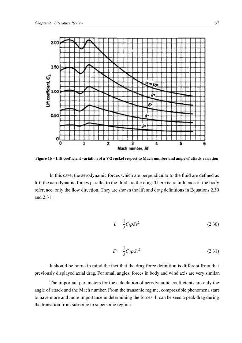
One can also use the experimental method to determine the curves of aerodynamiccoefficient, with their points taken from wind tunnel experiments. Its main advantage is the easeof implementation in this work. Figures 15 and 16 are used in the development of this work.These curves represent the German V-2 rocket were taken from Sutton (1958).

Figure 15 – Drag coefficient variation of a V-2 rocket respect to Mach number and angle of attack variation


Figure 16 – Lift coefficient variation of a V-2 rocket respect to Mach number and angle of attack variation

In this case, the aerodynamic forces which are perpendicular to the fluid are defined aslift; the aerodynamic forces parallel to the fluid are the drag. There is no influence of the bodyreference, only the flow direction. They are shown the lift and drag definitions in Equations 2.30and 2.31.

L =12

ClρSv2 (2.30)

D =12

CdρSv2 (2.31)

It should be borne in mind the fact that the drag force definition is different from thatpreviously displayed axial drag. For small angles, forces in body and wind axis are very similar.

The important parameters for the calculation of aerodynamic coefficients are only theangle of attack and the Mach number. From the transonic regime, compressible phenomena startto have more and more importance in determining the forces. It can be seen a peak drag duringthe transition from subsonic to supersonic regime.


2.3.2.4 Additional considerations on the forces and stability

In the design of air vehicles disturbance rejection should be taken into accoun. Theyare mainly caused by wind gusts. With the lateral forces, the vehicle starts to rotate around thecenter of gravity, changing the tilt axis in relation to the optimum, which generates lift.

The center of pressure is the point at which the resultant of aerodynamic forces actthroughout the body without creating zero momentum. Its meaning is analogous to the centerof gravity to the weight force. Therefore, as we take the weight force acting on the center ofgravity, we can take the aerodynamic forces acting on the center of pressure. Figure 17 showsthe possible cases. In the figure (a), there is the optimal case. There is a disturbance, causing theangle of attack to change. There is the rejection of the disturbance, as the aerodynamic forcescause a moment relative to the center of gravity, which creates a rotation that restores the vehicleto stable condition. This is a very positive effect, which occurs only if the center of gravity isabove the center of pressure. Otherwise there is a destabilizing force amplifying disturbancesand causes an increase of rotation angle relative to the desired axis, as seen in (b).

Figure 17 – Relationship between center of gravity and center of pressure on vehicle stability. In (a) there isa case with a center of pressure below the center of gravity (a stable case), in (b) center of

pressure above center of gravity (an instable case)

Therefore, a careful design and placement of the center of gravity and of the center ofpressure is necessary. Most current space systems not only use aerodynamic control of stability,but also thrust vectoring, avoiding the use of aerodynamic surfaces (Taylor 2009).


2.3.3 Equations of motion

In a body considered rigid, there are six degrees of freedom, three translations and threerotations (aeroelastic phenomena will be disregarded). In Siouris (2004), there is a detailedderivation of the equations. It uses the following assumptions:

• Rigid body with constant mass;

• Symmetry with respect to roll;

• Motion equations are solved in the frame on the vehicle

• Earth is seen as spherical, with atmosphere that turns with it and has winds defined withrespect to it.

The axis are defined as shown in Figure 18.

Figure 18 – Representation of the six degrees of freedom of the vehicle

Siouris, 2004


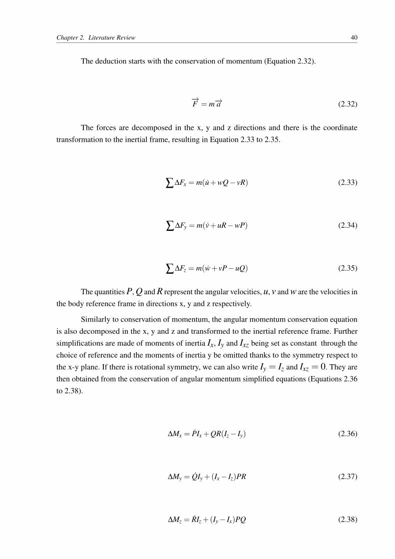
The deduction starts with the conservation of momentum (Equation 2.32).

−→F = m−→a (2.32)

The forces are decomposed in the x, y and z directions and there is the coordinatetransformation to the inertial frame, resulting in Equation 2.33 to 2.35.

∑∆Fx = m(u+wQ− vR) (2.33)

∑∆Fy = m(v+uR−wP) (2.34)

∑∆Fz = m(w+ vP−uQ) (2.35)

The quantities P, Q and R represent the angular velocities, u, v and w are the velocities inthe body reference frame in directions x, y and z respectively.

Similarly to conservation of momentum, the angular momentum conservation equationis also decomposed in the x, y and z and transformed to the inertial reference frame. Furthersimplifications are made of moments of inertia Ix, Iy and Ixz being set as constant through thechoice of reference and the moments of inertia y be omitted thanks to the symmetry respect tothe x-y plane. If there is rotational symmetry, we can also write Iy = Iz and Ixz = 0. They arethen obtained from the conservation of angular momentum simplified equations (Equations 2.36to 2.38).

∆Mx = PIx +QR(Iz− Iy) (2.36)

∆My = QIy +(Ix− Iz)PR (2.37)

∆Mz = RIz +(Iy− Ix)PQ (2.38)


Variables Mx, My e Mz represent the moments with respect to axes x, y and z respec-tively. In Siouris (2004) there is development of an algorithm using quaternions to solve theproblem for six degrees of freedom.

In Guglieri & Riboldi (2014) there is a breakdown in two plans: one longi-tudinaland lateral. The longitudinal, that is of most interest to this study is formed by the equationson Fx, Fz and My. The equations are divided in equilibrium and disturbance terms. The terms ofequilibrium are given in Equations 2.39 to 2.41.

Fxeq = Teqcosαt−Deq = 0 (2.39)

Fzeq = mg−Leq−Teqsinαt = 0 (2.40)

Meq = 0 (2.41)

Where αt is the angle between the x axis and the direction of thrust. The disturbanceterms are given in Equations 2.42 to 2.44.

∆Fx = mV (2.42)

∆Fz =−mVeq(Q− α) (2.43)

∆My = IyQ (2.44)

The terms of the disturbances are then linearized, forming a system of equations derivedfrom the speed and angle of attack and the first and second derivative of the pitch angle.

Both the approach shown in Guglieri & Riboldi (2014) and in Siouris (2004) are dis-cretized, very comfortable to implement algorithms. However, in this work we will use theapproach shown in Griffin & French (1991). It takes into account an upward trajectory equationmodel in a two-dimensional simplification. The assumptions made are:


• Spherical planet without rotation;

• The atmosphere follows the rotation of the planet;

• There may be misalignment between thrust and the main axis of the vehicle;

• Transients are ignored;

• Rotational effects caused by the thrust vectoring are ignored;

• Variable mass occurs as fuel burns;

• There is always enough lift to maintain the constant flight path angle.

The forces scheme is shown in Figure 19.

Figure 19 – Forces scheme for an ascending trajectory in a stationary planet

Griffin; French, 1991

Equations 2.45 to 2.48 define this model.

dVdt

=T cosαt−D

m−gsenγv (2.45)


dsdt

=Rr

V cosγv (2.46)

drdt

=dhdt

=V sinγv (2.47)

dmdt

=−m(t) (2.48)

Where s is the reach respect the surface of the planet, r is the distance between thevehicle and the center of the planet and γv is the angle between the horizon and vehicle speed.

44

3 Methodology

In this section there will be the discussion of the aspects of development and implementa-tion of the model used in this work. First, the choice of programming language will be discussed.Then the development and coupling of the models discussed in Section 2 are studied. Lastly, thedetermination of the mission will be discussed and the parameters used for simulation will beshown.

3.1 Modelica®

The choice of language and the whole implementation is designed for ease of use and tobe very flexible. This means a possibility to add other flight phases or refine models, reusingmuch of the developed work. In order to achieve these requirements, Modelica® was chosen.

Modelica Association (2016) defines the Modelica® as a non-proprietary language,object-oriented, based on equations to conveniently model complex physical systems of variouskinds. OpenModelica is a free code based on Modelica® language, designed for modeling andsimulating systems. It has features to combine models of multiple domains in the same simulation(OpenModelica 2016).

It is an acausal language, i.e., depends not only on inputs of previous times. It is primarilybased on equations, unlike more traditional languages that assign values to variables. Thus, themanipulation of equations is in charge of a solver, which symbolically manipulates the equationsto determine how the equations are solved and the system inputs and outputs. The languageprovides the possibility to also include algorithms in routine.

The language is based on simple models organized hierarchically and linked by connec-tors. From simple routines to form more complex models, which are in turn connected togetheruntil the molding is completed. There is an extensive pre-implemented standard library, whichitself enables the modeling of various phenomena. In Tiller (2001) there are many examples ofcomplex templates formed from several simple components connected properly.

This language easily handles complex physical problems, which generates great savingseffort for the especially because it avoids concerns on numerical resolution methods. Giventhese characteristics was chosen Modelica® language and open software OpenModelica forimplementing the physical model treated in this study.

3.2 Model implementation

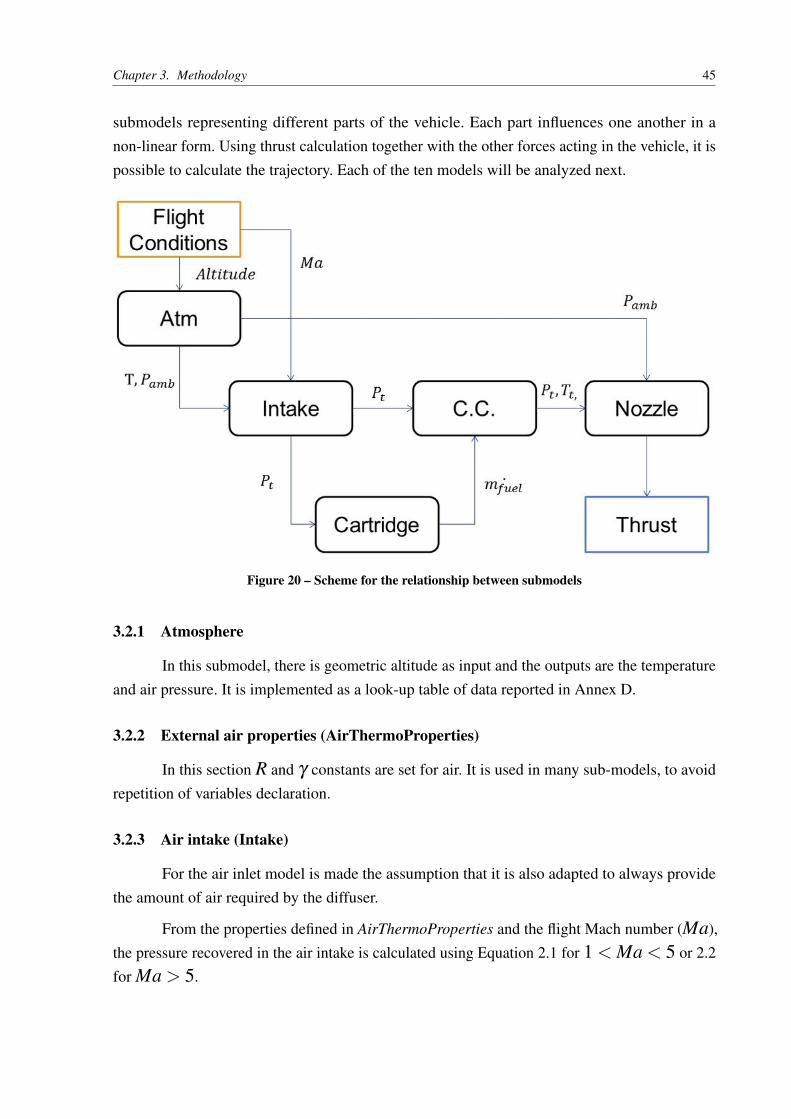
The full vehicle model is formed from the correct junction of ten submodels. Figure21 shows how thrust is calculated. Starting from flight conditions, there is the connection with

Chapter 3. Methodology 45

submodels representing different parts of the vehicle. Each part influences one another in anon-linear form. Using thrust calculation together with the other forces acting in the vehicle, it ispossible to calculate the trajectory. Each of the ten models will be analyzed next.

Figure 20 – Scheme for the relationship between submodels

3.2.1 Atmosphere

In this submodel, there is geometric altitude as input and the outputs are the temperatureand air pressure. It is implemented as a look-up table of data reported in Annex D.

3.2.2 External air properties (AirThermoProperties)

In this section R and γ constants are set for air. It is used in many sub-models, to avoidrepetition of variables declaration.

3.2.3 Air intake (Intake)

For the air inlet model is made the assumption that it is also adapted to always providethe amount of air required by the diffuser.

From the properties defined in AirThermoProperties and the flight Mach number (Ma),the pressure recovered in the air intake is calculated using Equation 2.1 for 1 < Ma < 5 or 2.2for Ma > 5.


3.2.4 Gas generator (Cartridge)

This submodel has as parameters the density of the solid propellant, the combustion area(when maintained as constant over time) and the coefficients of Vieille-Saint Robert equation,based on the work of Zadra (2016), with composition in mass of 50% HTPB, 40% AP and10% Al.This formulation was developed and tested in SPLab for the purpose of use in Ramjetpropulsion system. It has a lower oxidizer mass fraction respect to typical solid rocket motorcompositions because is a gas generator and air will be used as oxidizer in the combustionchamber. The coefficients are shown in Table 1. It‘s important to notice that a choice for acomposition does not limit the generality of the code implemented. It can be used to test theinfluence of different propellants in the final mission outcome.

Table 1 – Gas generator parameters

Ab 0.314m2

ab 0.0583(m/bar)n 0.7832

ρp 1770kg/m3

The law of Vieille-Saint Robert (Equation 2.3) is applyied, taking care to considerpressure in bar. Equation 2.4 is also used in order to obtain the mass of released fuel. Theburning area Ab is kept constant throughout the simulation. This can be made from variousgeometries, such as the rod and tube shown in Figure 9. To simulate other types of burning areavariation, it is possible to add an equation that governs the exposed surface area according tosurface regression. In this submodel there are equations governing the amount of fuel remainingin the vehicle and the quantity that has already been consumed. This is done starting from aninitial condition and a mass decrease, done by accounting for the mass of fuel released by thegrain.There is a simulation stopping condition when the fuel runs out, which returns a messageto the user if this condition is reached.

3.2.5 Combustion chamber (Combustor)

The combustion chamber has as inputs: air pressure in the air inlet, the air mass thatpasses through the diffuser and the fuel mass produced in the gas generator. The routine calculatesthe mass ratio between fuel and air. The goal is to get from this model temperature, R and γ aftercombustion, important parameters in the operation of the diffuser. For this, combustor mapsare used. In this work it’ll be used the maps from Zadra (2016), presented in Annexes A, Band C. These maps are specific for this composition, meaning that they are not valid for otherformulations, therefore it is necessary to generate new maps if a different type of mixture is used.

This model consists in three tables with two entries: pressure and ratio of mass of air andfuel. As a result of this double interpolation the three desired quantities are obtained.


3.2.6 Diffuser geometry (NozzleProperties)

In this section the diffuser geometry information are stored. It provides the value of thethroat area A∗ and of the exit area Ae, avoiding the need to initialize those parameters in everysubmodel where they appear.

3.2.7 Nozzle

It extends the NozzleProperties submodel. From the diffuser properties, altitude andcombustion gas properties, it calculates the thrust, which is one of the objectives of the work.For this, use Equations 2.7 and 2.9. In this implementation the diffuser geometry is fixed.

3.2.8 Vehicle

This is the model that makes the junction of the previous sub-models. It coordinates allthe relationship between the variables. Figure 20 shows how models are connected and whichvariables are shared by different models. Some were removed for better organization, since theyare only constant declarations (such as NozzleProperties). It is inside this model where thereis the call for the function that solves the nonlinear equation of Mach at exit section for anisentropic flow with varying area (Equation 2.8). It returns thrust value produced at a specificmoment, given the flight conditions.

3.2.9 Aerodynamic forces (AeroForces)

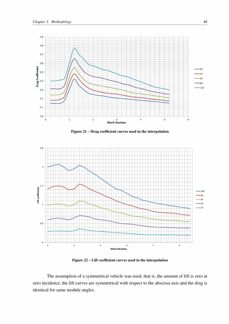
This sub-model has as inputs the angle of attack and flight Mach number. As output, itgives the values of the lift and drag coefficients. For this, it interpolates a table generated fromthe data obtained from Sutton (1958) on the V2 rocket, as discussed in section 2.3.2.3.

In Figure 21 are shown the points used to interpolate the values of drag coefficient andFigure 22, the lift coefficient.


Figure 21 – Drag coefficient curves used in the interpolation

Figure 22 – Lift coefficient curves used in the interpolation

The assumption of a symmetrical vehicle was used, that is, the amount of lift is zero atzero incidence, the lift curves are symmetrical with respect to the abscissa axis and the drag isidentical for same module angles.


The implementation of the model is done by using a double table similar to that used inthe combustor. A table is used for the lift coefficient and drag to one, both of which have the firstline with the angle indicators and the first column to the Mach indicators.

If it’s wanted to change the drag and lift curves, it’s only necessary to change the valuesin the table, always taking care to keep the angle constant in the columns and the number ofMach as rows.

3.2.10 Trajectory calculation (Trajectory)

This is the model that should be run to get the desired results. It calculates the forcesof the vehicle and the aerodynamic forces, as well as information about the properties of air ininstant flight conditions. The code calculates the trajectory by integrating Equations 2.45 to 2.48.It has the hypotheses presented in section 2.3.3. Moreover, it presents the case of:

• Variable gravity acceleration;

• Constant flightpath angle;

• Angle of attack always null.

The null angle of attack creates a null support, thanks to the vehicle symmetry hypothesis.For the analysis of the case proposed by this work, however, this will not be a problem becauseyou want to be given priority as the vehicle behaves in a trajectory with constant angle.

This model is responsible for setting the initial conditions of flight, such as speed andaltitude and vehicle configurations: total mass, fuel mass, front area to be used in the calculationof aerodynamic forces and flight angle. It’s possible to specify a misalignment angle betweenthe vehicle and the thrust if necessary, with a degree of flexibility if one wants to study how thethrust vector influences the trajectory.

The code starts with the definition of variables and initial values of the trajectory andmass fuel. Air constants are defined, as is the earth radius. They are also defined the front areavalues, the angle of attack, angle between thrust and the vehicle and the angle of trajectory. Thevalues of the aerodynamic forces are calculated, the weather conditions and the thrust producedin the instant conditions. It implemented the acceleration model of variable gravity and theequations of the trajectory and scope. It then proceeds to the integration of Equations 2.45 to2.48. The integration is done by a Dassl method, which stands for Diferential/Algebraic SystemSolver. It offers the possibility to solve ODE systems in which is difficult or impractical to writethem in the standard form y′ = f (t,y) (Petzold 1982). In practice, it solves most DAEs andODEs, even if it requires a relatively large number of steps (Liu et al. 2010). The tolerance wasset for 10−10, with recording time interval equal to 0.0005 s.


A trigger was added to end the simulation if the altitude is less than zero, if the thrustis excessive or if the ratio of the masses of air and fuel is lower then 4.1, considered as theminimum in order to have a combustion. Another condition verified is if the fuel ends up in thesolid fuel grain submodel. All of these conditions return a message to the user showing which ofthese conditions has been reached.

3.3 Initial-value and parameters problem

The mathematical problem consist of an initial-value ODE equation system. That is,proper initial conditions should be implemented. In particular, the following initializations shouldbe given: initial altitude, velocity and flight path angle.

The release altitude must be within the operating ceiling of combat aircraft. It was takenas an example the Boeing F-15, representing the fourth generation of fighter aircraft. Accordingto Boeing (2016), it has a service ceiling of 70,000 feet (21,336 m) and maximum Mach 2.5. Thisvalue is a maximum initial height, which is observed with certain clearance in all simulations,since the operation of Ramjet is very impaired by the lower air density at high altitude due tolow pressure in the interior of the vehicle if the number of Mach is not high enough.

The determination of the mission is based on studies of Socher & Gany (2008). The massof the vehicle used by them is 3,200 kg, initial Mach is 1.6 and altitude is of 47,000 feet (about14 km) and a flight angle of 16º. The initial conditions used in this study were initial velocityequal to Mach 2 and initial altitude of 14 km. This condition is still within the possibilities offighter aircraft and provides good compression given the speed. The altitude was chosen so as toreduce the mechanical stresses caused by high dynamic pressures that would be found at loweraltitudes. The flight angle was set for 9º.

The front area was determined based on missiles with mass similar to the vehicle underconsideration. These conditions are sufficient to launch a small satellite mass of about 75 kg toLEO orbit, with help from other stage rocket with solid fuel. This means acceleration to a Machhigher than 3.5 and a peak altitude of 50 km.

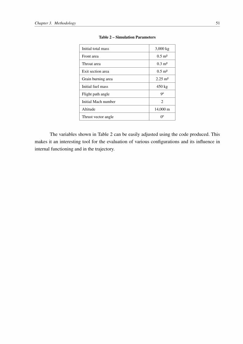
The simulation done in this work has the parameters shown in Table 2.


Table 2 – Simulation Parameters

Initial total mass 3,000 kg

Front area 0.5 m²

Throat area 0.3 m²

Exit section area 0.5 m²

Grain burning area 2.25 m²

Initial fuel mass 450 kg

Flight path angle 9º

Initial Mach number 2

Altitude 14,000 m

Thrust vector angle 0º

The variables shown in Table 2 can be easily adjusted using the code produced. Thismakes it an interesting tool for the evaluation of various configurations and its influence ininternal functioning and in the trajectory.

52

4 Results

This part is divided into three sections: the first is the simulation with the parametersdescribed in Table 2; the second is a sensitivity analysis of the most important parameters and thethird is a discussion based on the outputs. In all simulations the flight path angle is kept constantthroughout the simulation.

4.1 Scenario 1

The parameters listed in Table 2 were chosen so that the Mach number and altitude couldbe achieved while respecting the limits of the internal operation of the vehicle. This section willbe divided into two, the first being to study the evolution of the trajectory and the second to studythe evolution in time of the internal operation of the vehicle.

4.1.1 Trajectory

The simulation was performed using a maximum simulation time of 400 seconds. Thefinal simulation time was, however, 225.5 s due to the fact that oxidizer to fuel ratio reachedthe lower limit value of 4.1, which was considered the minimum for which there is combustion.This is a parameter that can be changed in the declarations of Trajectory Model. At that moment,approximately 27.5 kg of fuel remained in the vehicle ie 422.5 kg had been consumed and thefinal weight of the vehicle was 2577.5 kilograms.

Figure 23 shows the evolution of altitude respect to time. The final altitude is approxi-mately 50.1 kilometers, as established in mission requirements.

Figure 23 – Evolution of altitude in time for Scenario 1

Chapter 4. Results 53

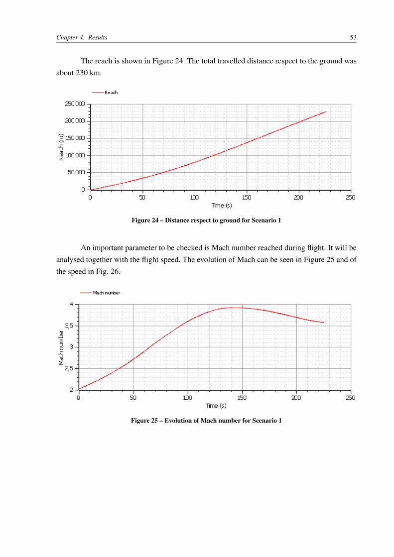
The reach is shown in Figure 24. The total travelled distance respect to the ground wasabout 230 km.

Figure 24 – Distance respect to ground for Scenario 1

An important parameter to be checked is Mach number reached during flight. It will beanalysed together with the flight speed. The evolution of Mach can be seen in Figure 25 and ofthe speed in Fig. 26.

Figure 25 – Evolution of Mach number for Scenario 1


Figure 26 – Evolution of velocity for Scenario 1

Flight Mach in the end of the simulation is 3.6, with a peak of 3.9 and the speed of about1,180 m/s (with a peak slightly above 1,220 m/s). These figures also show accordance to therequirements to start the rocket propelled phase. The progress of Mach may not perfectly equalto the speed because the former parameter depends on local atmospheric temperature. In a casewhere there is a reduction of this temperature, it is possible to have a variation in the speed ofsound large enough to influence the Mach number.

Next there will be the analysis of the forces acting on the vehicle‘s longitudinal direction.They are: drag, thrust and longitudinal component of weight, thanks to the slope of the path. Thethree forces are shown in Figure 27.

Figure 27 – Evolution of forces acting in the vehicle for Scenario 1

It can be seen in up to approximately 160 s that the thrust is greater than the sum of thedrag and weight forces. This translates into acceleration. Making a parallel with Figure 26, it is


clear that it is at that time interval when the speed increases.

The thrust force is discussed in detail in the section on the internal operation of thevehicle.

The weight in the longitudinal direction is given by Equation 4.1.

Plong = m g cosγ (4.1)

The variation of this force can be caused by variation of mass, of acceleration due togravity change or of the angle with respect to the horizon. In the present study, flight path angleis fixed, but the acceleration of gravity and mass vary. The acceleration of gravity moves froma value of 9.76 m/s at the initial time to approximately 9.65 m/s. This represents a maximumdifference of about 1% respect to the value of gravity at tedhe Earth’s surface, being a secondaryfactor in the analysis of this force.

The main factor of the variation of this force is the weight variation caused by the releaseof fuel, as can be seen in Figure 28. Weight projected in the longitudinal direction varies fromapproximately 4,580 N at the beginning to 3,890N at the end, a decrease of about 15%.

More details about the fuel consumption will be addressed in the internal operationsection.

Figure 28 – Mass variation for Scenario 1

Still in Figure 27 it is possible to see the variation in drag force. It is defined by Equation2.31, showing the variables that drag depends on. With the constant null angle of attack, the dragdepends on the square of speed and air density. Figure 29 shows how the density of the externalair varies.


Figure 29 – Atmospheric air density variation for Scenario 1

Comparing the change in velocity (Figure 26), density (Figure 29) and drag (Figure 27),it is clear that the effect of reducing the density caused by the altitude is dominant respect to theincrease of speed. At the end of the simulation, density is so low that the drag values are lessthan 200 N, against nearly 10,000 N at the beginning.

4.1.2 Internal operation

This section will analyze the parameters that generate the thrust profile found during thetrajectory. Unlike the case of the rockets, ramjets flight conditions have great influence on thegenerated thrust force.

Figure 30 shows the thrust behavior during simulation. This chart will be the startingpoint for all analysis in this section.

Figure 30 – Evolution of thrust for Scenario 1

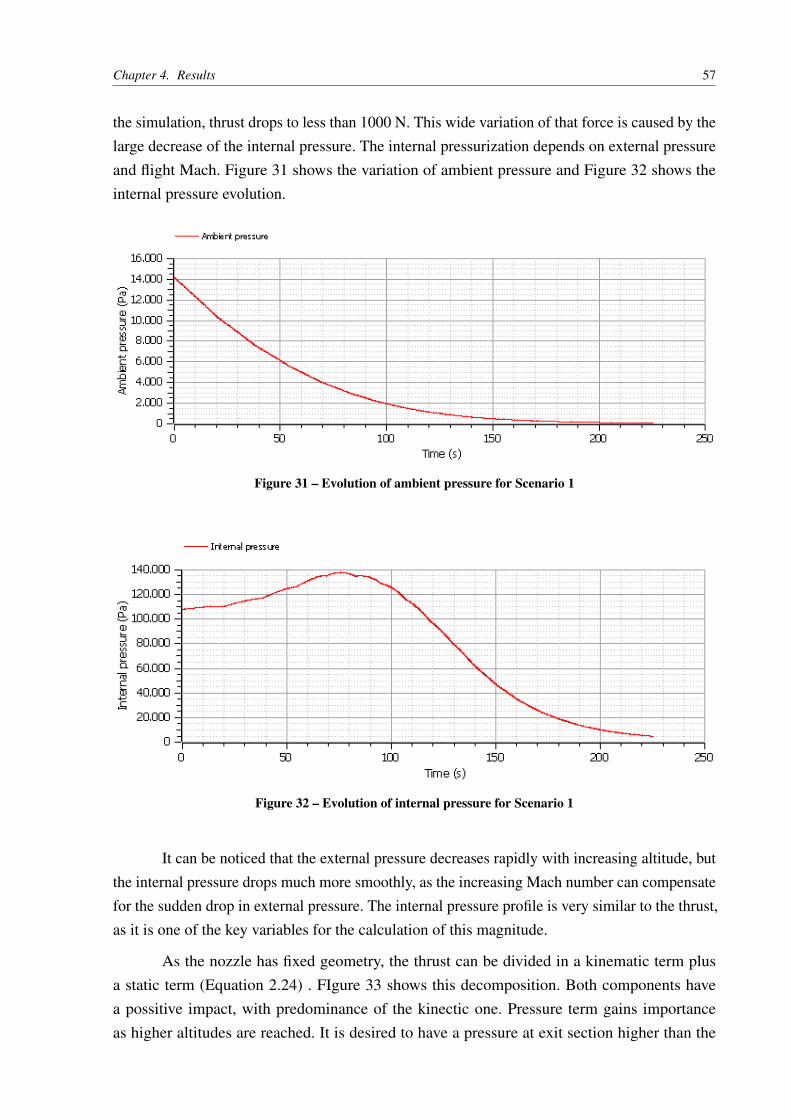
At instant zero, thrust is 23,500 N, there is a peak of 26,500 N at 63 s and, at the end of


the simulation, thrust drops to less than 1000 N. This wide variation of that force is caused by thelarge decrease of the internal pressure. The internal pressurization depends on external pressureand flight Mach. Figure 31 shows the variation of ambient pressure and Figure 32 shows theinternal pressure evolution.

Figure 31 – Evolution of ambient pressure for Scenario 1

Figure 32 – Evolution of internal pressure for Scenario 1

It can be noticed that the external pressure decreases rapidly with increasing altitude, butthe internal pressure drops much more smoothly, as the increasing Mach number can compensatefor the sudden drop in external pressure. The internal pressure profile is very similar to the thrust,as it is one of the key variables for the calculation of this magnitude.

As the nozzle has fixed geometry, the thrust can be divided in a kinematic term plusa static term (Equation 2.24) . FIgure 33 shows this decomposition. Both components havea possitive impact, with predominance of the kinectic one. Pressure term gains importanceas higher altitudes are reached. It is desired to have a pressure at exit section higher than the


atmospheric because it avoids problems with shocks inside the nozzle. This is the case in Scenario1, as thrust has a positive pressure term and the pressure profiles don‘t cross, as seen in Figure34.

Figure 33 – Thrust decomposition for Scenario 1

Figure 34 – Comparison of jet exit section and ambient pressures for Scenario 1

The next step is the analysis of the mass flows. Figure 35 shows the behavior of air,propellant and total mass flows.


Figure 35 – Variation of air, fuel and total mass flows for Scenario 1

The mass flow is defined by nozzle geometry. It can be noticed that this variable also hasthe same behavior as thrust. The specific impulse can be retrieved from the information of thrustand mass flow. Its evolution in time is shown in Figure 36.

Figure 36 – Specific impulse variation for Scenario 1

It is possible to recover the total mass of fuel burned by integrating fuel mass flow overtime. Figure 37 shows the reduction of the fuel mass. There is a small reserve of unburned fuelat the end of simulation.


Figure 37 – Fuel mass variation for Scenario 1

Figure 38 illustrates how the mass ratio of air and fuel is maintained within acceptableranges until it reaches a condition for simulation ending, when this ratio achieves a minimumvalue.

Figure 38 – Air to fuel ratio variation for Scenario 1

The values of the pressure in the combustion chamber and the ratio of the masses of airand fuel determine the burning conditions. Figure 39 shows the evolution of temperature insidecombustion chamber. The values remain fairly stable during half of the firing time, in a valueof about 2,070 K and after increases to a maximum of 2,450 K, still within the tolerable rangeconsidering the materials generally used in combustion chambers.


Figure 39 – Evolution of combustion chamber temperature for Scenario 1

It’s also possible to check the value of the Mach at the nozzle. It should be sonic andshould have a jet velocity greater than the vehicle speed in order to generate thrust. Figure 40shows the comparison between the flight and diffuser jet Mach numbers.

Figure 40 – Jet and flight Mach numbers comparison for Scenario 1

The flow is always sonic, allowing the correct functioning of the converging-divergingnozzle, but the flight Mach number is greater than the Mach number of jet at the exit . It is thennecessary to check that the jet velocity is greater than the flight speed, in order to have a positivecontribution of kinectic term of thrust. A direct correlation between Mach and velocity sholdnot be done in this case because the Mach is a local magnitude which depends also on the fluidand its temperature. There are differences between constants of gases from combustion andatmospheric air, and a great difference in temperatures. The comparison of the temperatures isshown in Figure 41.


Figure 41 – Jet and external air temperature comparison for Scenario 1

From this information it is possible to calculate the speed of the jet. It is shown in Figure42. Note that it is always higher than the speed of the jet, meaning that kinematic term has alwaysa positive contribution to the thrust.

Figure 42 – Jet and flight velocities comparison for Scenario 1

4.2 Sensitivity analysis

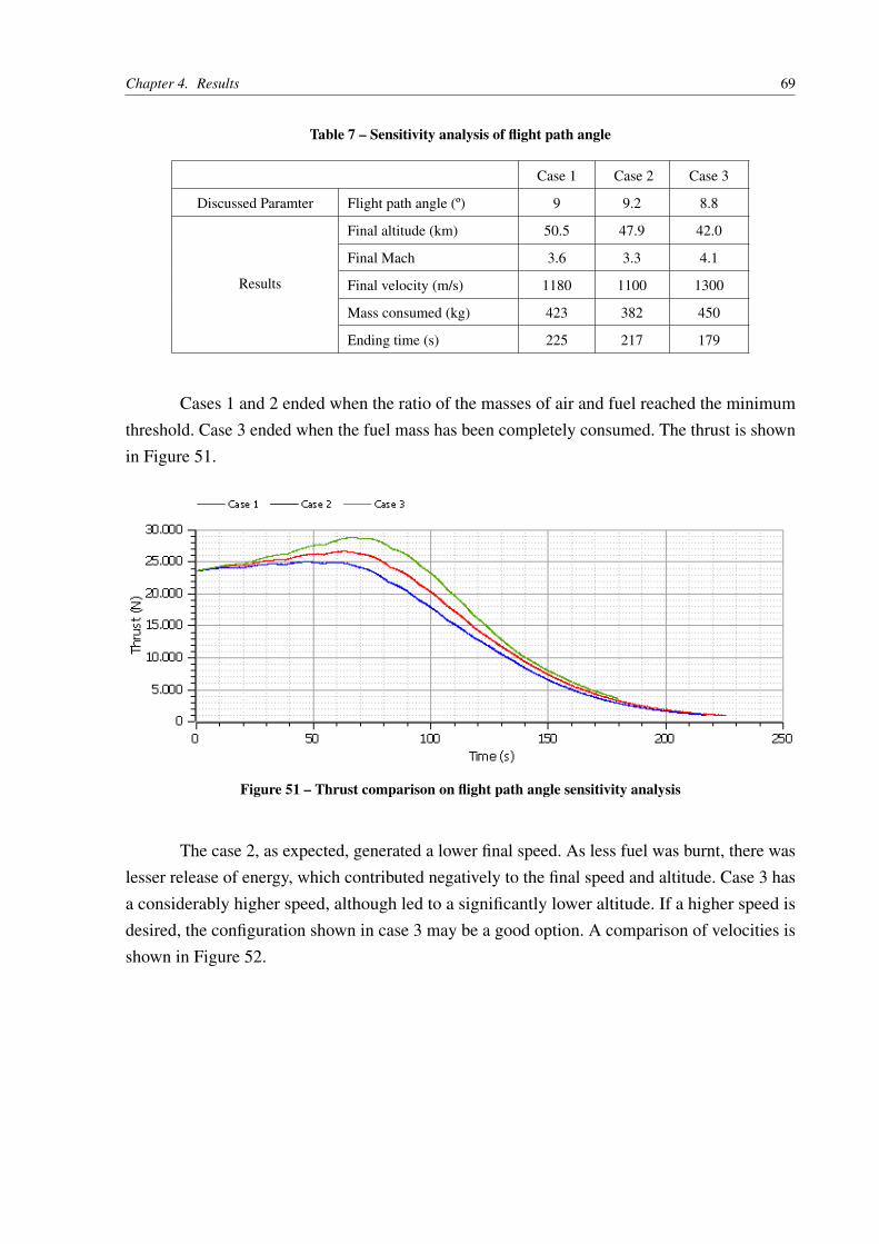
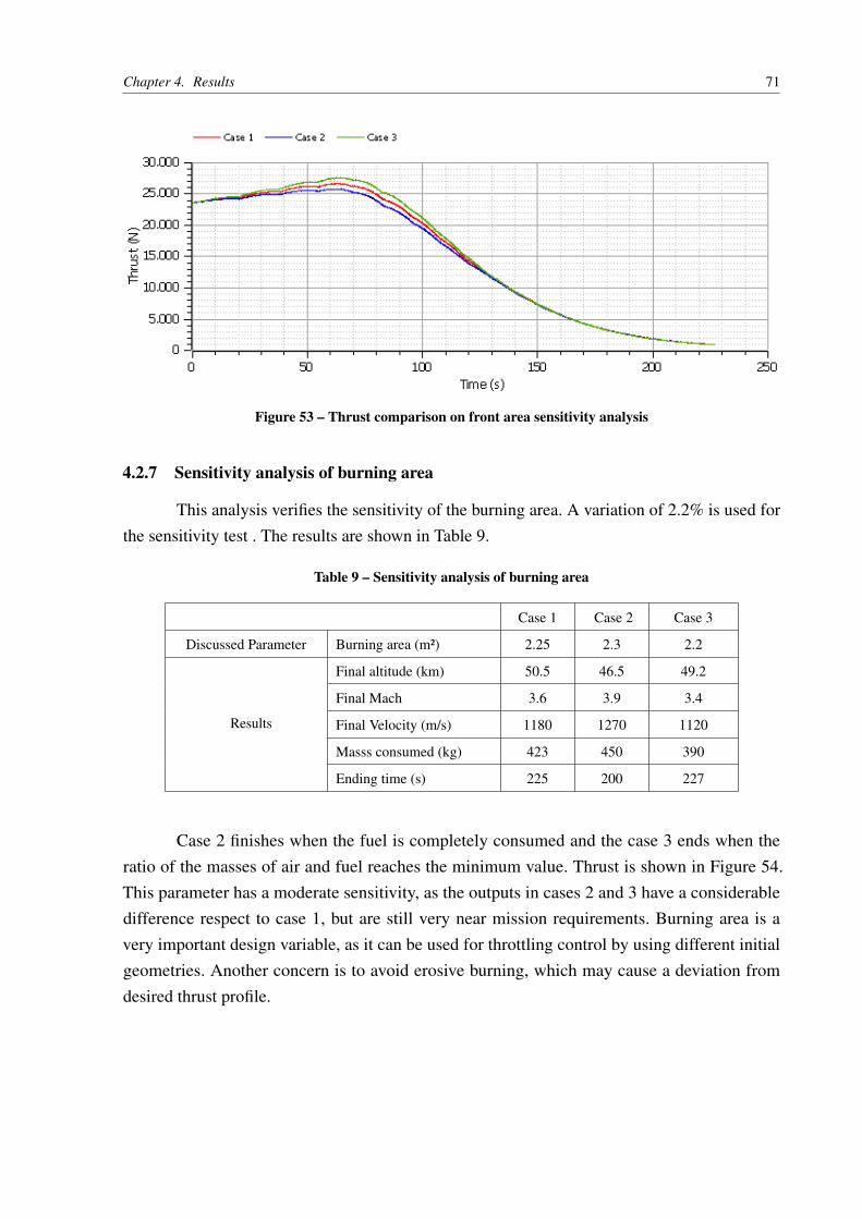
In this section there will be the study of the influence of various parameters on missionaccomplishment. In all cases there will be a comparison of the case shown in section 4.1 withtwo changes of the parameter studied. This analysis will use the same model and assumptions asScenario 1. The goal is to understand what parameters are more sensitive. Changes will be madeto the initial mass, throat area, initial altitude, initial velocity, flight angle, vehicle front area,solid fuel grain burning area and parameters of Vieillie-Saint Robert law. A brief explanation ofeach result, focusing on some of the quantities will be provided. It must be remarked that thosevariables are closely correlated and hardly a single factor is responsible for the results obtained.


Additionally, in Scenario 1 a compromise solutionis found, which means that slightly differentconfigurations can be more suitable for different mission designs.

4.2.1 Sensitivity analysis of the initial mass

The payload mass was varied by 50 kg for each case, which corresponds to approximately1.7% respect to total mass. The results are presented in Table 3.

Table 3 – Sensitivity analysis of the initial mass

Case 1 Case 2 Case 3

Discussed Parameter Initial mass (kg) 3000 3050 2950

Result

Final altitude (km) 50.5 48.4 50.5

Final Mach 3.6 3.4 3.8

Final velocity (m/s) 1180 1120 1250

Mass consumed (kg) 423 397 450

Ending time (s) 225 223 219

Cases 1 and 2 were terminated by oxidizing fuel ratio having reached the lower limit. Incase 3 the fuel was over.

As expected, less mass led to a case with a greater final velocity, which is beneficialto the mission. The mass increase, on the other hand, resulted in a lower speed and altitude asit reached the threshold of low air to fuel ratio too soon, leaving an excessive amount of fuelunburnt. Figure 43 shows the comparison of the produced thrust in all three cases. A smallervelocity at the beginning of the flight led to a smaller compression, which meant less thrust,which, together the larger component of weight in longitudinal direction, resulted in lower finalvelocity. This close relation between internal pressure and thrust can be seen by comparingFigures 43 and 44.


Figure 43 – Thrust comparison on initial mass analysis

Figure 44 – Internal pressure comparison on initial mass analysis

4.2.2 Sensitivity analysis of throat area

For this study, the throat area was changed to 1% in relation to the value of Case 1. Theresults are shown in Table 4.

Table 4 – Sensitivity analysis of throat area


Discussed Parameter Throat area (m²) 0.3 0.31 0.29

Results







Cases 1 and 3 completed by the ratio of oxidizer mass and fuel have reached the lowerlimit, in case 2 the fuel was over. The evolution of thrust can be seen in Figure 45.

Figure 45 – Thrust comparison on throat area sensitivity analysis

In case 2 burning occurs very rapidly. This configuration reaches a higher altitude andvelocity in less time than case 1. It is an advantageous configuration, but the designer has have inmind that this can lead to excessive structural stress.

In case 3 thrust is decreased respect to case 2 due to lower mass flow. With lowerthrust there is less compression, preventing the thrust increase. Decreased air flow also favorsair to fuel mass ratio to reach the bottom limit faster, which leads to an early condition ofcombustion ending. Figure 46 shows the evolution of the mass flow passing through the throat.

Figure 46 – Mass flow comparison on throat area sensitivity analysis

It can be concluded that this parameter is fairly sensible, since there is an importan


difference on thrust profiles from one case to the other .

4.2.3 Sensitivity analysis of the initial altitude

The variation studied in this section will be 300 m (approximately 1000 ft) in the initialaltitude, about 2.2% of the initial altitude. Table 5 shows the results.

Table 5 – Sensitivity analysis of the initial altitude


Discussed Parameter Initial altitude (m) 14000 14300 13700

Results






Cases 1 and 2 ended when the mass ratio of air and fuel has reached the minimum value;case 3 ended when the fuel was over. The thrust profile can be seen in Figure 47.

Figure 47 – Thrust comparison on initial altitude sensitivity analysis

In case 2 the thrust was significantly less than case 1 and case 3 produced a combustionof all fuel mass in a small time interval. This sensitivity occurs mainly due to rapid change inpressure from atmospheric air at this altitude, as shown in Figure 48. This causes two maineffects: a change in the compression and therefore of the thrust and a drag increase, whichdecreases speed and consequently also influences thrust indirecty. Initial altitude can be thusconsidered as a sensitive parameter.


Figure 48 – Pressure profile respect to altitude

4.2.4 Sensitivity analysis of the initial velocity

Parameters of sensitivity to the variation of initial velocity were studied. A change of 2%was taken in each of the cases studied. The result can be seen in Table 6.

Table 6 – Sensitivity analysis of the initial velocity


Discussed Parameter Initial velocity (m/s) 600 612 588

Results






Cases 1 and 3 ended when the mass ratio of air and fuel had reached the minimum value,while the case 2 ended when all mass of fuel was burnt. The thrust profile can be seen in Figure49.


Figure 49 – Thrust comparison on initial velocity sensitivity analysis

The difference in initial speed was sufficient to cause a different behavior between thecases. A higher speed allowed greater compression from the start, which generated a higherthrust and led to a rapid burning, while a lower speed has the opposite effect. This influence canbe seen by comparing Figure 49 and 50. As there is a quite different output for each case studied,it is possible to conclude that this is a sensitive parameter.

Figure 50 – Internal pressure comparison on initial velocity sensitivity analysis

4.2.5 Sensitivity analysis of flight path angle

The angle sensitivity analysis will be performed by changing the angle of 0.2° respect tothe base value, a difference of about 2.2%. The results are shown in Table 7.


Table 7 – Sensitivity analysis of flight path angle


Discussed Paramter Flight path angle (º) 9 9.2 8.8

Results






Cases 1 and 2 ended when the ratio of the masses of air and fuel reached the minimumthreshold. Case 3 ended when the fuel mass has been completely consumed. The thrust is shownin Figure 51.

Figure 51 – Thrust comparison on flight path angle sensitivity analysis

The case 2, as expected, generated a lower final speed. As less fuel was burnt, there waslesser release of energy, which contributed negatively to the final speed and altitude. Case 3 hasa considerably higher speed, although led to a significantly lower altitude. If a higher speed isdesired, the configuration shown in case 3 may be a good option. A comparison of velocities isshown in Figure 52.


Figure 52 – Velocity comparison on flight path angle sensitivity analysis

4.2.6 Sensitivity analysis of vehicle front area

The final area is an important parameter for calculating the drag. A study was done withthe variation of 2% of this parameter. The results are shown in Table 8.

Table 8 – Sensitivity analysis of vehicle frontarea


Discussed parameter Front area (m²) 0.5 0.51 0.49

Results






All cases stopped when the oxidizer to fuel mas ratio reached the minimum. In Figure53 the variation of thrust is shown. As expected, a better performance was achieved by reducingthe front area, consequently diminishing drag losses. All configurations had a very similar output,which demonstrates that this variable has low sensibility.


Figure 53 – Thrust comparison on front area sensitivity analysis

4.2.7 Sensitivity analysis of burning area

This analysis verifies the sensitivity of the burning area. A variation of 2.2% is used forthe sensitivity test . The results are shown in Table 9.

Table 9 – Sensitivity analysis of burning area


Discussed Parameter Burning area (m²) 2.25 2.3 2.2

Results



Final Velocity (m/s) 1180 1270 1120

Masss consumed (kg) 423 450 390


Case 2 finishes when the fuel is completely consumed and the case 3 ends when theratio of the masses of air and fuel reaches the minimum value. Thrust is shown in Figure 54.This parameter has a moderate sensitivity, as the outputs in cases 2 and 3 have a considerabledifference respect to case 1, but are still very near mission requirements. Burning area is avery important design variable, as it can be used for throttling control by using different initialgeometries. Another concern is to avoid erosive burning, which may cause a deviation fromdesired thrust profile.


Figure 54 – Thrust comparison on burning area sensitivity analysis

4.2.8 Sensitivity analysis of Vieille’s law constant

In this section, the sensitivity analysis was made with the variation of 2.5% in the constantof Vieille‘s law. The results are compiled in Table 10.

Table 10 – Sensitivity analysis of fuel release law constant


Discussed Parameter Law constant 0.0583 0.0597 0.0568

Results




Consumed mass (kg) 423 450 386


The simulation of the case 2 ended when the fuel was all released. In case 3 the simulationwas stopped because of the ratio of mass of air and fuel, which reached the lower limit. In Figure55 the progress of thrust in those three cases is presented. With a higher constant, air to massfuel ratio was kept lower, which increased combustion chamber temperature and had a positiveeffect on thrust. This can be seen in Figure 56 and 57.


Figure 55 – Thrust comparison on Vieille’s law constant sensitivity analysis

Figure 56 – Air to fuel ratio comparison on Vieille‘s law constant sensitivity analysis


Figure 57 – Combustion chamber temperature comparison on Vieille’s law constant sensitivity analysis

4.2.9 Sensitivity analysis of Vieille‘s law exponent

For the analysis of Vieille’s law exponent there was a variation of 2.5%. The resultsfound are summarized in the Table 11.

Table 11 – Sensitivity analysis of the fuel releaselaw exponent


Discussed parameter Law exponent 0.7832 0.8223 0.7440

Results




Consumed mass (kg) 423 433 413


All cases ended when the oxidizer to fuel ratio having reached the minimum acceptable.The thrust profiles are quite similar in all cases, being hardly distinguishable as shown in Figure58. Even with very similar profiles, there is a significant change in the final altitude. It happensbecause the combustion ends at different times for each case. The case with higher exponentcould keep the air to fuel ratio a longer time inside the burning envelope, allowing more fuel tobe burnt and therefore more energy to be released (see Figure 59).


Figure 58 – Thrust comparison of Vieille‘s law exponent sensitivity analysis

Figure 59 – Ait to fuel ratio comparison on Vieille’s law exponent sensitivity analysis

4.3 Discussion of results

The configuration presented in Scenario 1 had a satisfactory fulfillment of missionrequirements. It increased final velocity from 600 m/s to about 1200 m/s, while changing the alti-tude from 14 km to 50 km in 225 s. Its main advantage when comparing to current launchingmethods is the use of air as oxidant, which translates into higher specific impulse. In Scenario 1there was a peak of specific impulse of almost 1900 s, whereas chemical rockets usually havethis parameter around 300 s for solid rocket motors or 400 s for liquid bipropellants (Sutton &Biblarz 2010). This means a great weight saving by not carrying oxidants for this flight phase.It is worth to mention that the configuration found in Scenario 1 is a compromise solution thatstrongly depends on the mission requirements. This is exemplified by some results on sensibilityanalysis, which had a better performance in some aspects when compared to Scenario 1. For


better results it is recommended a joint development and optimization of Ramjet phase togetherwith the pure rocket phase.

The model presented in this work indicated that there is a relative stability in thistechnology (as no sensitivity analysis led to an unstable behavior), although the controllabilitymay be an issue because solid grain gas generators aren‘t as throttleable as liquid systems. Also,this system is prone to amplify disturbances, as a decrease in velocity means less compressionand therefore less throttle, which will prevent velocity from increasing. No variable was foundto be completely insensitive. Initial velocity, initial altitude and flight path angle were the mostsensitive. In order to overcome this problem it is desirable to have control over as many variablesas possible. This can be done by designing initial grain geometry for better performance indifferent phases or by trajectory optimization and control (by using aerodynamic actuators orthrust vectoring).

This technology presents many influencing variables that can be changed to fulfill verydifferent mission requirements, which means a very flexible range of uses for this general design.

77

5 Conclusions

The objective of this work is to build a tool that can assist in the early stages of a realproject of small satellite launcher from supersonic aircraft, which has the first flight phaseas Ramjet and later a stage as conventional rocket to get to LEO. This tool was producedsuccessfully and allows the user to change various parameters and analyze with great ease. Themain parameters are:

• Total mass of the vehicle;

• Throat area of the convergent-divergent nozzle;

• Exit area of the convergent-divergent nozzle;

• Initial altitude;

• Initial velocity;

• Flight angle;

• Frontal area of the vehicle;

• Embedded fuel mass;

• Burning area of a solid fuel grain;

• Parameters of the law of Vieille-Saint Venant, governing the release of fuel from solid fuelgrain.

A configuration was found to comply with the objectives of the mission and allow asecond stage to take the satellite to the position necessary to enter the LEO. This shows that theproject is feasible from a theoretical point of view and can prove to be a valuable solution forsmall satellite access problem to LEO.

A sensitivity analysis was made showing how the mass parameters, trajectory angle,initial altitude and speed conditions are very sensitive. This is because there is only controllingthe flow of air from the throat area and the angle of trajectory. For a more robust operation,more control is required, such as trajectories optimized and controlled (by thrust vectoringor aerodynamic actuators) and grain geometries which lead to more stable conditions. The

Chapter 5. Conclusions 78

parameters of linked to the chemical composition of the propellant had a lower sensitivity. Theburning area also showed low sensitivity, an important factor since in real cases there may beerosive burning, causing combustion irregularities.

The next steps include the refinement of the trajectory model, perhaps including actuatorsand vector thrust. It is also advised that the implementation of a more sophisticated model to theair inlet. Another important step would be to make a study of the mission design, including anextensive analysis of the variables using the tool developed in this work, maybe coupling withthe studies of rocket phase.

79

References

Athawale, B., Asthana, S. & Singh, H. (1994), Metallised Fuel-rich Propellants for Solid Rocket

Ramjet -A Review, Defence Science Journal 44(4), 269 – 278.

Boeing (2016), F-15 Technical Specifications.

URL: http://www.boeing.com/defense/f-15-strike-eagle/

Bray, K. & Appleton, J. (1963), Atomic Recombination in Nozzles: Methods of Analysis for

Flows with Complicated Chemistry, Technical Report 0636, Ministry of Aviation, Aeronautical

Research Council, London.

de Morais, A. M. F. (2000), Caracterização do Comportamento Mecânico do Propelente Sólido

Compósito Como Material Estrutural, PhD thesis, Universidade Estadual de Campinas, Campinas

- São Paulo.

Farokhi, S. (2009), Aircraft Propulsion, 2 edn, Wiley, New York.

Fleeman, E. L. (2001), Tactical Missile Design, AIAA Educational Series, Reston, VA.

Fry, R. S. (2004), A Century of Ramjet Propulsion Technology Evolution, Journal of Propulsion

and Power 20(1), 27 – 58.

Griffin, M. D. & French, J. R. (1991), Space Vehicle Design, AIAA Education series, 1 edn,

American Institute of Aeronautics and Astronautics, Washington, D.C.

Guglieri, G. & Riboldi, C. E. D. (2014), Introduction to Flight Dynamics, 1 edn, Celid, Torino,

Italy.

Javed, A. & Chakraborty, D. (2015), Universal erosive burning model performance for solid

rocket motor internal ballistics, Aerospace Science and Technology 45, 150 – 153.

Jr., R. E. W. & Strauss, R. F. (1960), Fundamentals of Rocket Propulsion, Reinhold Publishing

Corporation. Reinhold Space Technology Series.

Levin, V. M. (2010), Problems of Implementing Ramjet Operation, Combustion, Explosion,

and Shock Waves 46(4), 408 – 417.

Liu, L., Felgner, F. & Frey, G. (2010), Comparison of 4 Numerical Solvers for Stiff and Hy-

brid Systems Simulation , in ‘IEEE 15th Conference on Emerging Technologies & Factory

Automation (ETFA 2010)’, IEEE, Bilbao.

Mignot, N. (1963), Le guidage des fusées, Éditions Fayard, Paris.

http://www.boeing.com/defense/f-15-strike-eagle/

References 80

Modelica Association (2016), Modelica and the Modelica Association, On-line resource.

URL: https://www.modelica.org/

MUKUNDA, H. S. & PAUL, P. J. (1997), Universal Behaviour in Erosive Burning of Solid

Propellants , Combust. Flame (109), 224 – 236.

NASA (2015), Historical Studies in the Societal Impact of Spaceflight, NASA History Program

Office, Washington, D.C.

URL: http://www.nasa.gov/sites/default/files/atoms/files/historical-studies-societal-impact-

spaceflight-ebooktagged.pd f

NASA (2016), Economic Development of Low Earth Orbit, National Aeronautics and Space

Administration, Washington, DC.

URL: http://www.nasa.gov/sites/default/files/atoms/files/economic-development-of-low-earth-

orbittaggedv2.pd f

NASA, United States Air Force & United States Weather Bureau (1962), U.S. Standard Atmo-

sphere, 1962, Technical report, U.S. Government Printing Office, Washington, D.C.

URL: http://ntrs.nasa.gov/archive/nasa/casi.ntrs.nasa.gov/19630003300.pdf

Nielsen, J. N. (1960), Missile Aerodynamics, McGraw-Hill Series in Missile and Space Technol-

ogy, McGraw-Hill Book Company, New York.

Niskanen, S. (2013), OpenRocket technical documentation, Technical documentation, Open-

Rocket.

OpenModelica (2016), Modelica User Guide.

URL: https://build.openmodelica.org/Documentation/Modelica.UsersGuide.html

Park, I., Park, J. & Tahk, M. (2011), ‘Control-Oriented Model for Intake Shock Position Dynam-

ics in Ramjet Engine’, Journal of Propulsion and Power 27(2).

Petzold, L. R. (1982), A Description of DASSL: A Differential/Algebraic System Solver, in

‘IMACS World Congress’, IMACS, Montreal, Canada.

Rowell, L. F. & Korte, J. J. (2003), Launch Vehicle Design and Optimization Methods and

Priority for the Advanced Engineering Environment, NASA Langley Research Center, Hampton,

VA.

Ryan, R. S. & Townsend, J. S. (1997), Fundamentals and Issues in Launch Vehicle Design,

Journal of Spacecraft and Rockets 34(2), 192 – 198.

Siouris, G. M. (2004), Missile Guidance and Control System, 1 edn, Springer-Verlag New York.

http://www.modelica.org/

http://www.nasa.gov/sites/default/files/atoms/files/historical-studies-societal-impact-

http://www.nasa.gov/sites/default/files/atoms/files/economic-development-of-low-earth-

http://ntrs.nasa.gov/archive/nasa/casi.ntrs.nasa.gov/19630003300.pdf

References 81

Socher, A. & Gany, A. (2008), Investigation of Combined Air-breathing/Rocket Propulsion for

Air Launch of MicroSatellites from a Combat Aircraft , in ‘6th Responsive Space Conference’,

AIAA, Los Angeles, CA.

Sutton, G. P. (1958), Rocket Propulsion Elements, 2 ed. edn, Wiley, New York.

Sutton, G. P. & Biblarz, O. (2010), Rocket Propulsion Elements, 8 edn, Chichester, United

Kingdom.

Taylor, T. S. (2009), Introduction to Rocket Science and Engineering, 1 edn, CRC Press, Boca

Raton, Florida.

Tiller, M. (2001), Introduction to physical modeling with Modelica, Boston [etc.] : Kluwer.

U.S (1973), MIL-E-5007D, Military Specification: Engine, Aircraft, Turbojet And Turbofan,

General Specification For.

Yoder, D. A., Georgiadis, N. J. & O’Gara, M. R. (2008), Frozen Chemistry Effects on Nozzle

Performance Simulations, in ‘38th Fluid Dynamics Conference and Exhibit sponsored by the

American Institute of Aeronautics and Astronautics’, NASA Center for Aerospace Information,

Seattle, Washington.

Zadra, F. (2016), Gas Generating Pyrolants for Ducted Rocket Application, Master’s thesis,

Politecnico di Milano, Milan, Italy.

Zucker, R. D. & Biblarz, O. (2012), Fundamentals of Gas Dynamics, 2 edn, John Wiley & Sons,

Hoboken, New Jersey.

Annex

83

ANNEX A – Combustor map - Temperature

Fonte: SPLab - Politecnico di Milano

84

ANNEX B – Combustor map - Ideal Gas Constant


85

ANNEX C – Combustor map - Specific heat ratio


86

ANNEX D – United States Standard Atmosphere

Fonte: Faroki, S. (2009)

87

ANNEX E – Modelica Code

Listing E.1 – Código de simulação do veículo Ramjet e de sua trajetória

c l a s s GeomFixamodel I n t a k e

p a r a m e t e r Rea l A = 3 . 1 4 ;e x t e n d s GeomFixa . A i r T h e r m o P r o p e r t i e s ;Rea l Ma( min = 1) ;Rea l T ( min = 200) , P ( min = 0) , pamb ( min = 0) , rho ( min = 0) ,

a ( min = 0) , mdot ( min = 0) ;Rea l h ( min = 0) , p i d ;GeomFixa . Atmosphere atm ;

p r o t e c t e dRea l TC ;

a l g o r i t h mi f Ma < 5 t h e n

p i d := 1 − 0 .075 * (Ma − 1) ^ 1 . 3 5 ;e l s e

p i d := 800 / (Ma ^ 4 + 935) ;end i f ;

e q u a t i o nc o n n e c t ( h , atm . h ) ;c o n n e c t ( atm . T , TC) ;c o n n e c t ( atm . pamb , pamb ) ;rho = P / (R * T ) ;a = s q r t ( gamma * R * T ) ;mdot = rho * A * Ma * a ;P = p i d * pamb * (1 + Ma ^ 2 * ( gamma − 1) / 2 ) ^ ( gamma /

( gamma − 1) ) ;a l g o r i t h m

T := TC + 2 7 3 . 1 5 ;end I n t a k e ;

model Atmospherei n p u t Rea l h ;o u t p u t Rea l T ( min = 200) , pamb ( min = 0) ;

p r o t e c t e dModel ica . B locks . T a b l e s . CombiTable1Ds ICAO( t a b l e =

[−2000.000000 , 301 .200000 , 127800 .000000 ; 0 . 0 0 0 0 0 0 ,288 .100000 , 101300 .000000 ; 2000 .000000 , 275 .200000 ,7 9 5 0 0 . 0 0 0 0 0 0 ; 4000 .000000 , 262 .200000 , 6 1 6 6 0 . 0 0 0 0 0 0 ;6000 .000000 , 249 .200000 , 4 7 2 2 0 . 0 0 0 0 0 0 ; 8000 .000000 ,236 .200000 , 3 5 6 5 0 . 0 0 0 0 0 0 ; 10000 .000000 , 223 .300000 ,2 6 5 0 0 . 0 0 0 0 0 0 ; 12000 .000000 , 216 .600000 , 1 9 4 0 0 . 0 0 0 0 0 0 ;14000 .000000 , 216 .600000 , 1 4 1 7 0 . 0 0 0 0 0 0 ; 16000 .000000 ,216 .600000 , 1 0 3 5 0 . 0 0 0 0 0 0 ; 18000 .000000 , 216 .600000 ,7 5 6 5 . 0 0 0 0 0 0 ; 20000 .000000 , 216 .600000 , 5 5 2 9 . 0 0 0 0 0 0 ;22000 .000000 , 216 .600000 , 4 0 4 7 . 0 0 0 0 0 0 ; 24000 .000000 ,220 .600000 , 2 9 7 2 . 0 0 0 0 0 0 ; 26000 .000000 , 222 .500000 ,2 1 8 8 . 0 0 0 0 0 0 ; 28000 .000000 , 224 .500000 , 1 6 1 6 . 0 0 0 0 0 0 ;30000 .000000 , 226 .500000 , 1 1 9 7 . 0 0 0 0 0 0 ; 32000 .000000 ,

ANNEX E. Modelica Code 88

228 .500000 , 8 8 9 . 0 0 0 0 0 0 ; 34000 .000000 , 233 .700000 ,6 6 3 . 4 0 0 0 0 0 ; 36000 .000000 , 239 .300000 , 4 9 8 . 5 0 0 0 0 0 ;38000 .000000 , 244 .800000 , 3 7 7 . 1 0 0 0 0 0 ; 40000 .000000 ,250 .400000 , 2 8 7 . 1 0 0 0 0 0 ; 42000 .000000 , 255 .900000 ,2 2 0 . 0 0 0 0 0 0 ; 44000 .000000 , 261 .400000 , 1 6 9 . 5 0 0 0 0 0 ;46000 .000000 , 266 .900000 , 1 3 1 . 3 0 0 0 0 0 ; 48000 .000000 ,270 .600000 , 1 0 2 . 3 0 0 0 0 0 ; 50000 .000000 , 270 .600000 ,7 9 . 7 7 0 0 0 0 ; 52000 .000000 , 269 .000000 , 6 2 . 2 1 0 0 0 0 ;54000 .000000 , 263 .500000 , 4 8 . 3 3 0 0 0 0 ; 56000 .000000 ,258 .000000 , 3 7 . 3 6 0 0 0 0 ; 58000 .000000 , 252 .500000 ,2 8 . 7 2 0 0 0 0 ; 60000 .000000 , 247 .000000 , 2 1 . 9 6 0 0 0 0 ;62000 .000000 , 241 .500000 , 1 6 . 6 9 0 0 0 0 ; 64000 .000000 ,236 .000000 , 1 2 . 6 0 0 0 0 0 ; 66000 .000000 , 230 .500000 ,9 . 4 5 9 0 0 0 ; 68000 .000000 , 225 .100000 , 7 . 0 5 1 0 0 0 ;70000 .000000 , 219 .600000 , 5 . 2 2 0 0 0 0 ; 72000 .000000 ,214 .300000 , 3 . 8 3 5 0 0 0 ; 74000 .000000 , 210 .300000 ,2 . 8 0 0 0 0 0 ; 76000 .000000 , 206 .400000 , 2 . 0 3 3 0 0 0 ;78000 .000000 , 202 .500000 , 1 . 4 6 7 0 0 0 ; 80000 .000000 ,198 .600000 , 1 . 0 5 2 0 0 0 ; 82000 .000000 , 194 .700000 ,0 . 7 4 9 8 0 0 ; 84000 .000000 , 190 .800000 , 0 . 5 3 0 8 0 0 ;86000 .000000 , 186 .900000 , 0 . 3 7 3 2 0 0 ] ) ;

e q u a t i o nc o n n e c t ( h , ICAO . u ) ;ICAO . y [ 1 ] = T ;ICAO . y [ 2 ] = pamb ;

end Atmosphere ;

model Nozzlee x t e n d s GeomFixa . N o z z l e P r o p e r t i e s ;Rea l Pamb , Pe , F , Fm, Fp , mdot , rhoprod , aprod ,V;/ / Rea l Pcomb =1000000 , h =10000 , Tcomb =2200;/ / Rea l gamma = 1 . 2 5 , R= 2 8 2 . 4 ;Rea l Pcomb ( s t a r t = 100000 , min = 0) , h , Tcomb ( s t a r t = 2200 ,

min = 500 , max = 3000) ;Rea l gamma ( s t a r t = 1 . 3 , min = 1 , max = 1 . 4 ) , R( s t a r t = 282 ,

min = 200 , max = 300) ;GeomFixa . Atmosphere atm ;

e q u a t i o nc o n n e c t ( atm . h , h ) ;c o n n e c t ( atm . pamb , Pamb ) ;

Pe = Pcomb * (1 +( ( gamma − 1) / 2 ) * (Me ^ 2) ) ^ (−gamma /( gamma − 1) ) ;

a l g o r i t h m/ / Pe := Pamb ;/ / Me := s q r t (2 / ( gamma − 1) * ( ( Pe / Pcomb ) ^ ( ( 1 − gamma )

/ gamma ) − 1) ) ;/ / Ae := At / Me * ( ( gamma + 1) / 2 / (1 + ( gamma − 1) / 2 *

Me ^ 2) ) ^ (−(gamma + 1) / (2 * ( gamma − 1) ) ) ;/ / mdot := r h o p r o d * aprod * At ;

mdot := Pe * Ae * s q r t (2 * gamma / ( ( gamma − 1) * R * Tcomb ) *( ( Pcomb / Pe ) ^ ( ( gamma − 1) / gamma ) − 1) * ( Pcomb / Pe ) ^( ( gamma − 1) / gamma ) ) ;

/ / F := Pe * Ae * (2 * gamma / ( gamma − 1) * ( ( Pcomb / Pe ) ^ ( (gamma − 1) / gamma ) − 1) + 1 − Pamb / Pe ) ;


Fm := Pe * Ae * (2 * gamma / ( gamma − 1) ) * ( ( Pcomb / Pe ) ^( ( gamma − 1) / gamma ) − 1) ;

Fp := (1 − Pamb / Pe ) * Pe * Ae ;F := Fm + Fp ;V:= s q r t ( ( 2 * gamma*R*Tcomb / ( gamma−1) ) *(1−( Pe / Pcomb ) ^ ( ( gamma−1) / gamma ) ) ) ;

/ / Me:= Model ica . Math . N o n l i n e a r . s o l v e O n e N o n l i n e a r E q u a t i o n (f u n c t i o n / / GeomFixa . Me( gamma=gamma , Ae=Ae , At=At ) , 1 , 2 5 ) ;

end Nozzle ;

model A i r T h e r m o P r o p e r t i e sp a r a m e t e r Rea l R = 2 8 7 . 0 5 8 ;p a r a m e t e r Rea l gamma = 1 . 4 ;

end A i r T h e r m o P r o p e r t i e s ;

model T e s t a d o rRea l a ;a l g o r i t h m

a := SolveMe ( Ae_Me=1 ,At_Me=2 ,gamma_Me=2) ;

end T e s t a d o r ;

f u n c t i o n Me " F i n d s Mach a t t h e e x i t o f n o z z l e "e x t e n d s Model ica . Math . N o n l i n e a r . I n t e r f a c e s .

p a r t i a l S c a l a r F u n c t i o n ;i n p u t Rea l gamma , Ae , At ;

a l g o r i t h my := Ae / At − 1 / u * ( ( gamma + 1) / 2 / (1 + ( ( gamma − 1)

/ 2 ) * ( u ^ 2 ) ) ) ^ (−(gamma + 1) / (2 * ( gamma − 1) ) ) ;end Me;

model C a r t r i d g ep a r a m e t e r Rea l rhop = 1770 ;/ / Connect p . Review r e g r e s s i o n r a t e p a r a m e t e r sp a r a m e t e r Rea l Ab = 2 . 2 5 ;/ / 0 . 6 ;p a r a m e t e r Rea l n = 0 . 7 8 3 2 ;p a r a m e t e r Rea l a = 0 . 0 5 8 3 ;/ / p a r a m e t e r Rea l p r e f = 6 8 ;Rea l mdotp ;i n p u t Rea l p ;Rea l mpconsumed ( s t a r t = 0 ) ;Rea l m p t o t a l ( s t a r t = 450) ;

e q u a t i o nd e r ( mpconsumed ) = mdotp ;d e r ( m p t o t a l ) = −mdotp ;

a l g o r i t h mmdotp := rhop * Ab * a * ( p * 1e−5) ^ n * 1e−2;i f m p t o t a l < 0 t h e n

t e r m i n a t e ( " A l l f u e l has been b u r n t ! " ) ;end i f ;

end C a r t r i d g e ;


model CombustorRea l mdotp ( min = 0) , mdota ( min = 0) , mdot ( min = 0) , p t o t ,

gammaprod , Rprod , rhoprod , ap rod ;Rea l OF( min = 3) ;Rea l T ;/ / Tempera tu r eModel ica . B locks . T a b l e s . CombiTable2D Temp ( t a b l e = [ 0 . 0 0 0 0 0 0 ,

5 . 0 0 0 0 0 0 , 6 . 6 7 0 0 0 0 , 8 . 0 0 0 0 0 0 , 10 .000000 , 12 .000000 ,2 0 . 0 0 0 0 0 0 ; 40000 .000000 , 2448 .100000 , 2403 .700000 ,2291 .300000 , 2067 .300000 , 1862 .600000 , 1 3 6 5 . 7 0 0 0 0 0 ;88000 .000000 , 2477 .100000 , 2438 .800000 , 2313 .300000 ,2073 .500000 , 1864 .300000 , 1 3 6 5 . 8 0 0 0 0 0 ; 164000 .000000 ,2577 .600000 , 2534 .900000 , 2411 .300000 , 2204 .400000 ,2009 .200000 , 1 5 3 3 . 3 0 0 0 0 0 ; 192000 .000000 , 2505 .900000 ,2475 .500000 , 2327 .000000 , 2085 .400000 , 1873 .500000 ,1 3 7 5 . 0 0 0 0 0 0 ; 313000 .000000 , 2654 .800000 , 2611 .800000 ,2491 .300000 , 2293 .100000 , 2105 .400000 , 1 6 4 4 . 0 0 0 0 0 0 ;360000 .000000 , 2606 .400000 , 2571 .300000 , 2433 .800000 ,2212 .000000 , 2011 .600000 , 1 5 3 3 . 4 0 0 0 0 0 ; 562000 .000000 ,2740 .200000 , 2696 .000000 , 2581 .000000 , 2384 .000000 ,2216 .700000 , 1 7 7 3 . 1 0 0 0 0 0 ; 685000 .000000 , 2685 .000000 ,2649 .600000 , 2515 .600000 , 2302 .200000 , 2108 .600000 ,1 6 4 4 . 2 0 0 0 0 0 ; 733000 .000000 , 2589 .800000 , 2570 .200000 ,2408 .900000 , 2163 .500000 , 1953 .900000 , 1 4 6 5 . 2 0 0 0 0 0 ;787000 .000000 , 2637 .800000 , 2611 .700000 , 2461 .600000 ,2228 .800000 , 2025 .600000 , 1 5 4 7 . 5 0 0 0 0 0 ; 1231000 .000000 ,2773 .000000 , 2736 .100000 , 2608 .100000 , 2395 .000000 ,2221 .300000 , 1 7 7 3 . 5 0 0 0 0 0 ; 1499000 .000000 , 2719 .700000 ,2693 .300000 , 2547 .300000 , 2322 .900000 , 2126 .200000 ,1 6 6 1 . 8 0 0 0 0 0 ; 2694000 .000000 , 2813 .000000 , 2784 .500000 ,2645 .400000 , 2421 .100000 , 2244 .200000 , 1 7 9 6 . 2 0 0 0 0 0 ;3010000 .000000 , 2755 .700000 , 2737 .900000 , 2582 .600000 ,2339 .700000 , 2153 .700000 , 1 6 9 1 . 3 0 0 0 0 0 ; 5730000 .000000 ,2862 .200000 , 2841 .900000 , 2694 .600000 , 2463 .900000 ,2286 .300000 , 1 8 4 1 . 7 0 0 0 0 0 ; 10297000 .000000 , 2984 .000000 ,2959 .600000 , 2822 .900000 , 2607 .800000 , 2430 .300000 ,2 0 1 7 . 1 0 0 0 0 0 ] ) ;

/ / RModel ica . B locks . T a b l e s . CombiTable2D R1 ( t a b l e = [ 0 . 0 0 0 0 0 0 ,

5 . 0 0 0 0 0 0 , 6 . 6 7 0 0 0 0 , 8 . 0 0 0 0 0 0 , 10 .000000 , 12 .000000 ,2 0 . 0 0 0 0 0 0 ; 40000 .000000 , 294 .634630 , 285 .576890 ,283 .116529 , 282 .347348 , 282 .741030 , 2 8 4 . 2 7 8 1 9 2 ;88000 .000000 , 293 .957501 , 284 .794300 , 282 .625693 ,282 .222750 , 282 .702574 , 2 8 4 . 2 7 8 1 9 2 ; 164000 .000000 ,294 .498955 , 285 .586700 , 283 .126171 , 282 .491251 ,282 .817975 , 2 8 4 . 2 8 7 9 1 2 ; 192000 .000000 , 293 .449103 ,284 .132463 , 282 .174857 , 282 .126981 , 282 .683350 ,2 8 4 . 2 7 8 1 9 2 ; 313000 .000000 , 294 .634630 , 285 .832159 ,283 .377075 , 282 .644909 , 282 .885335 , 2 8 4 . 2 9 7 6 3 4 ;360000 .000000 , 293 .832833 , 284 .765036 , 282 .625693 ,282 .318585 , 282 .760263 , 2 8 4 . 2 7 8 1 9 2 ; 562000 .000000 ,294 .937742 , 286 .284908 , 283 .783323 , 282 .837217 ,283 .020153 , 2 8 4 . 3 0 7 3 5 6 ; 685000 .000000 , 293 .936716 ,


284 .979777 , 282 .837217 , 282 .443267 , 282 .817975 ,2 8 4 . 2 8 7 9 1 2 ; 733000 .000000 , 293 .045716 , 283 .580053 ,281 .945198 , 282 .098263 , 282 .683350 , 2 8 4 . 2 7 8 1 9 2 ;787000 .000000 , 293 .355915 , 284 .103335 , 282 .261076 ,282 .222750 , 282 .731415 , 2 8 4 . 2 7 8 1 9 2 ; 1231000 .000000 ,294 .175925 , 285 .380840 , 283 .174387 , 282 .587268 ,282 .914214 , 2 8 4 . 2 9 7 6 3 4 ; 1499000 .000000 , 293 .449103 ,284 .317078 , 282 .452862 , 282 .318585 , 282 .779497 ,2 8 4 . 2 8 7 9 1 2 ; 2694000 .000000 , 293 .656400 , 284 .696778 ,282 .760263 , 282 .452862 , 282 .856462 , 2 8 4 . 2 9 7 6 3 4 ;3010000 .000000 , 293 .128371 , 283 .841453 , 282 .203591 ,282 .222750 , 282 .760263 , 2 8 4 . 2 7 8 1 9 2 ; 5730000 .000000 ,293 .324866 , 284 .229599 , 282 .500849 , 282 .376117 ,282 .837217 , 2 8 4 . 2 9 7 6 3 4 ; 10297000 .000000 , 293 .666773 ,284 .833328 , 282 .962358 , 282 .616085 , 282 .952728 ,2 8 4 . 3 1 7 0 7 8 ] ) ;

/ / GammaModel ica . B locks . T a b l e s . CombiTable2D k1 ( t a b l e = [ 0 . 0 0 0 0 0 0 ,

5 . 0 0 0 0 0 0 , 6 . 6 7 0 0 0 0 , 8 . 0 0 0 0 0 0 , 10 .000000 , 12 .000000 ,2 0 . 0 0 0 0 0 0 ; 40000 .000000 , 1 . 2 5 0 0 1 6 , 1 . 2 4 8 9 0 7 , 1 . 2 5 2 5 1 6 ,1 . 2 6 0 8 1 6 , 1 . 2 6 9 5 4 4 , 1 . 2 9 5 9 6 2 ; 88000 .000000 , 1 . 2 4 8 9 1 8 ,1 . 2 4 7 5 1 7 , 1 . 2 5 1 6 0 9 , 1 . 2 6 0 5 5 1 , 1 . 2 6 9 4 7 2 , 1 . 2 9 5 9 6 2 ;164000 .000000 , 1 . 2 4 8 3 7 5 , 1 . 2 4 7 3 8 7 , 1 . 2 5 0 9 6 0 , 1 . 2 5 8 7 3 7 ,1 . 2 6 6 6 3 8 , 1 . 2 8 9 7 0 2 ; 192000 .000000 , 1 . 2 4 8 0 0 2 , 1 . 2 4 6 2 6 5 ,1 . 2 5 0 8 3 9 , 1 . 2 6 0 2 2 3 , 1 . 2 6 9 2 4 4 , 1 . 2 9 5 5 6 2 ; 313000 .000000 ,1 . 2 4 7 7 0 3 , 1 . 2 4 6 8 8 2 , 1 . 2 5 0 3 2 8 , 1 . 2 5 7 6 4 0 , 1 . 2 6 4 9 9 4 ,1 . 2 8 6 2 7 2 ; 360000 .000000 , 1 . 2 4 7 3 2 0 , 1 . 2 4 5 9 8 9 , 1 . 2 5 0 0 5 1 ,1 . 2 5 8 3 9 6 , 1 . 2 6 6 5 1 9 , 1 . 2 8 9 6 8 9 ; 562000 .000000 , 1 . 2 4 7 2 1 1 ,1 . 2 4 6 6 0 3 , 1 . 2 4 9 8 5 0 , 1 . 2 5 6 6 6 7 , 1 . 2 6 3 3 7 7 , 1 . 2 8 2 8 3 9 ;685000 .000000 , 1 . 2 4 6 6 1 9 , 1 . 2 4 5 4 3 5 , 1 . 2 4 9 3 5 8 , 1 . 2 5 7 2 4 4 ,1 . 2 6 4 8 6 5 , 1 . 2 8 6 2 6 0 ; 733000 .000000 , 1 . 2 4 6 6 1 9 , 1 . 2 4 4 5 2 5 ,1 . 2 4 9 4 9 7 , 1 . 2 5 8 8 7 7 , 1 . 2 6 7 5 3 6 , 1 . 2 9 2 0 7 0 ; 787000 .000000 ,1 . 2 4 6 4 4 6 , 1 . 2 4 4 7 4 9 , 1 . 2 4 9 2 7 3 , 1 . 2 5 8 0 2 6 , 1 . 2 6 6 2 3 3 ,1 . 2 8 9 2 1 8 ; 1231000 .000000 , 1 . 2 4 6 0 4 4 , 1 . 2 4 5 1 0 5 , 1 . 2 4 8 7 8 6 ,1 . 2 5 6 1 9 6 , 1 . 2 6 3 1 7 9 , 1 . 2 8 2 8 2 6 ; 1499000 .000000 , 1 . 2 4 5 7 3 9 ,1 . 2 4 4 1 9 9 , 1 . 2 4 8 5 4 0 , 1 . 2 5 6 8 2 1 , 1 . 2 6 4 5 2 2 , 1 . 2 8 5 7 7 0 ;2694000 .000000 , 1 . 2 4 5 1 1 3 , 1 . 2 4 3 8 3 0 , 1 . 2 4 7 8 9 6 , 1 . 2 5 5 6 9 5 ,1 . 2 6 2 7 4 5 , 1 . 2 8 2 2 6 5 ; 3010000 .000000 , 1 . 2 4 5 0 3 5 , 1 . 2 4 3 1 9 0 ,1 . 2 4 7 8 3 0 , 1 . 2 5 6 4 5 5 , 1 . 2 6 4 0 3 0 , 1 . 2 8 4 9 2 7 ; 5730000 .000000 ,1 . 2 4 4 3 0 0 , 1 . 2 4 2 7 5 1 , 1 . 2 4 7 0 9 3 , 1 . 2 5 5 1 0 0 , 1 . 2 6 2 1 1 4 ,1 . 2 8 1 2 0 4 ; 10297000 .000000 , 1 . 2 4 3 6 8 0 , 1 . 2 4 2 5 4 2 , 1 . 2 4 6 4 9 6 ,

1 . 2 5 3 7 9 0 , 1 . 2 6 0 3 6 7 , 1 . 2 7 7 6 3 1 ] ) ;e q u a t i o n

/ / Tempera tu r ec o n n e c t ( Temp . u1 , p t o t ) ;c o n n e c t ( Temp . u2 , OF) ;c o n n e c t ( Temp . y , T ) ;

/ / Rc o n n e c t ( R1 . u1 , p t o t ) ;c o n n e c t ( R1 . u2 , OF) ;c o n n e c t ( R1 . y , Rprod ) ;

/ / Gammac o n n e c t ( k1 . u1 , p t o t ) ;c o n n e c t ( k1 . u2 , OF) ;


c o n n e c t ( k1 . y , gammaprod ) ;mdota = mdot − mdotp ;

a l g o r i t h mOF := mdota / mdotp ;r h o p r o d := p t o t / ( Rprod * T ) ;ap rod := s q r t ( gammaprod * Rprod * T ) ;

end Combustor ;

model V e h i c l e/ / F ixed geomet ry n o z z l ee x t e n d s GeomFixa . N o z z l e P r o p e r t i e s ;Rea l Ma;Rea l h ;Rea l T ;Rea l g_n = Model ica . C o n s t a n t s . g_n ;/ / Rea l Me;Rea l k ;Rea l I s p ;GeomFixa . I n t a k e In ;GeomFixa . C a r t r i d g e C a r t ;GeomFixa . Combustor CC;GeomFixa . Nozzle Nozz ;

e q u a t i o nc o n n e c t ( In . Ma, Ma) ;c o n n e c t ( In . h , h ) ;c o n n e c t ( In . P , CC . p t o t ) ;c o n n e c t ( In . P , C a r t . p ) ;c o n n e c t ( Nozz . mdot , CC . mdot ) ;c o n n e c t ( C a r t . mdotp , CC . mdotp ) ;c o n n e c t ( Nozz . Tcomb , CC . T ) ;c o n n e c t ( Nozz . Pcomb , In . P ) ;c o n n e c t ( Nozz . R , CC . Rprod ) ;c o n n e c t ( Nozz . gamma , CC . gammaprod ) ;c o n n e c t ( h , Nozz . h ) ;c o n n e c t ( Nozz . Me, Me) ;c o n n e c t ( Nozz . F , T ) ;

/ / novoc o n n e c t ( Nozz . aprod , CC . ap rod ) ;c o n n e c t ( Nozz . rhoprod , CC . r h o p r o d ) ;

/ / Me R e s o l u t i o nc o n n e c t (CC . gammaprod , k ) ;

a l g o r i t h mI s p :=T / ( CC . mdotp*g_n ) ;Me:= SolveMe ( gamma_Me=CC . gammaprod , Ae_Me=Ae , At_Me=At ) ;

/ / Me := Model ica . Math . N o n l i n e a r . s o l v e O n e N o n l i n e a r E q u a t i o n (f u n c t i o n GeomFixa . Me( gamma = CC . gammaprod , Ae = Ae , At =At ) , 1 , 25) ;

end V e h i c l e ;

model N o z z l e P r o p e r t i e sRea l Me( s t a r t = 2 ) ;c o n s t a n t Rea l At = 0 . 3 ;c o n s t a n t Rea l Ae= 0 . 5 ;


end N o z z l e P r o p e r t i e s ;

model T r a j e c t o r yRea l V( s t a r t = 600) , Rea , h ( s t a r t = 14000) , r , s , gamma , T (

max = 10000000) , m( s t a r t = 3000) , L , D, Cd , Cl , rho , S ,a lpha , g , gammadeg ( s t a r t = 10) , a l p h a e r o ( s t a r t = 5 ) ;

/ / Rea l V( s t a r t = 5000) , Rea , h ( s t a r t = 1000) , r , s , gamma ,T , m, L , D, Cd , Cl , rho , S , a lpha , g , gammadeg ,

a l p h a e r o ;Rea l g_n = Model ica . C o n s t a n t s . g_n ;Rea l Tamb , pamb ;Rea l Ma, kme , aux , Fgrav , ae , Te , Vje t , t e s teFm , Tm, Tp ;/ / Rea l Me;Rea l R = 2 8 7 . 0 5 , k = 1 . 4 ;c o n s t a n t Rea l p i = Model ica . C o n s t a n t s . p i ;GeomFixa . AeroForces F ;GeomFixa . Atmosphere Atm ;GeomFixa . V e h i c l e Ve ;/ / Model ica . B locks . C o n t i n u o u s . LimPID Pid ( k =50 ,yMax=30 , yMin

=−30) ;e q u a t i o n

Rea = 6371000;S = 0 . 5 ;gammadeg = 9 ;

/ / 7 . 7 ;d e r (m) = −Ve . C a r t . mdotp ;a l p h a = 0 * p i / 180 ;

/ / c o n n e c t ( P id . u_s , f l i g h t p a t h ) ;/ / c o n n e c t ( P id . u_m , gamma ) ;/ / c o n n e c t ( P id . y , a l p h a ) ;/ / T h r u s t

c o n n e c t ( Ve . h , h ) ;c o n n e c t ( Ve . Ma, Ma) ;/ / c o n n e c t ( Ve . T , T ) ;/ / c o n n e c t ( Ve . Me, Me) ;c o n n e c t ( Ve . k , kme ) ;

/ / Aerodynamic F o r c e sc o n n e c t ( F . Ma, Ma) ;c o n n e c t ( F . a lpha , a l p h a e r o ) ;c o n n e c t ( F . Cd , Cd ) ;c o n n e c t ( F . Cl , Cl ) ;

/ / Ai r d e n s i t y c a l c u l a t i o nc o n n e c t ( Atm . h , h ) ;c o n n e c t ( Atm . T , Tamb ) ;c o n n e c t ( Atm . pamb , pamb ) ;rho = pamb / ( Tamb * R) ;

/ / Mach c a l c u l a t i o nMa = V / s q r t ( k * R * Tamb ) ;

/ / E x i t V e l o c i t y CalcVe . CC . T / Te = 1 + ( ( Ve . CC . gammaprod − 1) / 2 ) * ( ( Ve . Me) ^

2 ) ;ae = s q r t ( Te * Ve . CC . Rprod * Ve . CC . gammaprod ) ;V j e t = Ve . Me * ae ;

/ / T r a j e c t o r y c a l c


d e r (V) = ( T * cos ( a l p h a ) − D) / m − g * s i n ( gamma ) ;Fgrav = m * g * s i n ( gamma ) ;

/ / V * d e r ( gamma ) = ( T * s i n ( a l p h a ) + L ) / m − ( g − V ^ 2 / r ) *cos ( gamma ) ;d e r ( s ) = Rea / r * V * cos ( gamma ) ;d e r ( r ) = V * s i n ( gamma ) ;L = 0 ;

/ / L = rho * V ^ 2 * S * Cl ;D = rho * V ^ 2 * S * Cd ;g = g_n * ( Rea / r ) ^ 2 ;r = Rea + h ;gammadeg = gamma * 180 / p i ;t e s t e F m =Ve . CC . mdot * ( Vje t−V) ;Tm=Ve . CC . mdot* Vje t−V*Ve . CC . mdota ;Tp =(Ve . Nozz . Pe−pamb ) *Ve . Ae ;T=Tm+Tp ;

a l g o r i t h m

i f d e r ( gammadeg ) > 10 t h e na l p h a e r o := 0 ;aux := 0 ;

e l s ea l p h a e r o := 0 ;aux := a l p h a e r o ;

end i f ;/ / gammadeg−d e l a y ( gammadeg , 1 ) ;/ / a l p h a e r o := d e r ( gammadeg ) ;/ / a l p h a e r o := gammadeg − p r e ( gammadeg ) ;/ / a l p h a e r o := d e r ( gammadeg ) − p r e ( d e r ( gammadeg ) ) ;/ / Me := Model ica . Math . N o n l i n e a r . s o l v e O n e N o n l i n e a r E q u a t i o n (

f u n c t i o n GeomFixa . Me( gamma = kme , Ae = Ve . Ae , At = Ve . At ) ,1 , 7 ) ;

i f h < 0 t h e nt e r m i n a t e ( " Height <0" ) ;

end i f ;i f T > 1000000 t h e n

t e r m i n a t e ( " E x c e s s i v e T h r u s t " ) ;end i f ;i f Ve . CC . OF < 4 . 1 5 t h e n

t e r m i n a t e ( " OF i s t o o low ! " ) ;end i f ;

end T r a j e c t o r y ;

b l o c k AeroForcesi n p u t Rea l Ma, a l p h a ;/ / a l p h a must be i n d e g r e e s !o u t p u t Rea l Cd , Cl ;

p r o t e c t e dRea l a l p h a a b s , Cde , Cle ;/ / L i f t Coef fModel ica . B locks . T a b l e s . CombiTable2D L i f t T a b l e ( t a b l e =

[ 0 . 0 0 0 0 0 0 , 0 . 0 0 0 0 0 0 , 2 . 0 0 0 0 0 0 , 4 . 0 0 0 0 0 0 , 6 . 0 0 0 0 0 0 ,8 . 0 0 0 0 0 0 , 10 .000000 , 1 1 . 0 0 0 0 0 0 ; 0 . 0 0 0 0 0 0 , 0 . 0 0 0 0 0 0 ,0 . 2 9 0 0 0 0 , 0 . 6 0 0 0 0 0 , 0 . 9 9 0 0 0 0 , 1 . 4 2 0 0 0 0 , 2 . 0 0 0 0 0 0 ,


2 . 0 0 0 0 0 0 ; 0 . 2 0 0 0 0 0 , 0 . 0 0 0 0 0 0 , 0 . 3 0 0 0 0 0 , 0 . 6 3 0 0 0 0 ,1 . 0 1 0 0 0 0 , 1 . 4 8 0 0 0 0 , 2 . 0 4 0 0 0 0 , 2 . 0 4 0 0 0 0 ; 0 . 4 0 0 0 0 0 ,0 . 0 0 0 0 0 0 , 0 . 3 0 0 0 0 0 , 0 . 6 5 0 0 0 0 , 1 . 0 2 0 0 0 0 , 1 . 5 0 0 0 0 0 ,2 . 0 7 0 0 0 0 , 2 . 0 7 0 0 0 0 ; 0 . 6 0 0 0 0 0 , 0 . 0 0 0 0 0 0 , 0 . 3 0 0 0 0 0 ,0 . 6 2 0 0 0 0 , 1 . 0 0 0 0 0 0 , 1 . 4 7 0 0 0 0 , 2 . 0 0 0 0 0 0 , 2 . 0 0 0 0 0 0 ;0 . 8 0 0 0 0 0 , 0 . 0 0 0 0 0 0 , 0 . 2 9 0 0 0 0 , 0 . 6 0 0 0 0 0 , 0 . 9 6 0 0 0 0 ,1 . 3 9 0 0 0 0 , 1 . 9 0 0 0 0 0 , 1 . 9 0 0 0 0 0 ; 1 . 0 0 0 0 0 0 , 0 . 0 0 0 0 0 0 ,0 . 3 1 0 0 0 0 , 0 . 6 5 0 0 0 0 , 1 . 0 0 0 0 0 0 , 1 . 4 2 0 0 0 0 , 1 . 9 5 0 0 0 0 ,1 . 9 5 0 0 0 0 ; 1 . 2 0 0 0 0 0 , 0 . 0 0 0 0 0 0 , 0 . 3 6 0 0 0 0 , 0 . 7 1 0 0 0 0 ,1 . 1 0 0 0 0 0 , 1 . 5 5 0 0 0 0 , 2 . 0 5 0 0 0 0 , 2 . 0 5 0 0 0 0 ; 1 . 4 0 0 0 0 0 ,0 . 0 0 0 0 0 0 , 0 . 3 4 0 0 0 0 , 0 . 7 0 0 0 0 0 , 1 . 0 8 0 0 0 0 , 1 . 5 0 0 0 0 0 ,1 . 9 8 0 0 0 0 , 1 . 9 8 0 0 0 0 ; 1 . 6 0 0 0 0 0 , 0 . 0 0 0 0 0 0 , 0 . 3 1 0 0 0 0 ,0 . 6 7 0 0 0 0 , 1 . 0 1 0 0 0 0 , 1 . 4 1 0 0 0 0 , 1 . 8 8 0 0 0 0 , 1 . 8 8 0 0 0 0 ;1 . 8 0 0 0 0 0 , 0 . 0 0 0 0 0 0 , 0 . 3 0 0 0 0 0 , 0 . 6 2 0 0 0 0 , 0 . 9 8 0 0 0 0 ,1 . 3 5 0 0 0 0 , 1 . 8 0 0 0 0 0 , 1 . 8 0 0 0 0 0 ; 2 . 0 0 0 0 0 0 , 0 . 0 0 0 0 0 0 ,0 . 2 9 0 0 0 0 , 0 . 6 0 0 0 0 0 , 0 . 9 2 0 0 0 0 , 1 . 2 9 0 0 0 0 , 1 . 7 0 0 0 0 0 ,1 . 7 0 0 0 0 0 ; 2 . 2 0 0 0 0 0 , 0 . 0 0 0 0 0 0 , 0 . 2 8 0 0 0 0 , 0 . 5 8 0 0 0 0 ,0 . 8 9 0 0 0 0 , 1 . 2 2 0 0 0 0 , 1 . 6 0 0 0 0 0 , 1 . 6 0 0 0 0 0 ; 2 . 4 0 0 0 0 0 ,0 . 0 0 0 0 0 0 , 0 . 2 7 0 0 0 0 , 0 . 5 6 0 0 0 0 , 0 . 8 4 0 0 0 0 , 1 . 1 7 0 0 0 0 ,1 . 5 0 0 0 0 0 , 1 . 5 0 0 0 0 0 ; 2 . 6 0 0 0 0 0 , 0 . 0 0 0 0 0 0 , 0 . 2 6 0 0 0 0 ,0 . 5 2 0 0 0 0 , 0 . 8 0 0 0 0 0 , 1 . 1 0 0 0 0 0 , 1 . 4 2 0 0 0 0 , 1 . 4 2 0 0 0 0 ;2 . 8 0 0 0 0 0 , 0 . 0 0 0 0 0 0 , 0 . 2 5 0 0 0 0 , 0 . 5 0 0 0 0 0 , 0 . 7 8 0 0 0 0 ,1 . 0 5 0 0 0 0 , 1 . 3 8 0 0 0 0 , 1 . 3 8 0 0 0 0 ; 3 . 0 0 0 0 0 0 , 0 . 0 0 0 0 0 0 ,0 . 2 4 0 0 0 0 , 0 . 4 9 0 0 0 0 , 0 . 7 4 0 0 0 0 , 1 . 0 0 0 0 0 0 , 1 . 3 0 0 0 0 0 ,1 . 3 0 0 0 0 0 ; 3 . 2 0 0 0 0 0 , 0 . 0 0 0 0 0 0 , 0 . 2 3 0 0 0 0 , 0 . 4 8 0 0 0 0 ,0 . 7 0 0 0 0 0 , 0 . 9 7 0 0 0 0 , 1 . 2 2 0 0 0 0 , 1 . 2 2 0 0 0 0 ; 3 . 4 0 0 0 0 0 ,0 . 0 0 0 0 0 0 , 0 . 2 2 0 0 0 0 , 0 . 4 6 0 0 0 0 , 0 . 6 9 0 0 0 0 , 0 . 9 2 0 0 0 0 ,1 . 1 8 0 0 0 0 , 1 . 1 8 0 0 0 0 ; 3 . 6 0 0 0 0 0 , 0 . 0 0 0 0 0 0 , 0 . 2 1 0 0 0 0 ,0 . 4 4 0 0 0 0 , 0 . 6 7 0 0 0 0 , 0 . 8 9 0 0 0 0 , 1 . 1 2 0 0 0 0 , 1 . 1 2 0 0 0 0 ;3 . 8 0 0 0 0 0 , 0 . 0 0 0 0 0 0 , 0 . 2 0 0 0 0 0 , 0 . 4 2 0 0 0 0 , 0 . 6 4 0 0 0 0 ,0 . 8 6 0 0 0 0 , 1 . 0 9 0 0 0 0 , 1 . 0 9 0 0 0 0 ; 4 . 0 0 0 0 0 0 , 0 . 0 0 0 0 0 0 ,0 . 2 0 0 0 0 0 , 0 . 4 1 0 0 0 0 , 0 . 6 2 0 0 0 0 , 0 . 8 2 0 0 0 0 , 1 . 0 5 0 0 0 0 ,1 . 0 5 0 0 0 0 ; 4 . 2 0 0 0 0 0 , 0 . 0 0 0 0 0 0 , 0 . 2 0 0 0 0 0 , 0 . 4 0 0 0 0 0 ,0 . 6 0 0 0 0 0 , 0 . 8 0 0 0 0 0 , 1 . 0 3 0 0 0 0 , 1 . 0 3 0 0 0 0 ; 4 . 4 0 0 0 0 0 ,0 . 0 0 0 0 0 0 , 0 . 2 0 0 0 0 0 , 0 . 4 0 0 0 0 0 , 0 . 5 9 0 0 0 0 , 0 . 7 9 0 0 0 0 ,1 . 0 1 0 0 0 0 , 1 . 0 1 0 0 0 0 ; 4 . 6 0 0 0 0 0 , 0 . 0 0 0 0 0 0 , 0 . 2 0 0 0 0 0 ,0 . 3 9 0 0 0 0 , 0 . 5 8 0 0 0 0 , 0 . 7 8 0 0 0 0 , 0 . 9 8 0 0 0 0 , 0 . 9 8 0 0 0 0 ;4 . 8 0 0 0 0 0 , 0 . 0 0 0 0 0 0 , 0 . 2 0 0 0 0 0 , 0 . 3 9 0 0 0 0 , 0 . 5 8 0 0 0 0 ,0 . 7 7 0 0 0 0 , 0 . 9 6 0 0 0 0 , 0 . 9 6 0 0 0 0 ; 5 . 0 0 0 0 0 0 , 0 . 0 0 0 0 0 0 ,0 . 1 9 0 0 0 0 , 0 . 3 8 0 0 0 0 , 0 . 5 7 0 0 0 0 , 0 . 7 5 0 0 0 0 , 0 . 9 4 0 0 0 0 ,0 . 9 4 0 0 0 0 ; 5 . 2 0 0 0 0 0 , 0 . 0 0 0 0 0 0 , 0 . 1 9 0 0 0 0 , 0 . 3 8 0 0 0 0 ,0 . 5 5 0 0 0 0 , 0 . 7 3 0 0 0 0 , 0 . 9 2 0 0 0 0 , 0 . 9 2 0 0 0 0 ; 5 . 4 0 0 0 0 0 ,0 . 0 0 0 0 0 0 , 0 . 1 9 0 0 0 0 , 0 . 3 8 0 0 0 0 , 0 . 5 5 0 0 0 0 , 0 . 7 2 0 0 0 0 ,0 . 9 0 0 0 0 0 , 0 . 9 0 0 0 0 0 ] ) ;

/ / Drag Coef fModel ica . B locks . T a b l e s . CombiTable2D DragTable ( t a b l e =

[ 0 . 0 0 0 0 0 0 , 0 . 0 0 0 0 0 0 , 4 . 0 0 0 0 0 0 , 6 . 0 0 0 0 0 0 , 8 . 0 0 0 0 0 0 ,10 .000000 , 1 0 . 2 0 0 0 0 0 ; 0 . 2 0 0 0 0 0 , 0 . 1 4 5 0 0 0 , 0 . 1 8 0 0 0 0 ,0 . 2 4 0 0 0 0 , 0 . 3 1 0 0 0 0 , 0 . 4 0 0 0 0 0 , 0 . 4 0 0 0 0 0 ; 0 . 4 0 0 0 0 0 ,0 . 1 4 5 0 0 0 , 0 . 1 8 0 0 0 0 , 0 . 2 4 0 0 0 0 , 0 . 3 1 0 0 0 0 , 0 . 4 0 0 0 0 0 ,0 . 4 0 0 0 0 0 ; 0 . 6 0 0 0 0 0 , 0 . 1 4 5 0 0 0 , 0 . 1 9 0 0 0 0 , 0 . 2 4 5 0 0 0 ,0 . 3 1 0 0 0 0 , 0 . 4 1 0 0 0 0 , 0 . 4 1 0 0 0 0 ; 0 . 8 0 0 0 0 0 , 0 . 1 8 0 0 0 0 ,0 . 2 2 5 0 0 0 , 0 . 2 8 0 0 0 0 , 0 . 3 5 0 0 0 0 , 0 . 4 3 0 0 0 0 , 0 . 4 3 0 0 0 0 ;1 . 0 0 0 0 0 0 , 0 . 3 0 0 0 0 0 , 0 . 3 8 0 0 0 0 , 0 . 4 4 0 0 0 0 , 0 . 5 3 0 0 0 0 ,


0 . 6 0 0 0 0 0 , 0 . 6 0 0 0 0 0 ; 1 . 2 0 0 0 0 0 , 0 . 4 2 0 0 0 0 , 0 . 4 8 0 0 0 0 ,0 . 5 5 0 0 0 0 , 0 . 6 5 0 0 0 0 , 0 . 7 7 0 0 0 0 , 0 . 7 7 0 0 0 0 ; 1 . 4 0 0 0 0 0 ,0 . 3 5 0 0 0 0 , 0 . 4 2 0 0 0 0 , 0 . 4 8 0 0 0 0 , 0 . 5 8 0 0 0 0 , 0 . 7 0 0 0 0 0 ,0 . 7 0 0 0 0 0 ; 1 . 6 0 0 0 0 0 , 0 . 3 0 0 0 0 0 , 0 . 3 6 0 0 0 0 , 0 . 4 2 0 0 0 0 ,0 . 5 1 0 0 0 0 , 0 . 6 5 0 0 0 0 , 0 . 6 5 0 0 0 0 ; 1 . 8 0 0 0 0 0 , 0 . 2 6 0 0 0 0 ,0 . 3 2 0 0 0 0 , 0 . 3 8 0 0 0 0 , 0 . 4 7 0 0 0 0 , 0 . 5 9 0 0 0 0 , 0 . 5 9 0 0 0 0 ;2 . 0 0 0 0 0 0 , 0 . 2 4 5 0 0 0 , 0 . 2 9 5 0 0 0 , 0 . 3 6 0 0 0 0 , 0 . 4 5 0 0 0 0 ,0 . 5 7 0 0 0 0 , 0 . 5 7 0 0 0 0 ; 2 . 2 0 0 0 0 0 , 0 . 2 3 5 0 0 0 , 0 . 2 8 0 0 0 0 ,0 . 3 5 0 0 0 0 , 0 . 4 4 0 0 0 0 , 0 . 5 5 0 0 0 0 , 0 . 5 5 0 0 0 0 ; 2 . 4 0 0 0 0 0 ,0 . 2 3 0 0 0 0 , 0 . 2 7 0 0 0 0 , 0 . 3 4 0 0 0 0 , 0 . 4 3 0 0 0 0 , 0 . 5 3 0 0 0 0 ,0 . 5 3 0 0 0 0 ; 2 . 6 0 0 0 0 0 , 0 . 2 2 0 0 0 0 , 0 . 2 6 0 0 0 0 , 0 . 3 3 0 0 0 0 ,0 . 4 1 5 0 0 0 , 0 . 5 2 0 0 0 0 , 0 . 5 2 0 0 0 0 ; 2 . 8 0 0 0 0 0 , 0 . 2 1 0 0 0 0 ,0 . 2 5 5 0 0 0 , 0 . 3 2 0 0 0 0 , 0 . 4 0 0 0 0 0 , 0 . 5 0 0 0 0 0 , 0 . 5 0 0 0 0 0 ;3 . 0 0 0 0 0 0 , 0 . 2 0 5 0 0 0 , 0 . 2 5 0 0 0 0 , 0 . 3 1 0 0 0 0 , 0 . 3 9 0 0 0 0 ,0 . 4 8 0 0 0 0 , 0 . 4 8 0 0 0 0 ; 3 . 2 0 0 0 0 0 , 0 . 2 0 0 0 0 0 , 0 . 2 4 0 0 0 0 ,0 . 3 0 0 0 0 0 , 0 . 3 7 0 0 0 0 , 0 . 4 6 0 0 0 0 , 0 . 4 6 0 0 0 0 ; 3 . 4 0 0 0 0 0 ,0 . 1 9 5 0 0 0 , 0 . 2 3 0 0 0 0 , 0 . 2 8 5 0 0 0 , 0 . 3 6 0 0 0 0 , 0 . 4 5 0 0 0 0 ,0 . 4 5 0 0 0 0 ; 3 . 6 0 0 0 0 0 , 0 . 1 9 0 0 0 0 , 0 . 2 2 0 0 0 0 , 0 . 2 7 0 0 0 0 ,0 . 3 4 5 0 0 0 , 0 . 4 3 0 0 0 0 , 0 . 4 3 0 0 0 0 ; 3 . 8 0 0 0 0 0 , 0 . 1 8 5 0 0 0 ,0 . 2 1 5 0 0 0 , 0 . 2 6 0 0 0 0 , 0 . 3 2 5 0 0 0 , 0 . 4 1 0 0 0 0 , 0 . 4 1 0 0 0 0 ;4 . 0 0 0 0 0 0 , 0 . 1 8 0 0 0 0 , 0 . 2 1 0 0 0 0 , 0 . 2 5 5 0 0 0 , 0 . 3 1 5 0 0 0 ,0 . 3 9 0 0 0 0 , 0 . 3 9 0 0 0 0 ; 4 . 2 0 0 0 0 0 , 0 . 1 7 5 0 0 0 , 0 . 2 0 5 0 0 0 ,0 . 2 4 5 0 0 0 , 0 . 3 0 0 0 0 0 , 0 . 3 7 0 0 0 0 , 0 . 3 7 0 0 0 0 ; 4 . 4 0 0 0 0 0 ,0 . 1 7 0 0 0 0 , 0 . 1 9 5 0 0 0 , 0 . 2 4 0 0 0 0 , 0 . 2 8 5 0 0 0 , 0 . 3 5 0 0 0 0 ,0 . 3 5 0 0 0 0 ; 4 . 6 0 0 0 0 0 , 0 . 1 6 5 0 0 0 , 0 . 1 9 0 0 0 0 , 0 . 2 3 0 0 0 0 ,0 . 2 7 5 0 0 0 , 0 . 3 3 0 0 0 0 , 0 . 3 3 0 0 0 0 ; 4 . 8 0 0 0 0 0 , 0 . 1 6 0 0 0 0 ,0 . 1 8 5 0 0 0 , 0 . 2 2 5 0 0 0 , 0 . 2 6 5 0 0 0 , 0 . 3 2 0 0 0 0 , 0 . 3 2 0 0 0 0 ;5 . 0 0 0 0 0 0 , 0 . 1 5 5 0 0 0 , 0 . 1 8 0 0 0 0 , 0 . 2 1 5 0 0 0 , 0 . 2 5 5 0 0 0 ,0 . 3 1 0 0 0 0 , 0 . 3 1 0 0 0 0 ; 5 . 2 0 0 0 0 0 , 0 . 1 5 0 0 0 0 , 0 . 1 7 5 0 0 0 ,0 . 2 1 0 0 0 0 , 0 . 2 4 9 0 0 0 , 0 . 3 0 0 0 0 0 , 0 . 3 0 0 0 0 0 ] ) ;

e q u a t i o n/ / Cl

c o n n e c t ( L i f t T a b l e . u1 , Ma) ;c o n n e c t ( L i f t T a b l e . u2 , a l p h a a b s ) ;c o n n e c t ( L i f t T a b l e . y , Cle ) ;

/ / Cdc o n n e c t ( DragTable . u1 , Ma) ;c o n n e c t ( DragTable . u2 , a l p h a a b s ) ;c o n n e c t ( DragTable . y , Cde ) ;

a l g o r i t h ma l p h a a b s := abs ( a l p h a ) ;Cd := Cde ;i f a l p h a >= 0 t h e n

Cl := Cle ;e l s e

Cl := −Cle ;end i f ;

end AeroForces ;

f u n c t i o n SolveMe

i n p u t Rea l gamma_Me , Ae_Me , At_Me ;o u t p u t Rea l Mexi t ;a l g o r i t h m


Mexit := Model ica . Math . N o n l i n e a r . s o l v e O n e N o n l i n e a r E q u a t i o n (f u n c t i o n GeomFixa . Me( gamma = gamma_Me , Ae = Ae_Me , At =At_Me ) , 1 , 25) ;

end SolveMe ;end GeomFixa ;

Date post:	09-Dec-2018
Category:	Documents
Upload:	trandung
View:	215 times
Download:	0 times

Politecnico di Milano School of Industrial and … di Milano School of Industrial and Information...

Documents