HAL Id: hal-00242958 https://hal.archives-ouvertes.fr/hal-00242958 Preprint submitted on 6 Feb 2008 HAL is a multi-disciplinary open access archive for the deposit and dissemination of sci- entific research documents, whether they are pub- lished or not. The documents may come from teaching and research institutions in France or abroad, or from public or private research centers. L’archive ouverte pluridisciplinaire HAL, est destinée au dépôt et à la diffusion de documents scientifiques de niveau recherche, publiés ou non, émanant des établissements d’enseignement et de recherche français ou étrangers, des laboratoires publics ou privés. Political equilibrium with private or / and public campaign finance : A comparison of institutions John Roemer To cite this version: John Roemer. Political equilibrium with private or / and public campaign finance : A comparison of institutions. 2003. hal-00242958
Transcript
HAL Id: hal-00242958https://hal.archives-ouvertes.fr/hal-00242958
Preprint submitted on 6 Feb 2008
HAL is a multi-disciplinary open accessarchive for the deposit and dissemination of sci-entific research documents, whether they are pub-lished or not. The documents may come fromteaching and research institutions in France orabroad, or from public or private research centers.
L’archive ouverte pluridisciplinaire HAL, estdestinée au dépôt et à la diffusion de documentsscientifiques de niveau recherche, publiés ou non,émanant des établissements d’enseignement et derecherche français ou étrangers, des laboratoirespublics ou privés.
Political equilibrium with private or / and publiccampaign finance : A comparison of institutions
John Roemer
To cite this version:John Roemer. Political equilibrium with private or / and public campaign finance : A comparison ofinstitutions. 2003. �hal-00242958�
Political equilibrium with private or/and public campaign finance: A comparison of institutions
John E. Roemer1
Juin 2003
Cahier n° 2003-012
Résumé: Nous proposons une théorie de la politique (deux partis, une seule question) dans laquelle les citoyens deviennent membre d'un parti en le financant et dans laquelle l'influence d'un de ses membres sur la politique proposée par le parti est proportionnelle à sa contribution. L'électorat est constitué de votants informés et non-informés: Seuls les votants informés rejoignent les partis, et le budget de campagne d'un parti, la somme des contributions qu'il reçoit, est utilisé pour communiquer en direction des votants non-informés. Les partis sont en compétition stratégique par rapport à leur choix politique et leur communication. On propose une définition de l'équilibre politique dans laquelle l'appartenance partisane, les contributions et les politiques sont déterminées simultanément, pour quatre modes institutionnels de financement, allant d'un système non contraint purement privé à un système public dans lequel tous les citoyens ont le même impact financier. On compare les qualités des quatre systèmes en termes de représentation et de bien-être.
Abstract: We propose a theory of party competition (two parties, single-issue) where
citizens acquire party membership by contributing money to a party, and where a member's influence on the policy taken by her party is proportional to her campaign contribution. The policy consists of informed and uninformed voters : only informed voters join parties, and the party campaign chest, the sum of its received contributions, is used to advertise and reach uninformed voters. Parties compete with each other strategically with respect to policy choice and advertising. We propose a definition of political equilibrium, in which party membership, citizen contributions, and parties' policies are simultaneously determined, for each of four financing institutions, running a gamut between a purely private, unconstrained system, to a public system in which all citizens have equal financial input. We compare the representation and welfare properties of these four institutions.
Mots clés : équilibrie politique, représentation, financement des partis. Key Words : political equilibrium, representation, campaign finance Classification JEL: C72, D72
1 Department of Poltical Science and Economics, Yale University. I thank Anastassios Kalandrakis and Alan Gerber for helpful suggestions.
1
1. Introduction
There have been, roughly speaking, two theories of party competition developed
formally in the political economy literature. The first, due to Anthony Downs (1957),
models parties as single candidates whose sole desire is to maximize the probability of
winning office; alternatively , one might say there are no parties in Downs’s model, only
opportunistic politicians. The second, due first to Donald Wittman (1973), models
parties as maximizing a preference order on the policy space. Although Wittman took
the parties’ preference orders to be exogenous, later writers modeled the representation
aspect of parties – namely, that parties’ preference orders should somehow reflect the
preferences of their members. David Baron (1993), for example, and Ignacio Ortuño and
J.E. Roemer (1998) explicitly model parties as having utility functions on the policy
space that are averages of the utility functions of their (anticipated) supporters2.
These two theories are polar opposites: in the first, parties are completely
opportunistic, in the sense of not acting in any explicit sense as the collective agent of a
coalition of citizens, and in the second, they act as perfect representatives of coalitions
of citizens. To be somewhat more precise, the parties in the Baron and Ortuño- Roemer
models represent citizens in proportion to the votes they contribute to the party. But, at
least in countries with private campaign financing, citizens make a second kind of
contribution to parties -- their money. In this paper, I propose a theory of political
competition in which parties do represent citizens, but according to their campaign
contributions, not according to their (anticipated) votes.
2 To be precise, the Ortuño – Roemer paper represents the party’s preferences as those of its averagemember.
2
Suppose we assume that parties are purely representative institutions. That is, at
least for the present exercise, we ignore the opportunistic aspect, that parties are run by
politicians who have career interests that deviate from the interests of their members.
Clearly, both votes and money are important to parties, and one might ask, in a society
where parties are privately financed, should we expect the preferences of these parties
over policies to reflect their voters’ preferences or their financial contributors’
preferences? Which kind of contribution, the vote or the dollar, will purchase an
internal party vote on what policy the party should propose? I claim that a promise to
represent the interests of the citizens who vote for the party is incoherent (or, at least, not
credible) in the sense that the citizen contributes her vote after the inter-party
competition is completed. How, if we take the timing seriously, can the party represent
a coalition of citizens that will not come into being until election day3? Financial
contributions, on the other hand, take place before the election, and a given citizen can
contribute money in a series of gifts, providing some accountability for the party’s
promise to represent his interests – assuming that the party knows who its contributors
are4.
I am here viewing parties as empty vessels, that is, organizations that will come to
represent those who contribute to them. Not all parties, in reality, are of this type:
sometimes a party is created by a coalition of citizens with common interests, and the
party represents those interests because those citizens are its organizers. Labor parties or
3 Thus, the Baron and Roemer models referred to are really of the rational-expectations type: partiesrepresent coalitions of citizens who, in equilibrium, turn out to be their supporters. Hence, my use ofadjective ‘anticipated.’4 The clause about the identification of contributors is important. Recently, Bruce Ackerman and IanAyers [2002] have proposed to amend political contribution law so that contributions remain private but
3
confessional parties, which were created by trade unions or churches, are examples. I do
not think that all significant parties in democracies are of this type, however. And if
private financial contributions are necessary for a party to succeed, there will arguably be
pressure for the party to represent its contributors.
Under this logic, what might we expect to occur if a society finances its political
parties publicly? In many (European) countries, parties receive public funds in
proportion to their votes in the previous election. This system aligns the voters with the
financial contributors to a party, and it suggests that representative parties would come to
represent the interests of those who vote for them. (Here, we would naturally want to
model the representation game as one taking place intertemporally.)
In a democracy in which political competition is organized through party
competition, then, there are two loci at which the ‘one man one vote’ democratic
desideratum may be applied: the first is in the intra-party preference formation process,
and the second is in the inter-party election. There are many people – laymen as well as
political theorists—who think that fair representaiton requires that the one-man-one-vote
principle be applied at both loci. Thus, a political system in which parties can form freely
and the franchise is universal, but parties represent their financial contributors rather than
the coalition of citizens who vote for them, is (by many) considered to be imperfectly
representative. It is, of course, this sentiment which has given rise to the legislation
regulating campaign contributions in the United States, and the public financing of
campaigns in Europe.
donors are anonymous to parties. They believe this will reduce the pressure on parties to represent theircontributors.
4
While my present purpose is to formulate a theory of political competition in
which parties are empty vessels that come to represent their contributors, I reiterate that I
do not claim that all parties are of this form: the two important exceptions are, first,
parties in which the principal-collective agent problem is solved poorly, where the party
organizers can use the party for opportunist purposes (of delivering the perks of office to
themselves), and second, parties that are explicitly ideological, where their organizers are
a priori committed to representing a particular viewpoint or coalition of citizens. The
‘empty vessel’ party is best seen as an intermediate form between the opportunist and
ideological party.
In my view, a successful theory of political equilibrium, when parties are
financed by private contributions form citizens, should contain the following elements,
which I describe here informally, and model in the rest of the paper:
1. Parties compete with each other over policies that voters care about; that
competition is strategic, in the sense that an equilibrium in the inter-party game should
consist of a pair of policies that are mutual best responses.
2. Best responses according to what policy preferences? The preferences of its
coalition of contributors, which is to say, preferences represented by some utility function
defined on the policy space, which reflects the interests of contributors according to their
financial contributions to the party. We identify the members of a party with its coalition
of contributors.
3. But campaign contributions must play a double role. As just stated, they
purchase influence in the intra-party struggle, or bargaining problem, over the party’s
5
line. Second, they comprise the party’s campaign chest, which is used to advertise its
position, and to win over voters who are not initially committed to the party’s platform.
4. Parties compete with each other, then, not only with their policy proposals,
but in their efforts to reach uncommitted voters, an enterprise in which the fuel is the
campaign chest. Thus, parties’ budgets (and hence the total of their members’ campaign
contributions) must also be in some way optimal for the members with regard to this
effort. From the viewpoint of its members, the party’s total campaign chest is a public
good, whose value to members is its role in winning votes. As associations of very large
coalitions of citizens, we suggest that parties have the ability to co-ordinate campaign
contributions among their members so that this public good is optimally provided.
5. Party membership should be stable, in the sense that, at equilibrium, each
contributor should prefer the policy of the party to which she contributes to the policy of
the opposing party.
6. No individual citizen type should have noticeable influence on party policy or
the campaign chest. (Thus, we wish to model a very large polity, where no individual
citizen type has observable influence.)
From these desiderata, one can surmise that the theory will involve the
simultaneous occurrence of three kinds of equilibrium:
i) an equilibrium in campaign contributions, one for each party, among the set of
contributors to the party (i.e., the members);
ii) an equilibrium in policies, in a game played between the parties;
iii) an equilibrium in the assignment of contributors to parties.
6
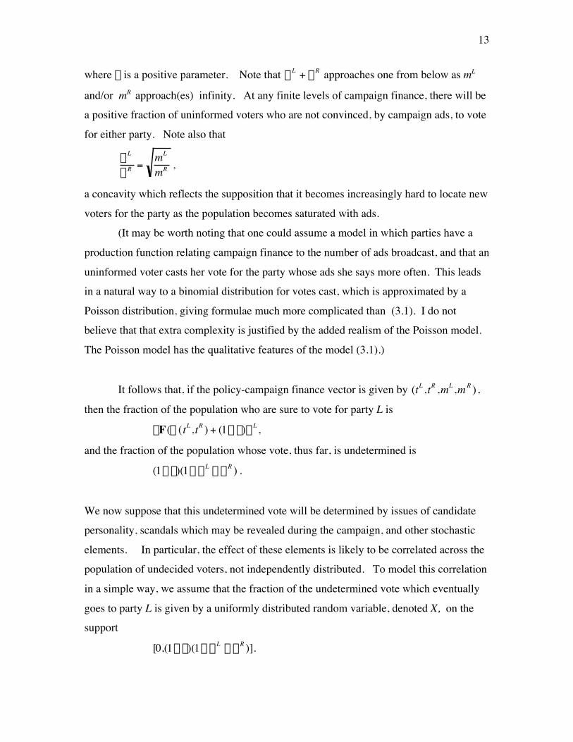
In addition to these six desiderata, we may add, finally, a methodological
desideratum:
7. Equilibria should be easy to compute, and locally unique, so that important
questions of comparative statics may be studied.
One must note that the financing of parties is not the only locus at which money
enters into politics, the other one being the lobbying process. Recently, Grossman and
Helpman (2001) have studied the role of money in politics. Much of their book is
concerned with modeling the lobbying process. They do, however, contribute, as well,
to the theory of campaign finance: in chapter 10, they study political equilibrium in
which campaign contributions of interest groups have an effect on the distribution of
votes between parties. It will be more fruitful to compare their theory with the present
one in the concluding section.
After having formulated the theory of political equilibrium with private campaign
finance, we can easily amend it to model three other financing institutions:
(1) privately financed parties with a legal cap on contributions;
(2) publicly financed parties, where each party receives a public subsidy in
proportion to its size (that is, each citizen brings an equal public subsidy to the party she
joins);
(3) publicly and privately financed parties, where each party receives public funds
matching its private contributions.
(The American system is complex, but is approximated by a combination of institutions
(1) and (3).)
7
We will make these amendments, and then compare the nature of the political
equilibria that would obtain under the various financing institutions. Our central concern
will be the degree to which these institutions produce results that conform to a common
conception of good representation.
In section 2, I introduce a new concept of equilibrium in environments with
cooperative ventures, which will later be a foundation of the concept of political
equilibrium. In section 3, I describe the environment of the politico-economy. Section
4 presents the equilibrium concept for an environment under our first institution,
unconstrained private campaign finance. Section 5 presents an interesting
characterization of the equilibrium, and shows how to compute it. Section 6 applies the
model to an example, computes equilibrium, and presents some comparative statics.
Section 7 presents the equilibrium concept for an environment with constrained private
campaign financing, where there is a legal cap on contributions, and computes the
equilibria for our canonical example, for various values of the cap on contributions.
Section 8 presents the definition of political equilibrium with public financing, for this
environment, and computes the equilibria for the canonical example of section 6, under
both public institutions described above. Section 9 concludes with a summary of the
comparisons among the financing institutions, and some brief welfare analysis.
2. Kantian equilibrium
In this section, I introduce a general notion of equilibrium in a public-good
setting. In later sections, it will be applied to the problem of campaign finance.
8
Consider an economy with N members. Each is endowed with a private good.
The economy produces a public good according to the technology
†
y = Q(x1,..., xN ) , where
xi is the contribution to the public good by individual i, in units of the private good, and y
is the level of the public good. The utility functions of the individuals are given by:
which we express in terms of a personalized cost of giving and a personalized utility from
the public good.
Denote by x the vector of contributions and by v the vector of utility functions.
We define:
Definition 1. A vector of contributions
†
(x1*,..., xN
* ) is a Kantian equilibrium for the
economy v if no individual would prefer that all individuals increase or decrease their
contributions by any given factor r >0.
Thus, at a Kantian equilibrium, there is unanimous agreement that, along the ray
of possible contributions defined by the contribution vector x*, the vector x* itself is the
best one.
In the differentiable case, if a contribution vector x* is Kantian , then the
functions of a real variable r defined by
†
ui(r) =
†
v i(rx1*, ...,rxN
* ) (2.1b)
are maximized, for all i= 1.,,,N, at r=1.
In a Nash equilibrium, each agent assumes that if she alters her behavior, the
behavior of all others remains fixed. In a Kantian equilibrium, she assumes that if she
alters her behavior, all others will alter theirs in like manner (in the sense of equi-
proportional changes). Our concept inherits its name from the Kantian imperative: Take
9
an action if and only if you would have all others do likewise. The idea was first
introduced in Roemer (1994, Chapter 6), although it was not formalized there in the
present manner.
A vector of contributions x is Pareto efficient if there is no vector of contributions
at which all individuals are at least as well off, with at least one individual better off.
We have the following result:
Proposition 1. Let the functions ci be convex and differentiable, and the functions hi and
Q be concave, differentiable, and strictly increasing. Let x* > 0 be a Kantian
equilibrium. Then x* is Pareto efficient.
We prove the proposition after establishing two lemmas.
Lemma 1. If there are positive numbers
†
{li} such that
†
li —v i(x) = 0 , (2.2)
then x is Pareto efficient.
(
†
—v i is the gradient vector of vi .)
Proof: By concavity of v’s, it suffices to show x is locally Pareto efficient. Suppose, to
the contrary, there were a direction
†
d ŒRN at x such that
†
"j ≠ i —v j(x) ⋅ d ≥ 0,
with at least one strict inequality. Then it follows from (2.2) that
†
—v i(x) ⋅ d < 0 ,
which shows that x is Pareto efficient.
Lemma 2. Let
†
a1,...,aN be positive numbers; let (
†
r1,...,rN ) be a positive vector in the
unit simplex SN. Then there exist positive numbers
†
l1,...,lN such that
10
†
"jl ja j
l iaiÂ= r j .
Proof:
Let
†
l j =r j
a j.
Proof of proposition 1:
Setting the derivative with respect to r of the functions
†
ui(r) =
†
v i(rx1*, ...,rxN
* ) equal to
zero at r=1, the condition for Kantian equilibrium gives:
†
"j h j¢(x j* )—Q(x*) ⋅ x* = c j ¢(x j
* )x j* (2.3)
Compute that for any distinct pair (i,j):
†
∂vi
∂xi (x*) = -ci¢ (xi*) + hi¢(Q) ∂Q
∂xi(x*),
∂vi
∂x j (x*) = hi¢ (Q) ∂Q∂x j
(x*).
It follows that (2.2) holds iff
†
"j l ihi
i ¢(Q) ∂Q
∂x j(x*) = l jc
j¢(xi* ). (2.4)
For each j, multiply both sides of equation (2.4) by
†
x j* and substitute from (2.3), yielding:
†
"j x j* ∂Q
∂x jli
i hi¢(Q) = l jh
j ¢(Q)(—Q ⋅ x*),
or:
†
"j,x j * ∂Q
∂x j
—Q(x*) ⋅ x * l i hi¢ (Q) = l jhj¢ (Q) . (2.5)
Now let
†
r j =
x j * ∂Q∂x j
—Q(x*) ⋅ x *, a j = h j ¢(Q). The premises of Lemma 2 hold, and it follows
that there exists a vector of positive l’s such that (2.5) holds. Hence, by Lemma 1, x* is
Pareto efficient. n
11
There is a link between Kantian equilibrium and Lindahl equilibrium. Silvestre
(1984) shows that, in the presence of convexity and differentiability assumptions (whichwe have in the premise of proposition 1), an allocation which is Pareto efficient and has
the property that no citizen would like all citizens to decrease their contributions to thepublic good by the same amount is a Lindahl equilibrium. Our definition of Kantian
equilibrium does not mention Pareto efficiency, but given proposition 1, a Kantian
equilibrium in a convex, differentiable environment satisfies the premises of Silvestre’sresult. It is therefore a Lindahl equilibrium.
The virtue of the Kantian conception, in contrast to the Lindahl conception, is thatthere are no personalized prices for the public good. The interesting fact is that
unanimous optimality along a ray (which is the definition of K-equilibrium) implies
efficiency.
3. The political environment and the probability-of-victory function
A. The environment
There is a sample space of citizen types H, with generic type h, distributedaccording to a probability measure denoted F on H. In the case that H is a real interval,
we denote the distribution function of F by F. There is a policy space T which we take
to be an interval on the real line. Voters are endowed with money , and the amount ofmoney they have will be an aspect of their type. A voter may make a contribution to a
political party. A voter of type h who contributes m in campaign contributions to parties
enjoys a utility of uh(t,m) if
†
t ŒT is the realized policy. We assume that
†
uh (⋅,⋅) is a von
Neumann-Morgenstern utility function for all h.
Political parties will eventually form and propose policies. We assume that,
within each type, a fraction of voters are ‘informed’ and the remainder are ‘uninformed.’
An informed voter can observe the policy announcements of parties, and compute herutility. An uninformed voter cannot observe policies: he observes only campaign
advertisements made by parties. We assume that uninformed voters tend to vote for theparty whose ads they see more often, an assumption that will be formalized presently.
12
The key here is that policies influence the votes only of informed voters, and advertising
influences the votes of only the uninformed.For simplicity, we assume throughout that the fraction of informed voters is the
same number r in all types.
In the applications that we study, the probability distribution F is assumed to becontinuous. There is a continuum of types, and no type has positive measure.
To avoid generality that would be gratuitous, we specialize to the quasi-linear
case, where utility is given by:
† †
uh (t,m) = v h (t) - m.
B. Electoral uncertainty
Suppose there are two parties, which will announce policies
†
t1,t2 ŒT . Define the
set of types whose members prefer t1 as:
†
W(t1,t2) = {h | vh (t1) > vh (t2 )} .
By the quasi-linear assumption, this set of types is invariant over the vectors of campaigncontributions that individuals have made. Facing a choice between t1 and t2, all informed
voters in
†
W(t1,t2) will vote for t1, and so party 1 would immediately win a fraction
†
rF(W(t1,t2 )) of votes.
We now assume that the fraction of the uninformed vote going to the two partiesdepends upon their campaign budgets. Let mJ be the campaign chest of party J,
measured in the dollars per capita that it can spend, which is assumed to be the
contributions per capita it has received, where ‘per capita’ means per population member,not per party member. Call, now, the parties L and R. We assume that, if the campaign
chests are
†
(m L ,mR ) then the fraction of the uninformed voters who vote for parties L and
R are given by:
†
jL =b m L
1+ b( mL + mR ),
jR =b m R
1 +b( m L + m R )
, (3.1)
13
where b is a positive parameter. Note that
†
jL + jR approaches one from below as mL
and/or mR approach(es) infinity. At any finite levels of campaign finance, there will bea positive fraction of uninformed voters who are not convinced, by campaign ads, to vote
for either party. Note also that
†
jL
jR =mL
mR ,
a concavity which reflects the supposition that it becomes increasingly hard to locate new
voters for the party as the population becomes saturated with ads.(It may be worth noting that one could assume a model in which parties have a
production function relating campaign finance to the number of ads broadcast, and that an
uninformed voter casts her vote for the party whose ads she says more often. This leadsin a natural way to a binomial distribution for votes cast, which is approximated by a
Poisson distribution, giving formulae much more complicated than (3.1). I do notbelieve that that extra complexity is justified by the added realism of the Poisson model.
The Poisson model has the qualitative features of the model (3.1).)
It follows that, if the policy-campaign finance vector is given by
†
(tL ,tR ,mL ,m R ) ,
then the fraction of the population who are sure to vote for party L is
†
rF(W(tL ,tR ) + (1- r)jL ,
and the fraction of the population whose vote, thus far, is undetermined is
†
(1- r)(1- jL - jR ) .
We now suppose that this undetermined vote will be determined by issues of candidatepersonality, scandals which may be revealed during the campaign, and other stochastic
elements. In particular, the effect of these elements is likely to be correlated across thepopulation of undecided voters, not independently distributed. To model this correlation
in a simple way, we assume that the fraction of the undetermined vote which eventually
goes to party L is given by a uniformly distributed random variable, denoted X, on thesupport
†
[0,(1- r)(1- jL - jR )].
14
Consequently, the fraction of the population who votes for L is
†
rF(W(tL ,tR ) + (1- r)jL + X ,
and it follows that the probability that L wins the election is given by:
†
p(tL ,tR,m L ,mR ) = prob[rF(W(tL ,tR ) + (1- r)jL + X >12]
= prob[X >12 - rF(W(tL ,tR ) - (1- r)jL ]
= I[1 +rF(W(tL ,tR )) + (1- r)jL -
12
(1- r)(1- jL - jR ) ],
(3.2a)
where I is the ‘truncated identity function,’ defined by:
†
I(x) =
0, if x £ 0x, if 0 < x < 1
1, if x ≥1.
Ï
Ì Ô
Ó Ô
(The last line in expression (3.2a) is computed using the knowledge that X is uniformly
distributed on its support.)
We have thus defined the probability- of- victory function.
By substituting in for the expressions
†
jJ in (3.2) and simplifying, we have:
†
p(tL ,tR,m L ,mR ) = I[1 +b m L +(rF(W(tL ,tR )) -
12
)(1 +b( m L + m R ))
1- r] , (3.2b)
a nice, simple concave function of the campaign budgets.
The assumption that some voters are influenced only by policy and some voters
only by campaign ads is clearly extreme; it is a stylized assumption that leads to fairly
simple formulae in the analysis below.
4. Political equilibrium with private finance
15
A. Determination of policy
We propose how policy is determined, if the membership of parties is given and
the contributions of members to their parties are given. Thus, let
†
H = L » R, L « R = ∅ ,
be a partition of the space of types, where the informed voters of type h
†
ΠL form party L
and the informed voters of type h
†
ΠR form party R. We assume that there is perfect
coordination among informed citizens of the same type, so that every informed citizen of
given type makes exactly the same campaign contribution. Let
†
{m h | h ŒL} and {m h | h ŒR} be the campaign contributions of the parties’ members to
their parties. Thus the(population) per capita contributions are given by:
†
mL = r m h
hŒLÚ dF(h), m R = r m h
hŒRÚ dF(h) .
Each informed citizen is interested in his party’s proposing a policy that maximizes his
expected utility, given the policy that the opposition party is proposing. For instance,
given that party R proposes policy tR, a member of type h of party L would like her party
to propose the policy t that maximizes
†
p(t,tR,m L ,mR )v h (t) + (1- p( t,tR,m L ,mR ))vh (tR ) - m h . (3.3)
We now assume that the members of each party bargain with each other over policy,
where the bargaining power of a particular type is proportional to its contributions to the
party. In this bargaining game, the threat point for members of party L is the utility
realized if their party fails to agree on a policy, and hence the opposition party wins the
election by default, in which case all members of party L sustain the utility
16
†
v h(tR ) - m h . (3.4)
The utility gain of member h of L at a policy bargain tL reached in L from the threat
point, is hence the difference between the expressions (3.3) and (3.4), which we write as:
†
p(tL ,tR,m L ,mR )Dvh (tL ,tR ) , (3.5a)
where Dv is the difference operator:
†
Dv(x, y) = v(x) - v(y).
In like manner, the utility gain to member h of party R from her threat point, when facing
a policy tL from the opposition, is:
†
(1- p)Dv h (tR,tL ) . (3.5b)
Expressions (3.5 a and b) have the natural interpretation that the utility gain is the product
of the probability of one’s party’s victory and the utility difference enjoyed from one’s
party’s victory.
We now model the intra-party bargaining process by taking a cue from the Nash
bargaining game: that is, we assume that the policy bargain reached maximizes the
product of the bargainers utility gains from their threat points, raised to the powers of
their bargaining powers. Expressing this in logarithmic form, we have that:
†
tL = argmaxtŒT
mh
LÚ log[p( t,tR ,mL ,m R )Dvh (t,tR )]dF(h),
tR = argmaxt ŒT
m h
RÚ log[(1- p(tL ,t,mL ,m R ))Dv h (tL ,t)]dF(h). (3.6)
To summarize, we say that:
Definition 3. A policy pair
†
(tL ,tR ) is a policy equilibrium for the parties L and R in a
partition
†
H = L » R at contribution levels
†
{m h | h ŒL} and {m h | h ŒR)} if equations
(3.6) hold.
17
It goes almost without saying that each member of a party prefers its party’s
policy to the opposition’s policy, because, were that false, then the logarithms in (3.6)
would be undefined. So if a policy equilibrium exists, we are guaranteed that every
party member prefers his party’s policy to the opposition’s.
We note that the present theory is incapable of explaining what sometimes occurs
in reality, that some citizens contribute money to more than one party; see Steen and
Shapiro (2002) for discussion. It would seem that the phenomenon of ‘walking both
sides of the street’ is explained by the desire of contributors to have ‘access’ to office
holders after the election; in contrast, in our environment, all issues are decided prior to
the election. Access after the election would be important if the platform is an
‘incomplete contract,’ so to speak, and so many issues will be settled as they come up
over time, after the election. In the complete contract setting of the present theory, access
to the winner after the election would be of no value.
B. Determination of campaign contributions
We next propose how campaign contributions are determined, at a given pair of
policies
†
(tL ,tR ). Here, we invoke the notion of Kantian equilibrium. Denote an (infinite
vector) of campaign contributions to party L by ML, with the analogous meaning for MR.
At a particular vector of policies, and given the campaign contributions of the opposite
party, we can write the expected utility of an informed voter of type h of party L as a
function of the (infinite) vector of campaign contributions made by his party’s members
as:
18
†
U h (ML ,m h;m R ) = p( tL ,tR,mL ,m R )vh (tL) + (1- p)vh (tR ) - m h, (3.7a)
where mL is derived from ML according to the formulae provided at the beginning of part
A of this section. The analogous representation for the utilities of party R’s members is
given by the same formula, that is:
†
U h (MR ,mh ;mL ) = p( tL ,tR,mL ,m R )vh (tL) + (1- p)vh (tR ) - m h, (3.7b)
We are now in the environment of a Kantian equilibrium, where the relevant utility
functions of the party members are the functions Uh. Clearly, if every party member
were to increase (decrease) his contribution by a factor r, then the budget of the party
would increase (decrease) by the same factor.
Definition 4. Vectors of contributions ML and MR to two parties at a given policy vector
†
(tL ,tR ) comprise a contribution equilibrium at
†
(tL ,tR ) if ML is a Kantian equilibrium for
the members of L , with respect to the utility functions
†
{U h | h ŒL} , given MR, and MR is
a Kantian equilibrium for the members of party R with respect to the utility functions
†
{U h | h ŒR} , given ML.
In other words, it is assumed that parties co-ordinate members’ contributions in
order to realize a Kantian equilibrium in contributions. Note that, in the thought
experiment that Kantian equilibrium proposes, all members’ contributions would increase
by the same factor, and hence the relative bargaining powers of the members would not
change.
We cannot immediately apply Proposition 1 to this environment, because in the
proposition, the environment assumed a finite number of types, and here we are working
with a continuum. Nevertheless, if we here assume a finite number of types, so that
19
†
mL = f h
hŒLÂ mh , then we can immediately observe , from equation (3.2b), that the
functions Uh are concave in the contributors’ contributions, and hence a Kantian
equilibrium in contributions is Pareto efficient from the contributors’ viewpoints.
Let us review the motivation for invoking Kantian equilibrium here. We wish to
model the idea that parties are associations of citizens that provide public goods to their
members – two, in fact -- their policy and their campaign ads, financed by the campaign
chest. We model policy as being produced by competition among members. We model
the campaign chest as produced by coordination among members and competition
between parties. How could a party coordinate member contributions? We have
proposed a very simple rule: it can appeal to all members to increase (or decrease!) their
contributions by a given proportion. This rule, as well as being extremely simple, has
the virtue of not interfering with the process by which policy is arrived at, because a call
to change proportionally all contributions will not alter the nature of the bargaining
problem among party members over policy. And finally we have shown that this rule
successfully coordinates individual behavior, in the sense that, when no such
proportionate changes are justified, the provision of the public good of campaign finance
is Pareto efficient for the set of party members.
C. Political equilibrium with contributions
We now define a full political equilibrium by combining the previous two
concepts.
Definition 5 A political equilibrium with unconstrained contributions consists of:
(1) a partition
†
H = L » R, L « R = ∅ ,
20
(2) vectors of contributions
†
M L = {m h | h ŒL}, MR = {mh | h ŒR} from the
informed members of types to their parties,
(3) policies tL and tR of the two parties,
such that:
(4) (tL, tR) is a policy equilibrium at contribution vectors ML, MR, and
(5) ML and MR comprise a contribution equilibrium at (tL, tR).
We should note that the equilibrium concept fulfills the six desiderata listed in the
introduction. Each policy is a best response to the other party’s policy, where the ‘utility
function’ of a party is that function which is optimized at the solution of a Nash
bargaining game among the party’s members, a game in which the power of individual
types is proportional to their campaign contributions to the party. Campaign
contributions play a double role: they determine the strengths of citizen types in intra-
party bargaining, and they also determine the party’s ability to reach uninformed voters.
Moreover, with respect to this second purpose, the contributions are optimal as far as the
the members are concerned, because they are a Kantian equilibrium in that regard, given
the other components of the equilibrium. Finally, party membership is stable in the sense
that every type prefers its party’s policy to the opposition’s, and by the continuum
assumption, all types have negligible influence on donations and policy.
Two remarks are in order.
Remark 1. Party members do not determine their contributions with an eye to
optimizing with respect to their bargaining power in the intra-party bargaining game.
Now in the continuum model, individual types have no incentive to alter their
contributions, because, in an atomless economy, no type can alter the objective functions
21
in (3.6) by altering its contributions. In a finite- type economy, we would have to
consider this kind of strategic behavior, and then the political equilibrium would be over-
determined: in most cases, no equilibrium would exist.
In the continuum model, as we shall see, equilibria do exist and are well-defined,
that is, locally unique.
Remark 2. The party is an association which organizes the campaign-contribution
behavior of its members in a cooperative fashion; we must say that there is space for this
kind of cooperation precisely because, with the continuum assumption, no type can have
any strategic gain by altering its contribution. We have modeled that cooperative
function of the party with the Kantian equilibrium concept, which has normative appeal
as a cooperative solution concept. One may object that it is not clear how the party
would implement this cooperative solution – how it would find the Kantian equilibrium
in contributions; a similar statement is often made with respect to Lindahl equilibrium in
a public-goods economy, and we have noted that Kantian equilibrium is a special case of
Lindahl equilibrium.
In defense of our concept, however, it must be noted that even Walrasian
equilibrium is only a normative concept, despite frequent claims to the contrary, because
we have no robust theory of how ‘the market’ finds the Walrasian equilibrium5. If the
market somehow finds a Walrasian equilibrium, then there is reason for it to be stable
(because all markets clear under optimizing behavior of traders). Similarly, if parties
find the Kantian equilibrium in contributions, then contributions are stable, in the sense
5 In other words, a purely positive concept of market equilibrium, I am proposing, would describe how the
equilibrium is arrived at, as well.
22
of unanimous agreement of members about proposals to change proportionally all
contributions.
Indeed, we must say that the present model is only plausible given the assumption
of an atomless set of citizen types. This equilibrium is not the limit of a similar sequence
of equilibria in finite type economies, as the number of types increases, because in those
economies, we would have to allow members to optimize individually on their campaign
contributions6.
5. A characterization of private political equilibrium and the computation of equilibrium
A. General computation of equilibrium
We first compute the first-order conditions for a Kantian equilibrium in
contributions. This involves using the expression (3.7a) and setting the derivative of
†
U h (rM h,rmh ;mR ) , with respect to r, equal to zero at r=1. The F.O.C.s are:
for all h in L,
†
mh =∂p
∂mL m LDv h (tL ,tR )
for all h in R,
†
mh =∂(1- p)
∂mL mR Dv h (tR,tL ) .
These two equations can be conveniently expressed together as:
†
(for J = L,R)("h ŒJ)(mh =∂p
∂mJ mJ Dv h (tL ,tR )), (5.1)
6 It should here be noted that Walsrasian equilibrium is not logically plausible for a finite economy either,
because in such economies, individuals have the power to influence prices, and it is therefore inconsistent
that they should treat prices as given, as they do in Walrasian equilibrium. Truly competitive equilibrium
usually fails to exist in finite economies, as well! For discussion, consult Makowski and Ostroy (2001).
23
where it is understood that the function p is evaluated at
†
(tL ,tR ,mL ,m R ). Using the fact
that
†
mJ = r m h
hŒJÚ dF(h) , we can integrate equations (5.1) dF(h) and divide by mJ,
yielding:
for J=L,R :
†
1r
=∂p
∂mJ Dvh
JÚ (tL ,tR)dF(h). (5.2a,b)
We next compute the first-order conditions for (tL, tR) to be a policy equilibrium.
From (3.6), we may write:
†
tL = argmaxt
[ mL
rlog p(t, tR,m L ,mR ) + mh
hŒLÚ log Dv h (t,tR )dF(h)],
tR = argmaxt
[m R
rlog(1- p(tL ,t,mL ,m R )) + mh
hŒRÚ log Dv h (t,tL )dF(h)] .
Differentiating these expressions w.r.t. t, and setting the derivatives equal to zero
produces:
†
mL
p
∂p
∂tL + rm h
Dvh (tL,tR )LÚ
∂v h
∂t(tL )dF(h) = 0 (5.3a)
-m R
1- p∂p∂tR + r
m h
Dvh (tR ,tL)RÚ
∂v h
∂t (tR )dF(h) = 0 (5.3b).
We now use the continuum of equations (5.1) to substitute for mh in expressions
(5.3a,b), which simplifies the latter to:
†
1p
∂p
∂tL + r∂p
∂m L
∂vh
∂tLÚ (tL)dF(h) = 0 (5.4a)
11- p
∂p∂tR + r
∂p∂mR
∂vh
∂tRÚ (tR )dF(h) = 0 (5.4b)
.
(yes, the signs are correct!)
24
Now notice that equations (5.2a,b) and (5.4a,b) comprise four equations in the
four unknowns
†
(tL ,tR ,mL ,m R ) . How do we determine the (L,R) partition? We simply
note that
†
L = {h | vh (tL) > v h (tR )}R = {h | v h (tR ) > v h (tL )}
. (5.5a,b)
Therefore, (5.2 a,b), (5.4a,b) and (5.5 a,b) comprise six equations in six unknowns (the
last two being L and R) which, hopefully, will possess a solution. If we can solve them,
then the contributions of individual types are immediately computed from (5.1).
B. An interesting characterization of equilibrium
Using equations (5.2a,b), solve for
†
dpdmL and dp
dm R , and substitute these
expressions into equations (5.4a,b), which produces, after some minor re-writing:
†
1p
∂p
∂tL + [ Dv h
LÚ (tL ,tR )dF(h)]-1 dvh
dtLÚ (tL)dF(h) = 0 (5.6a)
-11- p
∂p∂tR + [ Dvh
RÚ (tR,tL)dF(h)]-1 dv h
dtRÚ (tR )dF(h) = 0 (5.6b)
Now define the functions:
†
V L(t) ≡ vh
LÚ (t)dF(h), V R (t) ≡ v h
RÚ (t)dF(h) .
Then (5.6a,b) can be written, after some minor algebraic manipulation:
†
∂p
∂tL (V L (tL ) -V L(tR)) + pdV L
dt(tL ) = 0 (5.7a)
∂(1- p)∂tR (V R (tR ) -V R (tL)) + (1- p) dV R
dt (tR ) = 0 (5.7b)
But these equations are equivalent to the following first-order conditions:
25
†
ddt
[pV L(t) + (1- p)V L (tR )] = 0 at t = tL (5.8a)
ddt [pV R (tL ) + (1- p)V R (t)] = 0 at t = tR (5.8b)
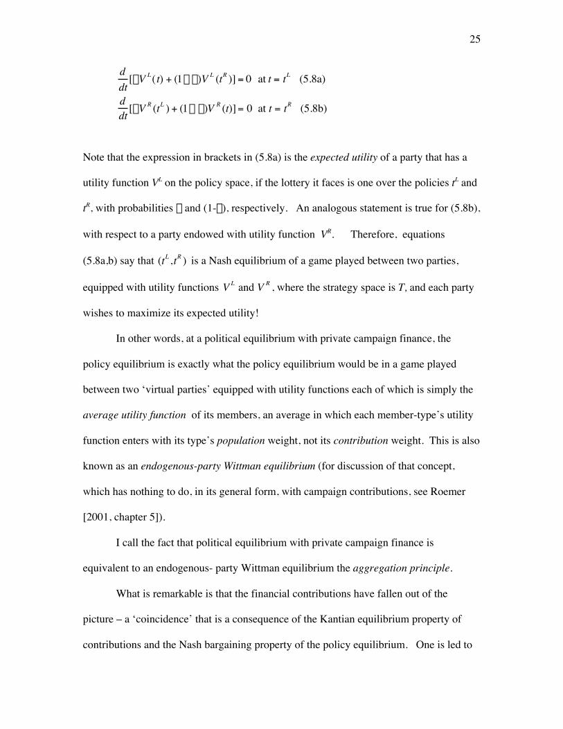
Note that the expression in brackets in (5.8a) is the expected utility of a party that has a
utility function VL on the policy space, if the lottery it faces is one over the policies tL and
tR, with probabilities p and (1-p), respectively. An analogous statement is true for (5.8b),
with respect to a party endowed with utility function VR. Therefore, equations
(5.8a,b) say that
†
(tL ,tR ) is a Nash equilibrium of a game played between two parties,
equipped with utility functions
†
V L and V R , where the strategy space is T, and each party
wishes to maximize its expected utility!
In other words, at a political equilibrium with private campaign finance, the
policy equilibrium is exactly what the policy equilibrium would be in a game played
between two ‘virtual parties’ equipped with utility functions each of which is simply the
average utility function of its members, an average in which each member-type’s utility
function enters with its type’s population weight, not its contribution weight. This is also
known as an endogenous-party Wittman equilibrium (for discussion of that concept,
which has nothing to do, in its general form, with campaign contributions, see Roemer
[2001, chapter 5]).
I call the fact that political equilibrium with private campaign finance is
equivalent to an endogenous- party Wittman equilibrium the aggregation principle.
What is remarkable is that the financial contributions have fallen out of the
picture – a ‘coincidence’ that is a consequence of the Kantian equilibrium property of
contributions and the Nash bargaining property of the policy equilibrium. One is led to
26
ask: where, then, is the ‘distortion’ in policies due to the fact that types are represented in
parties according to their contributions, rather than according to their numbers? The
answer is that that distortion is reflected in the probability function. In equations
(5.8a,b), the derivatives are with respect to policies only, but the campaign contributions
enter, of course, into the probability functions, and therefore the values of those functions
are (very) different from what they would be, were every member to contribute the same
amount to her party.
From our knowledge of the behavior of endogenous-party Wittman equilibrium,
we can make a prediction about the nature of political equilibrium with private campaign
finance, in a polity where the policy concerns redistribution, and a citizen’s type is his
income or wealth. We know the equilibrium must be characterized by equations (5.8a,b)
and (5.2a,b) which can be written, now, as:
†
1r
=∂p
∂mL m LDV L(tL ,tR)
1r
=∂(1- p)
∂m R mR DV R (tR,tL ).
In such an environment, we can expect that the parties will endogenously form to
represent the upper and lower parts of the wealth distribution, with some cut point. The
fact that the rich will contribute more, loosely speaking, to their party than the poor will
have the consequence that the party representing the upper part of the distribution will be
small and the other party will be large. This will be the consequence of the distortion of
the probability function entailed by disproportional contributions of the rich and the poor.
Thus, we predict that we will observe a political equilibrium with a small party
representing the very rich, and a large party representing all others.
27
Before proceeding with the analysis of an example to check whether this
prediction is borne out, a warning to the reader is in order. We have assumed two things
about utility functions: first, that they are von Neumann- Morgenstern, and second, that
they are quasi-linear in contributions. No interpersonal comparability of utility has been
assumed. What does this mean about the average functions VJ, J=L,R ? It means that we
cannot interpret VL(t) as a meaningful average welfare level of the members of party L.
For to do so, the individual utility functions would have to be cardinally unit comparable
– that is, the utility they measure would have to in units that are interpersonally
comparable in a meaningful way7. Consider again an example where a person’s type is
is her wealth. With the quasi-linear family of utility functions we have chosen, the
marginal disutility of contributing $1 is the same for all citizens. Clearly, in
interpersonally comparable units, this statement is false in actuality: we believe it is much
less costly for a rich person to contribute a dollar than a poor person. Therefore, the right
family of utility functions for purposes of interpersonal comparability is not the quasi-
linear family. Another way of saying this is that it would be an error to interpret VL and
VR as utilitarian functions – because the aggregation of individual utilities they perform is
not interpersonally meaningful.
Thus, the aggregation principle is a formal property of political equilibrium. It
must not be thought to imply that the virtual parties of equations (5.8a,b) are maximizing
the average expected welfare of their members8.
7 The measurement and comparability of utility is a topic of social choice theory. For a discussion, the
reader is referred to Roemer[1996, Chapter 1].8 Social choice theorists will recognize that this point occurs as well in the debate over Harsanyi’s theorems
on utilitarianism. For a discussion, the interested reader is again referred to Roemer[1996, Chapter 4].
28
6. An example
We now specialize to the case, for computational purposes, where T=H=R+, and
assume Euclidean preferences:
†
v h(t) = -a h
2 (t - h)2 .
Think of h as income or wealth and th=h, as the ideal policy for type h. Since utility is
quasi-linear in contributions, the constants ah will allow us to model the idea that the
trade-off between policy and contributions is different for types of different wealth.
Given two policies (tL,tR), the indifferent type is
†
h *(tL ,tR ) =tL + tR
2 , and the
associated partition of types into parties is
†
L = {h < h*}, R = {h > h*}. (Here, we have
identified party L with the ‘poor’ types; hence the nomenclature Left and Right.) If
†
tL < tR, then
†
W(tL ,tR ) = {h < h*} , and it follows that
†
F(W(tL ,tR )) = F(h*) , where, recall,
F is the C.D.F. of F.
Denote
†
t = tL + tR
2 . Then
†
Dvh (tL ,tR ) = ah Dt(-t + h), where
†
Dt = tL - tR . Now
define:
†
a 0L =
a h
0
h*
Ú dF(h)
F (h*), a 0
R =
ah
h*
•
Ú dF(h)
1- F(h*),
a1h =
ha h
0
h*
Ú dF(h)
F(h*), a1
R =
hah
h*
•
Ú dF(h)
1- F (h*).
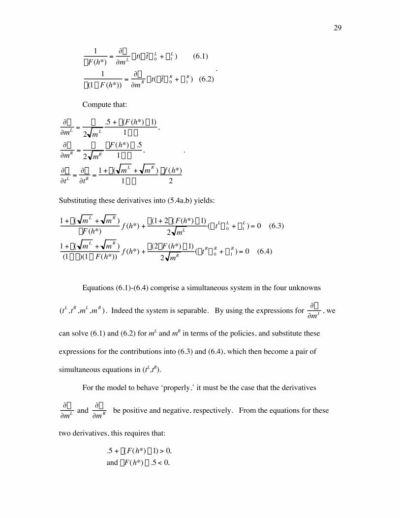
Then we may write (5.2a,b) as:
29
†
1rF(h*)
=∂p
∂m L Dt(- t a 0L + a1
L ) (6.1)
1r(1- F (h*))
=∂p
∂m R Dt(-t a 0R + a1
R ) (6.2).
Compute that:
†
∂p∂mL =
b
2 m L
.5 + r(F (h*) -1)1- r
,
∂p∂mR =
b
2 mR
rF(h*) - .51- r
,
∂p∂tL =
∂p∂tR =
1 +b( m L + m R )1- r
rf (h*)2
.
Substituting these derivatives into (5.4a,b) yields:
†
1 +b( m L + m R )pF (h*) f (h*) +
b(1+ 2r(F(h*) -1)2 mL
(- tLa 0L + a1
L ) = 0 (6.3)
1 +b( m L + m R )(1- p)(1- F(h*)) f (h*) +
b(2rF (h*) -1)2 mR
(-tRa 0R + a1
R ) = 0 (6.4)
Equations (6.1)-(6.4) comprise a simultaneous system in the four unknowns
†
(tL ,tR ,mL ,m R ) . Indeed the system is separable. By using the expressions for
†
∂p∂mJ , we
can solve (6.1) and (6.2) for mL and mR in terms of the policies, and substitute these
expressions for the contributions into (6.3) and (6.4), which then become a pair of
simultaneous equations in (tL,tR).
For the model to behave ‘properly,’ it must be the case that the derivatives
†
∂p∂mL and ∂p
∂m R be positive and negative, respectively. From the equations for these
two derivatives, this requires that:
†
.5 + r(F(h*) -1) > 0,and rF(h*) - .5 < 0,
30
which reduce to :
†
r < min[ .51- F (h*), 1
2F (h*)]. (6.5)
We now present a specific example, parameterizing the model as follows:
†
b = 0.1, ah =hd
100 , F is the lognormal distribution with mean 40 and median 30. We
choose, initially, d = 1. We think of type h as the type with annual income of h
thousands of dollars; then the F looks like the US income distribution in the early 1990s.
Note that the marginal rate of substitution between contributions and policy
†
( dtdm ) for
type h is
†
a h(t - h) , so making ah an increasing function of h means that this MRS is
larger, for a small change in policy near a type’s ideal point, for the rich than for the poor
– thus, we would expect the rich to contribute more to campaigns than the poor. The
larger is the exponent d, the faster will the MRS of policy against campaign contributions
increase with h.
In table 1, I report the values of political equilibria for various values of r, at
d=19. The first five columns are self-explanatory. Columns 6 and 7 give the centile of
the type, in the income distribution, whose ideal policy is the Left policy and the Right
policy, respectively. Column 8 gives the centile in the income distribution of the type
which defines the cut-point between membership in the two parties. In other words, the
fraction of the polity represented by the Left party is exactly the value in column 8.
Column 9 gives the probability of victory of Left. Column ‘exp pol” is the centile of the
9 All computations were programmed in Mathematica; the programs are available from the author, uponrequest.
31
type whose ideal policy is the expected policy,
†
ptL + (1- p)tR . And the last column,
‘com’, reports the fraction of voters who finally, after advertising, are committed to one
of the parties, that is,
†
1- (1- r)(1- jL - jR ) . (In other words, the votes of the fraction
‘1-com’ of the population are governed by the random variable X.)
[table 1 here]
Perhaps the two must important statistics are those in the F[tbar] and ‘exp pol’
columns. We see that, for small values of r, our prediction is true: equilibrium entails a
small party of the Right, representing the top 20 percent of the wealth distribution, and a
large party representing all others. The expected policy is quite right-wing: for example,
at r=0.4, it is the ideal policy of the type at the 70th centile of the wealth distribution. At
r=0.4, the Left (Right) party proposes the ideal policy of the type at the 61st centile (89th
centile) of the income distribution. We see that, in this equilibrium , Left spends a little
more than Right in the election – but it spends only about one-fourth the amount per
party member, since there are four times as many members in Left as in Right. Thus, the
large individual expenditures of Right members on the campaign enable a minority Right
party to survive – in the sense of having a positive probability of victory.
As the population becomes more informed (r increases), politics become less
skewed, so that at r=.775, the Left represents 55% of the population, and the Right 45%.
The expected policy is a little to right of the ideal policy of the median wealth holder.
Campaign spending decreases quite radically as the population becomes more informed:
this occurs because there are fewer voters to be convinced by campaign ads. Note also
that for large values of r, the Right spends much more than Left: at r=.775, Right is
32
spending 47 times as much as Left. We cannot attach any dollar meaning to the per
capita campaign chests of the two parties, as we do not know the units of money. The
ratio of the campaign contributions is, however, relevant.
We can understand the sense in which politics become right-wing when r is small
by invoking the aggregation principle. When r=0.4, the Right party represents the
richest 20% of the income distribution. The Left party also has a significant number of
fairly rich people in it, because it represents the bottom 80% of the income distribution.
We can thus conjecture that it will propose policies that are not too far left. So both
parties will propose quite ‘conservative’ policies.
In other words, in a population whose party partition has a high cut point h* ,
politics will be fairly right-wing, and in a partition with a low cut point, politics will be
fairly left-wing, by analogous reasoning. We note that the equilibrium partition is always
to the right of the median income type in the equilibria of Table 1.
Why is a Right party that is so small at r= 0.4 politically feasible? Because the
Right is spending much more per member than is Left and so the probability of Right
victory is not as small as it ‘should’ be, given the policy of the Right. If all voters were
informed, 80% of the polity would vote for the Left policy, and the Right would lose the
election for sure. But if all voters were informed, this would not be the equilibrium
partition.
33
Figure 1: Contributions by type at the equilibrium of the example for r=0.4
In Figure 1, I plot campaign contributions as a function of h. Of course, it
follows from (5.1) that the indifferent type (the pivot) contributes zero. Contributions
approach infinity, as h approaches infinity.
Finally, we note that inequality (6.5) holds for all these equilibria, so we are in the
region where the model is well-behaved.
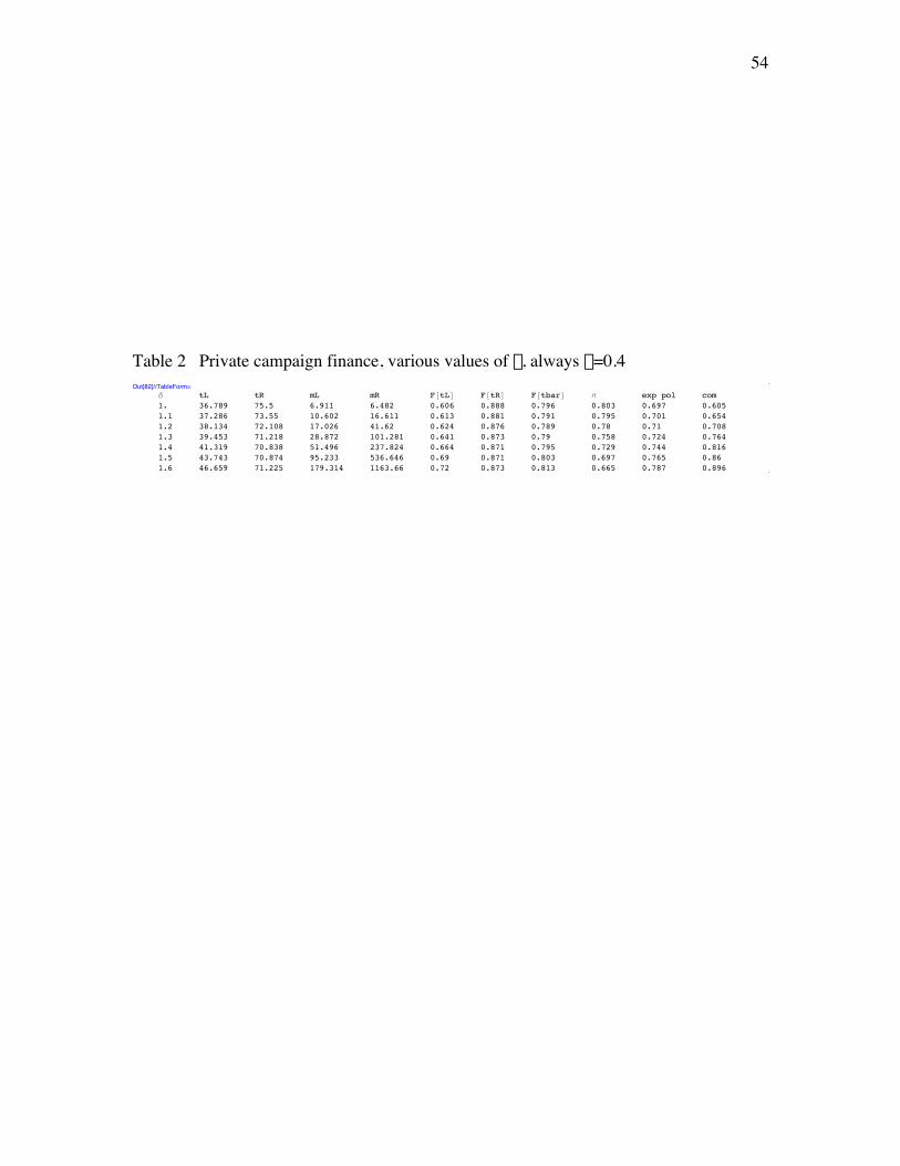
The next experiment is to observe what happens as we increase the value of the
exponent d. I fix r=0.4, and increase d from 1 to 1.6: the results are reported in Table 2.
[table 2 here]
As d becomes larger, citizens will want to spend more on campaigns, and the effect will
be magnified as h increases. We should therefore expect that the political equilibrium
will be even more skewed to the right, as d increases. We observe that this is indeed so
from Table 2: consult the ‘exp pol’ column. Curiously, the size of the Right party is not
monotonic in d, although it is always close to 20% of the polity. The most dramatic
observations from Table 2 are the extreme increase in Right spending as d increases, the
20 40 60 80 100h
10
20
30
40
50
60
contribution
34
movement of Left’s equilibrium policy to the right, and the decreasing probability of Left
victory.
7. Constrained private campaign finance
Our second financing institution is private finance with a cap on contributions.
To define political equilibrium for this institution, we must first generalize the definition
of Kantian equilibrium to this environment.
Consider the environment of section 2, and the utility functions vi of equation
(2.1). We now restrict the contributions xi to be bounded above by some number M0.
There are various conceivable generalizations of the notion of Kantian equilibrium to this
environment: our motivation for the choice below will soon be apparent.
Definition 6 Let x=
†
(x1, x2,..., xN ) be a vector of contributions for the ‘constrained’
environment with a contribution cap of M0 . Define the set
†
C = {i | xi = M0}. We say:
(1) If
†
C = ∅ , then x is a Kantian equilibrium just in case it satisfies definition 1;
(2) If
†
C ≠ ∅ , then x is a constrained Kantian equilibrium iff:
(a) no unconstrained agent
†
j œC would like to increase or decrease the
contributions of all agents by any factor r;
(b) no constrained agent
†
j ŒC would like to decrease the contributions of all
agents by any factor r.
It is important to understand that, in part 2(a) of the definition, r can be greater
than one. Thus, the condition allows unconstrained agents to contemplate infeasible
vectors of contributions.
35
Given the concavity and differentiability of the functions vi , we can characterize a
Kantian equilibrium by the first-order conditions:
†
"j œC ddr
v j(rx1,...,rxN ) = 0 at r =1
"j ŒC x j = M0 and ddr
v j (rx1, ...,rxN ) ≥ 0 at r = 1.(7.1)
In words, we can say that a constrained Kantian equilibrium is an allocation of
contributions such the contributors who are not constrained are unanimously pleased with
the vector of contributions (in the sense of 2(a)), while the constrained agents would like
everyone to increase his contribution, an action that is infeasible.
I claim this is the right generalization of Kantian equilibrium to the constrained
environment for two reasons: first, it will engender a locally unique equilibrium
allocation. This is easily seen. In case (1) we are back in the world of section 2. In case
(2), note that there will be
†
N- | C | first – order conditions from part 2(a), and |C|
equations of the form xj=M0 -- thus N equations in N unknowns. Second, Kantian
allocations, so defined, are again Pareto efficient, a fact which we now demonstrate.
Proposition 2 Let
†
x* = (x1*,..., xN
* ), x* > 0, be a Kantian equilibrium in the constrained
environment. Then x* is Pareto efficient.
To prove the proposition, we use the following lemma:
Lemma 3. Let the utility functions { vi} be concave. Let x be a vector of constrained
contributions, with
†
C = {i | xi = M0}. If there exist positive numbers
†
{li | i =1,.., .N} and
non-negative numbers
†
{ai | i ŒC} such that:
†
li
i —v i = a i
iŒCÂ ei , (7.2)
36
where ei is the ith unit vector in RN , then x is Pareto efficient.
Proof of Lemma:
By concavity, we need only show that x is locally Pareto efficient. Let
†
d ŒRN be a
feasible direction at x: then
for all
†
i ŒC, d ⋅ei £ 0 , (7.3)
because
†
xi = M0 for i ŒC . Suppose moving in direction d produces a Pareto
improvement: this means that
†
—v i(x) ⋅ d ≥ 0 for all i, with strict inequality for some i.
But taking the scalar product of equation (7.2) with d produces:
†
li
i —v i(x) ⋅ d £ 0 ,
by invoking (7.3), and so, since all the l’s are positive, we must have
†
—v i(x) ⋅ d = 0 for all i ,
a contradiction which proves the lemma. n
Proof of Proposition 2:
1. Let
†
C = {i | xi* = M0} . Denote the complement of C by
The analysis proceeds just as in section 2; a Kantian equilibrium is still Pareto efficient.
When we apply this to our political model, we define a political equilibrium with
matching public funds just as in Definition 5. I am therefore brief:
Definition 8 A political equilibrium with matching public funds is a partition
†
H = L » R, a pair of policies
†
(tL ,tR ) , a schedule of private contributions to parties
†
M L = {m h | h ŒL}, M R = {m h | h ŒR} , per capita private contributions to parties mL and
mR , and total party campaign chests zL and zR such that:
(1)
†
mJ = r m h
hŒJÚ dF(h), J = L,R
zJ = 2m J, J = L,R
(2) (ML,MR) is a contribution equilibrium, given
†
(L,R) and (tL ,tR )
(3)
†
(tL ,tR ) is a policy equilibrium, given
†
(L,R) and (zL ,z R ) .
45
The reader can now deduce that the equations for this equilibrium are almost like
(5.2a,b) and (5.4 a,b):
†
1r
= 2 ∂p
∂zL Dv h
LÚ (tL ,tR )dF(h) (8.6a)
1r
= 2 ∂p∂zR Dvh
RÚ (tL ,tR)dF(h) (8.6b)
1p
∂p
∂tL + r∂p
∂z Ldv h
dtLÚ (tL )dF(h) = 0 (8.6c)
11- p
∂p
∂tR + r∂p
∂zR
dv h
dtRÚ (tR )dF(h) = 0 (8.6d)
The numeral ‘2’ appears in (8.6a,b) because the F.O.C.s for Kantian equilibrium, with
this institution, are:
†
mh = 2 ∂p∂zL Dv h
LÚ (tL ,tR )dF(h) ,
(I illustrate for the Left), which integrates to (8.6a).
We compute the equilibria for the same set of environments as that described in
Table 1. The statistics are presented in Table 5. The interesting comparison is with
Table 1, the case of unconstrained private contributions. We see that , for every value of
r, politics move to the right with public matching, in the sense that the expected policies
are uniformly more favorable to the wealthy in Table 5 than in Table 1. The proximate
cause of this result can be gleaned from looking at the equilibrium private contributions.
For instance, in Table 1, at r=0.4, Left and Right party campaign chests were about
equal: but in Table 5, the Right campaign chest is almost three times the Left’s. It
appears that, for the relatively poor, public funding acts as a substitute for private
funding, while for the rich, it acts as a complement. So the matching funds institution
exacerbates the distortion caused by private campaign finance.
46
One lesson of this section is that the nature of public financing makes a
tremendous difference in the policy equilibrium. Our institution of equal per capita
subsidies, which is meant to model real-world systems in which parties receive federal
subsidies in proportion to their votes, engenders the most left-wing outcomes we have
studied, while the matching institution engenders the most right-wing.
9. Conclusion
We have studied a model of private campaign spending which displays the seven
enumerated features set out as desiderata in the introduction. There is a continuum of
voter types. A party is an empty vessel which becomes the forum for bargaining among
its contributors over what the party’s policy should be, when faced with an opposition
party and policy. In addition, parties are cooperative ventures with respect to raising
funds for the election campaign, and as such, they organize contributors to a campaign-
contribution schedule that is Pareto efficient for their members. Thus, even with a
continuum of contributors, where no single type can influence outcomes, contributions
play a double role – as determinants of intra-party influence, and as the foundation of
party campaign chests, needed to reach uninformed voters. Finally, the model generates
locally unique equilibria, which are computable and unique in a canonical example10.
We may now compare this model to that of Grossman and Helpman [2001,
Chapter 10], hereafter, G-H. The models are similar in some respects: both postulate
informed and uninformed voters , and both try to accommodate the double role of
10 It is not difficult to extend the model in this paper to cover multi-dimensional policy spaces, by graftingthe PUNE model (see Roemer [2001]) onto the one here. In addition, this permits one, in a natural way, toinclude the opportunistic element in the party, that is, the influence upon party policy of political
47
campaign contributions. The G-H model, however, distinguishes between parties that
represent constituents, and special interest groups (SIGs) that contribute to campaigns.
The constituent-representing aspect of G-H is exogenously given, not modeled. Thus,
their parties are, from the formal viewpoint, what I called ‘ideological,’ not ‘empty
vessels.’ In our model, there are no SIGs, but every citizen is a potential contributor.
With a large number of SIGs, the G-H model predicts that SIGs only contribute with an
eye to influencing party policy – the ‘cooperative’ function of the party, that I have
modeled, does not exist in G-H.
From a technical viewpoint, the equilibria in the present model are much simpler
than those of G-H. They are, in particular, unique or at least few in number, for a given
environment, while in G-H there is a large multiplicity of equilibria as the number of
SIGs becomes large. This enables us to make quite strong statements of comparative
statics with the present model, something which is more difficult to do with a large
multiplicity of equilibria.
We studied a canonical example, meant to model a polity in which the electoral
issue concerns redistribution among a citizenry with a distribution of wealth, with the
characteristic feature that median wealth or income is less than mean wealth. Our
analysis indicates that, with unconstrained private campaign finance, the policies of both
parties will be biased towards the wealthy, even when every type contributes to at most
one party. This aspect is more extreme, the smaller is the fraction of informed voters,
and the larger is the rate of increase of the marginal rate of substitution of policy against
contributions, as the wealth of the citizen increases. As the electorate becomes more
entrepreneurs who are concerned only with winning office. I think that any effort to calibrate a model likeours to actual US politics should work with (at least) a two dimensional policy space.
48
informed, there is a lesser role for advertising to play, and it is not surprising that parties
become more evenly sized. In a comparative-static computation where we alter
preferences, as it becomes decreasingly costly for the rich to finance campaigns, we are
also not surprised that politics become increasingly skewed to the right, in the sense that
both parties propose increasingly right-wing policies.
One might conjecture that, if monied interests understood this theory, they would
prefer that the electorate remain uninformed, thus shifting equilibrium policies in the
conservative direction. To attribute polity-ignornance-preserving actions to the wealthy,
however, would be a functionalist error, absent historical evidence, and the identification
of a mechanism, such as control of the press by the wealthy.
We then adapted our model to study equilibrium under three other financing
institutions: private financing with a cap on contributions, and two institutions with
public financing of elections. With a public financing system in which each citizen
receives a voucher for a fixed amount, both parties propose policies very close to the
median voter’s ideal point. Each party represents roughly one-half the informed polity.
Politics become less interesting, than in the private model, but also to the left of the
private-finance outcome.
Under private financing with a cap, we observed that the expected policy remains
very close to what it was in the private finance model, but total contributions fall sharply,
despite the fact that very few are, in equilibrium, constrained by the cap. We suggested
that the cap prevents an arms’ race between the parties.
Recently, Ansolabere, Figueiredo, and Snyder (in press) have written that the
small amount spent in American electoral campaigns is a puzzle. Total campaign
49
spending, they argue, seems too small, given the prize of government allocation of public
resources that is at stake. They suggest, as an explanation, that political contributions are
not governed by self-interested considerations of the usual sort, but by a joy-of-
participation motive. I wish to suggest that their conclusion may be premature.
Ansolabere et al write: “Perhaps the most surprising feature of the PAC world is the fact
that the constraints on contributions are not binding. Only 4% of all PAC contributions
to House and Senate candidates are at or near the $10,000 limit (p. 7)” We have shown,
however, that at an equilibrium under a financing system with a cap, where voters are of
the usual self-interested sort, a very small fraction of voters are constrained by the cap.
Secondly, we have shown that the existence of the cap, although not binding for the great
majority of contributors, does reduce total contributions a great deal from what it would
be in an unconstrained system. This, too, could help explain why contributions seem
small in comparison to the prize to be allocated. Ansolabere et al show that contributions
are increasing in the income of donors, and in the competitiveness of elections. This, too,
is consistent with our results. If an election is close, then the importance of reaching
uninformed voters is greater, and hence it is collectively rational (in the sense of Kantian
equilibrium) for contributions to increase. Ansolabere et al show that virtually all
campaign contributions in the United States come from individuals, and they suggest that
the role of PACs may be to coordinate giving by individuals. In our framework, this
means that the PAC structure could be the instruments through which something like a
Kantian equilibrium is achieved. We suggest that it would be worthwhile to study
whether campaign contributions in US elections do satisfy the conditions of a Kantian
equilibrium. If so, then the apparently small total of contributions would be consistent
50
with rational behavior, without invoking a joy-of-participation motive. (Of course, in
actuality, both a joy-of-participation and a ‘rational’ motive may exist together.)
Under a public system that matches private funds, the non-representative aspect of
the private system is magnified: the expected policy moves to the right from the private
finance equilibrium. In our example, public finance simply replaces some of the private
financing for the poor, but it augments private financing for the rich, thus exacerbating
the distortion caused by private finance.
The American system appears to be best approximated as a combination of
private financing with a cap, and public matching funds11. Clearly, this system could
bring us quite close to the public- voucher institution, if the cap were small. On the other
hand, it could look deliver equilibria very much like the public-matching institution, if
the cap were large. Thus, the ‘American’ system, viewed generically as a combination of
private contributions with a cap and public matching, has the potential to run the gamut
between the most representative and the least representative of our ideal types of
institution. Calibrating the American system to the models of this paper, to discover
exactly where it lies on that continuum, would be a worthwhile project, but one for the
future. (Indeed, at first glance it appears that matching funds are a fairly small fraction of
total campaign finance, and so the US system may be closer to the ‘private contributions
with a cap’ model. See Ansolabehere et al for details.)
We finally present a welfare comparison of the private and the more egalitarian of
the public campaign finance institutions. In the public-finance model, we now suppose
that the public budget for expenditures on campaigns is raised from the citizenry
11 Ansolabehere et al (in press) provide a useful overview of US campaign finance law.
51
according to proportional taxation. If the total expenditure on the campaigns is y per
capita at equilibrium, then citizens of income h are taxed in amount
†
hm
y , where m is
mean income (in our example, 40). In Table 6, we compare the welfare (expected
utility) of informed voters at the equilibria of the two institutions, for the various values
of r, and always with d=1. ( Thus, we are comparing the welfare of citizens in Tables 1
and 4.)
[table 6 here]
Unsurprisingly, the poor always do better under the public institution. In Table
6, all informed members of types with h < ‘root’ have higher welfare at the public finance
equilibrium, and all h > ‘root’ have higher welfare with (unconstrained) private financing.
The fourth column of Table 6 reports the fraction of the population who prefer public
financing. For these values of r, the majority always fares better under public finance,
though the size of the majority decreases as the polity becomes more informed.
Nevertheless, it must be said that welfare comparisons of these two institutions
should not necessarily be decisive with regard to our evaluation of them. If a democracy
should be evaluated with respect to how representative its institutions are, and if we take
‘one-man-one-vote’ in the intra-party bargaining process to be a necessary condition of
good representation, then, even if the majority has lower expected utility with public
financing, we might well decide that public financing is the better (more democratic)
institution. I do not claim that representation is the only criterion by which democratic
institutions should be judged: welfare, I think, should count, too. Believing that both
welfare and representation count must implies that we cannot reject a more representative
institution even if, in some cases, majorities disprefer it. The minority, in this case, can
52
claim that representation is a democratic right, and rights, as we know, are by definition
protected against majorities.
It is, however, not simple, as a matter of political theory, to characterize what the
‘right to representation’ requires, and it is beyond this paper’s scope to consider the
question more carefully. My own instinct is that a system that produces, in a two-party
system, one party that is very small and another that is very large, violates an axiom of
good representation. If this is so, then we have provided some basis for advocating the
public, egalitarian financing of political parties, as opposed to either unconstrained or
constrained private financing, or public finance through matching private contributions.
53
Table 1 Private campaign finance, various values of r, always d=1